


New Structural Complexity Metrics for Forests from Single Terrestrial Lidar Scans


1
School of Environmental and Forest Sciences, University of Washington, Seattle, WA 98195, USA
2
USDA Forest Service, Pacific Northwest Research Station, Corvallis, OR 97331, USA
3
School of Civil and Construction Engineering, Oregon State University, Corvallis, OR 97331, USA
4
Department of Forest Ecosystems and Society, Oregon State University, Corvallis, OR 97331, USA
*
Author to whom correspondence should be addressed.
Remote Sens. 2023, 15(1), 145; https://0-doi-org.brum.beds.ac.uk/10.3390/rs15010145
Submission received: 19 November 2022
/
Revised: 21 December 2022
/
Accepted: 23 December 2022
/
Published: 27 December 2022
(This article belongs to the Special Issue New Tools or Trends for Large-Scale Mapping and 3D Modelling)
Abstract
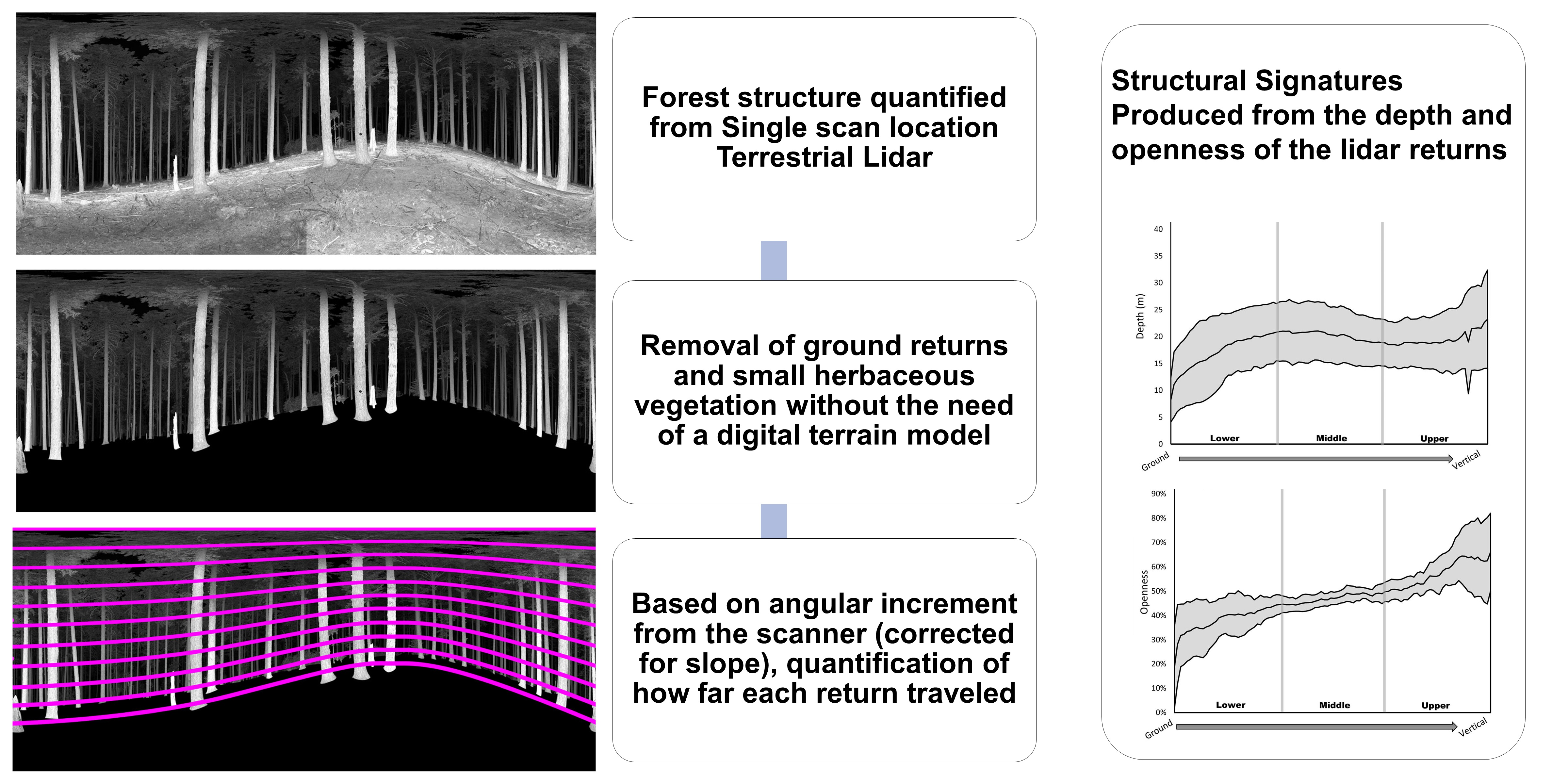
:We developed new measures of structural complexity using single point terrestrial laser scanning (TLS) point clouds. These metrics are depth, openness, and isovist. Depth is a three-dimensional, radial measure of the visible distance in all directions from plot center. Openness is the percent of scan pulses in the near-omnidirectional view without a return. Isovists are a measurement of the area visible from the scan location, a quantified measurement of the viewshed within the forest canopy. 243 scans were acquired in 27 forested stands in the Pacific Northwest region of the United States, in different ecoregions representing a broad gradient in structural complexity. All stands were designated natural areas with little to no human perturbations. We created “structural signatures” from depth and openness metrics that can be used to qualitatively visualize differences in forest structures and quantitively distinguish the structural composition of a forest at differing height strata. In most cases, the structural signatures of stands were effective at providing statistically significant metrics differentiating forests from various ecoregions and growth patterns. Isovists were less effective at differentiating between forested stands across multiple ecoregions, but they still quantify the ecological important metric of occlusion. These new metrics appear to capture the structural complexity of forests with a high level of precision and low observer bias and have great potential for quantifying structural change to forest ecosystems, quantifying effects of forest management activities, and describing habitat for organisms. Our measures of structure can be used to ground truth data obtained from aerial lidar to develop models estimating forest structure.
Keywords:
terrestrial lidar; TLS; forest structure; depth; openness; viewshed; Research Natural Areas; forest vegetation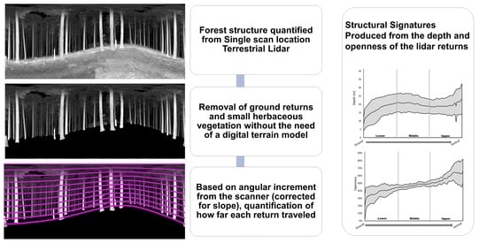
1. Introduction
1.1. Importance of Structure
The structural complexity of a forest (e.g., arrangement and amount of above-ground, biophysical components) has profound influences on its ecological function and health [1,2,3]. Structural complexity influences everything from canopy closure and connectivity that determines the amount of light infiltration to the forest floor, which influences the type and amount of understory and midstory plant species. Biophysical components also heavily influence the foraging and movement patterns of wildlife [4,5,6,7].
Quantifying structure is becoming increasingly important for resolving contemporary forest management issues. In the Pacific Northwest (PNW) of the United States, efforts to address some of these issues include developing late seral forest characteristics in young, managed forests to promote habitat for threatened northern spotted owls (Strix occidentalis caurina), landscape-level efforts to reduce fire fuel loads in dry forests after more than a century of fire suppression, and developing programs to monitor the long-term effects of climate change on natural and managed forests [8,9,10,11]. Each of these efforts requires, in part, the ability to quantify changes in the physical arrangement and amount of forest structure over time.
Historical measures of structural complexity have included simple measures of structural elements (e.g., tree diameter, height, spacing, basal area, variance in diameter at breast height (DBH)) and indices combining multiple measures (e.g., Shannon-Weiner Index, old growth index, & diameter diversity index [DDI]) [12,13,14,15]. These measures have been used successfully for a range of ecological applications, from single species habitat analysis at a localized level, to broad landscape-level planning [16,17]. Given the importance of forest structure, new methods are constantly being developed to quantify more nuanced and subtle differences and changes as new technologies emerge [18,19,20]. While most historical measures have relied on rudimentary hand tools, such as spherical densitometers or wedge prisms that introduce observer bias [21,22], many of the new methods to quantify forest structure leverage the more objective measurements derived from remote sensing platforms such as lidar.
1.2. Lidar for Forest Structure
Lidar technology is increasingly being used for quantifying forest structure [23,24,25]. Lidar data can be acquired from a variety of platforms, depending on the accuracy, resolution, and spatial coverage needed. Airborne lidar can efficiently capture forest structure across broad landscapes and has been used effectively to measure tree heights, leaf area index, above ground biomass, and forest heterogeneity [25,26,27,28]. Aerial lidar is so ingrained in current forest inventory assessments that it is a standard tool employed by many management organizations [29,30,31]. However, airborne lidar can miss much of the structural complexity in understory and midstory layers, particularly in dense forests; hence, efforts to quantify understory vegetation from ALS are limited in their characterizations [32,33,34].
Terrestrial laser scanning (TLS), also referred to as terrestrial lidar, is used to collect structural data from the ground and provides much more detailed information about the lower and middle layers of a forest than airborne lidar, especially in structurally complex forests where tree canopies can obscure aerial detection of understory and mid-story vegetation layers. Inversely, the upper canopy can be occluded from TLS in these same structurally complex and dense forests. The resolution of TLS is also much finer, with several hundred to many thousands of point returns captured per square meter (compared to a few dozen for airborne lidar). Although limited in area covered, TLS only requires a single operator and can be collected at any time weather conditions are favorable. TLS is increasingly being used to measure structural elements such as amount of woody biomass and basal area [35,36,37]. TLS has also been used to assess fire fuel loads and help predict fire behavior [38,39,40]. Further, TLS has been used to quantify forest structure for ecological analyses, including measuring forest stratification, wildlife habitat and prey cover, and structural density [41,42,43,44].
Typically, studies using TLS for forestry applications use multiple scans stitched together to create a comprehensive three-dimensional model. TLS point clouds are highly susceptible to occlusion as close objects block everything located behind them relative to the scanner position. The effects of this occlusion on derived forest metrics varies depending on what metrics are being obtained [45,46]. In relatively open forest stands, collecting multiple scans and creating a larger composite is a simple task of matching shared features between the scans (e.g., specific TLS targets or natural elements such as rocks or tree branches). In forest stands that have dense understory, stitching together multiple scans can be extremely difficult and time consuming due to the extreme amount of occlusion at each sampling location. Because of these limitations with using stitched together TLS scans, there is increasing interest in the use of single TLS scans to derive forest structural metrics. While single point TLS scans have been shown to be able to derive typical forest metrics such as DBH or stem maps [47,48,49], typically, multiple scans are required to replicate typical forest structure measurements [50]. The key to using single point TLS scans for forest structure characterization is likely to focus on deriving different types of metrics that still relate to forest structure beyond trying to replicate conventional sampling techniques (e.g., basal area and mean diameter). Richardson et al. [51] proposed the Three-dimensional Vegetation Density Index (3DI), which is a metric based on median distance traveled of each pulse between defined scan angles from the scanner. This method can quantify differences between stands with markedly different forest structure such as an area of dense understory vegetation compared to a stand where heavy cattle grazing removed much of the understory vegetation. However, there are some major limitations to the 3DI, namely that it does not account for slope effects on lidar point distances and thus can only be used effectively in relatively flat areas.
Studies that have used single TLS scans for novel ecological characterizations include using voxelization and point height statistics to quantify burn severity [52,53], using relative point location, geometry, and intensity to differentiate between tree stems and leaves [54], and correlating point height statistics with species richness [55]. While there has been work deriving forest metrics from single terrestrial lidar scans, only a small portion explicitly deal with how far individual pulses travel [56] or requires multiple scans to assess view area [57].
1.3. Objectives
We propose three different sets of metrics derived from single point TLS scans; depth, openness, and isovists. All three of these metrics are created in a manner that contours to localized plot topography and can be derived at sites that are both level and on a significant slope. Depth is a measurement of the distance traveled by each individual laser pulse stratified by the angle of the pulse leaving the scanner and corrected for slope. Openness accounts for pulses that did not return to the scanner (i.e., did not interact with any vegetation within the range of the scanner). Isovists, quantify the area visible approximately at 1.4 m above ground level with a 360° view from a center location. This metric is expressed as a percentage of total area visible at differing distances from the scanner. We generated our metrics from TLS scans collected in natural (no previous timber harvesting or other major human disturbance) forests that varied in structural complexity and composition to explore whether the expected variation in forest structure could be distinguished using our proposed metrics.
We then outline potential applications of these new metrics and discuss the potential advantages and disadvantages of using single TLS scans to quantify forest structure parameters.
2. Materials and Methods
2.1. Site Selection
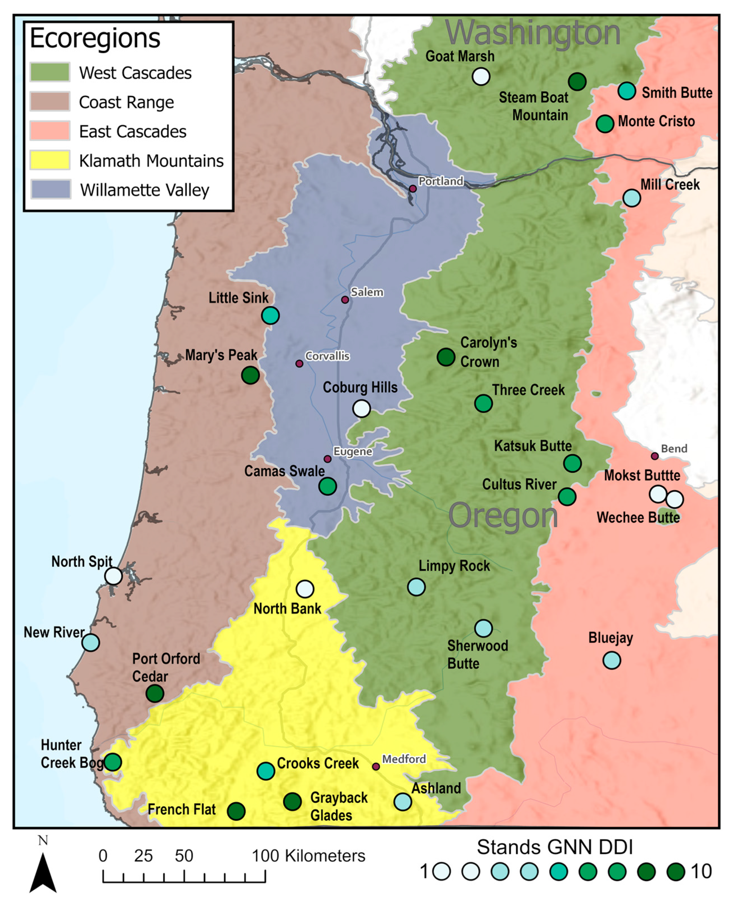
We selected twenty-seven forested stands across six ecoregions (Coast Range, Klamath Mountains, Willamette Valley, West Cascades, and East Cascades [58]) within a 300 km radius of Corvallis, Oregon for study. We chose stands within Forest Service and Bureau of Land Management, Research Natural Areas (RNAs) and Areas of Critical Environmental Concern (ACECs) because they represent relatively pristine forests with minimal anthropogenic influence and allowed us to explore a wide range of natural variation in forest structure [59] (Figure 1).
We used DDI as the primary metric for selecting stands that collectively represented a gradient in structural complexity across the study area. DDI is a measure based on counts of trees in four different size classes, with 0 indicating the absence of trees (non-forest) and 10 indicating maximum representation of 4 size classes [13]. DDI values were derived using gradient nearest neighbor (GNN) raster maps developed from LandSat satellite data [60]. Site selection was done remotely using ESRI GIS software [61] and relevant data layers. DDI raster values were smoothed using focal statistics, generating mean values within a 3 × 3 cell dimension neighborhood. We divided forested DDI values (i.e., values from 1–10) into nine classes (Table 1) and delineated patches of forest (i.e., stands) large enough to include 9 plots (3 × 3 grid, with 100 m spacing between grid points). From this pool of potential stands, we randomly selected three stands for each DDI class that could accommodate our plot grid to determine plot coordinates. We reselected a few stands due to access issues.
2.2. Scan Acquisition
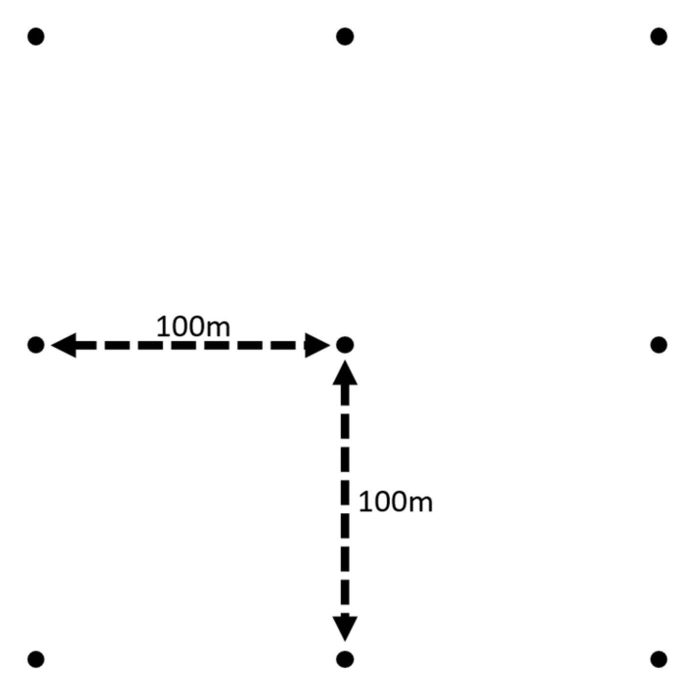
One scan was taken at each plot location for a total of 243 scans across the 27 stands (Figure 2). Scans were taken between 20 August and 9 October 2014, prior to leaf fall. A Faro Focus 3D s120 terrestrial lidar scanner (Faro Technologies Inc., Laker Mary, FL, USA) was used. Plot centers were located with a Garmin GPSmap handheld GPS unit (Garmin Ltd., Olathe, KS, USA) with 5 m to 20 m accuracy depending on canopy closure and weather conditions. TLS unit was set up at the plot center at approximately 1.4 m above ground. Some variation in scanner height was due to topography. If the plot center was too heavily occluded (e.g., within a dense shrub or directly next to a large tree) then the closest location to plot center that offered a full 360° of the stand within 10 m of plot center was used. This was to maximize area captured in the scan and to minimize occlusion by trees and shrubs. The scanner reliably received returns for objects ≤60 m away within a panoramic scan capturing a horizontal window from 0 to 360° and a vertical window from −60 to 90°. Vertical and horizontal scan lines were spaced every 0.035°, resulting in a 10,266 horizontal × 4267 vertical resolution per scan. Each scan required approximately 10 min to complete once onsite.
2.3. Scan Processing
Initial scan processing consisted of filtering artifacts and noise present in the scan data using preset filters in Faro Scene version 5.3.3 [62]. Dark scan points were isolated using an intensity (return signal strength) threshold of 200. Stray or isolated scan points were removed using a grid size of 3 px, distance threshold of 0.02 m, and allocation threshold of 33.3%. Noise and edge effects are inherent in all lidar data due to edge effects and back scattering [63].
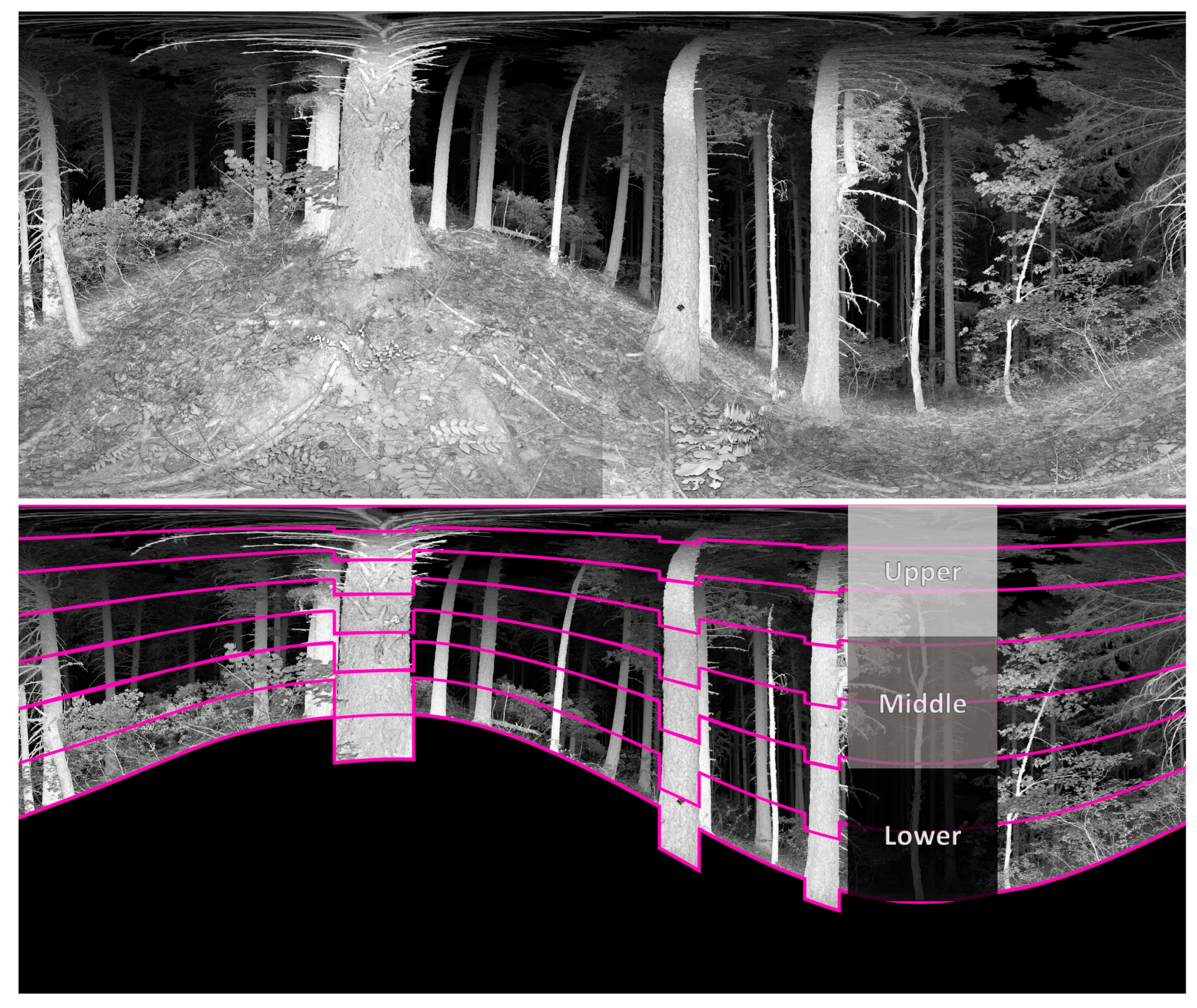
Processed scans were exported into Leica PTX format, which preserved scanning acquisition structure with fixed angular increments between scan pulses [64]. We used PTX reader [65] to create two-dimensional intensity (Online Supplement: Supplement A) and depth (range) raster images using first-return point values, where each column of pixels represented an individual scan line and each pixel represented an angular location where the laser pulse was fired. Each scan resulted in a 10,266 × 4267 pixel raster, matching the scanline resolution settings of the scanner. Because the rasters are 2D representations of a 3D point cloud, there are distortions in the image. This is essentially a cylindrical projection of the point cloud. As long as pixels within the image are only compared to other pixels in the same relative horizontal position, the distortion will be equivalent and allow for valid comparisons. In these planar projections, if a scan is taken on a steep slope, the ground will take on a wave-like appearance with the uphill slope appearing taller in the image and the downhill slope appearing lowering the image (Figure 3).
This process of using raster depth maps to account for slope has significant advantages over traditional lidar normalization processes for single TLS scans. Traditional lidar normalization uses detailed ground models to remove elevation from each points Z value leaving only the height above ground for each point. Using a single scan, only the ground relatively near the scanner is captured. Slope, density of vegetation and other factors can rapidly occlude the ground beyond a few meters. Normalization is dependent on having a robust ground model which cannot be generated beyond the area directly adjacent to the scanner. Digital terrain models (DTMs) from airborne lidar can be used to normalize TLS scans but this relies on there being ALS data available for all locations and accurately geolocated scans. For our methods we only used the data collected from the single scan and were not reliant on additional data.
Further, normalizing changes the viewshed from the scan location. Branches that were visible can become occluded if normalized, and gaps form where occluded areas before normalizing are moved.
2.4. Depth and Openness Metric Calculation
The ground, small herbaceous vegetation, and small woody debris was visually identified and removed in each depth raster. This was accomplished by manually tracing the intersection where the trees and larger vegetation met the ground in the image. Conceptually this is depicted in Figure 3. Bézier curves were used to fit the contours of the “wavey” hillslope when appropriate. The line created through this process was a hillslope horizon line that accounted for vegetation. The ground and small vegetation pixels were simply deleted, and a null value added to the raster. The number of pixels above ground in each vertical scan line in the depth raster was divided into 100 equally spaced vertical increments using a custom MATLAB [66] script (Figure 3).
This discretization process minimized potential slope effects within and across plots. It also ensured that the same relative location on the trees present at a plot were being captured within the same vertical layer. The lowest of the 100 sections uniformly sampled the base of the trees while the highest of the 100 sections uniformly sampled the upper canopy. We averaged both depth and percent of “no returns” (openness) for each increment across the entire 360° horizontal view. Structural signatures were comprised of the average value across all 9 scan plots at each of the 100 angular increments, at each stand. One standard deviation from the mean included as a shaded band that is an indicator of the forest structural heterogeneity. Additionally, overall means were calculated for the upper, middle, and lower forest layers for both the depth and openness plots as structural indices.
2.5. Isovists
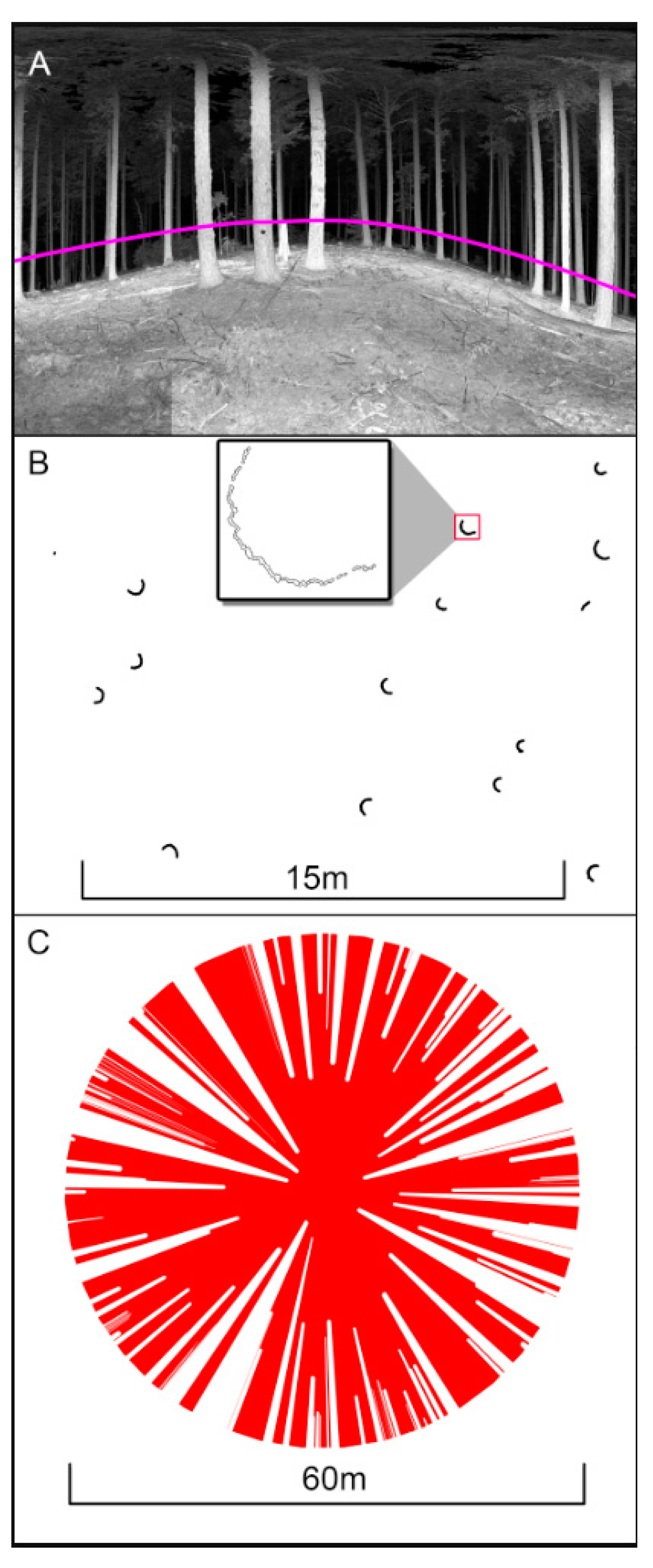
Isovists (polygons that enclose the visible area from a single vantage point) were generated for each plot. First, a polyline (4 pixels wide) was digitized on each intensity raster at 1.4 m above the ground (Figure 4A). Height above ground was determined by measuring a subset of trees (3–8, depending on slope) in the scan using FARO Scene. Bézier curves were fitted connecting the 1.4 m marks on the trees and contoured to the hill slope. The number of trees varied depending on the number of visible trees in the scan. For a tree to be used, the base needed to be visible. A cross section of points that fell along this line was extracted using PTX reader and subsequently flattened to the XY plane by ignoring Z (elevation) values.
Points within each cross section were imported into ESRI GIS software [61]. A circular buffer was drawn around each point to account for the inherent gaps between sample points. Given that the scanner operated on fixed angular increments rather than fixed sampling distances, we increased the buffer size for each point as range from scanner increased, using the following equation:
where:
D_Bi = R_i·tan∅ + ∈
DB = the diameter of the buffer (m) at point i,
R = the 3D Euclidean range from the scanner at the sample point i,
∅ = the angular sampling incremental (0.035° for this study), and
∈ = a small tolerance value to provide overlap to avoid small data gaps (0.003 m for this study).
The points in each scan were clipped to a horizontal radius of 55 m using circular buffers from each cross section (Figure 4B). Isovist polygons were created by extending 10,266 rays (at 0.035° increments to match scan line intervals) from the scanner location on the cross section and creating a point where each ray intersected a point buffer. The percentage of visible area was calculated at 5 m radius increments from the plot center resulting in 11 values per scan. Percentage was used rather than the actual area value to normalize the isovist metric across all radii.
2.6. Comparisons
2.6.1. Depth and Openness Statistical Tests
Univariate linear regression was used to test for correlation (significant at 95% confidence) between depth and openness (mean and variance between plots in each stand) to ensure these variables were independent.
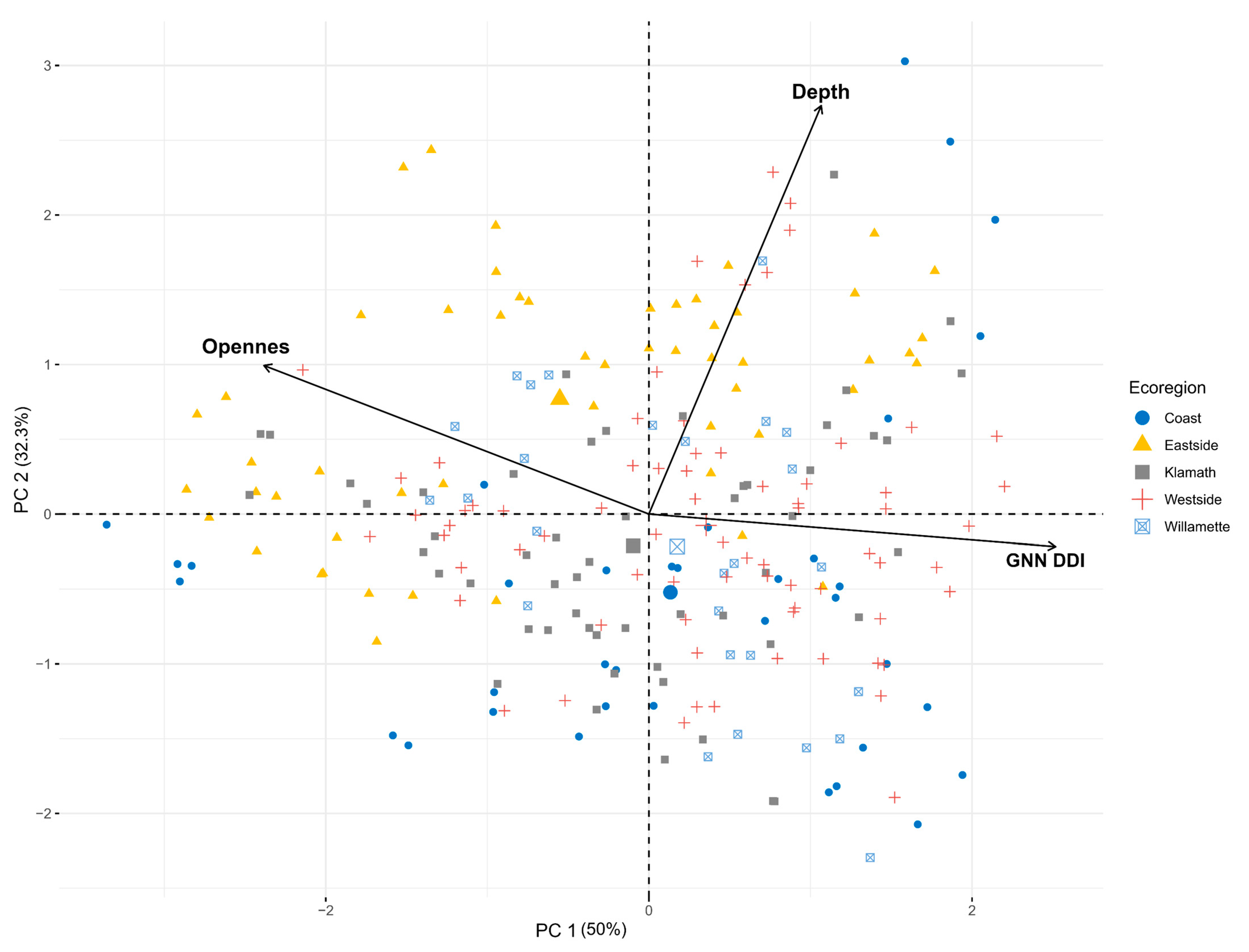
Principle componence analysis (PCA) [67] was used to visualize how well individual plots in each ecoregion clustered, to determine which depth and openness angular increments most contributed to PC 1 and PC 2, and to visualize the relationships between depth, openness, and GNN DDI vectors. Ordination was performed using all 243 plots with each plot having all depth and openness values assigned to it, resulting in a 243 × 200 main matrix and then simplified to only use the depth and openness angular increments that most contributed to PC 1 and PC 2, and the GNN DDI values. Data was scaled to unit variance before PCA was performed.
Analysis of variance (ANOVA) tests were used on depth and openness metrics at every angular increment with plots grouped by stands to determine if our new metrics differentiated between stands. For this step, 100 ANOVA tests were performed to test if there was a significant difference at each of the 100 angular increment sections between stands.
ANOVA tests using Tukey’s honestly significant difference (HSD) [68] was performed on plots using all 100 angular increment sections and grouping stands based on ecoregion to determine if our new metrics differentiated between forest structure based on ecoregion.
2.6.2. Isovist Statistical Tests
ANOVA tests were conducted for each isovist radius grouping isovists by stand. Stands were then aggregated into ecoregion groups to perform an ANOVA test with Tukey’s HSD post hoc intergroup comparisons.
3. Results
3.1. Structural Signatures
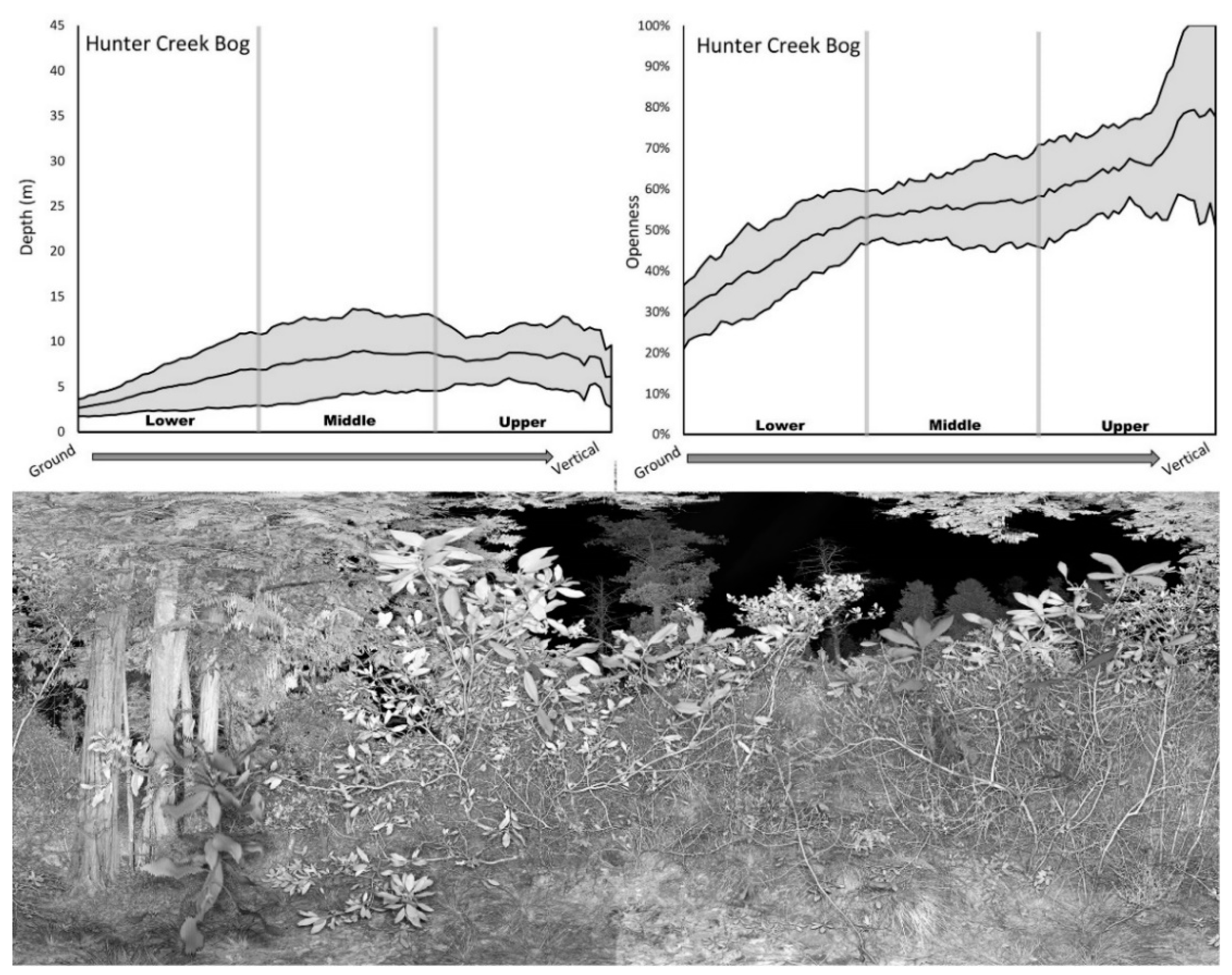
Each of the 27 stands exhibited distinctly different structural signatures for both depth and openness (Online Supplement: Supplement B). Some stands exhibited large amounts of structural variation at all vertical levels (e.g., Limpy Rock; Figure 5) while others exhibited relatively little variation (e.g., Hunter Creek Bog; Figure 5).
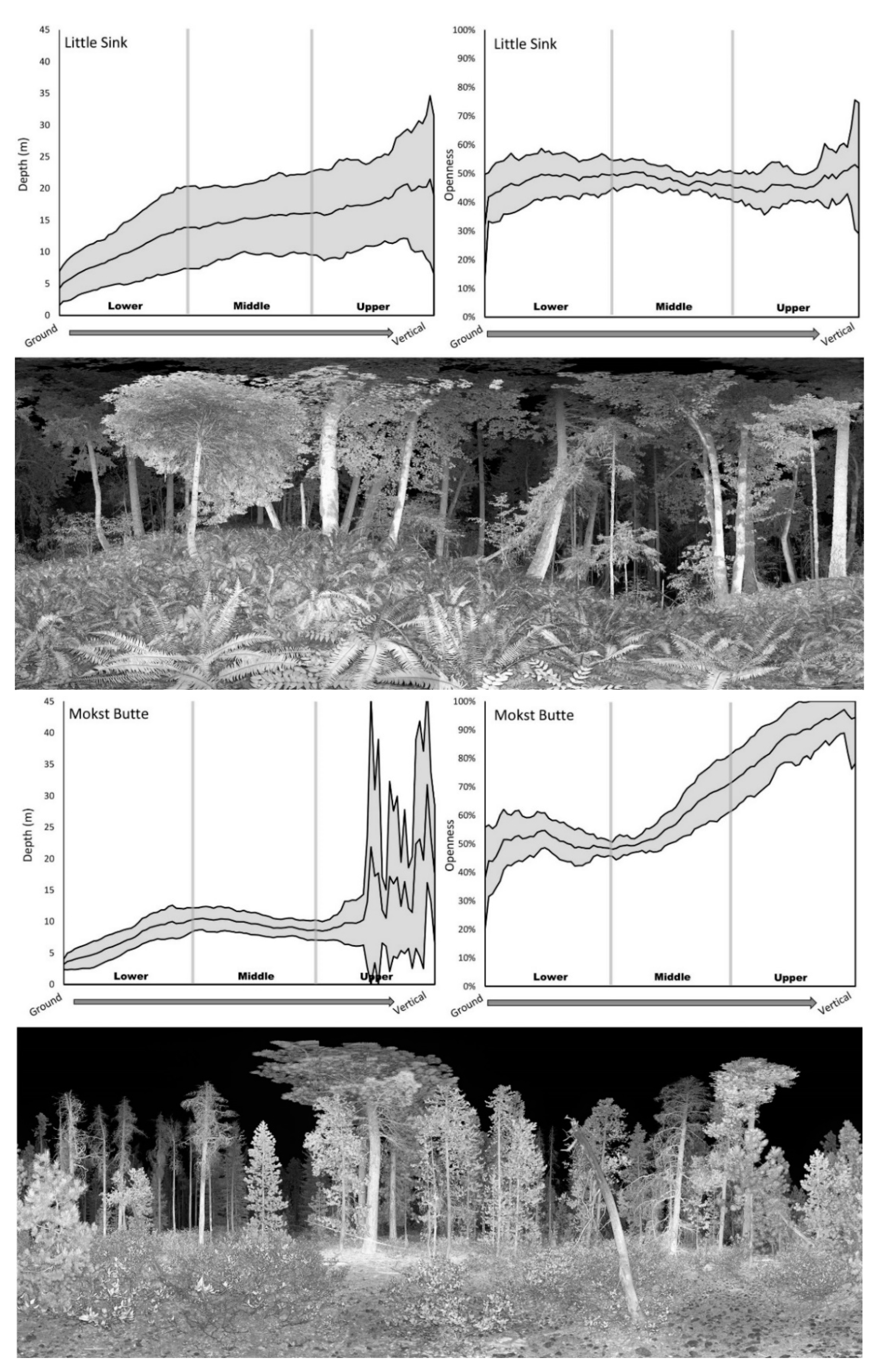
Some stands had increasing structural variation from the ground to the canopy (e.g., Little Sink; Figure 6). Other stands exhibited low variation in the lower and middle layers but abrupt increases in variation in the upper layers (e.g., Mokst Butte; Figure 6). Stands with dense understories tended to have low mean depth values (e.g., Hunter Creek Bog & Mokst Butte). Depth signature values tended to increase going from the ground to upper canopy. This increase was more rapid in stands with an open understory (e.g., Limpy Rock). Stands comprised of a mix of open and closed canopies could exhibit markedly varying depth signatures at the upper canopy layers (e.g., Mokst Butte). Stands with large canopy gaps had openness signatures that could reach 100% (e.g., Hunter Creek Bog and Mokst Butte). Stands with dense vegetation at all levels had a correspondingly low openness signature (e.g., Little Sink).
3.2. Depth and Openness Statistical Tests
No correlation was found between depth and openness (r2 < 0.01; p = 0.82) suggesting the two metrics were independent.
3.2.1. Ordination
The top 5 variables that most contributed to PC 1 were the depth angular increments 55 to 59. This is just above the middle view from the scanner (Figure 3). The top 5 variables that most contributed to PC 2 were the Openness angular increments 38 to 42. Our openness metric had a negative relationship to the GNN DDI values when only usingthe angular increments that most contributed to the PCA axis and adding the GNN DDI values (Figure 7).
3.2.2. Depth and Openness ANOVA
There were significant differences in the depth values between stands at each of the 100 angular increments (all p values < 0.05 with the majority < 2.2 × 10⁻¹⁶). There were also significant differences in the openness values between stands at each of the 100 angular increments (all p values < 0.05 with the majority < 2.2 × 10⁻¹⁶). With p values less than 0.05 for an ANOVA test, we accept the null hypothesis that at least one of the group means was significantly different than the others.
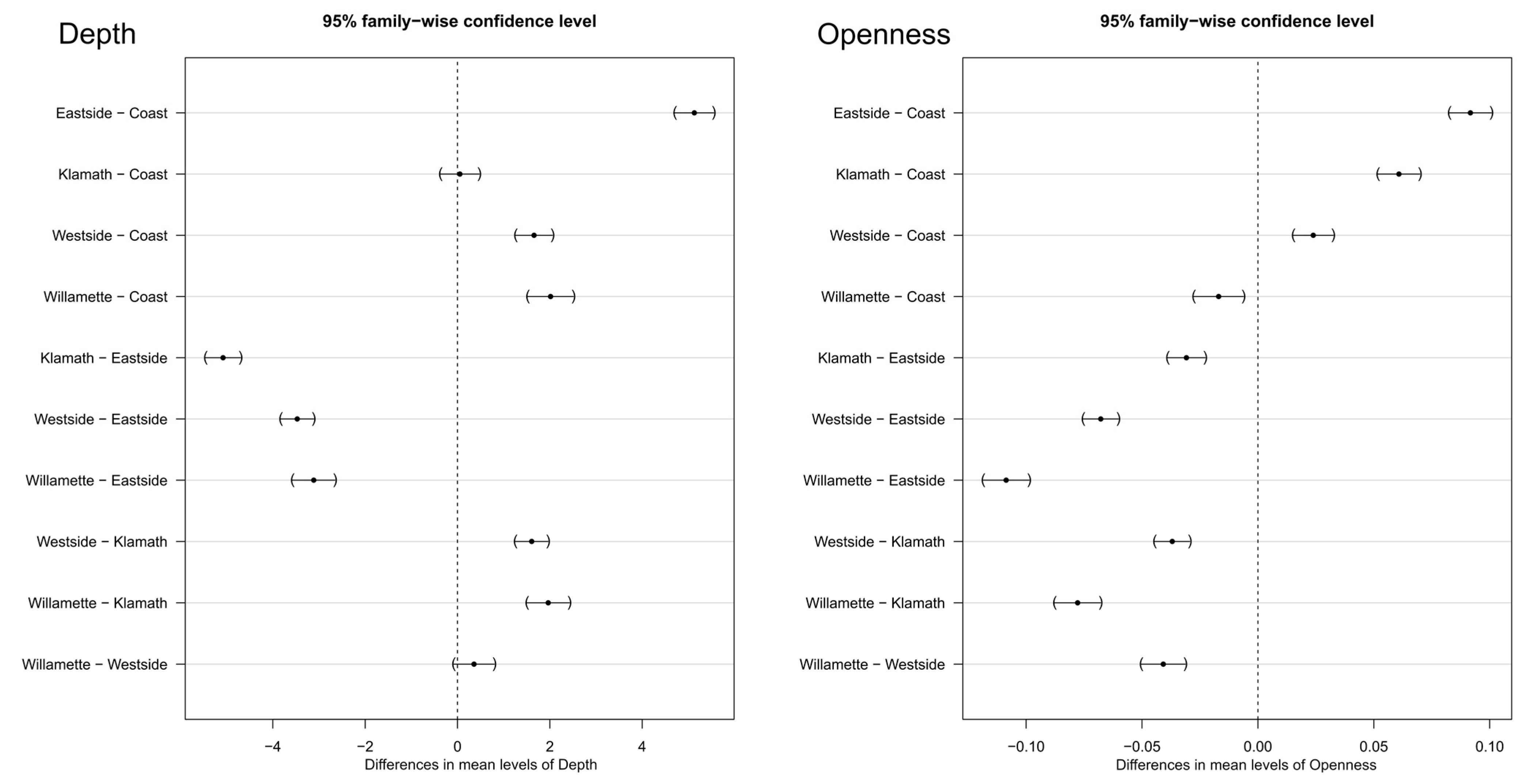
When grouped by ecoregion, there was a significant difference between all parings of the depth and openness metrics except for the depth metric between ecoregions of Klamath mountains and the coast range, as well as Willamette valley and the westside of the cascade mountains (Figure 8). Our stands in the eastside of the cascades were most dissimilar to stands in both the Klamath and coast ecoregions. Similar trends were also seen with the Openness metric.
3.3. Isovist Statistical Tests
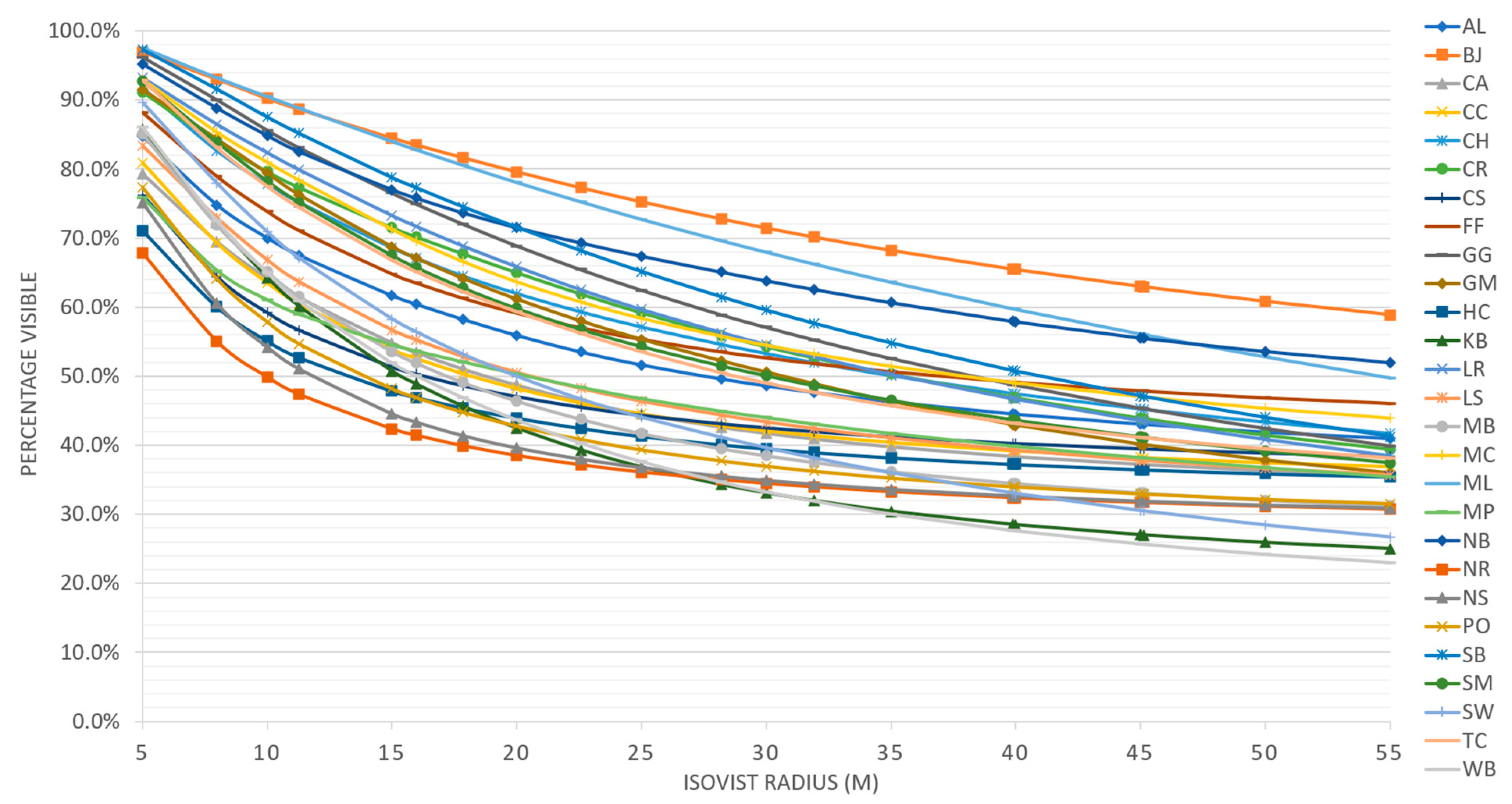
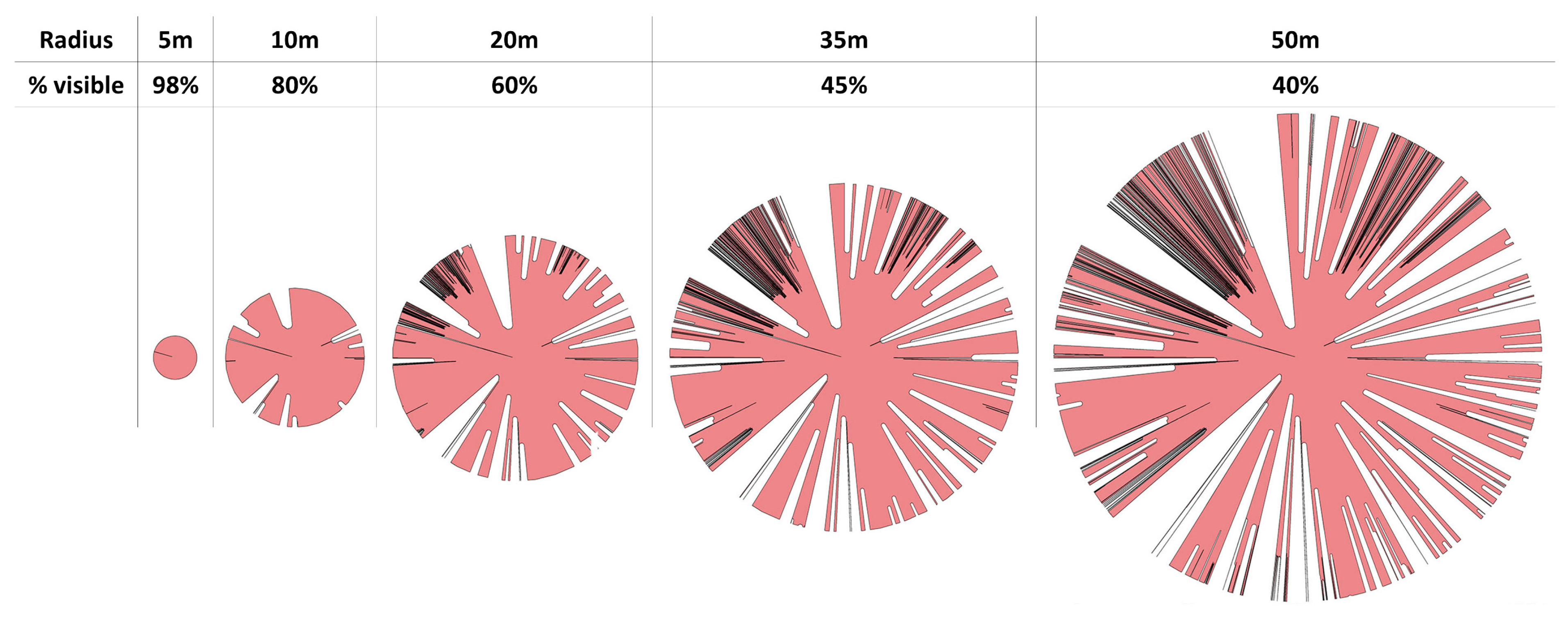
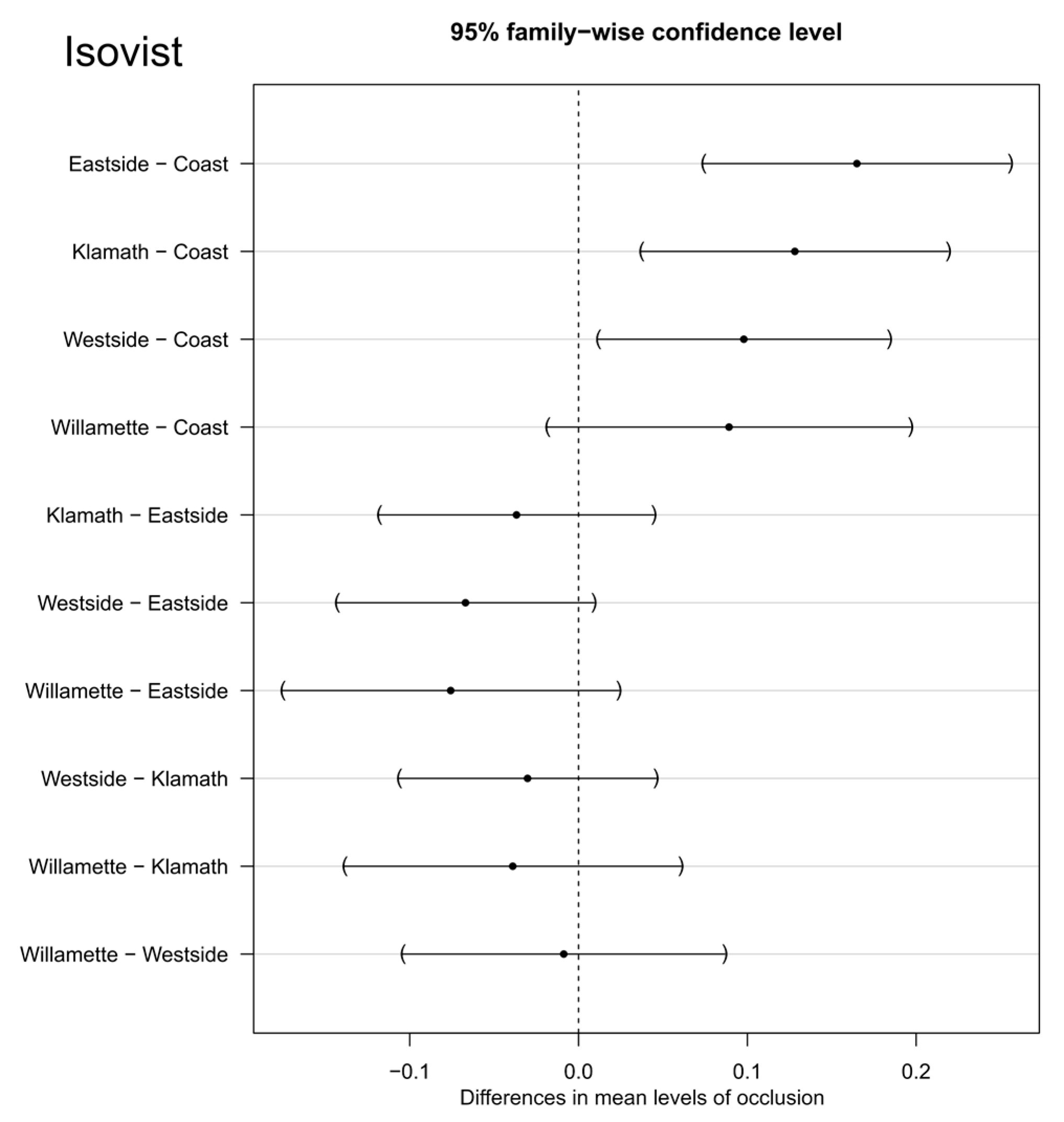
When grouped by stand, the isovist percentage of area visible was significantly different (p = 4.116 × 10⁻⁵). In general, the area visible decreased as the radius of the isovist increased (Figure 9 and Figure 10). This decrease was typically about 40%. The percentage visible ranking changed for many stands as the isovist polygon radius increased. For example, New River (NR) had the least area visible with a 5 m radius isovist but at 25 m and beyond, Wechee butte had the least area visible. While the rate of decrease was different between stands, the spread of percentage visible was about 30–35% for the 5 m distance all the way through the 55 m distance. When grouped by ecoregion, most of the combinations of ecoregions had no significant difference in averaged percentage visible. The only ecoregion that did have a statistically significant difference was the coast range (Figure 11).
4. Discussion
4.1. Depth and Openness
Our results suggest that depth and openness are two distinct measures of structural complexity. Each of our 27 stands exhibited unique signatures and could be clearly distinguished from each other, suggesting that both depth and openness can capture the unique variation in structural complexity found in natural forests and at relatively fine scales. The structural signatures can be qualitatively assessed for stand openness and heterogeneity while also providing quantitative values for statistical analysis.
One strength of these metrics is that specific height strata within a forest can be extracted. For example, if only understory vegetation is of interest, then only the lowest angular increment layers can be included in an analysis. Our suggestion of 100 angular increments is a subjectively assigned value and fewer, or more increments can be used as is warranted by the research question being addressed. It is important to consider that our sampling was not a horizontal metric of canopy slices at different height strata, but rather the angular view of different height strata from a ground perspective.
We have shown that the depth and openness metrics do return significantly different values for stands at every angular increment, but more importantly, they also can be used to differentiate forest structure when aggregated to ecoregion. The Tukey HSD results show which regions have dramatically different vegetation structures and which ecoregions tend to have structurally similar forests. Although not explicitly examined here, we would expect a much higher degree of similarity among signatures in young forests managed for timber production where within-stand structure tends to be relatively homogeneous (e.g., single tree species of a similar age cohort, uniform spacing between individual trees).
4.2. Isovists
The ability to quantify the structural differences between forest types and forest of different ecoregions was less using the isovist approach compared to our depth and openness metrics. However, this does not indicate that the isovists do not quantify an important element of forest structure, as they are a direct measure of visual occlusion. As such, their utility may be better suited to ecological questions where occlusion can be an important component of habitat. Many wildlife species change behavior based on the area visible at any given location or have active preferences for certain amounts of visibility for hunting, denning, or relaxation [43,69,70]. For example, Canada lynx (Lynx canadensis), a species of special conservation concern, appears to require high amounts of understory cover (i.e., lower percentage of area visible) as part of quality habitat [71,72].
Our metrics are a direct measurement of understory vegetation structure and occlusion that can be used as localized assessment of habitat quality. Beyond a localized assessment, these metrics offer a high potential to be used as ground truth data for upscaling on the ground measurements of understory vegetation structure to a region wide model using airborne lidar. Such upscaling and modeling has already been done using cover boards to quantify horizontal visibility levels [73], but we believe that TLS offers advantages over the more subjective coverboard estimates in both time and effort required to obtain the data as well as providing a more robust measurement of cover.
Calculating visual occlusion using TLS point clouds is not new. With robust multi-scan TLS point clouds 3D viewshed analysis has been done for several wildlife studies [74,75] using R packages such as viewshed3D [76]. The advantage of our method is the ability to correct for slope without a ground model, but undoubtedly if full and comprehensive multi-scan TLS point clouds are available then the generation of a 3D viewshed has obvious benefits over our 2D option.
4.3. Potential Applications
We suggest our new metrics have a wide range of potential applications for both management and research. For example, a primary goal for much of the timber harvesting on federal lands in the Pacific Northwest is to move the structural trajectories of young, managed forests towards characteristics more typical of late-seral forest. TLS signatures could be used to help define and describe the structural variation found in natural (un-managed) forests, including diverse late-seral forests as evaluated in this study. In managed forests, TLS signatures could help (1) assess pre-thinning structural condition; (2) assess immediate post-harvest condition to determine if thinning met structural goals; (3) monitor treated stands at regular intervals to follow the trajectory of structural development; and (4) establish benchmark data from relevant natural stands for desired future condition.
Biomass estimates may also be possible with our proposed metrics. Biomass is an important measurement as it relates to carbon storage, timber volume, and species habitat. If the foliage density and viewshed at different angular increments can be related to on the ground manual measurements of forest biomass, then such biomass measurements could be done at further areas with a greatly reduced labor cost. Multi position TLS sans are already widely used for biomass estimates [77,78,79] and biomass modeling from airborne and space borne lidar has provided valuable estimates [80,81,82], but there is still an excellent opportunity for future research deriving biomass estimates in highly occluded areas with a single point TLS scan.
A subset of the full signature may also help assess change and characteristics at different vertical strata within a forest. For example, upper canopy measures could be used to evaluate effects of defoliating pathogens and insects. Lower sections could be used to derive indices for understory shrub and sapling density or fire fuel loads. Similar to biomass estimates, TLS has seen considerable research to quantify fire fuel loads, but the vast majority of the work is dependent on multiple scans [38,39]. Both the point cloud data and photographs generated with each TLS scan could also be used to determine actual height layers of vegetation, and in some cases, plant species composition.
The point cloud data could be synthesized in other ways than we described here. For example, we chose to divide the vertical scan lines into 100 sections to create signatures because increasing the number of sections did not produce a visually discernible difference in the level of detail. The number of sections could be increased if a higher resolution signature was desired when more detail was necessary. There is also potential for further development of structural measures using three-dimensional isovists for measuring openness as distance increased in any direction.
4.4. Limitations
One important limitation of TLS is that the ability to detect objects diminishes with increasing distance to objects (reliability of scan returns diminished substantially > 60 m for this study). Multiple scans could be registered together to produce a more complete three-dimensional model of each plot. Not only would this allow three-dimensional modeling of individual trees, it would also allow calculation of structural signatures based on height above ground (rather than angular increment). However, labor costs (field and post-processing) to create these composite datasets would be markedly higher compared to single-point scans, especially for forests with high levels of occlusion. Additionally, initial filtering of the point clouds could have a substantial effect on our metrics. Structurally complex objects such as trees are especially susceptible to noise due to edge effects and backscattering. Overly aggressive point filtering can remove valid points and reduce point cloud accuracy [83]. We suspect our methods are likely very susceptible to errors due to noise and filtering and this is one avenue of future research. Lastly, while lidar technologies are becoming more common and ubiquitous within the field of forest ecology, the units are still expensive and the skillset to process data to final and meaningful ecological metrics requires extensive training.
For our processing we relied on manual removal of ground points within the raster depth maps and the creation of a hillslope horizon line that accounted for vegetation. This is a subjective process and needs refinement. For the purposes of accounting for slope, this process does have advantages over traditional lidar normalization for single scans, but further removing the subjective element would be ideal. There may be a way to create a hybrid approach by classifying ground points before creating raster depth maps and then removing all pixels within a set radius from a ground point. Further, this approach for accounting for slope does not account for micro topography and abrupt changes in slope.
5. Conclusions
While no single metric of structure can possibly satisfy all needs for all applications, we believe our depth and openness measures have significant advantages over many past measures for quantifying forest structure. In addition to capturing the multi-dimensional properties of forest structure, these new measures (1) are spatially and temporally scalable (a few centimeters to tens of meters) in all directions; (2) are precise with low observer bias; (3) can be rapidly collected in the field; (4) are based on point cloud data that is unlikely to become obsolete in the foreseeable future; and (5) can be further synthesized in ways to meet specific research questions and management needs. Next steps include testing the usefulness of these new measures for quantifying wildlife habitat and periodic (5 to10-yr) re-measurement of our study plots to test their sensitivity to capture structural change over time. Additionally, using these metrics as ground truth data to create regional models needs to be more fully explored. TLS metrics that are derived directly from point clouds may be better suited as model inputs to estimate forest structure using larger area data sets such as aerial lidar.
Supplementary Materials
The following are available online at https://0-www-mdpi-com.brum.beds.ac.uk/article/10.3390/rs15010145/s1, Supplement A—Lidar plot scan images; Supplement B—Lidar plot Signatures.
Author Contributions
Conceptualization, J.L.B., T.M.W., M.J.O., W.J.R.; methodology, J.L.B., T.M.W., M.J.O.; software, J.L.B., M.J.O.; formal analysis, J.L.B., T.M.W., M.J.O.; resources, T.M.W., W.J.R.; writing—original draft preparation, J.L.B.; writing—review and editing, T.M.W., M.J.O., W.J.R.; visualization, J.L.B.; supervision, T.M.W., M.J.O., W.J.R.; project administration, T.M.W.; funding acquisition, T.M.W., W.J.R. All authors have read and agreed to the published version of the manuscript.
Funding
Funding was provided by the USDI Bureau of Land Management, Oregon State Office, and the USDA Forest Service, Pacific Northwest Research Station.
Data Availability Statement
The data presented in this study are available on request from the corresponding author.
Acknowledgments
Luke Painter provided guidance and mentorship on manuscript preparation. We thank Leica Geosystems for providing Cyclone licenses used for exploratory analysis.
Conflicts of Interest
Michael Olsen has financial interests in the company EzDataMD LLC related to the commercialization of technology Involving point cloud analysis. The conduct, outcomes, or reporting of this research could benefit EzDataMD LLC and could potentially benefit them.
References
- Lindenmayer, D.B.; Franklin, J.F. Conserving Forest Biodiversity: A Comprehensive Multiscaled Approach; Island Press: Washington, DC, USA, 2002. [Google Scholar]
- Carey, A.B. AIMing for Healthy Forests: Active, Intentional Management for Multiple Values; General Technical Report PNW-GTR-721; U.S. Department of Agriculture, Forest Service, Pacific Northwest Research Station: Portland, OR, USA, 2007.
- Shugart, H.; Saatchi, S.; Hall, F. Importance of Structure and Its Measurement in Quantifying Function of Forest Ecosystems. J. Geophys. Res. Biogeosci. 2010, 115. [Google Scholar] [CrossRef]
- Chazdon, R.L. Sunflecks and Their Importance to Forest Understorey Plants. Adv. Ecol. Res. 1988, 18, 1–63. [Google Scholar]
- Beier, P.; Drennan, J.E. Forest Structure and Prey Abundance in Foraging Areas of Northern Goshawks. Ecol. Appl. 1997, 7, 564–571. [Google Scholar] [CrossRef]
- Pardini, R.; de Souza, S.M.; Braga-Neto, R.; Metzger, J.P. The Role of Forest Structure, Fragment Size and Corridors in Maintaining Small Mammal Abundance and Diversity in an Atlantic Forest Landscape. Biol. Conserv. 2005, 124, 253–266. [Google Scholar] [CrossRef]
- Musselman, K.N.; Molotch, N.P.; Margulis, S.A.; Kirchner, P.B.; Bales, R.C. Influence of Canopy Structure and Direct Beam Solar Irradiance on Snowmelt Rates in a Mixed Conifer Forest. Agric. For. Meteorol. 2012, 161, 46–56. [Google Scholar] [CrossRef]
- Davis, C.R.; Belote, T.; Williamson, M.; Larson, A.; Esch, B. A Rapid Forest Assessment Method for Multiparty Monitoring across Landscapes. J. For. 2016, 114, 125–133. [Google Scholar] [CrossRef]
- Everett, R.L.; Leader, A.T. Eastside Forest Ecosystem Health Assessment; General Technical Report PNW-GTR-330; U.S. Department of Agriculture, Forest Service, Pacific Northwest Research Station: Portland, OR, USA, 1994.
- Massie, M. Assessment of the Vulnerability of Oregon and Washington’s Natural Areas to Climate Change. Master’s Thesis, Oregon State University, Portland, OR, USA, 2014. [Google Scholar]
- Rapp, V. Northwest Forest Plan—The First 10 Years (1994–2003): First-Decade Results of the Northwest Forest Plan; General Technical Report PNW-GTR-720; U.S. Department of Agriculture, Forest Service, Pacific Northwest Research Station: Portland, OR, USA, 2008.
- Acker, S.A.; Sabin, T.E.; Ganio, L.M.; McKee, W.A. Development of Old-Growth Structure and Timber Volume Growth Trends in Maturing Douglas-Fir Stands. For. Ecol. Manag. 1998, 104, 265–280. [Google Scholar] [CrossRef]
- McComb, W.C.; McGrath, M.T.; Spies, T.A.; Vesely, D. Models for Mapping Potential Habitat at Landscape Scales: An Example Using Northern Spotted Owls. For. Sci. 2002, 48, 203–216. [Google Scholar]
- McElhinny, C.; Gibbons, P.; Brack, C.; Bauhus, J. Forest and Woodland Stand Structural Complexity: Its Definition and Measurement. For. Ecol. Manag. 2005, 218, 1–24. [Google Scholar] [CrossRef]
- Staudhammer, C.L.; LeMay, V.M. Introduction and Evaluation of Possible Indices of Stand Structural Diversity. Can. J. For. Res. 2001, 31, 1105–1115. [Google Scholar] [CrossRef]
- Tuchmann, E.T.; Connaughton, K.P. The Northwest Forest Plan: A Report to the President and Congress; DIANE Publishing: Collingdale, PA, USA, 1998. [Google Scholar]
- Pommerening, A. Approaches to Quantifying Forest Structures. Forestry 2002, 75, 305–324. [Google Scholar] [CrossRef]
- Bruggisser, M.; Hollaus, M.; Kükenbrink, D.; Pfeifer, N. Comparison of Forest Structure Metrics Derived from UAV Lidar and ALS Data. ISPRS Ann. Photogramm. Remote Sens. Spat. Inf. Sci. 2019, 4, 325–332. [Google Scholar] [CrossRef]
- Moeser, D.; Morsdorf, F.; Jonas, T. Novel Forest Structure Metrics from Airborne LiDAR Data for Improved Snow Interception Estimation. Agric. For. Meteorol. 2015, 208, 40–49. [Google Scholar] [CrossRef]
- Uuemaa, E.; Antrop, M.; Roosaare, J.; Marja, R.; Mander, Ü. Landscape Metrics and Indices: An Overview of Their Use in Landscape Research. Living Rev. Landsc. Res. 2009, 3, 1–28. [Google Scholar] [CrossRef]
- Frey, J.; Joa, B.; Schraml, U.; Koch, B. Same Viewpoint Different Perspectives—A Comparison of Expert Ratings with a TLS Derived Forest Stand Structural Complexity Index. Remote Sens. 2019, 11, 1137. [Google Scholar] [CrossRef] [Green Version]
- Vales, D.J.; Bunnell, F.L. Comparison of Methods for Estimating Forest Overstory Cover. I. Observer Effects. Can. J. For. Res. 1988, 18, 606–609. [Google Scholar]
- Beland, M.; Parker, G.; Sparrow, B.; Harding, D.; Chasmer, L.; Phinn, S.; Antonarakis, A.; Strahler, A. On Promoting the Use of Lidar Systems in Forest Ecosystem Research. For. Ecol. Manag. 2019, 450, 117484. [Google Scholar] [CrossRef]
- Camarretta, N.; Harrison, P.A.; Bailey, T.; Potts, B.; Lucieer, A.; Davidson, N.; Hunt, M. Monitoring Forest Structure to Guide Adaptive Management of Forest Restoration: A Review of Remote Sensing Approaches. New For. 2020, 51, 573–596. [Google Scholar] [CrossRef]
- Wulder, M.A.; White, J.C.; Nelson, R.F.; Næsset, E.; Ørka, H.O.; Coops, N.C.; Hilker, T.; Bater, C.W.; Gobakken, T. Lidar Sampling for Large-Area Forest Characterization: A Review. Remote Sens. Environ. 2012, 121, 196–209. [Google Scholar] [CrossRef] [Green Version]
- Calders, K.; Lewis, P.; Disney, M.; Verbesselt, J.; Herold, M. Investigating Assumptions of Crown Archetypes for Modelling LiDAR Returns. Remote Sens. Environ. 2013, 134, 39–49. [Google Scholar] [CrossRef]
- Zimble, D.A.; Evans, D.L.; Carlson, G.C.; Parker, R.C.; Grado, S.C.; Gerard, P.D. Characterizing Vertical Forest Structure Using Small-Footprint Airborne LiDAR. Remote Sens. Environ. 2003, 87, 171–182. [Google Scholar] [CrossRef] [Green Version]
- Ackers, S.H.; Davis, R.J.; Olsen, K.A.; Dugger, K.M. The Evolution of Mapping Habitat for Northern Spotted Owls (Strix Occidentalis Caurina): A Comparison of Photo-Interpreted, Landsat-Based, and Lidar-Based Habitat Maps. Remote Sens. Environ. 2015, 156, 361–373. [Google Scholar] [CrossRef]
- Coops, N.C.; Tompalski, P.; Goodbody, T.R.; Queinnec, M.; Luther, J.E.; Bolton, D.K.; White, J.C.; Wulder, M.A.; van Lier, O.R.; Hermosilla, T. Modelling Lidar-Derived Estimates of Forest Attributes over Space and Time: A Review of Approaches and Future Trends. Remote Sens. Environ. 2021, 260, 112477. [Google Scholar] [CrossRef]
- Lister, A.J.; Andersen, H.; Frescino, T.; Gatziolis, D.; Healey, S.; Heath, L.S.; Liknes, G.C.; McRoberts, R.; Moisen, G.G.; Nelson, M. Use of Remote Sensing Data to Improve the Efficiency of National Forest Inventories: A Case Study from the United States National Forest Inventory. Forests 2020, 11, 1364. [Google Scholar] [CrossRef]
- Tinkham, W.T.; Mahoney, P.R.; Hudak, A.T.; Domke, G.M.; Falkowski, M.J.; Woodall, C.W.; Smith, A.M. Applications of the United States Forest Inventory and Analysis Dataset: A Review and Future Directions. Can. J. For. Res. 2018, 48, 1251–1268. [Google Scholar] [CrossRef]
- Campbell, M.J.; Dennison, P.E.; Hudak, A.T.; Parham, L.M.; Butler, B.W. Quantifying Understory Vegetation Density Using Small-Footprint Airborne Lidar. Remote Sens. Environ. 2018, 215, 330–342. [Google Scholar] [CrossRef]
- Hilker, T.; van Leeuwen, M.; Coops, N.C.; Wulder, M.A.; Newnham, G.J.; Jupp, D.L.B.; Culvenor, D.S. Comparing Canopy Metrics Derived from Terrestrial and Airborne Laser Scanning in a Douglas-Fir Dominated Forest Stand. Trees 2010, 24, 819–832. [Google Scholar] [CrossRef]
- Ruiz, L.Á.; Crespo-Peremarch, P.; Torralba, J. Modelling Canopy Fuel Properties and Understory Vegetation with Full-Waveform LiDAR. In Proceedings of the International Conference on Smart Geoinformatics Applications (ICSGA 2021), Phuket, Thailand, 24–25 February 2021; pp. 29–32. [Google Scholar]
- Calders, K.; Adams, J.; Armston, J.; Bartholomeus, H.; Bauwens, S.; Bentley, L.P.; Chave, J.; Danson, F.M.; Demol, M.; Disney, M.; et al. Terrestrial Laser Scanning in Forest Ecology: Expanding the Horizon. Remote Sens. Environ. 2020, 251, 112102. [Google Scholar] [CrossRef]
- Henning, J.G.; Radtke, P.J. Detailed Stem Measurements of Standing Trees from Ground-Based Scanning Lidar. For. Sci. 2006, 52, 67–80. [Google Scholar]
- Palace, M.; Sullivan, F.B.; Ducey, M.; Herrick, C. Estimating Tropical Forest Structure Using a Terrestrial Lidar. PLoS ONE 2016, 11, e0154115. [Google Scholar] [CrossRef] [Green Version]
- Loudermilk, E.L.; Hiers, J.K.; O’Brien, J.J.; Mitchell, R.J.; Singhania, A.; Fernandez, J.C.; Cropper, W.P.; Slatton, K.C. Ground-Based LIDAR: A Novel Approach to Quantify Fine-Scale Fuelbed Characteristics. Int. J. Wildland Fire 2009, 18, 676–685. [Google Scholar] [CrossRef] [Green Version]
- Rowell, E.; Loudermilk, E.L.; Hawley, C.; Pokswinski, S.; Seielstad, C.; Queen, L.; O’Brien, J.J.; Hudak, A.T.; Goodrick, S.; Hiers, J.K. Coupling Terrestrial Laser Scanning with 3D Fuel Biomass Sampling for Advancing Wildland Fuels Characterization. For. Ecol. Manag. 2020, 462, 117945. [Google Scholar] [CrossRef]
- Wilson, N.; Bradstock, R.; Bedward, M. Detecting the Effects of Logging and Wildfire on Forest Fuel Structure Using Terrestrial Laser Scanning (TLS). For. Ecol. Manag. 2021, 488, 119037. [Google Scholar] [CrossRef]
- Ashcroft, M.B.; Gollan, J.R.; Ramp, D. Creating Vegetation Density Profiles for a Diverse Range of Ecological Habitats Using Terrestrial Laser Scanning. Methods Ecol. Evol. 2014, 5, 263–272. [Google Scholar] [CrossRef]
- Kazakova, A.N. Quantifying Vertical and Horizontal Stand Structure Using Terrestrial LiDAR in Pacific Northwest Forests. Master’s Thesis, University of Washington, Seattle, WA, USA, 2014. [Google Scholar]
- Olsoy, P.J.; Forbey, J.S.; Rachlow, J.L.; Nobler, J.D.; Glenn, N.F.; Shipley, L.A. Fearscapes: Mapping Functional Properties of Cover for Prey with Terrestrial LiDAR. BioScience 2015, 65, 74–80. [Google Scholar] [CrossRef] [Green Version]
- Shokirov, S.; Levick, S.R.; Jucker, T.; Yeoh, P.; Youngentob, K. Comparison of TLS and ULS Data for Wildlife Habitat Assessments in Temperate Woodlands. In Proceedings of the IGARSS 2020—2020 IEEE International Geoscience and Remote Sensing Symposium, Online, 26 September–2 October 2020; pp. 6097–6100. [Google Scholar]
- Soma, M.; Pimont, F.; Allard, D.; Fournier, R.; Dupuy, J.-L. Mitigating Occlusion Effects in Leaf Area Density Estimates from Terrestrial LiDAR through a Specific Kriging Method. Remote Sens. Environ. 2020, 245, 111836. [Google Scholar] [CrossRef]
- Wan, P.; Wang, T.; Zhang, W.; Liang, X.; Skidmore, A.K.; Yan, G. Quantification of Occlusions Influencing the Tree Stem Curve Retrieving from Single-Scan Terrestrial Laser Scanning Data. For. Ecosyst. 2019, 6, 43. [Google Scholar] [CrossRef] [Green Version]
- Litkey, P.; Liang, X.; Kaartinen, H.; Hyyppä, J.; Kukko, A.; Holopainen, M.; Hill, R.; Rosette, J.; Suárez, J. Single-Scan TLS Methods for Forest Parameter Retrieval. In Proceedings of the SilviLaser, Edinburgh, UK, 17–19 September 2008. [Google Scholar]
- Xia, S.; Wang, C.; Pan, F.; Xi, X.; Zeng, H.; Liu, H. Detecting Stems in Dense and Homogeneous Forest Using Single-Scan TLS. Forests 2015, 6, 3923–3945. [Google Scholar] [CrossRef] [Green Version]
- Pokswinski, S.; Gallagher, M.R.; Skowronski, N.S.; Loudermilk, E.L.; Hawley, C.; Wallace, D.; Everland, A.; Wallace, J.; Hiers, J.K. A Simplified and Affordable Approach to Forest Monitoring Using Single Terrestrial Laser Scans and Transect Sampling. MethodsX 2021, 8, 101484. [Google Scholar] [CrossRef]
- Moskal, L.M.; Zheng, G. Retrieving Forest Inventory Variables with Terrestrial Laser Scanning (TLS) in Urban Heterogeneous Forest. Remote Sens. 2011, 4, 1–20. [Google Scholar] [CrossRef] [Green Version]
- Richardson, J.J.; Moskal, L.M.; Bakker, J.D. Terrestrial Laser Scanning for Vegetation Sampling. Sensors 2014, 14, 20304–20319. [Google Scholar] [CrossRef] [PubMed] [Green Version]
- Kato, A.; Moskal, L.M.; Batchelor, J.L.; Thau, D.; Hudak, A.T. Relationships between Satellite-Based Spectral Burned Ratios and Terrestrial Laser Scanning. Forests 2019, 10, 444. [Google Scholar] [CrossRef] [Green Version]
- Gallagher, M.R.; Maxwell, A.E.; Guillén, L.A.; Everland, A.; Loudermilk, E.L.; Skowronski, N.S. Estimation of Plot-Level Burn Severity Using Terrestrial Laser Scanning. Remote Sens. 2021, 13, 4168. [Google Scholar] [CrossRef]
- Tan, K.; Ke, T.; Tao, P.; Liu, K.; Duan, Y.; Zhang, W.; Wu, S. Discriminating Forest Leaf and Wood Components in TLS Point Clouds at Single-Scan Level Using Derived Geometric Quantities. IEEE Trans. Geosci. Remote Sens. 2021, 60, 1–17. [Google Scholar] [CrossRef]
- Anderson, C.T.; Dietz, S.L.; Pokswinski, S.M.; Jenkins, A.M.; Kaeser, M.J.; Hiers, J.K.; Pelc, B.D. Traditional Field Metrics and Terrestrial LiDAR Predict Plant Richness in Southern Pine Forests. For. Ecol. Manag. 2021, 491, 119118. [Google Scholar] [CrossRef]
- Wallace, L.; Hillman, S.; Hally, B.; Taneja, R.; White, A.; McGlade, J. Terrestrial Laser Scanning: An Operational Tool for Fuel Hazard Mapping? Fire 2022, 5, 85. [Google Scholar] [CrossRef]
- Murgoitio, J.; Shrestha, R.; Glenn, N.; Spaete, L. Airborne LiDAR and Terrestrial Laser Scanning Derived Vegetation Obstruction Factors for Visibility Models. Trans. GIS 2014, 18, 147–160. [Google Scholar] [CrossRef]
- Omernik, J.M. Ecoregions of the Conterminous United States. Ann. Assoc. Am. Geogr. 1987, 77, 118–125. [Google Scholar] [CrossRef]
- Wilson, T.M. Pacific Northwest Interagency Natural Areas Network. Available online: http://www.fsl.orst.edu/rna/index.html (accessed on 28 March 2015).
- LEMMA Landscape Ecology, Modeling, Mapping & Analysis Home Page. Available online: http://lemma.forestry.oregonstate.edu/ (accessed on 30 March 2015).
- ESRI. ArcGIS Desktop; Version 10; ESRI: Redlands, CA, USA, 2014. [Google Scholar]
- FARO Scene [Computer Software]; Version 5.3; FARO: Lake Mary, FL, USA. 2014. Available online: http://www.faro.com (accessed on 31 March 2015).
- Cao, N.; Zhu, C.; Kai, Y.; Yan, P. A Method of Background Noise Reduction in Lidar Data. Appl. Phys. B 2013, 113, 115–123. [Google Scholar] [CrossRef]
- Stovall, A.E.L.; Atkins, J.W. Assessing Low-Cost Terrestrial Laser Scanners for Deriving Forest Structure Parameters. Preprints 2021, 2021070690. [Google Scholar] [CrossRef]
- Olsen, M.J.; Ponto, K.; Kimball, J.; Seracini, M.; Kuester, F. 2D Open-Source Editing Techniques for 3D Laser Scans. In Proceedings of the 38th Annual Conference on Computer Applications and Quantitative Methods in Archaeology, Granada, Spain, 6–9 April 2010; pp. 455–461. [Google Scholar]
- Mathworks MATLAB R2015a [Computer Program]. 2015. Available online: HTTP://www.mathworks.Com/products/matlab/ (accessed on 30 March 2015).
- Lê, S.; Josse, J.; Husson, F. FactoMineR: An R Package for Multivariate Analysis. J. Stat. Softw. 2008, 25, 1–18. [Google Scholar] [CrossRef] [Green Version]
- Abdi, H.; Williams, L.J. Tukey’s Honestly Significant Difference (HSD) Test. Encycl. Res. Des. 2010, 3, 1–5. [Google Scholar]
- Aben, J.; Pellikka, P.; Travis, J.M. A Call for Viewshed Ecology: Advancing Our Understanding of the Ecology of Information through Viewshed Analysis. Methods Ecol. Evol. 2018, 9, 624–633. [Google Scholar] [CrossRef]
- Davies, A.B.; Tambling, C.J.; Kerley, G.I.; Asner, G.P. Effects of Vegetation Structure on the Location of Lion Kill Sites in African Thicket. PLoS ONE 2016, 11, e0149098. [Google Scholar] [CrossRef] [PubMed] [Green Version]
- Mowat, G.; Slough, B. Habitat Preference of Canada Lynx through a Cycle in Snowshoe Hare Abundance. Can. J. Zool. 2003, 81, 1736–1745. [Google Scholar] [CrossRef]
- Poole, K.G. A Review of the Canada Lynx, Lynx Canadensis, in Canada. Can. Field-Nat. 2003, 117, 360–376. [Google Scholar] [CrossRef] [Green Version]
- Fekety, P.A.; Sadak, R.B.; Sauder, J.D.; Hudak, A.T.; Falkowski, M.J. Predicting Forest Understory Habitat for Canada Lynx Using LIDAR Data. Wildl. Soc. Bull. 2019, 43, 619–629. [Google Scholar] [CrossRef]
- Galluzzi, M.; Puletti, N.; Armanini, M.; Chirichella, R.; Mustoni, A. Mobile Laser Scanner Understory Characterization: An Exploratory Study on Hazel Grouse in Italian Alps. bioRxiv 2022. [Google Scholar] [CrossRef]
- Burgett, S.; Rachlow, J.; Stein, R. Unexpected Properties of Habitat Altered by Ecosystem Engineers: A Pygmy Rabbit Case Study. 2021. Available online: https://scholarworks.boisestate.edu/icur/2021/poster_session/12/ (accessed on 16 December 2022).
- Lecigne, B.; Eitel, J.; Rachlow, J. Viewshed3d: An R Package for Quantifying 3D Visibility Using Terrestrial Lidar Data. Methods Ecol. Evol. 2020, 11, 733–738. [Google Scholar] [CrossRef] [Green Version]
- Fan, G.; Nan, L.; Dong, Y.; Su, X.; Chen, F. AdQSM: A New Method for Estimating Above-Ground Biomass from TLS Point Clouds. Remote Sens. 2020, 12, 3089. [Google Scholar] [CrossRef]
- Hackenberg, J.; Wassenberg, M.; Spiecker, H.; Sun, D. Non Destructive Method for Biomass Prediction Combining TLS Derived Tree Volume and Wood Density. Forests 2015, 6, 1274–1300. [Google Scholar] [CrossRef]
- Holopainen, M.; Vastaranta, M.; Kankare, V.; Räty, M.; Vaaja, M.; Liang, X.; Yu, X.; Hyyppä, J.; Hyyppä, H.; Viitala, R. Biomass Estimation of Individual Trees Using Stem and Crown Diameter TLS Measurements. ISPRS—Int. Arch. Photogramm. Remote Sens. Spat. Inf. Sci. 2011, 3812, 91–95. [Google Scholar] [CrossRef] [Green Version]
- Coomes, D.A.; Dalponte, M.; Jucker, T.; Asner, G.P.; Banin, L.F.; Burslem, D.F.R.P.; Lewis, S.L.; Nilus, R.; Phillips, O.L.; Phua, M.-H.; et al. Area-Based vs Tree-Centric Approaches to Mapping Forest Carbon in Southeast Asian Forests from Airborne Laser Scanning Data. Remote Sens. Environ. 2017, 194, 77–88. [Google Scholar] [CrossRef] [Green Version]
- Duncanson, L.; Neuenschwander, A.; Hancock, S.; Thomas, N.; Fatoyinbo, T.; Simard, M.; Silva, C.A.; Armston, J.; Luthcke, S.B.; Hofton, M.; et al. Biomass Estimation from Simulated GEDI, ICESat-2 and NISAR across Environmental Gradients in Sonoma County, California. Remote Sens. Environ. 2020, 242, 111779. [Google Scholar] [CrossRef]
- Ene, L.T.; Gobakken, T.; Andersen, H.-E.; Næsset, E.; Cook, B.D.; Morton, D.C.; Babcock, C.; Nelson, R. Large-Area Hybrid Estimation of Aboveground Biomass in Interior Alaska Using Airborne Laser Scanning Data. Remote Sens. Environ. 2018, 204, 741–755. [Google Scholar] [CrossRef]
- Mahoney, M.J.; Johnson, L.K.; Bevilacqua, E.; Beier, C.M. Filtering Ground Noise from LiDAR Returns Produces Inferior Models of Forest Aboveground Biomass in Heterogenous Landscapes. GISci. Remote Sens. 2022, 59, 1266–1280. [Google Scholar] [CrossRef]
Figure 1.
Distribution of 27 natural areas in Oregon and Washington used to evaluate metrics of structural complexity derived from Terrestrial LIDAR scans collected between August and October, 2014.
Figure 1.
Distribution of 27 natural areas in Oregon and Washington used to evaluate metrics of structural complexity derived from Terrestrial LIDAR scans collected between August and October, 2014.

Figure 2.
Nine single point scans (represented by the points) were collected in each forest stand placed at 100 m spacing. This was to get adequate representation of each forest type while limiting spatial autocorrelation between scans.
Figure 2.
Nine single point scans (represented by the points) were collected in each forest stand placed at 100 m spacing. This was to get adequate representation of each forest type while limiting spatial autocorrelation between scans.

Figure 3.
Conceptual illustration of the process used to identify vertical layers and remove the ground from the raster images. The raster data had 10,266 columns and each column was divided into 100 sections between the top of the image and where the column hit the ground. In this figure there are 8 sections drawn in magenta to illustrate how each column was subdivided into 100 sections contoured to the hill slope, accounting for trees extending below the hillslope horizon, and excluding returns from the ground. The upper, middle, and lower sections of the scan are denoted to help with conceptualizing structural signatures.

Figure 4.
Illustration of the processes used to create isovist polygons at each plot: (A) Digitization of a polyline on the panoramic pointcloud at 1.4 m above the ground; (B) Planar view of the extracted cross section. This is followed by creating buffers around each point; (C) Generate visibility polygon (isovist) to calculate percent occlusion and potentially identify tree locations and DBH.

Figure 5.
Structural signatures (shaded area is one standard deviation above and below mean) and representative photo of Limpy Rock RNA (above) and Hunter Creek Bog ACEC (below).
Figure 5.
Structural signatures (shaded area is one standard deviation above and below mean) and representative photo of Limpy Rock RNA (above) and Hunter Creek Bog ACEC (below).


Figure 6.
Structural signatures (shaded area is one standard deviation above and below mean) and representative image of Little Sink RNA (above) and Mokst Butte RNA (below).
Figure 6.
Structural signatures (shaded area is one standard deviation above and below mean) and representative image of Little Sink RNA (above) and Mokst Butte RNA (below).

Figure 7.
Ordination plot of all 243 locations sampled during the study. PC 1 and PC 2 axis are label with the amount of variation they explain. Depth, openness, and GNN DDI vectors are oriented relative to how much they contribute to PC 1 and PC 2. Our openness metric has a negative relationship with GNN DDI.

Figure 8.
Tukey HSD results for the post hoc ecoregion comparison of both the depth and openness metrics. The closer to the centerline, the more similar the two regions were in their respective metric.
Figure 8.
Tukey HSD results for the post hoc ecoregion comparison of both the depth and openness metrics. The closer to the centerline, the more similar the two regions were in their respective metric.

Figure 9.
Average percent visible of area for each stand as measured by isovists. Area visible uniformly decreased as the radius of the isovist increased.
Figure 9.
Average percent visible of area for each stand as measured by isovists. Area visible uniformly decreased as the radius of the isovist increased.

Figure 10.
Example isovist polygon at differing radii. The percentage of visible area declines as the radius of the isovist is increased.
Figure 10.
Example isovist polygon at differing radii. The percentage of visible area declines as the radius of the isovist is increased.

Figure 11.
Tukey HSD paired comparison between isovist values grouped by ecoregion.


Table 1.
The ecoregion, name, and Landsat image gradient nearest neighbor diameter diversity index (GNN DDI) for our 27 study stands.
Table 1.
The ecoregion, name, and Landsat image gradient nearest neighbor diameter diversity index (GNN DDI) for our 27 study stands.
| Ecoregion | Name | GNN DDI |
|---|---|---|
| Coast Range | North Spit | 1–2 |
| New River | 3–4 | |
| Mary’s Peak | 8–9 | |
| Port Orford Cedar | 8–9 | |
| East Cascades | Wechee Butte | 1–2 |
| Mokst Butte | 2–3 | |
| Bluejay | 3–4 | |
| Mill Creek | 4–5 | |
| Smith Butte | 5–6 | |
| Monte Cristo | 7–8 | |
| Klamath Mountains | North Bank | 2–3 |
| Ashland | 4–5 | |
| Crooks Creek | 5–6 | |
| Hunter Creek Bog | 7–8 | |
| Grayback Glades | 8–9 | |
| French Flat | 9–10 | |
| West Cascades | Goat Marsh | 2–3 |
| Sherwood Butte | 3–4 | |
| Limpy Rock | 4–5 | |
| Cultus River | 6–7 | |
| Katsuk Butte | 6–7 | |
| Three Creek | 7–8 | |
| Carolyn’s Crown | 9–10 | |
| Steamboat Mountain | 9–10 | |
| Willamette Valley | Coburg Hills | 1–2 |
| Little Sink | 5–6 | |
| Camas Swale | 6–7 |
Disclaimer/Publisher’s Note: The statements, opinions and data contained in all publications are solely those of the individual author(s) and contributor(s) and not of MDPI and/or the editor(s). MDPI and/or the editor(s) disclaim responsibility for any injury to people or property resulting from any ideas, methods, instructions or products referred to in the content. |
© 2022 by the authors. Licensee MDPI, Basel, Switzerland. This article is an open access article distributed under the terms and conditions of the Creative Commons Attribution (CC BY) license (https://creativecommons.org/licenses/by/4.0/).
Share and Cite
MDPI and ACS Style
Batchelor, J.L.; Wilson, T.M.; Olsen, M.J.; Ripple, W.J. New Structural Complexity Metrics for Forests from Single Terrestrial Lidar Scans. Remote Sens. 2023, 15, 145. https://0-doi-org.brum.beds.ac.uk/10.3390/rs15010145
AMA Style
Batchelor JL, Wilson TM, Olsen MJ, Ripple WJ. New Structural Complexity Metrics for Forests from Single Terrestrial Lidar Scans. Remote Sensing. 2023; 15(1):145. https://0-doi-org.brum.beds.ac.uk/10.3390/rs15010145
Chicago/Turabian StyleBatchelor, Jonathan L., Todd M. Wilson, Michael J. Olsen, and William J. Ripple. 2023. "New Structural Complexity Metrics for Forests from Single Terrestrial Lidar Scans" Remote Sensing 15, no. 1: 145. https://0-doi-org.brum.beds.ac.uk/10.3390/rs15010145
Note that from the first issue of 2016, this journal uses article numbers instead of page numbers. See further details here.