Moist Convection in the Giant Planet Atmospheres

Abstract

The outer planets of our Solar System display a myriad of interesting cloud features, of different colors and sizes. The differences between the types of observed clouds suggest a complex interplay between the dynamics and chemistry at play in these atmospheres. Particularly, the stark difference between the banded structures of Jupiter and Saturn vs. the sporadic clouds on the ice giants highlights the varieties in dynamic, chemical and thermal processes that shape these atmospheres. Since the early explorations of these planets by spacecrafts, such as Voyager and Voyager 2, there are many outstanding questions about the long-term stability of the observed features. One hypothesis is that the internal heat generated during the formation of these planets is transported to the upper atmosphere through latent heat release from convecting clouds (i.e., moist convection). In this review, we present evidence of moist convective activity in the gas giant atmospheres of our Solar System from remote sensing data, both from ground- and space-based observations. We detail the processes that drive moist convective activity, both in terms of the dynamics as well as the microphysical processes that shape the resulting clouds. Finally, we also discuss the effects of moist convection on shaping the large-scale dynamics (such as jet structures on these planets).

1. Introduction

Moist convection plays an important role in shaping planetary atmospheres. The storms that are generated by moist convection alter the atmospheric structure on various scales by redistributing mass and energy both vertically and horizontally. These storms are essential in the process of converting heat into kinetic energy that drives the jets and vortices. Moist convective events create some of the most remarkable and picturesque features in the giant planet atmospheres. On the gas giant planets of Jupiter and Saturn, besides vortices and turbulence, the presence of convective storms also disrupt the alternating pattern of belts and zones. The horizontal extent of these storms varies from “small”, with a diameter of a few hundred kilometers, to “big”, that may even encircle the entire planet, leaving beautiful swirling markings on the cloud tops. Their vertical extent is significantly greater than similar storms on Earth. On the ice giant planets Uranus and Neptune, several bright cloud systems were observed by the Voyager 2 spacecraft, and later by ground- and space-based telescopes. Some of these vortices provide forcing to overlying layers and create features that are believed to be analogous to terrestrial orographic companion clouds, mimicking those on Earth that form due to forced lifting by mountains and similar topographic features. Others are most likely the result of moist convection. A large fraction of these convective features produce lightning that is observable at visible wavelengths or detectable from their radio emissions.

Comparative studies of the moist convective phenomena on the giant planets and contrasting the physical and dynamics processes with their terrestrial analogs shed light on the atmospheric dynamics and structure beneath the visible top of their weather layers and help us to better understand the formation and evolution of these planets. Here, we review the moist convective phenomena on the outer planets. We begin with an overview of the observations of convective features on the gas giants and ice giants, including overall appearance and planet-specific examples of various classes of moist convection. Section 3 describes the dynamics and cloud physics of convective storms, discussing the differences between terrestrial storms and their counterparts on the giant planets. In Section 4, we explore how the energy transport from small-scale moist convection affects storm dynamics and large-scale atmospheric features. Finally, we discuss the future directions of observations that will permit us to obtain more details of the convective events and to further our understanding of them.

2. Review of Observations

2.1. Jupiter

Jupiter exhibits colorful, highly dynamic clouds that are easily observed using small telescopes on the ground. Discrete features were visually detected soon after the invention of telescopes [1]. Amateur astronomers today take advantage of this easily accessible astronomical target to make significant scientific contributions to understand the dynamics of Jupiter with their telescopes that are usually smaller than 15 inches in aperture, and substantial records of temporal changes have been archived on the Planetary Virtual Observatory and Laboratory (PVOL) [2,3]. Images of Jupiter’s photogenic cloud deck are a highlight of any mission that visits Jupiter as demonstrated by the currently ongoing Juno mission that incorporated an imaging camera originally selected primarily for educational outreach but nevertheless has proved to be scientifically productive [4].

Although recent observations reveal spacial variation in abundance of the condensable species and the corresponding cloud base altitudes, e.g., [5,6], 1D equilibrium cloud condensation models, e.g., [7] for Jupiter predict a deep H${}_2$O cloud deck at around the 6 bar pressure level, above which is an NH${}_4$SH cloud layer at the 1–2 bar level. The visible cloud deck primarily consists of NH${}_3$ ice which has a cloud base at roughly 600 mb [7]. A detailed review of the vertical cloud structure of gas giant atmosphere is present in Simon et al. [8]. While Jupiter’s ever-changing clouds present a challenge in interpreting which activities are more scientifically significant than others, some clouds are clearly cumulus in nature and believed to play a significant role in shaping and maintaining the current state of Jupiter’s atmosphere as discussed in Section 4. Notably, Voyager 1 and Voyager 2 flybys detected bright flashes interpreted to be lightning [9,10,11]. Cloud features reminiscent of cumulus storms were also observed during the Galileo mission [12] and during the Cassini flyby [13]. These thunderstorms are predominantly observed at latitudes where cloud-top temperatures predict downwelling branches of the meridional overturning “belt-zone” circulation, which is surprising because the increased static stability at such locations should inhibit cumulus convection. To resolve this seeming discrepancy between the cloud-top temperature and location of cumulus convection, Ingersoll et al. [14] hypothesized two vertically stacked sets of meridional circulation cells in which the circulation direction reverses between the top and bottom cells. Fletcher et al. [15] reviews the current state of the understanding of belt-zone circulation in combination with the deep ammonia distribution measured by Juno, which is consistent with both observations by Cassini [16] and Juno [17], and with global models of convection [18].

Jupiter also harbors numerous other phenomena involving episodic plumes that occasionally alter the zonal cloud structure [19]. Notable examples include (1) the North Temperate Belt Disturbance that repeats approximately every 15 years [20,21,22], (2) South Tropical Disturbance, which has so far occurred in 1941, 1946, 1955, and between 1975 and 1983 [23], (3) the appearance of a transient red spot in Northern Temperate Zone [20], (4) change in the equatorial haze distribution [24], and (5) the color change of Oval BA from white to red [25]. Jupiter is a large, dynamic planet with a unique climate system, and offers many phenomena that still remain to be analyzed through systematic observations. To date, the chemical compounds responsible for coloring Jupiter’s cloud bands and vortices remain unknown; studying the dynamic changes in the planet’s cloud morphology should lead to a better understanding of how the banded appearance of Jupiter is caused and maintained.

2.1.1. Zonal Disruption Events

One of the better-documented atmospheric cycles in Jupiter’s atmosphere is the change in the colors of cloud bands. The best known of these is the fading of South Equatorial Belt (SEB) which has been observed five times since the 1970s [26,27]. The SEB faded most recently in 2009–2010. The 2009–2010 event also demonstrated the effectiveness of networked observations of Jupiter. During the fading, the International Outer Planets Watch mobilized amateur observers from around the world, who volunteered to image Jupiter and submit their results to PVOL servers. Even though there were many large gaps in the temporal and longitudinal coverage during this time, the collective efforts by the amateur astronomers revealed a sequence of sub-events during the 2009–2010 SEB fading [27,28]. The revival of the SEB begins as a series of discrete disturbances within cyclonic barges (see Figure 1 adapted from Fletcher et al. [29]).

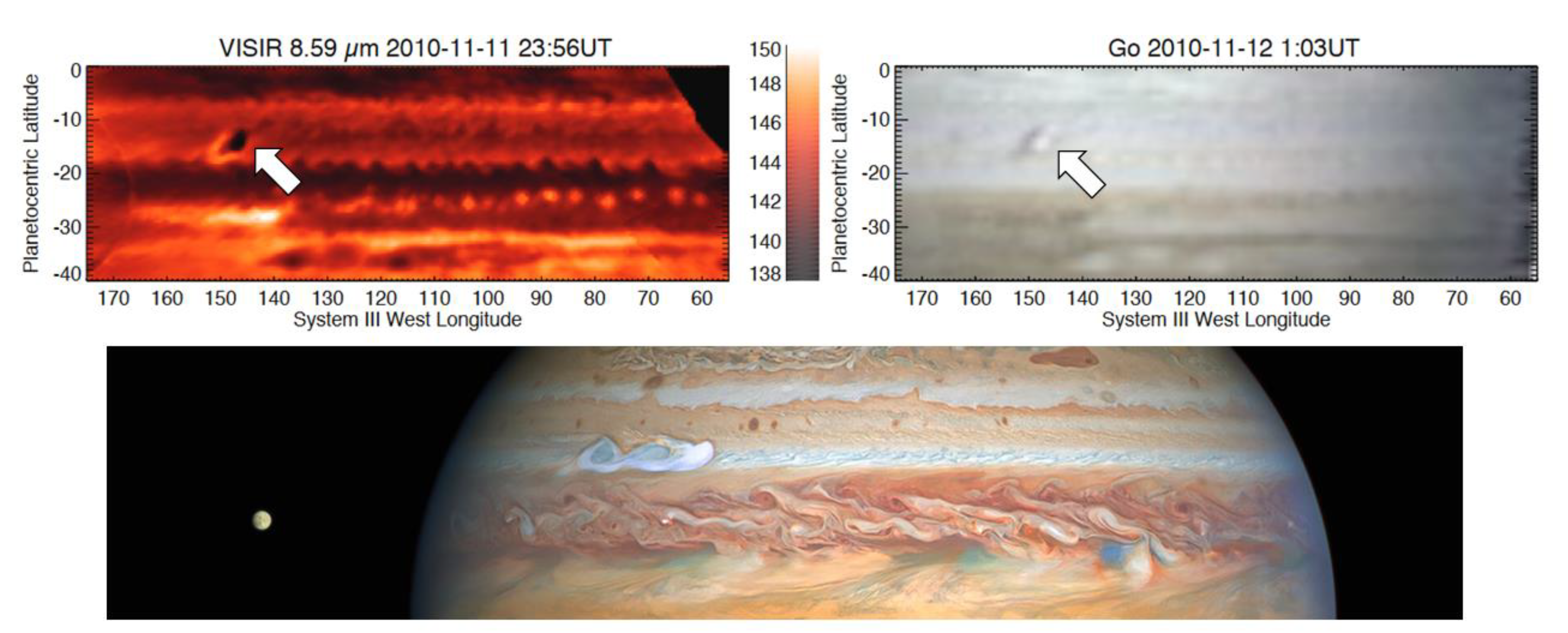
Similarly, in the northern hemisphere, the North Tropical Belt (NTB) to the north of the strongest eastward jet on Jupiter, centered at 24°N (planetographic), has shown periodic convective outbreaks every 5 years, e.g., [30,31]. The initial outbreak is thought to be convective in origin, with the head of the plume generally traveling much faster than the jet [31]. The faster plume head velocity was attributed to the deep source of the outbreak, providing a measure of the wind shear below the visible cloud deck. The plumes themselves reached above the tropopause, pointing a strong convective origin. In the aftermath of the plume, several arc shaped features were observed in the wake of the plume head, which traveled significantly slower than the plume [31]. Modeling efforts attributed these features to an upper level Rossby wave generated from the initial perturbation [32], which featured smaller-scale convective tendencies.

In both cases, observations show a series of disturbances which began with a large white cloud forming from moist convective instabilities (Figure 1). These plumes are bright in the methane band [22] and dark in near and mid-infrared wavelengths [29], denoting that their cloud tops are much higher than the surrounding regions. For instance, Sánchez-Lavega et al. [22] found that the 2007 NTB outbreak had a cloud top pressure of around 60 mbar, showing that the NTB outbreak was powerful enough to overshoot the tropopause (∼100 mb).

However, in both cases, the trigger mechanism for these outbreaks is poorly understood. For the SEB, the belt is characterized by high reflective clouds prior to the outbreak, while the NTB is a low albedo region, making it difficult to use a unified process to explain both instabilities. In the NTB, one possible mechanism is the generation of instability caused by the cooling of upper layers due to the decreased aerosol opacity [15], leading to a convective plume from the water cloud level. In the aftermath of the outbreak, the belt becomes dark in the $5 \mathsf{\mu }$m band, consistent with an opaque upper level cloud cover [33]. While it is known that the SEB outbreak begins with disturbances in brown barges, it is currently unclear as to the role that the cyclonic vortices play in generating these moist convective events.

2.1.2. Cyclone Induced Convection

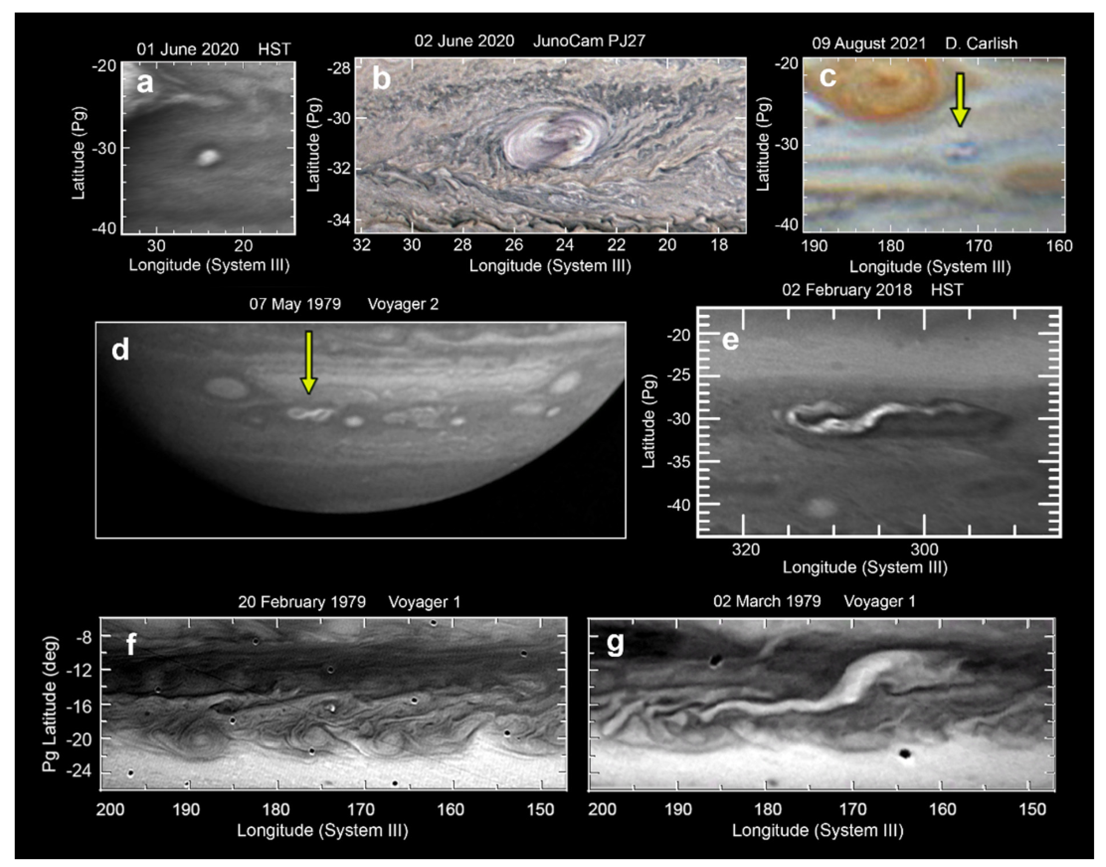
Similarly to these zonal disruptions, large plumes also occur within isolated cyclonic vortices (Figure 2). The Clyde’s spot [34] was first observed by amateur astronomers and the JunoCam instrument as a large white spot in the South Tropical Belt (STB) that formed within a cyclonic barge. Radiative transfer modeling of the feature showed that the clouds are slightly elevated compared to the surrounding STB, and analysis of the divergence of the storm anvil provided constraints on the apparent vertical motion [34]. Over the next several months, the storm developed into a cyclonic system that eventually broke down into a large filamentary structure (Figure 3). These discrete storm systems seem to form sporadically in the STB, nested within cyclonic barges [35], ending up as folded filamentary regions (FFRs) that prevail over several months.

2.1.3. Pop-Up Clouds

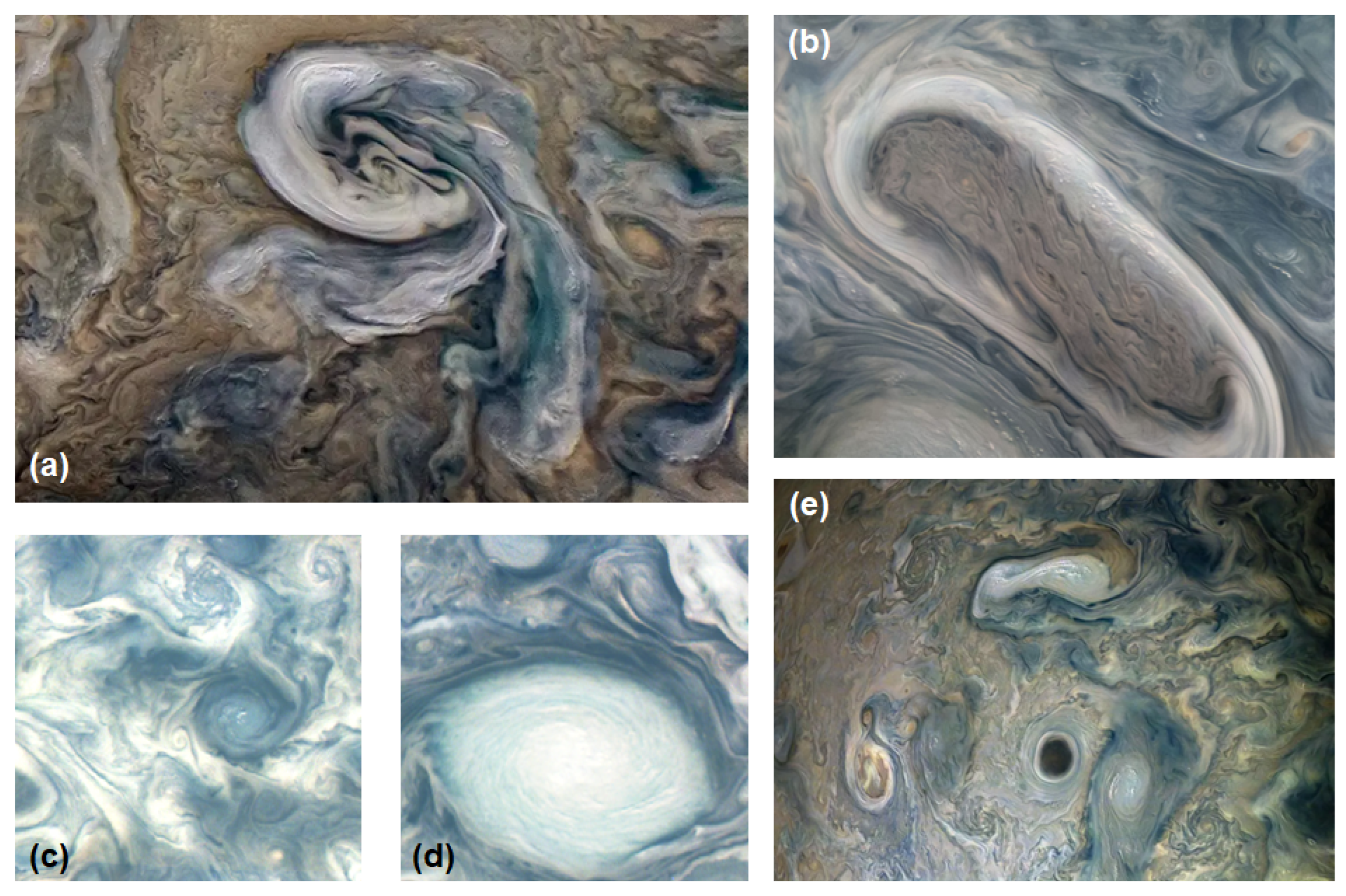
With the higher resolution provided by the JunoCam instrument aboard the Juno spacecraft, smaller-scale convective events were observed within the ammonia cloud deck. These clouds have been extensively imaged by JunoCam but were retroactively identified in some images from the Voyager epoch. These clouds are often termed pop-up clouds (see Figure 4). These do not have the characteristics of large convective plumes detailed above, but some forms share similarity with the altocumulus castellanus clouds on Earth (i.e., tower-like clouds that emanate from a singular cloud base), when arranged in linear/curvilinear forms. When observed as individual clouds or clusters, pop-up clouds appear similar to terrestrial cumulus humilis (i.e., fair-weather cumulus). Pop-up clouds have been identified in a diverse spectrum of environments. A further analysis of the exact nature of these clouds and why they form is currently pending.

Pop-up clouds have been observed displaying several morphologies: isolated individual clouds; clusters; linear/curvilinear; and linear/curvilinear with clustering [36]. The linear/curvilinear forms appear similar to terrestrial altocumulus castellanus clouds [37] and are also quite similar in appearance to linear cloud features observed in terrestrial frontal systems. The linear/curvilinear types have only been observed thus far within folded-filamentary regions and in vortices. The individual and cluster types are typically observed scattered throughout the South Tropical Zone (STZ) and within folded-filamentary regions (FFRs), and sometimes in the interior of vortices. Most of the time these clouds appear bright white, but they have also been observed in the GRS where they appear in the same rust-red shades typically found in that feature.

The vertical location of pop-up clouds within Jupiter’s weather layer suggests these clouds are composed of ammonia ice and probably do not originate from convection seated within the water-cloud layer. Recent analysis conducted on pop-up clouds in the ‘Nautilus’ (Figure 4a) and ‘octopus’ (not shown) features and in other unnamed FFRs indicates that they extend only about 15 km on average above the surrounding cloud deck [36], which supports the hypothesis that these are probably not capable of charge separation that leads to lightning discharges. However, if some pop-up clouds are merely the tops of deep-seated convection, then perhaps lightning may eventually be observed originating within them. To date, optical-identified lightning flashes have not been positively identified to any pop-up clouds, hence they cannot be classified as cumulonimbus based on existing data.

While pop-up clouds have not yet been identified as harboring lightning, they are often found in FFRs, which are frequently associated with lightning as identified in high-temperature spikes in channel 1 of the microwave radiometer, MWR [38]. Juno discovered so-called, shallow lightning, originating at relatively high-altitudes of 1–2 bar. This observation strongly suggests that solid and liquid cloud particles exist even at cold temperatures at these levels in the atmosphere. A phase diagram for water and ammonia demonstrates that such a phenomena is a distinct possibility on Jupiter and Saturn (and more likely on the ice giants) and begs the question if at least some pop-up clouds may contain a similar mixture of solid and liquid hydrometeors. If so, then based on existing observations, the vertical motion of these particles appears to be insufficient for charge separation. However, until periapse is close enough overhead to an FFR during Juno’s Extended Mission for the MWR and/or SRU to distinguish which clouds harbor lightning, it remains to be seen if all pop-up clouds are definitively non-cumulonimbus.

Throughout Juno’s extended mission, periapse will migrate to the nightside hemisphere at northern midlatitudes and polar regions, locations rich with FFRs. During these nightside periapses, overflying FFRs at an altitude of only a few thousand kilometers, the optical low-light Stellar Reference Unit (SRU) camera—which is co-aligned with Channel 1 of the MWR—should be able to determine which clouds are correlated to optical flashes, and, thus if pop-up clouds within FFRs contain lightning. Supporting Earth-based observations taken within a few hours to days of periapse will provide contextual information about the cloud features in case Io- or Europa-shine is not present for the SRU to observe the cloud morphology.

The different morphologies and locations of pop-up clouds associated with zones, FFRs, or in vortices suggest different dynamical mechanisms behind their formation. Some possible mechanisms may involve: slantwise convection; frontal zones encouraging shallow (but mostly vertical) convection; deformation zones squeezing the atmosphere into elongated lines; and perhaps as mundane as day-time heating of the weather layer. This latter mechanism may explain the presence of individual humilis and humilis clusters found within the STZ. Cloud-resolving models applied to these different regions on Jupiter could provide valuable clues for their formation and arrangements, as well as how these small-scale convective clouds influence the larger-scale dynamics and energetics of Jupiter’s weather layer.

2.2. Saturn

Saturn’s cloud structure is similar to Jupiter’s, but given the cooler temperatures, the clouds reside deeper in the atmosphere (for example, water condenses at roughly 10 bars and ammonia at 1 bar [39]). The upper troposphere is dominated by a hydrocarbon haze layer. In contrast to the constant presence of cumulus storms on Jupiter, thunderstorms on Saturn are intermittent.

2.2.1. Local Convective Episodes

Evidence of intermittent thunderstorms on Saturn was first detected during the Voyager flyby of Saturn in 1980–1981. The Voyager spacecraft detected bursts of radio signals, which were believed to have been emitted by lightning discharges within thunderstorms, and were termed the Saturn Electrostatic Discharges (SEDs) [40,41,42,43].

When the Cassini orbiter arrived the Saturn system in 2004, the spacecraft’s Radio and Plasma Wave Science (RPWS) instrument also detected SED signals during the spacecraft’s approach to Saturn before entering orbit [44]. In particular, SED signals were emitted by a series of storms in 35°S latitude between 2004 and 2006 [45,46]. This narrow latitudinal band (known as the “Storm Alley”) is associated with large lightning activity and thunderstorm formation [47]. These storms begin with localized bursts of cloud formation, and eventually form dark ovals. Modeling suggests an upper level extended NH${}_3$ cloud layer forms during the convective stage, rising above the background cloud deck [48]. During the dark oval stage, they function similarly to $5 \mathsf{\mu }$m hot spots on Jupiter, showing reduced aerosol opacity and increase thermal emission from the deeper atmosphere.

Aside from SEDs emitted by the Storm Alley, notable other SED episodes include a sizable storm observed around 70°N in 2018 [49], which is the largest convective event that has been observed to date other than the Great White Spots described in the next subsection and also the highest-latitude thunderstorms that have been seen to date. Another notable event is a series of storms observed in the 50°N latitude between 2010 and 2013 [50] that disrupted a cyclonic vortex in which the storm is believed to have injected anticyclonic vorticity and dissipated the cyclonic circulation in the vortex.

2.2.2. Great White Spots (GWSs)

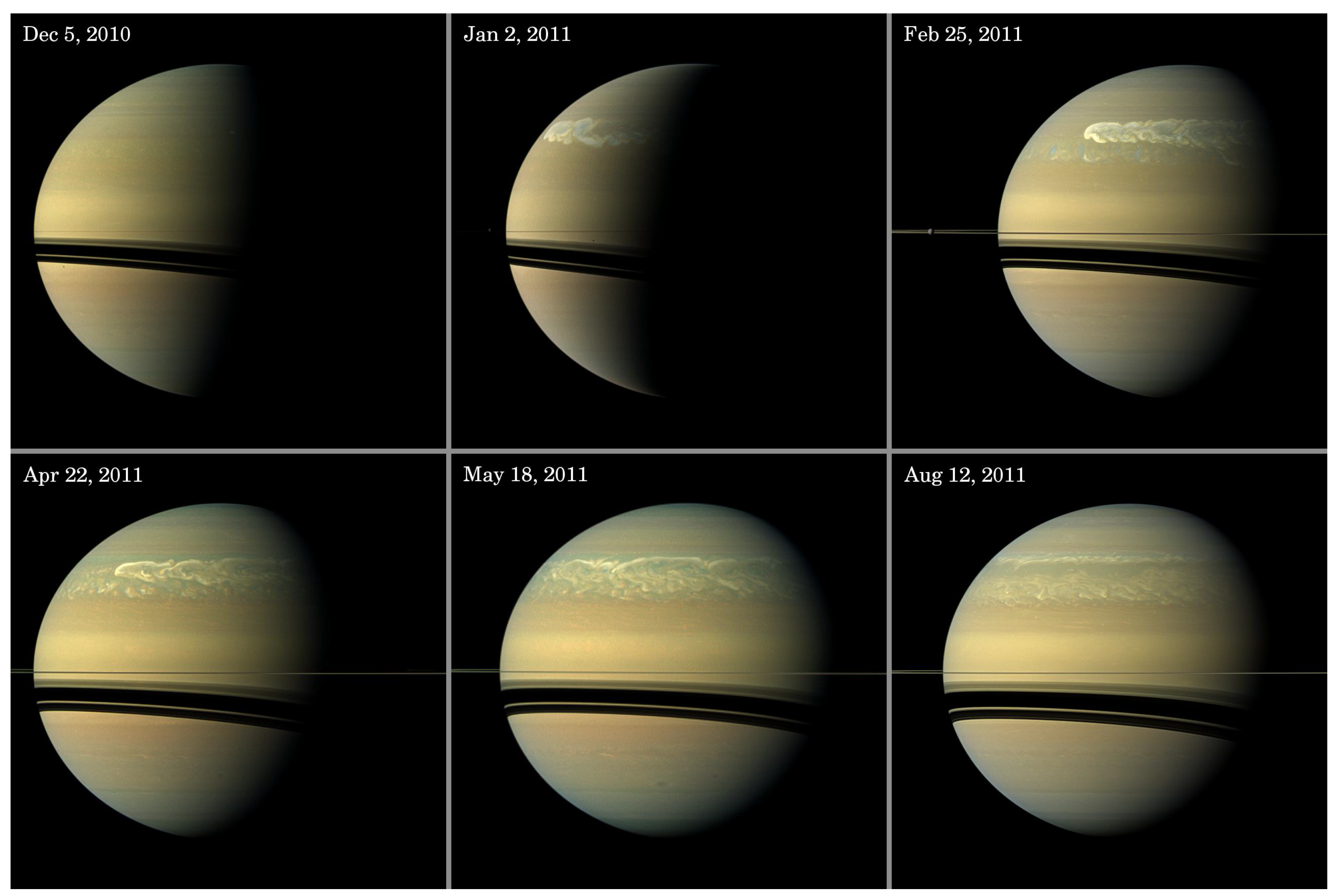
The most intense episode of SEDs was observed during the 2010–2011 Great Storm of Saturn [51]. The 2010–2011 storm is believed to be the latest occurrence of the giant storms that repeat on Saturn approximately every 30 years, previously observed in 1876, 1903, 1933, 1960 and 1990 [52]. From Earth, these storms appear as a spot of particularly bright clouds that last for many months and thus have historically been called the Great White Spots (GWSs). These giant storms last for many months and are the true exceptions on Saturn where thunderstorms are mostly absent. The 1990 storm erupted while the then-new Hubble Space Telescope (HST) was being calibrated, and became HST’s first scientific observation and documented the temporal evolution of the cloud evolution in detail [52,53]; the storm motivated several numerical modeling studies to examine the dynamics of such storms [54,55]. The 2010–2011 storm occurred while Cassini was orbiting Saturn, and allowed detailed observations of the storm’s cloud morphology as well as SED signals to reveal that intense cumulus storms continuously erupted for over 6 months [51,56]. The high spatial resolution observations by HST and Cassini showed that the bright clouds produced by the 1990 and 2010–2011 storms encircled the entire latitude bands of the storm and altered the structure of the atmosphere at that region (Figure 5). Detailed review of the 2010–2011 storm is presented by Sanchez-Lavega et al. [57].

Radiative transfer modeling of the storm using Cassini VIMS data showed that the spectra could be fit well by a water cloud with significant opacity up to the 1 bar level, with a possible optically thick ammonia cloud deck above the 1 bar level [58]. The water cloud was several scale heights tall, and lightning was frequently observed using the Cassini Radio and Plasma Wave Science (RPWS) instrument [51], denoting the storms’ convective origins in the water cloud base. Much like the STB revival on Jupiter, this storm originated in a series of cyclonic vortices (named the ‘String of Pearls’ [59]).

The 2010–2011 storm was also notable in altering Saturn’s total thermal emission. Like Jupiter and Neptune, Saturn emits more energy in the form of thermal radiation than it receives from the sun [60,61]. The excess heat is primarily emitted from tropospheric layers, which in turn receives heat from the deep warm interior through thermal convection; in the tropospheric layers, cumulus convection is believed to be primarily responsible for the vertical heat transport. IR observations showed a stratospheric ‘beacon’ (a positive thermal anomaly) in the wave of the GWS. The beacon was likely a result of gravity waves generated by the convective activity breaking at the tropopause, and injecting energy into the stratosphere [62]. During and after the 2010–2011 giant storm on Saturn, Saturn’s total emitted power increased by about 2 percent [63], hinting that the thermal balance of Saturn may be driven by episodic events like GWSs. The highly episodic nature of these storms may be regulated by the fact that the molecular mass of the main condensable species, namely water, is heavier than the average atmospheric molecular mass primarily made of hydrogen gas [64].

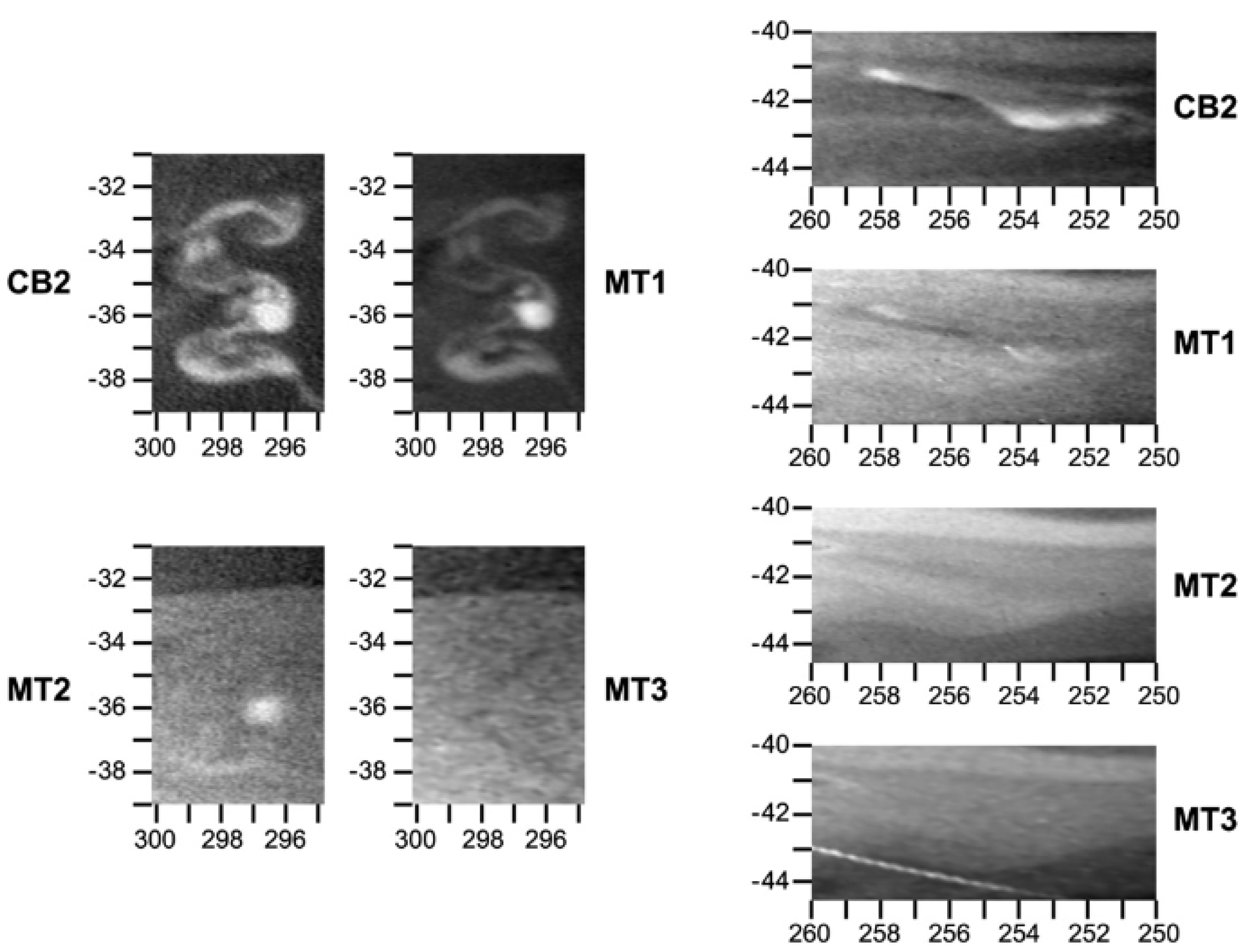
After the 2010–2011 storm, the storm activities on Saturn returned to the intermittent state. Cassini images reveal several smaller cloud structures that were bright in the visible wavelengths (Figure 6).

2.3. Uranus

Uranus has far fewer discrete cloud features than Jupiter, Saturn and Neptune. The upper atmosphere is dominated by a thick haze, while CH${}_4$ forms sporadic, but optically thick clouds near the 1 bar level [39]. Below the CH${}_4$ clouds, there is evidence of an optically thick cloud deck, thought to be composed of H${}_2$S [66]. While reports of sporadic spots date back to 1870 [67], historically, Uranus was not known to harbor features that could be tracked from Earth. The Voyager 2 flyby of the planet did not significantly change this view; although a later reanalysis [68] identified dozens of features not initially detected [69], this only spacecraft flyby of Uranus to date confirmed the dearth of discrete clouds on the planet. Lightning was detected during the flyby using high frequency radio observations (called the Uranian Electrostatic Discharge; UED), hinting at deep convective activity [70]. UEDs were thought to originate in the water cloud layer, which are too deep to observe directly [39,71]. Follow-up on lightning detection has been difficult from ground-based observations, however, and future spacecraft missions hold the key in understanding the processes governing atmospheric electricity on Uranus.

Later observations by HST resolved some cloud features that were tracked for long enough to enable zonal wind measurements [72,73]. One feature that appeared to have lasted at least since the Voyager 2 flyby in 1986 until 2009 known as the Berg is likely vortical in nature while it may also have triggered cumulus storms [74,75,76]. While Uranus does not totally lack discrete clouds, these reports that discuss detection of discrete cloud features on Uranus underscore the challenges and rarity of these cloud sightings.

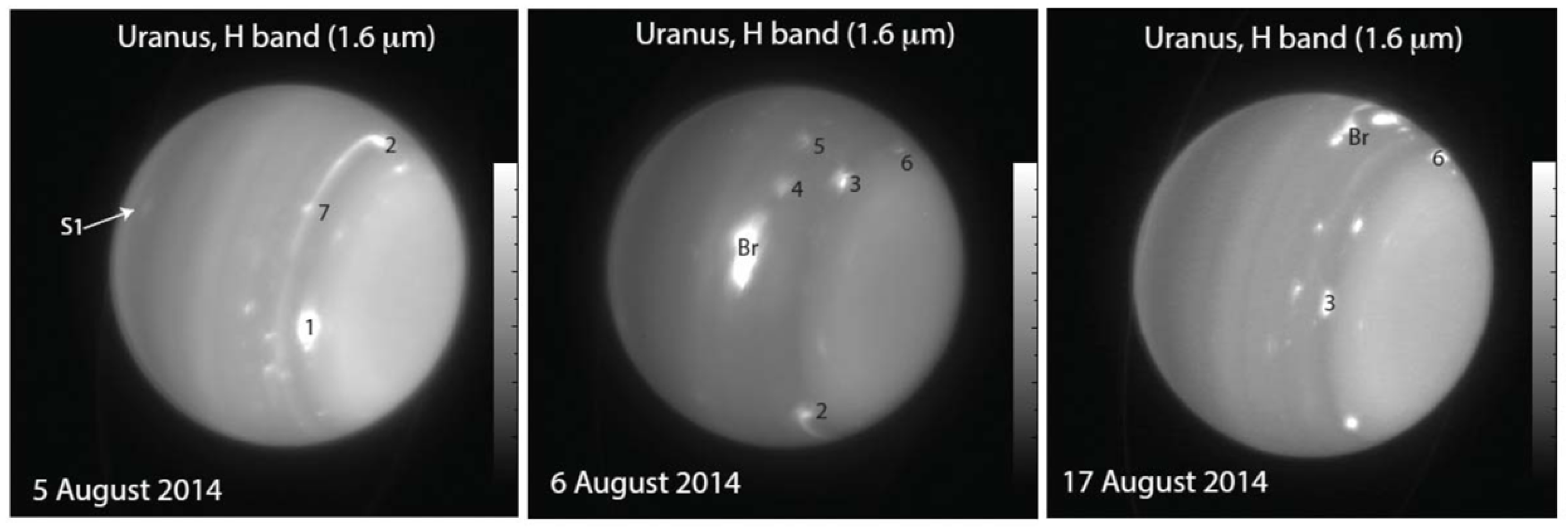
As Uranus approached the 2007 equinox, detection of temporally variable cloud activities significantly increased aided by the advent of modern large telescopes equipped with adaptive optics (AO). The first such detection was made in 2004 using the Keck telescope [77], and more reports of temporally dynamic clouds followed during and after the equinox [74,75,78,79] (Figure 7). Even though detection of these new clouds roughly coincided with the introduction of AO systems, multiple full-longitude observations by HST and Keck starting in 1997 showed that Uranus was much less active until 2004 [72,73,80,81,82]; thus, the increased cloud variability since 2004 is interpreted as a sign that Uranus has entered an active period. At least some of these temporally variable clouds are believed to be cumulus in nature because of their rapid evolution.

Curiously, during the Voyager 2 flyby of Uranus, the planet was not seen to emit excess heat, which is unlike Jupiter, Saturn and Neptune [60,61]. Considering that Saturn’s thermal emission increased following its 2010–2011 Great Storm [63], the fact that Uranus was in approximate thermal balance (i.e., the planet was emitting the same amount of heat that it was receiving from the sun) in 1986 may be related to the absence of observable clouds during the period. One possibility is that Uranus releases its internal heat only during an active period. Due to Uranus’ cold atmosphere, water is expected to condense at the depth of 200 bar level [83], and any cumulus convection originating in the predicted layer of supersaturated water vapor would need to overcome the strong stabilizing effect of the relatively heavy water molecules [84,85,86]; thus, such storms may erupt in a manner even more episodic than the GWSs on Saturn. This need to understand the thermal evolution of Uranus should serve as a strong motivation to realize an orbital mission in the near future to test whether the planet emits more internal heat during the ongoing active period than during the 1986 Voyager 2 flyby.

2.4. Neptune

Due to Neptune’s great distance from Earth, resolving discrete features on the planet is a significant challenge; nevertheless, visual reports of clouds date as far back as 1948 [87,88]. Even before Neptune could be resolved by imaging instruments, photometric observations regularly showed variable reflectivity of the planet, which was interpreted to be caused by discrete clouds coming in and out of sight as the planet rotated [89,90,91].

Modern CCD imaging observations enabled resolving these Neptunian clouds as first reported in 1979 [92,93]. The concerted efforts to observe Neptune to support the Voyager 2 flyby in 1989 further demonstrated that discrete features are regularly present on Neptune [94,95,96,97]. The Voyager 2 flyby itself found many clouds, some of which varied in a timescale of hours, while also revealing the details of the largest features which were detected from the ground such as the Great Dark Spot [98,99,100]. Detection of radio signals that resembled whistlers during the Voyager 2 flyby are also interpreted to be evidence of lightning in Neptune’s atmosphere [101].

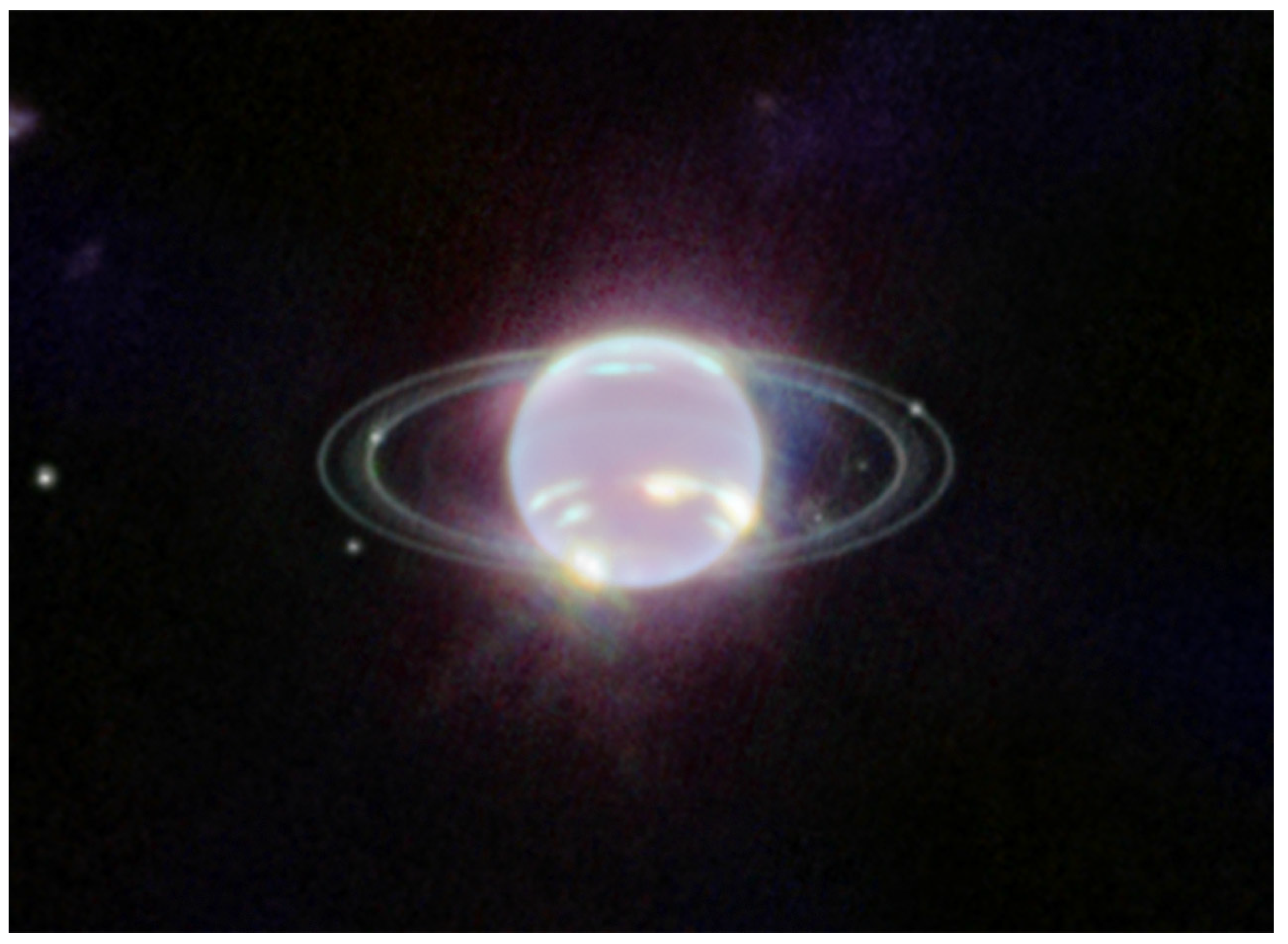
Neptune’s atmosphere continues to be highly active to date including formations of a new dark spot [102], an equatorial storm [103] and other smaller features [104,105,106]. Mid-infrared observations of the planet also reveal that stratospheric temperatures exhibit changes in timescales shorter than a season, which may be driven by cumulus events in the troposphere [107]. One of the first images returned by NASA’s recently launched James Webb Space Telescope captured the clearest view of Neptune since the 1989 Voyager 2 flyby, and promises to bring potential to further understand Neptune’s high atmospheric variability [108] (Figure 8).

Combined with the measurement of the fastest zonal wind speeds on any solar system planet, the prevalence of active clouds was a surprise at the time of the Voyager 2 flyby [98]. However, Voyager 2 also showed that, among the four solar system giant planets, Neptune emits internal heat at the highest rate relative to the absorbed solar energy [60,61]; thus, perhaps these storms are driven primarily by the release of the planet’s internal primordial heat. Nevertheless, the causal connection between the presence of active clouds and high internal heat release remains unclear—perhaps the internal heat is transported to the troposphere at a high rate and drives the observed regular cloud activities, or, alternatively, perhaps Neptune’s current high thermal emission is due to the planet undergoing an active period of cumulus storms. Note that Neptune has completed only a quarter of its 165-year orbit since the first CCD detection of resolved clouds in 1979, and less than half an orbit since the first visual reports of discrete features in 1948. Any study of seasonal-scale variation would require many more decades of regular monitoring from Earth as well as multiple orbital and flyby missions.

3. Dynamical and Microphysical Processes in Convective Storms

3.1. Cloud Microphysics: Lifetimes of Condensates in Planetary Atmospheres

The formation and evolution of a cumulus storm cell is governed by the vertical structure of the atmospheric temperature and aerosol concentration. Cumulus growth is enhanced by the presence of an (moist) adiabatic atmospheric lapse rate, which in turn, requires a sufficiently saturated atmosphere. Cloud particle growth depends on the type of particle, which varies based on the background atmospheric properties (e.g., pressure, temperature) and origin of the particle. Generally, cloud particles are activated either heterogeneously (condensation occurs on a small foreign particle, i.e., cloud condensation nuclei, or CCN) or homogeneously (i.e., cloud species molecules join and form a cloud embryo without the presence of a CCN), with the latter process being less efficient, and thus resulting in fewer particles. From the embryo, cloud growth is dictated primarily by condensation and collection, while precipitation acts to remove particles from the cloud.

1.

Condensation/Deposition: Condensation is the process whereby moisture from the vapor surrounding the particle condenses directly on to the particle. For a super-saturated environment, the vapor will readily condense on the surface of the cloud particle, allowing for quick growth from the initial embryo. Given a constant ambient supersaturation, the rate of cloud size growth decreases with radius, thereby making this process very inefficient in generating large particle sizes. For Earth and even for Gas Giant atmospheres, condensation is primarily responsible for particle sizes up to $\lesssim 1$ $\mathsf{\mu }$m. For ice particles, the same process occurs, but the liquid phase is skipped, and vapor is directly deposited as ice on the particle.

2.

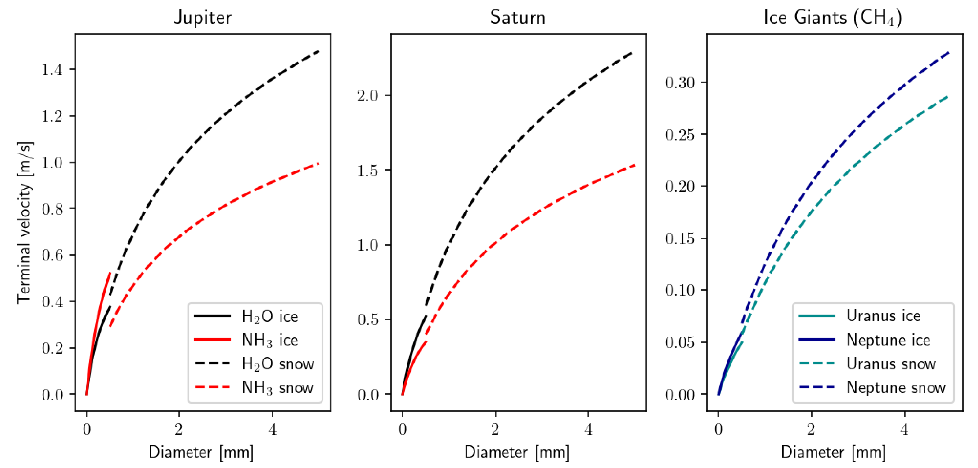
Precipitation: Due to the small sizes of the particles, they quickly reach terminal velocity, and fall as they continue to grow. The terminal velocity of the particle depends on the shape and phase of the particle, and generally increases quickly with particle radius. Very small particles ($r \lesssim$ 1 $\mathsf{\mu }$m) fall very slowly, and thus clouds with such particles are generally treated as ‘non-precipitating’, with precipitation generally describing only larger particles ($r \gtrsim$ 250 $\mathsf{\mu }$m) [109], whose terminal velocities reach on the order of cm/s to m/s. The shape of the particle (especially for ices), drastically affects the hydrodynamics of the particle, and larger particles deviate strongly from the Stokes regime [110]. Smaller particles (≲1 $\mathsf{\mu }$m) usually have high Knudsen number, and thus require the Cunningham correction [111]. Therefore, throughout the lifetime of a hydrometeor, the flow around the particle may pass through several different flow regimes. The typical terminal velocity profiles of cloud ice and snow particles in Solar System gas giants are shown in Figure 9. See Loftus and Wordsworth [112] for a detailed analysis of raindrops in planetary atmospheres and Guillot et al. [113, 114] for mixed-phase solid particles.

3.

Collection (coagulation/aggregation and coalescence): Growth beyond the 1 $\mathsf{\mu }$m sizes occurs primarily through collisions and sticking between different particles. As particles grow, so too does their terminal velocity, and thus, larger particles will generally fall through a field of smaller sized particles. The sticking efficiency, usually denoted by $E(r,r^{\prime })$, describes the probability of two particles of different sizes r and $r^{\prime }$ being able to constructively collide to form a larger particle. Sticking efficiency is usually a complicated function of the difference in velocities, the mechanical properties of species of the two particles (e.g., surface tension) as well as the nature of particles (ice/liquid). However, in general, sticking efficiency increases with the size of the particle, leading to a runaway growth in particle size, as long as there is sufficient cloud mass for a particle (now called a ‘hydrometeor’) to accrete. Coalescence is the process where smaller particles are absorbed into the larger particles due to the latter falling through a ‘field’ of smaller hydrometeors, while coagulation/aggregation refers to the process where nearly equally sized particles merge due to chance collisions from Brownian motion. Justifiably, coalescence dominates for larger particles, while coagulation is more efficient in the small radius regime.

The growth rate of a particle is dictated by the efficiencies of the above processes. In a supersaturated environment, the particle will generally follow the fastest growth process forward (i.e., vapor is condensed/deposited onto the cloud), whereas in a subsaturated environment, the particle is more likely to evaporate/sublimate. Precipitation (given by the magnitude of the terminal velocity) becomes important when the particle is carried away from the source to a drier region faster than it can grow.

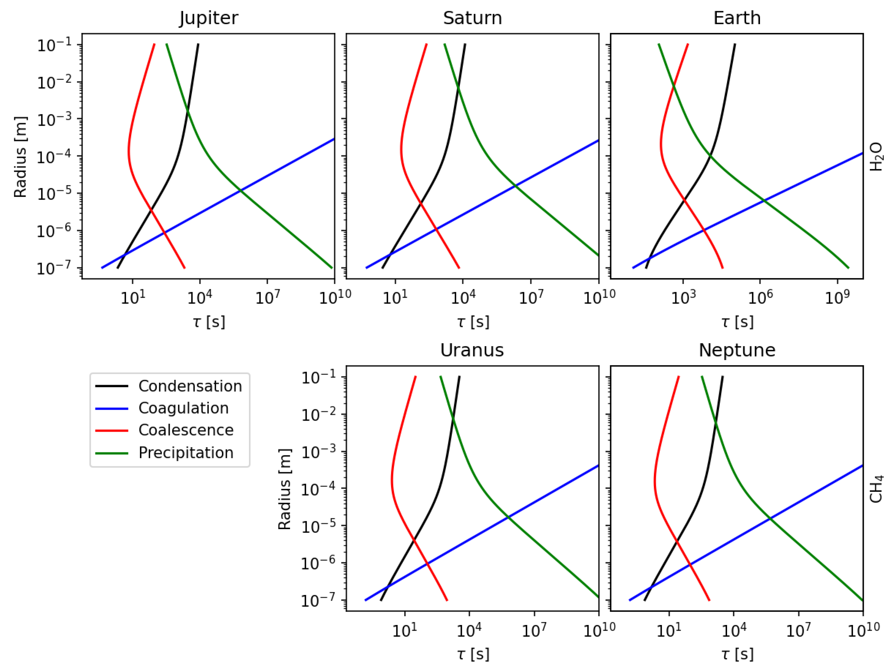
A simple mechanism for understanding the competition between these processes is to look at the typical time taken to create (or dissipate) a particle of a given size [115,116]. Figure 10 shows characteristic timescales for water ice on Jupiter, Saturn and Earth, and methane ice on Uranus and Neptune. Formation processes (condensation, coagulation, coalescence) are initially much faster compared to precipitation for small particles, and thus condensation can quickly grow initiated particles, within a few seconds, to a size of ∼1 $\mathsf{\mu }$m. Beyond this, coalescence helps the particles grow to ∼1 cm through collisional mergers, at which point precipitation timescales become short enough to carry the particles away from the source and inhibit growth. All the examples shown here demonstrate particles large enough to precipitate forming within the timescale of a few hours ($\tau \sim \mathcal{O}\left({10}^4\mathrm{s}\right)$), which is comparable to the time scale for thunderstorm formation in the tropics on Earth.

Planetary clouds are inherently difficult to model, though, since they form in a wide diversity of thermal and dynamical regimes. Early studies of planetary clouds used equilibrium considerations to determine locations of clouds [71]. While this did not provide an estimate of the cloud particle distributions, it did provide an estimate of the vertical locations of high cloud condensation efficiency [7]. For more dynamically forced clouds (e.g., in convective storms) (Ackerman and Marley [117] and derivatives) model these microphysical processes in a 1D atmospheric column by parameterizing the vertical mixing, and analysing the steady state cloud structure for different vertical mixing regimes. Currently, more sophisticated microphysical models, e.g., Ohno and Okuzumi [118], Barth [119] fully model the microphysical processes of cloud formation to study the dynamical evolution of clouds over time. Such studies are valuable in inferring and disentangling cloud formation on these planets over a wide swath of dynamical regimes. Nevertheless, such models are computationally intensive, and a comprehensive treatment of the microphysics of cloud formation in retrieving aerosol structures from observations is inherently challenging, albeit a necessary next step in studying planetary atmospheres.

3.2. Dynamics of a Convecting Parcel

In general, moist convection occurs in the atmosphere when the lapse rate (i.e., rate at which temperature decreases with altitude) of the environment is greater than the lapse rate that a rising moist air mass is experiencing, creating a parcel-environment instability. This process can be described using simple parcel theory, e.g., Emanuel [120] envisioning a control volume containing a humid air parcel (e.g., H${}_2$O in the case of Earth). As the moist parcel ascends, it will expand adiabatically and cool at the dry-adiabatic lapse rate until condensation occurs at the lifting condensation level (LCL). Latent heat is released and the parcel now cools at the moist-adiabatic (wet-adiabatic) lapse rate. If the triggering mechanism is sufficiently energetic the parcel might ascend to reach the level-of-free convection (LFC), where the parcel becomes less dense than the surrounding gas, and becomes unstable to convection. As the parcel continues to rise and condense, it will dry up and eventually becomes denser than the surrounding gas, becoming negatively buoyant at the equilibrium level (EL).

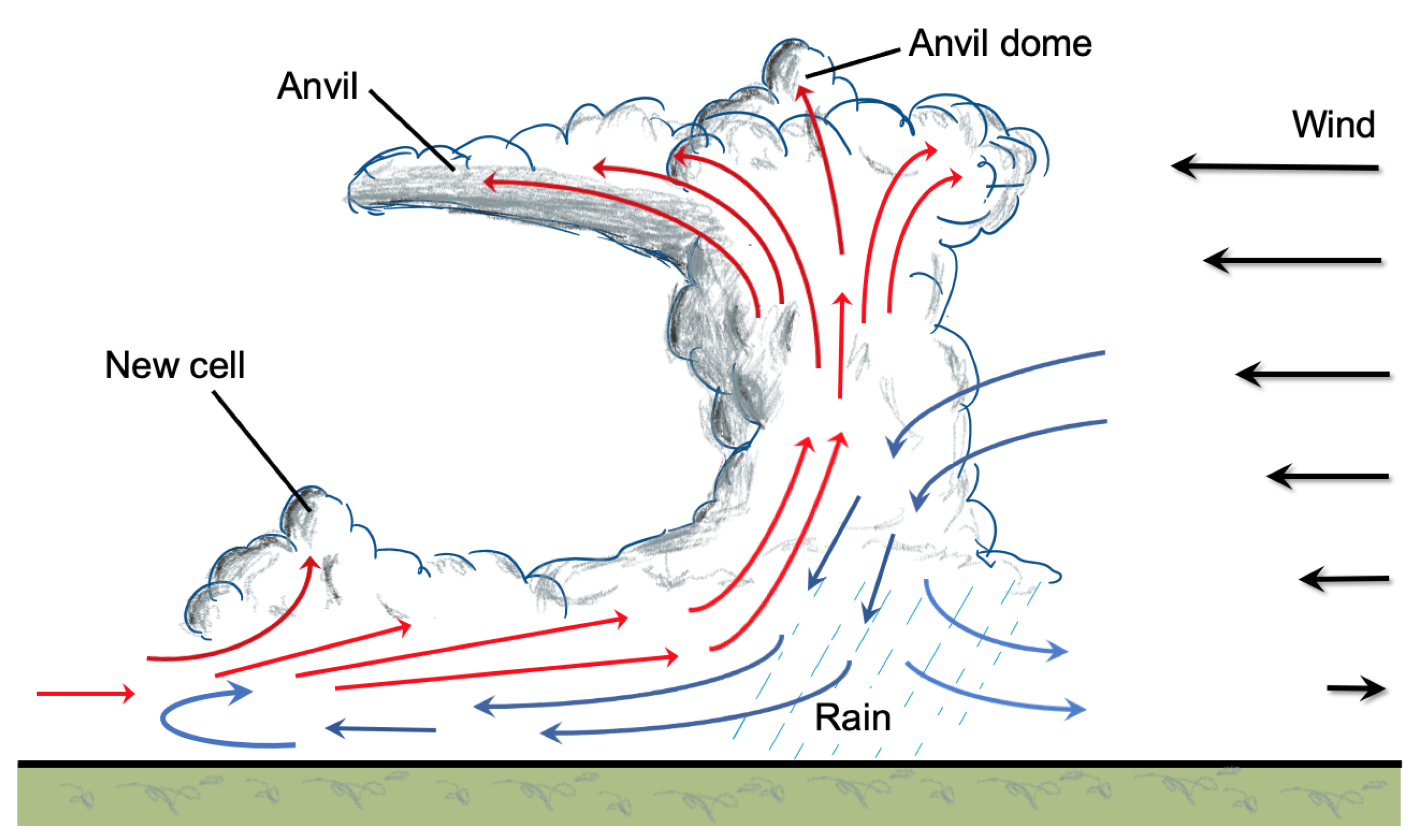
At the EL, the vertical velocity of the parcel reduces to zero and it can no longer ascend. At this stage, the top of the convective plume is forced to spread out horizontally into an anvil shaped cloud. Parts of the parcel, however, maintains some of its vertical momentum and overshoots the equilibrium level, creating a bulge on the top of the anvil that is called anvil dome or penetrating top. This dome exerts an upward force on a stable air layer above it, most often creating gravity waves in that process that reshapes the top of the cloud when viewed from above. In planetary exploration, these types of clouds can be used to diagnose convective features below the cloud tops that otherwise may not be identifiable.

The total energy released by the parcel during this free convection region is called the Convective Available Potential Energy (CAPE), and is given by the integral of the total positive buoyant forcing experienced by the parcel,

$$\begin{array}{c}\hfill \mathrm{CAPE}={\int }_{z_{\mathrm{LFC}}}^{Z_{\mathrm{EL}}}g\left(\frac{T_{\mathrm{v},\mathrm{parcel}}-T_{\mathrm{v},\mathrm{env}}}{T_{\mathrm{v},\mathrm{env}}}\right)dz,\end{array}$$

(1)

where $T_{\mathrm{v}}$ is the virtual temperature (a combination of kinetic temperature and saturation vapor and pressure effects), g is the gravitational acceleration, and $Z_{\mathrm{LFC}}$ and $Z_{\mathrm{EL}}$ are the altitudes over which the parcel rises. Subscripts $\mathrm{env}$ and $\mathrm{parcel}$ denote the ambient atmosphere and parcel, respectively.

Conversely, until the LFC, the parcel will generally experience negative buoyancy during the ascent. Therefore, to reach the LFC, the parcel must be forced up, and convection can only happen when the kinetic energy from forcing is stronger than the Convective Inhibition (CIN), given by the total negative buoyancy experienced by the parcel from its initial location up to the LFC,

$$\begin{array}{c}\hfill \mathrm{CIN}=-{\int }_{z_0}^{Z_{\mathrm{LFC}}}g\left(\frac{T_{\mathrm{v},\mathrm{parcel}}-T_{\mathrm{v},\mathrm{env}}}{T_{\mathrm{v},\mathrm{env}}}\right)dz.\end{array}$$

(2)

If the initial forcing is sufficiently strong (at least as high as the CIN), the parcel ascent will generate a convective storm reaching up to the EL. As the moist air mass rises within the storm, drier environmental air is entrained into the updraft mainly from its side via turbulent eddies. Storms with larger horizontal cross sections are less affected by this process as the core of the updraft is far enough from its edge to be reached by the entrained air, while narrower storms experience more damaging effects from the mixing of colder environmental air [121]. The genesis and evolution of these storms depend on the thermodynamic stability of the background atmosphere, the vertical wind shear, forcing conditions, among other factors. The required environmental properties also depend on the type of the convective event, whether it comprises a single convective cell, a multicell storm or a cluster of cells, squall line (i.e., multicell line), a supercell, or larger-scale system containing individual cells such as Mesoscale Convective Complexes (MCCs). Even on Earth, the exact nature of these forces is not well understood and is indeed thought to be a combination of several processes acting in tandem [122].

The vertical wind shear of the background atmosphere also has a strong effect on how the convective cells evolve, the shape of the storm and the motion of the air within (Figure 11). Smaller storms may get torn apart by strong vertical wind shear, preventing their growth and limiting their lifetimes, while the growth of larger convective features may benefit from a strong shear [123]. In single cell convective storms, as soon as the precipitation particles become too heavy to be kept aloft by the updraft they begin to fall and initiate the downdraft. The evaporating condensates in the downdraft increase its strength and it spreads out horizontally upon colliding with the surface. The precipitation and the diverging downdraft at the surface are two characteristics of the dissipating stage of the storm.

Fundamentally, convective storms on the giant planets should be analogs to their terrestrial counterparts and in many aspects they are, but there are some key differences. The inclusion of condensable species (i.e., water) on Earth reduces the mean molar mass of moist air, while on the gas giants the opposite is true. The background atmosphere is mainly a hydrogen-helium mixture and the condensable species of ammonia (NH${}_3$), ammonium hydrosulfide (NH${}_4$SH), water (H${}_2$O), hydrogen sulfide (H${}_2$S), or methane (CH${}_4$) increase the mean molar mass of air. The resulting structure of the atmosphere is very stable and high abundance values of the condensable species actually inhibit convective motion [64,84,85,124].

The latent heat of condensation of a particular species and the abundance of vapor that is available to form condensates strongly affect whether convection is possible and if so what the strength of the resulting storm is. For example, pure ammonia clouds on Jupiter and Saturn are unlikely to form large convective cells, while methane and water clouds on the ice giants and water clouds on the gas giant have the potential to create heavily-precipitating clouds and convective features [116]. This is one reason why it is thought that the convective storms on the gas giant planets originate at the water cloud level and penetrate through the ammonia cloud deck (e.g., [125]). These storms may have a vertical extent of more than 50 km and updraft speed of more than 100 m/s, both of them significantly greater than the same parameters of a terrestrial storm. Observations of lightning in the deeper layers of the atmosphere are also consistent with convective storms originating at the water cloud level.

Many of the observed storms on the giant planets reach a horizontal size of thousands of kilometers, thus it is unlikely that these events are single-cell storms. Additionally, single-cell storms have a relatively short lifetime so they never exhibit a quasi-steady state that some storms on the giant planets display. On Earth, the outflows created by the downdraft often trigger the onset of new convective cells (Figure 11), increasing the spatial and temporal extents of these storms. In the absence of a planetary surface this process cannot take place on the giant planets but it can be replaced by the convergence of multiple moist air masses at depth [126] that also has the potential to trigger additional convection cells. This mechanism is poorly understood and requires more thorough analysis, possibly through modeling efforts, e.g., [127].

3.3. Effects of Convection on Cloud Particle Growth

Within a cumulus updraft, cloud evolution is dictated by the relative intensities of the above processes occurring over a range of altitudes. The growth trajectory of a single hydrometeor is a complicated function of the dynamics of the cumulus cloud and the ambient environment. Generally speaking, initiation of cloud particle within a cumulus updraft will work the same as described above, except for the fact that the updraft carries moisture-rich vapor upwards, resulting in cooling and more efficient condensation.

The initiated cloud particle will continue to grow as it is lofted upwards, as the decreasing temperatures promote condensation, while the increasing release of latent heat drives the ascent of the cloud parcel, until the particles reach enough size for collection to become an efficient method of growth. In this stage, the primary difference between the description above, is in the fall speed of the hydrometeors. Due to the presence of an updraft, only particles that have terminal velocities larger than the updraft velocity will fall downwards, whereas the rest will move upwards with the flow [128]. Therefore, small particles with low terminal velocities (≲1 m/s) will spend considerably more time in the cold moisture-rich environment that is conducive of growth, compared to particles that form in stratiform clouds (where updraft speeds are negligible). This greatly promotes cloud growth and allows a longer timescale for the cumulus cloud to evolve and grow, as long as there is sufficient moisture mass and energy in the initial trigger to support convective updrafts during this stage.

Generally, temperatures in the upper regions of the cumulus updraft are well below freezing, and thus quickly initiate ice particles. If the particles begin from a warm (above freezing) environment, these particles usually begin as small liquid droplets which remain liquid even at below freezing temperature (i.e., ‘supercooled’ droplets), which freeze instantly on contact with other supercooled particles. This mechanism allows for quick growth of large ice particles in the upper regions of the cumulus updraft [129]. Throughout the entire duration of cloud particle growth, latent heat release helps to further drive and sustain the updraft.

Finally, once particles are large enough to not be supported by the updraft, they will fall as precipitation, with the shape of the precipitation being dictated by the particles’ formation histories and the coalecense that occurs as they merge with other particles on the way down (e.g., rain for ‘warm’ clouds, snow for cold clouds, graupel for mixed-phase). Within the cumulus cloud, the largest particles are initially near the top, due to the reasons detailed above. However, as they descend, these particles also experience warmer temperatures and begin to evaporate, leading to atmospheric cooling. This precipitative cooling disrupts the updraft and leads to a dissipation of the cumulus updraft. The timescale for this disruption depends on the initial updraft strength and the source of moisture.

3.4. Types of Cumulus Convection

Cumulus convection, a subset of moist-convection, can be defined when condensation or deposition of a vapor occurs in a cloud with a ratio of vertical to horizontal extent of $\sim \mathcal{O}$ (1) with a concomitant release of latent heat. The vertical to horizontal ratio of cumulus convection differs from stratiform moist “convection” where the ratio is $\ll \mathcal{O}$(1). Cumulus clouds occur with a variety of sizes, from the familiar terrestrial “fair-weather” cumulus-humilis and cumulus mediocris of limited vertical extent, through the intermediate-height cumulus-congestus, to the tall electrically-discharging thunderstorm cumulonimbus clouds [130]. All, however, form from air ascending with a significant vertical component motion as in a buoyant plume. In short, cumulus convection does not necessarily equate to lightning generation but lightning generation in a giant-planet’s atmosphere requires sufficiently strong cumulus convection. Given the spatial and temporal coverage of various spacecraft and the variety of instrument types onboard, the non-detection of lightning does not necessarily indicate that strong cumulus convection or lightning discharges are not occurring. It may simply be an example of insufficient coverage or instrument capability to detect lightning in a given environment (e.g., non-detection of visible light flashes on the dayside hemisphere).

Not all cumulus convection is the same, however; some cumulus storms are temporally and spatially limited, from a few km to a few dozen km, whereas others can be long-lived and larger, a few hundred to a thousand or more km, organized into systems containing multiple individual cells, e.g., [12,125]. In some outbreaks, cumulus convection can significantly change the characteristics of nearby jets (e.g., [32]), alter a portion of a belt or zone (e.g., [35]) or affect belts or zones on a planetary scale (e.g., [15,52,55]). These larger organized cumulus systems are termed mesoscale convective systems MCS, one such category is a mesoscale convective complex MCC (e.g., [131,132]). These convective systems can affect the local environment such that they can sustain themselves longer than small individual cumulus storms. Observations and numerical modeling of Jovian cumulus convection clearly shows the development of storm systems as MCCs [133]. The sizes of these complexes may become close to the same scale as the Rossby deformation radius, $L_D=\frac{NH}{f}$, where N is the Brunt-Väisälä frequency and H is the atmospheric scale height. $L_D$ is a typical scale for the peak growth rates of baroclinic instability, and this scale should be reflected in turbulent power spectra if baroclinicity is involved (see the following section).

4. Convective Energy Cascade

Long cadence observations of the gas giant planets have shown a variety of convective processes. These process function over a vast range of energies, as detailed in Section 2. Convective events appear to be driven by internal heating within these planets, where the build-up of internal heat below the atmosphere leads to the formation of instabilities over time [134]. Radiative cooling to space from the upper troposphere appears to also play an important role in triggering convection as detailed in [64,133]. Latent heat release from these convective storms appear to generate a large fraction of the internal heat from these planets, and thus these storms seem to be major component in the transport of the internal heat to the upper atmosphere [125]. Numerical simulations show that the latent heat release from water is sufficiently high to match observations of the size and scale of convective outbreaks [18,135].

The different planets appear to have different timescales over which convective storms form. For example, Jupiter has several convective outbreaks in the 4–8 year timescale [33], while Saturn produces a massive outbreak (dubbed the Great White Spot; see Section 2.2.2) every 30 years [49]. The ice giants do not seem to demonstrate a regular periodicity, although this may due to limited observations and in-situ data from these planets [136]. Li and Ingersoll [64] showed that the timescales for convective events in H-He atmosphere is driven by the molecular weight gradient and the radiative cooling in the upper atmosphere. For Jupiter and Saturn, convective events driven by water provide a way to measure the water abundances on these planets [18,64,124]. For the ice giants, this gets much more complicated due to inhibition of convective activity (i.e., increase in CIN) due to double-diffusive convection [84,85] and the depletion of water upto very high pressures. Understanding the mechanisms for heat transport in these atmospheres is vital for constraining both the chemical abundances as well as answering key questions about the convective dynamics at play. One avenue is to investigate the features that result from convective outbreaks, and transfer of energy from local convective events to the global scale dynamics.

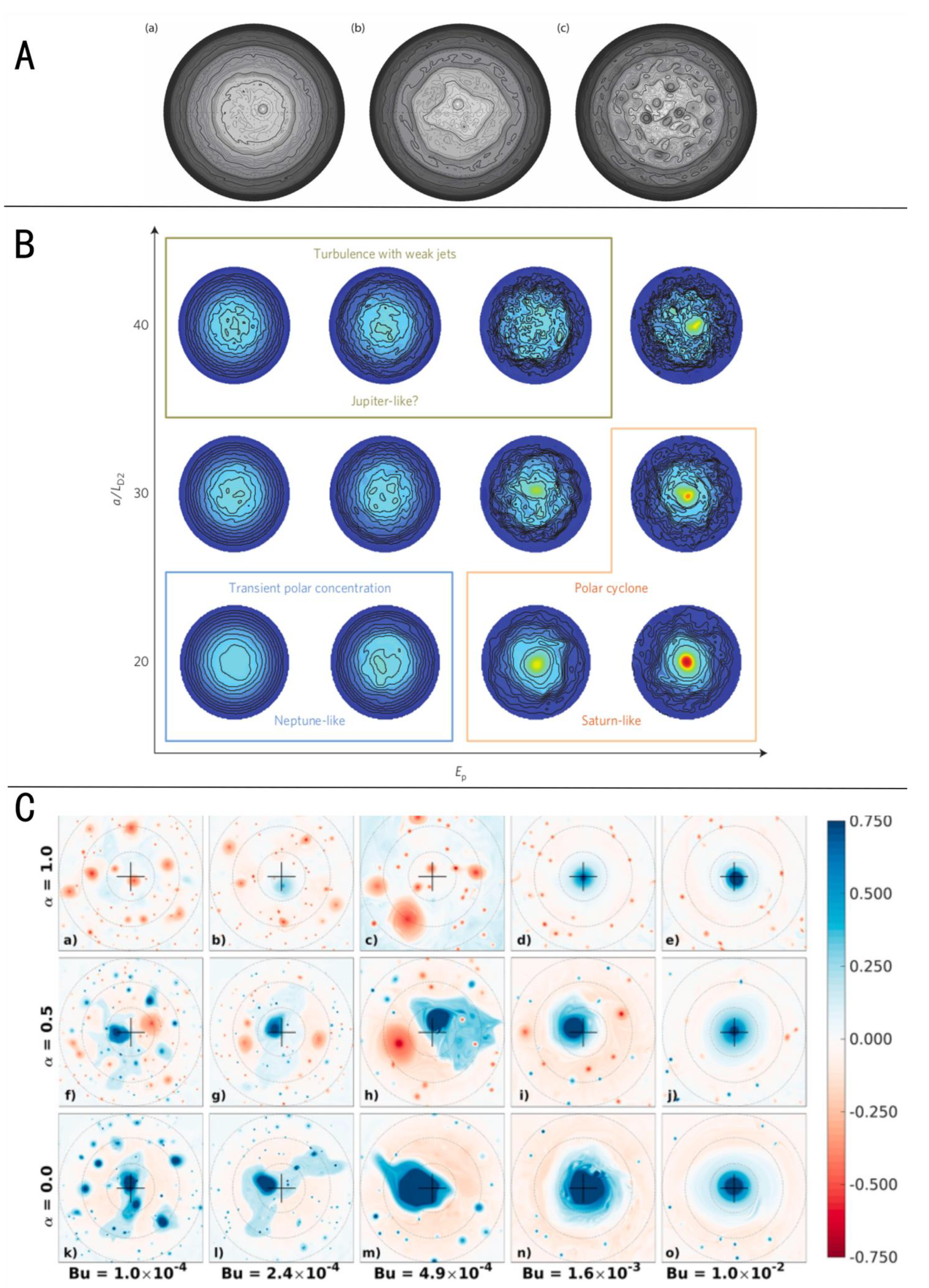
Observations and numerical simulations of atmospheres and oceans demonstrate that large-scale structures (e.g., jets and large vortices) spontaneously form from small-scale turbulence from the inverse-cascade effect of geostrophic turbulence [137]. Small-scale turbulence—on the order of a few dozen to a few hundred kilometers on giant planets—may be produced by cumulus convection and is widely thought to be a leading candidate source of momentum into zonal jets and large vortices, although other hydrodynamic instabilities are also involved (e.g., [14,125,138,139]). Theoretical studies (e.g., [140,141,142]), suggest that turbulent forcing in the polar regions should promote large-scale vortices rather than zonal jets, matching observations.

Here, we discuss how small-scale turbulence formed by cumulus convection aids in the formation and maintenance of jets and vortices. In Section 4.1, we will discuss cumulus convection and its source of small-scale turbulence. In Section 4.2, we focus on how turbulence self-organizes into zonal jets and discuss these results for the equatorial and mid-latitudes, using turbulent power spectra analyses and results from numerical modeling. In Section 4.3, we discuss how turbulence self-organizes into a largely vortex-dominated regime in the high latitudes, using numerical modeling and the results from power spectra analysis.

4.1. Turbulence and the Inverse-Cascade: Jets

Turbulence is ubiquitous in planetary atmospheres, and is generated by many processes, including cumulus convection. No one definition of turbulence seems to capture the entirety of this phenomena, however, we paraphrase [137]’s definition for our purposes: “turbulence is a large Reynolds flow dominated by non-linear effects and containing both spatial and temporal disorder with energy transferring at many different scales”. Observational, experimental, and numerical approaches with a variety of models and assumptions have all contributed to our understanding, however incomplete, of this branch of physics.

4.1.1. Turbulence: A Short Background for 3D, 2D, and Geostrophic Flows

Analyzing the dynamics of a turbulent fluid by constructing a spectral decomposition or structure functions (e.g., [143]) of a signal can provide clues to the processes shaping an atmosphere or ocean, including what mechanisms and at what scales energy is being injected into the atmosphere. Signals used in planetary atmospheric work are velocities derived from 1D and 2D cloud feature tracking to produce kinetic energy spectra, and another is from the reflectivity structure of clouds to produce a passive tracer spectra.

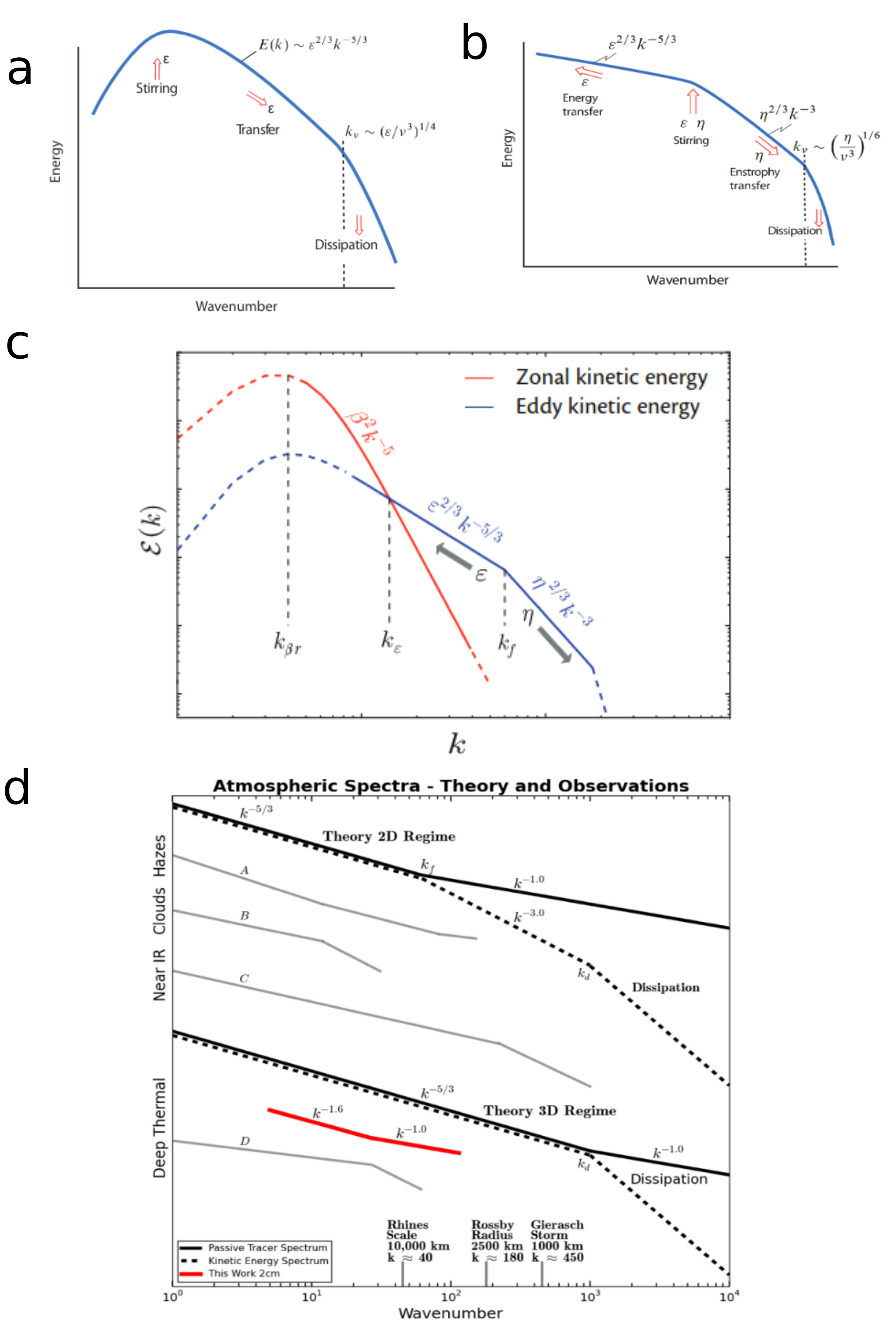
Conceptually, energy is added to a fluid at a scale or wavenumber, $k_f$, by convection or other hydrodynamic instabilities. In 3D turbulent motion, energy transfers to larger wavenumbers (smaller length scales) in a direct-cascade eventually to be dissipated at very small scales, $k_{\nu }$, by molecular viscosity. The essence of 3D turbulence is summarized by a rhyme familiar to fluid dynamists, “Big whorls have little whorls which feed on their velocity, and little whorls have lesser whorls and so on to viscosity” [144]. Figure 12a presents an idealized schematic of the 3D turbulent kinetic energy power spectrum, $\epsilon \left(k\right)$ as a function of wavenumber, k, with its characteristic $k^{-5/3}$ power dependence in the inertial range.

When 3D fluid flow is primarily constricted into quasi-2D flow as it largely is in the weather-layer of giant planet atmosphere, we see two fundamentally different behaviors. First, the energy preferentially transfers to smaller wavenumber, termed an inverse-cascade; small-scale motion is transferred into larger coherent structures, i.e., in Richardson’s parlance, small whorls build big whorls, see also [145]. However, the inverse-cascade appears to be somewhat scale-dependent; energy at small enough length scales preferentially proceeds in a direct cascade, see [139,146]. Such a situation may favor MCC-sized and larger convective disturbances in feeding energy into jets rather than from smaller convective storms, at least in the jet-dominated regions of the planet. Like 3D turbulence, the inertial range is characterized by a $k^{-5/3}$ power dependence. Second, enstrophy (mean square of the vorticity) preferentially cascades downscale to the dissipation scale, $k_{\nu }$, featuring a $k^{-3}$ power dependence, adding another inertial range to the power spectra for 2D turbulence (Figure 12d).

Charney’s geostrophic turbulence theory [147] describes idealized quasi-2D motion but did not consider differential rotation and boundary effects, which are key processes in real planetary atmospheres. Nevertheless, his theory has provided powerful insight into atmospheric dynamics. One such characteristic concerns kinetic energy spectra. He predicted a $k^{-3}$ slope should exist at the synoptic scale, shown as the dotted line in the top center of Figure 12d (1000–3000 km in Earth’s atmosphere). Measurements of terrestrial kinetic energy spectra clearly reveal the predicted $k^{-3}$ slope associated with energy transfer upscale and enstrophy transfer downscale. However, a $k^{-5/3}$ slope also exists at smaller scales (10–500 km in Earth’s atmosphere); located in the “dissipation region” of Figure 12d) with different interpretations attempting to explain it (e.g., [148]). However, models using the surface quasigeostrophic theory, (SQG), e.g., [149,150,151] show that a $-5/3$ slope is expected at high wavenumbers.

The presence of differential rotation or $\beta$, the planetary vorticity gradient, and stratification are critical factors in the formation of zonal jets. These factors are widely studied in rotating tanks and a variety of numerical experiments using different models, e.g., [142,152,153,154,155,156,157,158]. A familiar outcome of these experiments is the formation of zonal jets with a characteristic meridional width (see Figure 12a and Figure 13a). Rhines [140] made a significant breakthrough in quasi-2D theory with differential rotation by investigating flow where large-scale atmospheric wave motion, such as Rossby waves, interact with smaller-scale isotropic turbulent motion. Rossby waves arise from the conservation of potential vorticity, $q=\frac{f+\zeta }{h}$ where f is the planetary vorticity, $\zeta$ is the vertical component of relative vorticity and h is a measure of fluid thickness. The gradient of f, i.e., $\beta$, acts as a restoring force. Small-scale isotropic turbulent motion is initially too small to be affected by $\beta$ and such flow is dominated by eddies rather than waves. However, in differential rotation with low friction these eddies grow in size via the inverse-cascade. At the Rhines length, $L_R={\left(\frac{U}{\beta }\right)}^{\frac{1}{2}}$, where U is a characteristic velocity scale, turbulent eddies feel the influence of $\beta$, deforming anisotropically into planet-encircling east-west jets (termed zonation) with a limited meridional width, this width scaling favorable with $L_R$, e.g., [16,159] for an alternatives behind jet formation that do not involve turbulent energy cascades).

Figure 12. Idealized Turbulent Energy Power and Passive Tracer Power Spectra. (a) Idealized 3D Turbulent Energy, (b) Idealized 2D Turbulent Energy, (c) Idealized Geostrophic Energy. (d) Turbulent Energy vs. Passive Tracer Spectra. (a–c) Reproduced from [137] (d). Select Jupiter spectra reproduced from [160]. Thin black lines labeled A–D and the thick red line are for individual observations detailed in [160].

Figure 12. Idealized Turbulent Energy Power and Passive Tracer Power Spectra. (a) Idealized 3D Turbulent Energy, (b) Idealized 2D Turbulent Energy, (c) Idealized Geostrophic Energy. (d) Turbulent Energy vs. Passive Tracer Spectra. (a–c) Reproduced from [137] (d). Select Jupiter spectra reproduced from [160]. Thin black lines labeled A–D and the thick red line are for individual observations detailed in [160].

The presence of rapid rotation and $\beta$ profoundly changes the nature of 2D turbulence, schematically shown in Figure 12a. Here, an additional inertial regime, called zonostrophic [161] is often found, featuring a $k^{-5}$ power dependence along the zonal direction of motion (red curve) and a $k^{-5/3}$ along the meridional direction of motion. Figure 12d shows a comparison of kinetic energy and passive tracer power spectra, along with plots from observations of Jupiter at optical, 5 $\mathsf{\mu }$m infrared, and 2 cm radio wavelengths, which probe at different levels of the atmosphere. Note, kinetic energy and passive tracers have differing wavenumber power-dependence (e.g., [137,162,163] and references therein). Here too, at smaller scales than shown in Figure 12c, a −5/3 slope is often encountered as previously described.

4.1.2. Retrieved Kinetic Energy Power Spectra from Giant Planet Atmospheres

Mitchell [164] and Mitchell and Maxworthy [165] investigated the kinetic energy power spectra of Jupiter using Voyager 1 and 2 image sequences of the zonal-averaged motion of the cloud tops (P∼700 mb), finding a $k^{-5/3}$ power-dependence in line with geostrophic theory. Later, Galperin et al. [166], found evidence of a zonostrophic $k^{-5}$ spectrum for zonal flows on Jupiter and Saturn. Observations taken from the Cassini flyby of Jupiter and using an automated cloud feature tracking clearly showed small-scale eddies feeding momentum into the zonal jets [167], confirming the findings of Beebe et al. [168]’s manual cloud tracking using Voyager 2 observations of Jupiter. Del Genio et al. [65] found similar eddy-to-jet momentum transfer from Cassini observations of Saturn. Choi and Showman [169], using Cassini and HST data sets and 2D automatic cloud tracking of Jupiter’s cloud tops for both kinetic energy and passive tracer spectra found evidence of geostrophic turbulence, but with slopes transitioning at different high wavenumbers, 70 vs. 200 for kinetic energy and passive tracer, respectively. In both spectra, however, the forcing scale appeared to be close to that of the Rossby deformation radius, $L_D$, which suggests baroclinic instability is involved. However, baroclinic instability and cumulus convection, particularly in MCCs, may not be mutually exclusive because baroclinic instability may help trigger convective outbreaks on giant planets, as it does on Earth, and can occur on similar length scales, e.g., [12,125].

Young and Read [139] also retrieved energy power spectra from Cassini flyby data of Jupiter finding spectra and cascades with some features characteristic of geostrophic turbulence, but also found some features distinctly inconsistent with geostrophic turbulence theory. A $k^{-5/3}$ slope for k > 80 (5000 km and smaller) was retrieved but, strangely, at small wavenumbers, the spectra flattened, which they expressed as “distinctly non-terrestrial”. Furthermore, they did not report an expected zonostrophic $k^{-5}$ slope. They found evidence of an inverse-cascade of energy from $L_D\sim 2500$ km, upwards to the meridional jet width ∼9000 km (expected from geostrophic theory) but also found a forward cascade of energy from very large scales ∼ 40,000 km to the meridional jet width, which was unexpected. Clearly, energy was observed being pumped into the jets from both small and larger scales. A forward enstrophy flux was found from the jet width to the smallest scales observed—consistent with geostrophic theory—but they found no inertial range, which is inconsistent with geostrophic theory, but may be indicative of frontogenesis processes and filamentary formation. They suggest that because the crossover length between upscale and downscale energy transfer appears around $L_D$, baroclinic instability may be the energy injection mechanism instead of convection. Young and Read [139] were careful to note that baroclinic instability on giant planets may be concentrated near the tropopause, biasing the cloud-top derived data, and, if so, SQG theory may be more applicable to explain some of their results, which predicts an energy reversal around $L_D$. It is important to point out that MCC cumulus convection easily can reach the expected scale of $L_D$. Furthermore, if frontogenesis processes are operating, it may aid the development of cumulus convection if these fronts are discontinuities in humidity or temperature, or if gravity waves are generated, because these effects can become efficient mechanical and thermal triggers to initiate lifting of moist air, as is the case on Earth.

4.1.3. Retrieved Passive Tracer Power Spectra from Giant Planet Atmospheres

Harrington et al. [170] used passive tracer power spectra taken at 5 $\mathsf{\mu }$m, probing ∼1–5 bar pressure depth, providing evidence for an inverse-cascade, and suggested that baroclinic instability may be a significant process for energy injection at these depths. Barrado-Izagirre et al. [171] used both HST and Cassini flyby data of Jupiter’s cloud tops, finding that the power spectra is consistent with geostrophic turbulence. They estimate the energy forcing occurs around 1000 km, again consistent with baroclinic or MCC-sized convective instability. Cosentino et al. [172] used passive tracer spectra derived from VLA (Very Large Array) observations at a wavelength of 2 cm, which probed Jupiter at and beneath the cloud tops at ∼0.5–2 bar showing strong evidence that geostrophic turbulence largely governs these pressure levels in the atmosphere, and found a wavenumber associated with the spectral transition of the slopes to be ∼13,000 km, a value close to the Rhines scale at the equator and similar to that of Harrington et al. [170]. This size may be in line with a trapped equatorial Rossby wave thought to be the dynamical mechanism behind the plumes and 5 $\mathsf{\mu }$m hot spots of the North Equatorial Belt (NEB). Continuing with a similar approach, Cosentino et al. [163] probed Jupiter’s visible cloud decks using a passive tracer power spectrum derived from HST data. Interestingly, they found differences in the power spectra slopes between the cyclonic belts and anticyclonic zones. Perhaps more relevant to this paper, they found that in some latitudinal bands a forcing scale wavenumber ($k_f$) as high as 100–400 may exist, which could correspond to a size of convective storms. Cosentino et al. (2019) found that at low wavenumbers (k < 20), the spectral slope was rather flat, which is somewhat in line with the findings of Sukoriansky et al. [154] for zonostrophic flow with large-scale drag or friction. What causes this drag was not specified, but large-scale drag is expected to exist.

The key take-away from the kinetic energy and passive tracer spectra investigations referenced above strongly suggest that geostrophic turbulence largely governs flow in the weather layer of the giant planets, albeit with some important deviations, supporting baroclinic or convective storms as an energy source.

4.2. Numerical Modeling of Jet Dynamics on Giant Planets: Forcing and Organization

Two broad paradigms exist regarding the formation and maintenance of zonal jets. The first is “deep-forcing”, which posits that zonal jets are a surface manifestation of differential rotation acting on dry convection deep in the interior, sometimes termed flow on cylinders. The second is “shallow-forcing”, which posits that cumulus convection and baroclinic instability, acting in the weather layer, form and maintain zonal jets (and large vortices) via geostrophic turbulence, and can barotropize these jets well below the depth where forcing occurs (e.g., [16,158,159,173] for reviews). It is possible that both are involved but perhaps one dominates in different latitudinal regions than the other. Given the lack of frequent in-situ data from the giant planets, employing numerical modeling is necessary to explain atmospheric observations of the giant planets and resolve which forcing mechanisms are primarily responsible for powering the jets. General references discussing the application and fundamentals of atmosphere modeling are numerous and beyond the scope of this paper (see, e.g., [137,174,175,176,177,178,179,180,181,182]). One key difference regarding relevant giant planet atmospheric models worth mentioning regards the nature of the forcing. Some models are seeded with turbulence in their initial conditions but otherwise are left to freely evolve, termed freely-decaying. Others are continuously or periodically forced with turbulence, often applied in discrete random patches, which can simulate more realistic temporal processes in the atmosphere, termed forced-turbulent.

Early models using freely-decaying turbulence, e.g., [141,183,184] demonstrated that jet formation spontaneous emerges on a rotating sphere with steep potential vorticity (PV) gradients (jets) separating more homogenized bands between at least in some cases, depending on the model and tuning of specific parameters such as rotation rate and $L_D$, see [185]. The initial turbulence applied was not particularly geared towards simulating cumulus convection, however. A more recent freely-decaying model solving the more sophisticated primitive equations was provided by [186]. Their results demonstrated that zonal jets are a typical result from the inverse-cascade, that barotropic jets can emerge without barotropic forcing, and that anisotropic turbulence emerges when $L_D$ > $L_R$, consistent with results of Cho and Polvani [141], Okuno and Masuda [142], Theiss [187], and Showman [155]. Freely-decaying models have also been applied to study giant planet convection focusing on specific jets or detailed dynamics and/or morphology of a thunderstorm clouds (e.g., Hueso and Sánchez-Lavega [135], Hueso [138], Sánchez-Lavega et al. [22], to cite a few examples).

Forced-turbulent models that attempted to include some convective processes include those of Li et al. [188], Showman [155], Scott and Polvani [189], and Cosentino et al. [190]. Showman [155] applied moist convection of scales similar to cumulus MCCs, mimicking their effect on the atmosphere by using mass pulsing. All of these models were able to replicate more observed features of jets and vortices than the previously mentioned freely-decaying studies. Results of these models included: convection driving the zonal jets on Jupiter and Saturn; PV staircases emerged; long-lived anticyclonic vortices analogous to Jupiter’s GRS emerged; a vortex-dominated regime tends to dominate in the polar regions with jets dominating elsewhere. These models also tested the role of energy forcing, damping, rotation rate, and $L_D$ on the strength and width on the resulting jets. However, while showing that moist convection is important for jet formation and maintenance, the motion of the equatorial jet was often in the wrong direction.

Additional insight into the mechanism of giant planet jet formation and maintenance was found in Liu and Schneider [159], Liu and Schneider [191], and Liu and Schneider [192]’s studies using a primitive equations model. Forcing was conducted applying a constant heat flux at the bottom of the domain simulating a planet’s intrinsic heat flux. They found that the off-equatorial jets are formed and energized by baroclinic eddies. Rossby wave generation in the equatorial region, created by dry-convection below the weather layer, is responsible for the formation of prograde equatorial jets. Their results suggest that retrograde equatorial jets on the ice giants are probably a result of insufficient heat flux from the interior (Uranus) or too strong of baroclinic forcing in the non-equatorial region (Neptune). The dry-convection scheme used in these three studies does not apply to cumulus convection but, because the model’s lower boundary was at only ∼3 bar, some of the results found are suggestive that cumulus convection, which occurs in the weather layer might have similar results.

Lian and Showman [193], using a primitive equations model with water latent heat effects added into the energy equation, were able to reproduce the prograde (Jupiter and Saturn) and retrograde (Uranus and Neptune) equatorial jets in a single model, testing the effect of planetary rotation, radius, gravity, and deep-water abundance. Cumulus convection was not explored in a manner similar to Showman [155]. However, the effects of latent heat release by water profoundly effected the results, favorably matching observations of the giant planets. They found that high water abundance tends to form retrograde equatorial jets, whereas moderate water abundance tends to form prograde equatorial jets. Similar to previous studies, Lian and Showman [193] found that the release of latent heat from water generated baroclinic eddies, which, in turn, interacted with the large-scale flow pumping momentum into the zonal jets. However, as noted in Lian and Showman [194], baroclinic instabilities can pump momentum into the jets from the cyclonic or anticyclonic side of a jet. Cumulus convection, on the other hand, would tend to apply the momentum from the cyclonic flank only. Lian and Showman [193]. Both studies, however, acknowledged, that MCC-scale cumulus convection would need to be a focus of a future study to determine how such forcing would compare to the large-scale baroclinic eddy production in models capturing the effect of water latent heat release.

Clearly, the results of the few studies summarized in this section demonstrate that moist convection from water appears to be a necessary ingredient in modeling and explaining the observations of jet formation, maintenance, strength, and flow direction on the giant planets. Considering that cumulus convection is likely to be a considerable energy source into the atmosphere, is observed more frequently in the cyclonic belt regions, and may be intimately intertwined with baroclinic processes, its role in jet dynamics on the giant planets will continue to be investigated for the foreseeable future.

4.3. Turbulence and the Inverse-Cascade: Vortices

4.3.1. Large Vortices on the Giant Planets

The gas giants feature numerous vortices of different sizes and lifespans. The midlatitudes contain a large number of anticyclones, e.g., [195], including Jupiter’s GRS and Oval BA, the largest two anticyclones on the planet (see Figure 13a). The GRS has existed for at least 150 years, perhaps longer. There are no observations showing formation of GRS, so we cannot say if cumulus convection was involved. Unlike the GRS, the formation of Ovals BC, DE, FA in 1939–1940 was observed, which merged to form Oval BA in 2000, and has drawn comparisons to large-scale disturbances in Jupiter’s belts and zones [196]. These large-scale disturbances might have their origin in convective storm outbreaks.

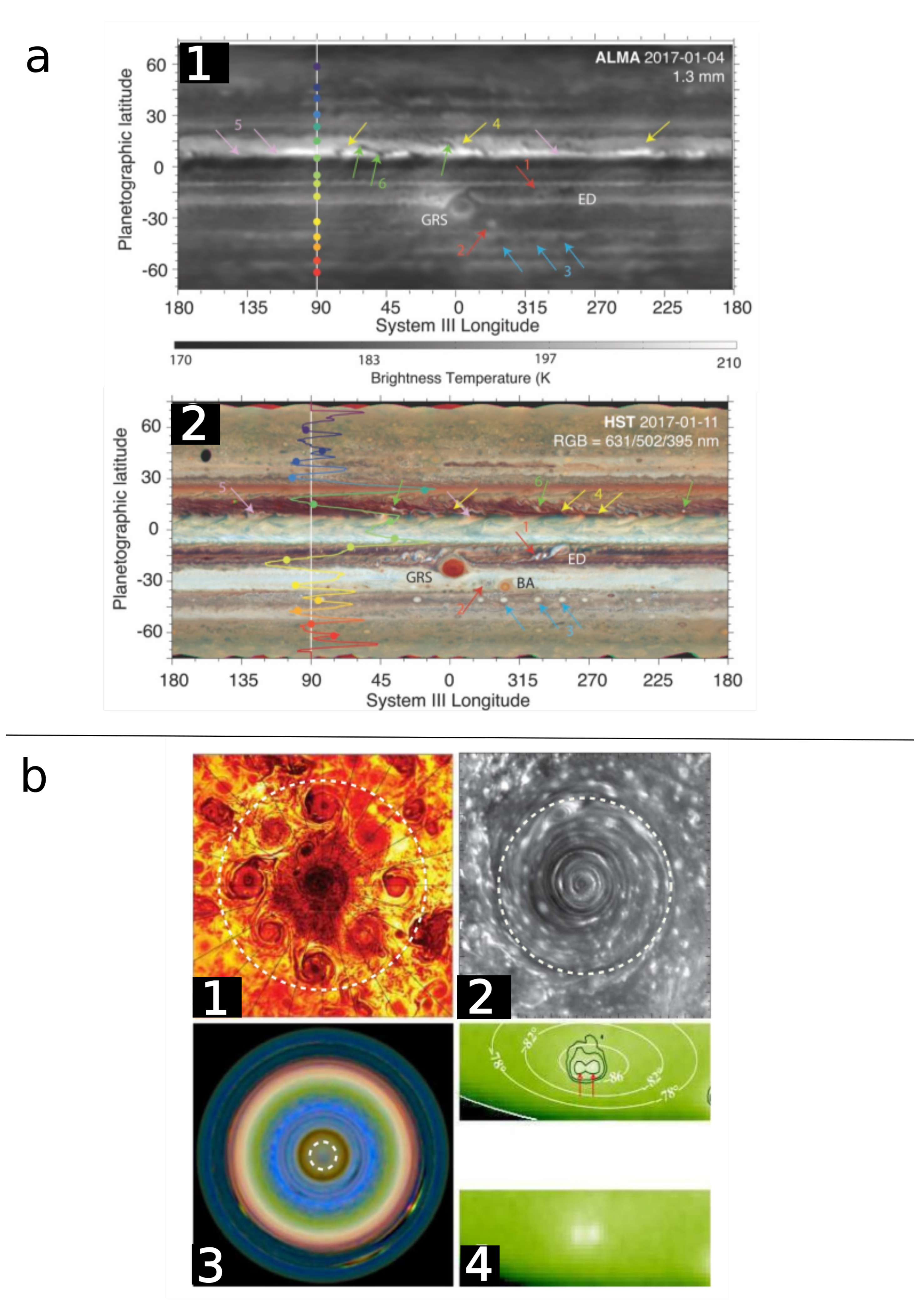
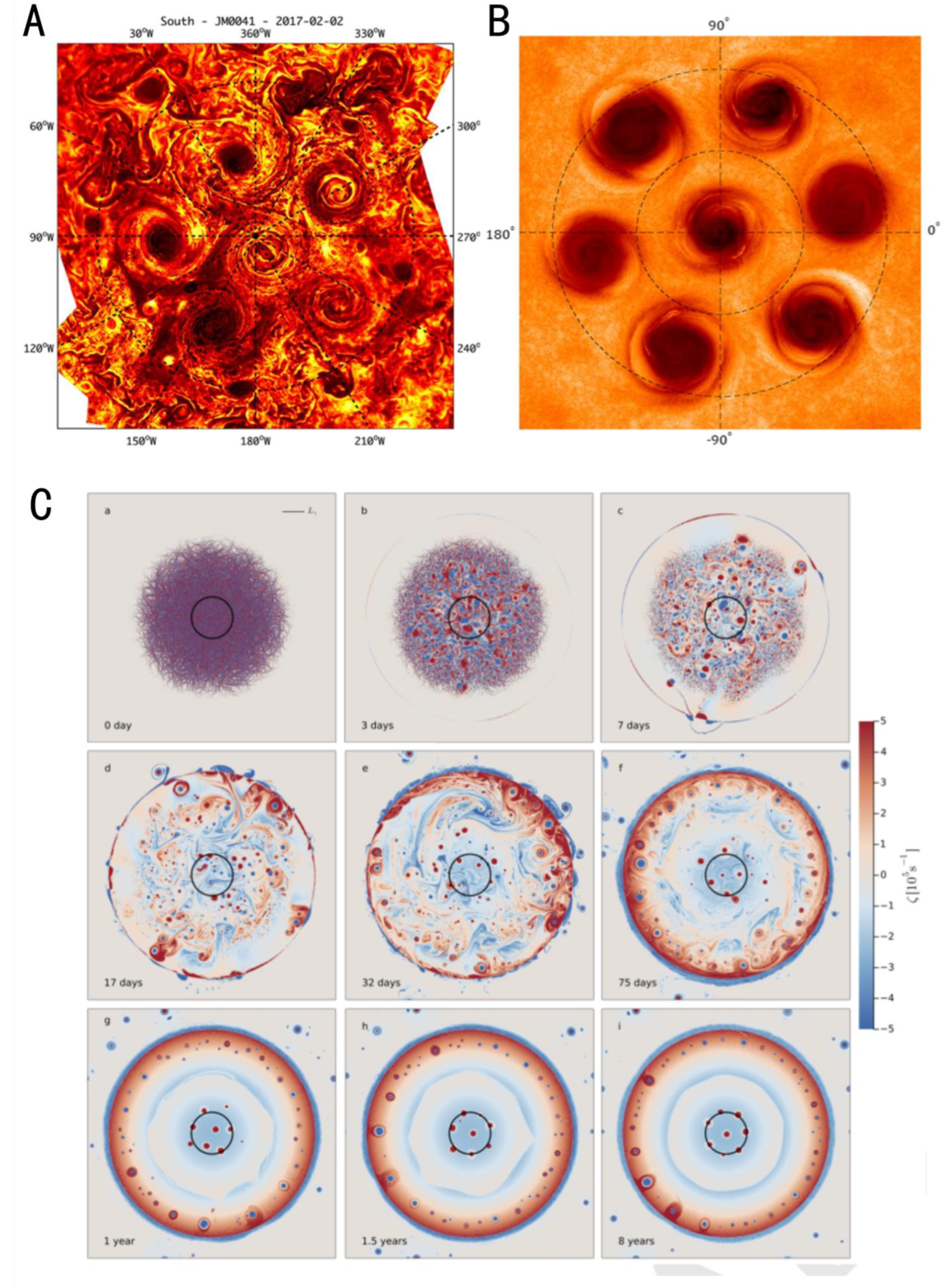
Jupiter’s polar regions feature large long-living cyclones featuring a slightly off-set polar cyclone surrounded by a ring of close-packed circumpolar (CPC); 8 in the north, and 5–6 in the south (see Figure 13b). The existence of such close-packed cyclones on Jupiter has presented a challenge to our understanding of atmospheric dynamics as vortices with the same polarity are expected to merge when in close proximity. Cumulus convection has been frequently observed in the polar regions. A shallow ($\mathrm{P}<2 \mathrm{bar}$) lightning flash was detected by JunoCam in the outer part of a CPC with a morphology suggestive of cumulus convection during the 31st perijove. Additional evidence is provided by lightning statistics derived from the Microwave Radiometer (MWR, [197]) showing that the polar regions contain abundant cumulonimbus convection [17]. JunoCam and JIRAM also reveal that a few anticyclones exist near and just equatorward of the rings of CPCs. The mechanisms that sustain these cyclonic configurations without merging are a subject of considerable research at present. Furthermore, much like jet dynamics, the role of shallow vs. deep forcing to explain polar cyclone dynamics remains unresolved. As Juno’s periapse moves to higher northern latitudes during the Extended Mission, MWR is expected to reveal critical depth-dependant dynamics, which may address the role of forcing depth. Continuing equatorward, a broad region on Jupiter exists where the FFRs are common place and where cumulus convection, evident from lightning flash data from MWR, is frequently observed. Still further equatorward, the familiar banded jet-dominated structure previously discussed becomes apparent with anticyclones generally found within the anticyclonically sheared zones and with cyclones generally found within the cyclonically sheared belts. Cumulus convection and lightning flashes are more frequently found in the belts than in the zones [16].

Figure 13. Banded Structure of Jupiter and Polar Cyclones. (a1) 1.3 mm Radio Map of Jupiter. (a2) RBG HST Image of Jupiter showing zonal wind direction as a function of latitude and various features. a. Reproduced from de Pater et al. [198] (b1) Jupiter. (b2) Saturn, close−up of North Polar Cyclone. (b3) Uranus. (b4) Neptune. Figure reproduced from Brueshaber et al. [199] and references therein.

Figure 13. Banded Structure of Jupiter and Polar Cyclones. (a1) 1.3 mm Radio Map of Jupiter. (a2) RBG HST Image of Jupiter showing zonal wind direction as a function of latitude and various features. a. Reproduced from de Pater et al. [198] (b1) Jupiter. (b2) Saturn, close−up of North Polar Cyclone. (b3) Uranus. (b4) Neptune. Figure reproduced from Brueshaber et al. [199] and references therein.

Saturn generally follows the same latitudinal description as Jupiter with a few exceptions. One, the polar regions feature a solitary pole-centered cyclone instead of a central off-set cyclone surrounded by a ring of CPCs (see Figure 13b). Two, while clouds suggestive of cumulus morphology exist in the polar regions, lightning has not been definitively detected, which might suggest strong H${}_2$O-based cumulus convection is not a major force in forming or maintaining the polar cyclones (see too the subsection on polar numerical modeling below). Three, FFRs do not seem to be a common feature on Saturn. Four, the belt-zone jet configuration on Saturn is similar to Jupiter, but appears to extend to higher latitudes, and does not contain a GRS-like anticyclone. Five, cumulus convection tends to be less frequent on Saturn overall but, at times, can be very powerful and cumulus convection originating in the H${}_2$O-cloud is the mechanism behind the apparition of the roughly 30-year cycle Great White Spot outbreaks, e.g., [52]. These GWS outbreaks appear to be large MCCs and the active convective period lasts for months. The MCCs shed a turbulent wake from which relatively cloud-free anticyclones form. The most recent GWS outbreak also formed the largest anticyclone observed to date in the Solar System, interestingly, in the stratosphere rather than in the troposphere [200].

The ice giants, like Saturn, appear to feature large solitary pole-centered cyclones, although wind measurements are challenge to obtain (e.g., [68] see also Figure 13b). High-altitude thick and seasonally-varying hazes combined with long orbital periods and infrequent observations (particularly by spacecraft) greatly impact our observations of the polar regions on these planets. It is difficult to determine if such polar cyclones exist year-round as on Jupiter and Saturn, or come and go seasonally as in Earth’s stratosphere. Curiously, not long after the most recent solitice on Uranus, observations from earth revealed large cumulus-appearing clouds similar to those seen on Saturn, but much larger, e.g., [201]. Interestingly, cyclones are noticeably absent outside the polar regions. Large anticyclones are present outside the polar regions but are fewer in number than on the gas giants, those that do appear from time to time present as dark anticyclonic spots (probably as a result of thinning of the H₂S clouds at P > 4 bar), often sporting white methane ice companion clouds. It is unknown what mechanisms are responsible for the lack of cyclones and the infrequent appearance of the dark anticyclones. We have no direct evidence to date from the ice giants that small-scale turbulence organizes into dark anticyclones, and these could result from deeper-seated baroclinic or barotropic instabilities shedding a large vortex, which then either rises or barotropizes a thick section of atmosphere to become visible to Earth- and space-based telescopes. Determining the formative mechanism(s) behind these large anticyclones on the ice giants probably demands an orbiting spacecraft.

As previously noted, turbulence can self-organize into larger-scale vortices as well as jets. Different mechanisms have been invoked to explain the origin and maintenance of long-lived vortices on the giant planets. Barotropic, baroclinic, and convective instabilities have all been shown to be able to create vortices in the laboratory and in numerical studies. However, the organization of small-scale turbulence into large features via geostrophic turbulence shows that the gradient of the Coriolis force, which is a function of latitude (i.e., $\beta$), has an strong effect in determining if jets or vortices are favored. Okuno and Masuda [142] and Smith [202], extended Rhines’ work on jets to include a finite deformation radius $L_d$ (barotropic theory assumes $L_d=\infty$) and found that the Rhines length is modified to take the form

$$\begin{array}{c}\hfill L_R^{\prime }={\left(1/L_R^2-1/L_{\mathrm{d}}^2\right)}^{-1/2.}\end{array}$$

(3)

In this modified form, $L_R^{\prime }$ becomes imaginary when $L_d<L_R$ and turbulent self-organization leads to vortex-dominated flow rather than jet dominated flow. Theiss [187] demonstrated that the degree of anisotropy weakens as a function of increasing latitude and showed that a critical latitude exists above which the pattern of alternating zonal flow breaks down to form a regime consisting of coherent vortices, which was numerically confirmed with the results of Showman [155]’s and Sayanagi et al. [186]’s (among others) modeling of jet dynamics. Note, this transition from jet- to vortex-dominated regions as a function of latitude clearly does not preclude the existence of long-lived vortices equatorward of a critical latitude (e.g., Jupiter’s Great Red Spot).

4.3.2. Power Spectra in Giant Planet Large Vortices

In this section, we discuss power spectra and forcing mechanisms that have been applied to the formation and maintenance of vortices on the giant planets.

The spectacular views from both JIRAM and JunoCam of Jupiter’s poles and high latitudes have drawn visual and dynamical comparisons to eddies in Earth’s oceans. Few turbulent power spectra analyses have been completed for the polar regions on the giant planets; we are aware of only Jupiter being subjected to such analyses in the polar regions. Here, we present results prior to and during the Juno epoch to shed light on the dynamics of polar cyclones as revealed by power spectra analysis.

Prior to Juno, many numerical experiments seeking kinetic power spectra studied rapidly rotating turbulence with 3D forcing. Here, we mention a few as they provide context to power spectra retrievals from the Juno observations. Smith and Waleffe [203] used a 3D forced-turbulent model with an f-plane approximation, which mimics the near-constant value of f near the pole. Their results showed the expected $k^{-3}$ and $k^{-5/3}$ power slopes consistent with Charney’s geostrophic turbulence theory. Furthermore, they found that most of the energy at $k<k_f$ was contained in 2D structures, which they claimed to be analogous to the process of zonation in jet dynamics. Such an effect, like that in the jet-dominated regions, suggests that small-scale activity such as moist convection and baroclinic instabilities may form and maintain the polar cyclones on the giant planets (see also the following subsection).

Motivated by the unexplained $k^{-5/3}$ energy power spectra slope at mesoscale lengths (often defined as ∼ 2–2000 km; Orlanski [204]) found in terrestrial tropospheric measurements [205], Tulloch and Smith [150] applied a variation of surface-quasigeostrophic (SQG) models to the problem. Focusing on the transition between quasi-2D barotropic and 3D baroclinic flows, their finite-SQG model power spectra results showed the expected $k^{-3}$ slope at $k=k_f$, with a slightly greater slope at $k<k_f$, which is consistent with 2D forcing with drag. Additionally, they found a $k^{-5/3}$ slope at $k>k_f$, roughly matching the tropospheric measurements, showing, among other studies, that SQG can be applicable in a planetary atmosphere.

Rubio et al. [206] conducted numerical experiments with another useful category of models, i.e., rapidly rotating Rayleigh–Benard (RRRB) theory, where convection from thermal forcing stirs the fluid. They noted that large-scale barotropic vortices emerged, which, in turn, organized small-scale convective eddies. These eddies provided a “dynamically evolving energy source” for the large-scale barotropic flow. The barotropic kinetic energy spectra featured a $k^{-3}$ slope from very small wavenumbers to large wavenumbers $k>k_f$. The small-scale baroclinic eddies featured a $k^{-5/3}$ slope in a more narrow wavenumber range and steepening to an unspecified slope at $k>k_f$. These results suggest, but do not explicitly show, that cumulus convection could be involved in shaping the structure of Jupiter’s polar cyclones.

After Juno’s orbit insertion on 4 July 2016, imagery acquired from JIRAM’s M-filter (∼4.9 $\mathsf{\mu }$m) has been used to retrieve both energy and passive tracer spectra of Jupiter’s polar region. To our knowledge, we are aware of only three studies that have published on such spectra from a giant planet’s atmosphere. Noting a striking resemblance of Jupiter’s turbulent polar clouds to turbulent features in Earth’s upper ocean buoyancy profiles and potential temperature structures near the troposphere, including fine filamentary structures, some researchers noted that SQG theory might be applicable to explain polar dynamics. Adriani et al. [207] conducted an energy power spectra analysis for one CPC at the south polar region and found that their power spectra retrieval bore a strong match to SQG theory and simulations. These results suggest that small-scale dynamics (much smaller than the CPCs) such as filaments and frontal zones control mixing. Frontal zones are sharp gradients of a scalar such as temperature and humidity, and may be critical to triggering cumulus convection. Frontal zones exhibit large vertical velocities and are clearly correlated with, and provide a lifting mechanism to, initiate both small-scale ($\mathcal{O}($10) km) and MCC-scale convection ($\mathcal{O}$ 100–1000 km) on Earth where fronts are commonly found in baroclinically unstable regions (e.g., midlatitudes).

Moriconi et al. [208] conducted a more thorough, passive-tracer, retrieval analysis to the region at and poleward of the ring of Jupiter’s southern CPCs, and to the region just equatorward of the ring of CPCs. Their results showed a power-spectra best fitted with two slopes—consistent with an idealized 2D turbulence theory—with the kink in the slope occurring at ∼500 km, which they attribute to being the size of $L_D$. While this value for $L_D$ is a reasonable estimate for Jupiter’s poles, their retrieved slopes deviate from predictions from theory. At length scales $>L_D$, their power spectra featured $k^{-1}$ slopes, but a $k^{-5/3}$ slope is expected from a quasi-2D passive tracer. At length scales $<L_D$, they retrieved a slope of ∼$k^{-3.3}$. This value is reasonably consistent with quasi-2D energy spectra, not a passive tracer spectra (see Figure 12d). It is not entirely clear what mechanisms are responsible for the deviation from quasi-2D theory but suggest that dynamics not related to the circulation of the CPCs may be involved, including temperature and pressure gradients.

Ingersoll et al. [209] used JIRAM’s M-filter images of the north polar region acquired during Juno’s 4th periapse searching for signals of convection by analyzing the correlation between divergence and vorticity. They found no correlation between these variables. They note that if a convectively unstable parcel ’resets’ its vorticity to zero at the start of the updraft, then negative vorticity develops on rising trajectories and the parcel diverges at the top leading to a correlation between divergence and vorticity. If, on the other hand, the parcel conserves potential vorticity around a cycle of updrafts and downdrafts, then a measurable correlation is not expected. However, the feature-tracking method applied by Ingersoll et al. [209] was only reliable at scales of ∼200 km and greater.

To analyze smaller scales, Siegelman et al. [210] used the same data set as Ingersoll et al. [209] with an alternative approach. By correlating JIRAM image brightness to cloud height, they are sensitive to scales far smaller than Ingersoll et al. [209]’s method (∼15 km vs. ∼200 km). Large optical depth values are associated with the signature of updrafts, which condense clouds and block the transport of heat from Jupiter’s interior making these regions appear dark in the M-filter Adriani et al. [211]. The opposite is true for downdrafts, which evaporate cloud condensates allowing for more heat transport through the upper troposphere to space, making these regions appear bright. In the SQG-framework applied here, optical brightnesses are a proxy for a vertical scale and then can be related to available potential energy (APE) (e.g., [212] for applications to Earth’s tropopause). Simple relations between horizontal motions and a vertical scale are a feature of SQG theory. Images at 10 km/pixel resolution exhibited intermediate-scale (500–1600 km) vortices and small-scale filaments (100 km) associated with the large-scale vortices (5000 km). 2D wind velocities and optical depths were retrieved from this data set. Additionally, the optical depth can be used to diagnose the relative vorticity. Putting these concepts together, Siegleman et al. (2022) found turbulent energy spectra with a $k^{-3}$ slope at scales larger than 1600 km and a $k^{-4/3}$ at smaller scales, which matches very favorably with RRRB-modelling. Additionally, they found an upscale transfer (inverse-cascade) of KE energy from cumulus-convection scales (100–500 km) upwards to the CPC-scale of 5000 km, and claim that moist convection is driving an upscale energy cascade. Their analysis of the magnitude of CAPE values retrieved, however, suggest NH${}_3$-layer based cloud convection, rather than the more powerful H${}_2$O-layer based cloud layer is responsible.

If cumulus convection is ultimately driving Jupiter’s CPCs, it remains to be determined if NH${}_3$-cloud convection—likely presenting as weaker, non-cumulonimbus forms—alone is energetic enough. However, Saturn’s long-duration polar cyclones feature fast winds. However, strong cumulus convection, as evident from lightning detection associated with H${}_2$O-based convection, appears to be absent there. Cumulonimbus clouds on Jupiter, whether alone or organized into MCCs, co-exist with other non-cumulonimbus cloud forms and given the very small scales reported by Siegelman et al. [210] that are transporting energy upscale, cumulus clouds at scales at or smaller than MCCs may be contributing energy to the CPCs.

The dynamics that have been invoked from various models (e.g., QG, SQG, RRRB) and from the retrieved power-spectra analysis support the hypothesis that clouds, temperature, and humidity gradients can be organized into narrow regions by large-scale flow, which may act as frontal zones. These fronts could trigger cumulus convection by providing a thermal or mechanical mechanism to lift moist air to the LFC. To date, we have only obtained power spectra retrievals for Jupiter’s polar cyclones and its largest and long-lasting mid-latitude anticyclones, the Great Red Spot and Oval BA. However, it is expected that the dynamics that form and maintain these anticyclonic vortices are likely to be relevant for Saturn, and may also hold some relevance for the ice giants.

4.3.3. Numerical Modeling of Polar Vortices on Giant Planets: Forcing and Organization

A key process affecting the dynamics of the vortex-dominated polar regions on rapidly rotating planets is beta-gyre drift, which is a non-linear phenomenon in which the rotation of a vortex advects the environmental PV gradient around itself, e.g., [213]. The environmental PV gradient is directly related to $\beta$, with larger values of $\beta$ creating a greater beta-gyre drift rate [214]. Due to the conservation of PV, secondary vortices called beta gyres form to the southwest and northeast of the primary vortex. The system of vortices drives a “ventilation wind” [215] over the primary vortex, steering cyclones poleward and westward, and anticyclones equatorward and westward. The result of beta-gyre drift is an accumulation of cyclonic vorticity towards the polar regions. Beta-gyre drift has been simulated in numerical models and has been observed for hurricanes in Earth’s atmosphere, Mediterranean Salt Lenses (Meddies) in the Atlantic Ocean, e.g., [216], and the Great Dark Spot on Neptune, e.g., [217].

Shallow-water simulations in the pre-Juno epoch, e.g., [141,155,189] numerically confirmed Rhines’ and Theiss’ results that a midlatitude jet-dominated regime transitions to a vortex-dominated polar regime. Scott and Polvani [189], using a forced-turbulent approach, found that planetary Burger number, $Bu={(L_D/a)}^2$ where a is the planetary radius, influences whether the inverse cascade forms jets or vortices, with vortices tending to emerge in the high latitudes and jets dominating elsewhere (see Figure 14A). Showman [155] used the Explicit Planetary Isentropic (EPIC [218]) model with a forced-turbulent approach to demonstrate how turbulence generated by parametrically simulating moist convective storms with mass pulses, which mimic the effect of mass being injected into a layer from below, will self-organize into jets at low latitudes, and a vortex-dominated regime at higher latitudes. Scott [219] tackled how the inverse-cascade affects the polar regions with a simple, 1-layer quasi-geostrophic (QG) model, and like Scott and Polvani [189] finds a variety of dynamical outcomes may emerge depending upon planetary radius and $L_D$. Instead of using mass pulses, they placed fully formed cyclonic and anticyclonic vortices into the domain in a freely-decaying simulation. Despite the simplicity of a freely-decaying QG model, they demonstrated the importance of beta-gyre drift in the accumulation of cyclonic vorticity towards the poles.

Immediately before and during the Juno-epoch, O’Neill et al. [220] and O’Neill et al. [221] used a forced-turbulence, 2-layer shallow-water model to conduct a comprehensive study of giant-planet polar vortices. Their storms were modeled as mass-pulsing hetons [222], i.e., an anticyclone stacked above a cyclone, a configuration well-studied in hurricane modeling [223] and parametrically simulates a converging region of air being uplifted as a cumulus storm and then diverging outward to be shaped into an anticyclone by the Coriolis force. After a short period, their mass injection was shut off, after which the resulting vortices vertically sheared apart. The lower-layer cyclone and upper-layer anticyclone barotropized to occupy both layers, which effectively added an equal number of cyclones and anticyclones to their model domain. The subsequent evolution was dominated by beta-gyre drift, moving the cyclones poleward and anticyclones equatorward. They found configurations similar to the giant planets as a function of $Bu$ and storm forcing energy (see Figure 14B). Later, Brueshaber et al. [199] and Brueshaber and Sayanagi [224] used EPIC’s shallow-water model with a forced-turbulent approach, similar to Showman [155]’s, to study giant planetary polar vortex formation and maintenance. They investigated the role of $Bu$, the role of storm polarity fraction, i.e., the proportion of anticyclonic and cyclonic cumulus storms, in shaping polar vortices, and the strength of the storm forcing. Two key findings emerged. First, they found, like O’Neill et al. [220], O’Neill and Kaspi [225], that $Bu$ and beta-gyre drift largely controls the evolution and morphology of polar vortices. Small values of $Bu$, similar to estimates for Jupiter generated a Jupiter-like regime (the “J-Regime”) of multiple polar vortices. At large $Bu$ number, estimated for the ice giants, a large solitary polar cyclone was found, matching observations (the “I-Regime”). At $Bu$ values between these end-members, two more regimes were found. At $Bu$ slightly below the I-Regime, a smaller solitary pole-centered cyclone was found matching observations of Saturn (the “S-Regime”). Between the J- and S-regimes a transitional state was found (“T-Regime”), which bore superficial resemblance to Earth and Mars winter stratospheric polar vortices. Their second finding is that if the $Bu$ is sufficiently large (S- or I-Regime), then a solitary polar cyclone always emerged even for the case with very weak anticyclonic-only storm forcing (see Figure 14C). However, neither Brueshaber, O’Neill, or Scott’s investigations were able to reproduce a quasi-stable configuration for Jupiter. These quasi-stable configurations are also sometimes referred to as a “vortex crystals” (e.g., see [226]).

Recently, Cai et al. [227] successfully reproduced a polar-vortex-crystal-like configuration of CPCs in a RRRB-type model with most of their model parameters tuned for Jupiter. This is the first published study we are aware of that accomplished this result from a state of initial small-scale turbulence in a forced-dissipative model. Using the same model, but tuned for Saturn-like conditions, they produced a solitary polar cyclone similar to O’Neill’s and Brueshaber’s shallow-water model results (see Figure 15B. for a Jupiter-like result). The key distinguishing variable in Cai et al. [227]’s results between Jupiter and Saturn was the value of the Coriolis parameter at the pole. The RRRB-type models are significantly more complicated than the shallow-water models but are probably more realistic for simulating a giant planet’s atmosphere. However, Siegelman et al. [228] using a very simple QG freely-decaying model, reproduced a Jupiter-like polar vortex crystal-like configuration (see Figure 15C). Their model was seeded with a dense set of cyclonic and anticyclonic filaments (upper left panel of Figure 15C), and left to evolve with no forcing. Filament structures abound at Jupiter’s polar latitudes, which provides some justification for their choose of turbulence seeding. Depending on their initial conditions, they could get a different number of polar cyclones, including configurations similar to Jupiter, and they robustly identified a scale size of a resulting polar vortex crystal, shown as the small black circle in each panel of Figure 15C.

Significant modeling and theoretical gaps remain in our understanding of polar dynamics. Can a simple forced-turbulent QG or shallow-water model reproduce a Jupiter-like polar configuration of CPCs? Can a freely decaying shallow-water model do so? In a modeling hierarchy between shallow-water and the non-hydrostatic RRRB models, can a hydrostatic primitive equations model successfully reproduce Jupiter’s CPCs? How sophisticated must the cumulus convection parameterization be in the hydrostatic models? How stable are these configurations to storm forcing, see also [229]? Addressing these questions provide clues as to the fundamental dynamics that are required to understand how such atmospheric structures are formed and maintained. While it appears that cumulus convection is a likely source of energy and momentum into the weather layers of giant planet atmospheres, much more remains to be understood about the role of convection in shaping a planetary atmosphere. More modeling, more experiments, and, critically, more observations at all four giant planets will be required to determine how cumulus convection operates in a hydrogen-dominated atmosphere to produce the wide and rich variety of features found on all four worlds.

5. Summary and Outlook

Moist convective activity in the gas giant atmospheres constitutes a diverse set of features, ranging from small-scale (localized) cloud formation to the generation of large, planetary-scale vortices. Unifying these different features on these different planets into a simplified framework is a challenging task, given both the differences between individual planets, and also the diversity of chemistry involved. In general, moist convection on gas giant planets is driven by interior heating from deep within the planets, and plays a role in transporting this heat to the upper levels. A combination of remote-sensing observations of these planets, spanning several decades, has led to more questions than answers. Convective storms typically manifest as both large outbreaks that disrupt the cloud structure of the entire zonal band that they form in, or as small-scale convection (e.g., pop-up clouds on Jupiter). Most of these storms appear to have a periodicity, suggesting that there are cycles of instability in these atmospheres, created through radiative cooling in the upper atmosphere, seasonal changes, or periodicity of convection in the deeper atmosphere.

The features that result from moist convective origins are equally diverse across the four planets. On Jupiter and Saturn, periodic outbreaks disrupt the cloud structure in an entire latitudinal band. These events are initiated by the formation of a moist convective “plume”, which leads several other storms in its wake. On the ice giants, larger convective activity has been limited to the formation of localized cloud features, rather than global structures. The differences between the two types of resulting features could be due to variations in internal heat in the four planets, or the vertical location of moist convection (i.e., if we assume water to lead these storms on the ice giants, then the storms are initiated much deeper in the atmosphere on the ice giants, compared to Jupiter/Saturn). A better constraint on the initiation of these storms on the ice giants is necessary to resolve these differences.

Regardless, modeling efforts show that the general outcome of moist convective activity is the transfer of energy from the small-scale (i.e., formation of convective towers) to large-scale (formation of vortices and generation of zonal jets), through inverse energy cascade. Recent observations (particularly from Juno and Cassini) have shown interesting vortical features but there are several questions that remain, particularly with respect to the unique geometries that these features exhibit near the poles of Jupiter and Saturn. It is also unclear as to the role that convection plays in maintaining these features. On ice giants, it is currently unclear whether the dark spots observed by Voyager 2 and more recently from Hubble and ground-based observations are similarly driven by deep convection. Uranus and Neptune have vastly different forcing (due to differences in observed internal heat and obliquity), making it invaluable to understand how the processes listed above play a role in a different dynamical regime.

Ultimately, to further our understanding of moist convective activity in H-He atmospheres, we require better constraints on the formation of moist convective outbreaks and the features that they result in, particularly on the ice giants. Observations from the recently launched James Webb Space Telescope, the Hubble Space Telescope, the Very Large Array, and the Gemini Observatory (to name a few), will provide high-resolution data that would help determine convective activity on these distant worlds. To do so, there needs to be novel approaches in analyzing these datasets using our understanding of convective storms on Earth, and through the application of both high-fidelity numerical fluid dynamical and radiative transfer models. There are a range of such models, varying in both spatial resolution and model complexity (in terms of the physical processes). An amalgamation of these complementary models and techniques would be beneficial to enhance the scientific returns from these future observations. Furthermore, the Planetary Science and Astrobiology Decadal Survey 2022–2032 highlighted the importance of a mission to Uranus, particularly using both an orbiter and a probe. Insights from such missions would greatly benefit in better understanding both the cloud structure, and the periodicity and cadence of these events on the ice giants. In the era of technological advances in remote-sensing and data acquisition, there is great capacity in answering these questions and understanding the inner machinations of H-He atmospheres, especially in the avenue of applying the lessons learnt to similar exoplanetary atmospheres.

References

- Hooke, R. A spot on one of the belts of Jupiter. Philos. Trans. R. Soc. 1665, 1, 3. [Google Scholar]
- Hueso, R.; Legarreta, J.; Pérez-Hoyos, S.; Rojas, J.F.; Sánchez-Lavega, A.; Morgado, A. The international outer planets watch atmospheres node database of giant-planet images. Planet. Space Sci. 2010, 58, 1152–1159. [Google Scholar] [CrossRef]
- Hueso, R.; Juaristi, J.; Legarreta, J.; Sánchez-Lavega, A.; Rojas, J.F.; Erard, S.; Cecconi, B.; Le Sidaner, P. The Planetary Virtual Observatory and Laboratory (PVOL) and its integration into the Virtual European Solar and Planetary Access (VESPA). Planet. Space Sci. 2018, 150, 22–35. [Google Scholar] [CrossRef] [Green Version]
- Hansen, C.J.; Caplinger, M.A.; Ingersoll, A.; Ravine, M.A.; Jensen, E.; Bolton, S.; Orton, G. Junocam: Juno’s Outreach Camera. Space Sci. Rev. 2017, 213, 475–506. [Google Scholar] [CrossRef] [Green Version]
- Grassi, D.; Mura, A.; Sindoni, G.; Adriani, A.; Atreya, S.K.; Filacchione, G.; Fletcher, L.N.; Lunine, J.I.; Moriconi, M.L.; Noschese, R.; et al. On the clouds and ammonia in Jupiter’s upper troposphere from Juno JIRAM reflectivity observations. Mon. Not. R. Astron. Soc. 2021, 503, 4892–4907. [Google Scholar] [CrossRef]
- Bjoraker, G.L.; Wong, M.H.; de Pater, I.; Hewagama, T.; Ádámkovics, M. The Spatial Variation of Water Clouds, NH3, and H2O on Jupiter Using Keck Data at 5 Microns. Remote Sens. 2022, 14, 4567. [Google Scholar] [CrossRef]
- Wong, M.H.; Atreya, S.K.; Kuhn, W.R.; Romani, P.N.; Mihalka, K.M. Fresh clouds: A parameterized updraft method for calculating cloud densities in one-dimensional models. Icarus 2015, 245, 273–281. [Google Scholar] [CrossRef]
- Simon, A.A.; Wong, M.H.; Sromovsky, L.A.; Fletcher, L.N.; Fry, P.M. Giant Planet Atmospheres: Dynamics and Variability from UV to Near-IR Hubble and Adaptive Optics Imaging. Remote Sens. 2022, 14, 1518. [Google Scholar] [CrossRef]
- Cook, A.F., I; Duxbury, T.C.; Hunt, G.E. First results on Jovian lightning. Nature 1979, 280, 794. [Google Scholar] [CrossRef]
- Borucki, W.J.; Bar-Nun, A.; Scarf, F.L.; Cook, A.F.; Hunt, G.E. Lightning activity on Jupiter. Icarus 1982, 52, 492–502. [Google Scholar] [CrossRef]
- Magalhaes, J.A.; Borucki, W.J. Spatial distribution of visible lightning on Jupiter. Nature 1991, 349, 311–313. [Google Scholar] [CrossRef]
- Little, B.; Anger, C.D.; Ingersoll, A.P.; Vasavada, A.R.; Senske, D.A.; Breneman, H.H.; Borucki, W.J. Galileo Images of Lightning on Jupiter. Icarus 1999, 142, 306–323. [Google Scholar] [CrossRef]
- Porco, C.C.; West, R.A.; McEwen, A.; Del Genio, A.D.; Ingersoll, A.P.; Thomas, P.; Squyres, S.; Dones, L.; Murray, C.D.; Johnson, T.V.; et al. Cassini imaging of Jupiter’s atmosphere, satellites, and rings. Science 2003, 299, 1541–1547. [Google Scholar] [CrossRef] [Green Version]
- Ingersoll, A.P.; Gierasch, P.J.; Banfield, D.; Vasavada, A.R. Moist convection as an energy source for the large-scale motions in Jupiter’s atmosphere. Nature 2000, 403, 630–632. [Google Scholar] [CrossRef] [PubMed]
- Fletcher, L.N.; Kaspi, Y.; Guillot, T.; Showman, A.P. How Well Do We Understand the Belt/Zone Circulation of Giant Planet Atmospheres? Space Sci. Rev. 2020, 216, 1–33. [Google Scholar] [CrossRef] [PubMed] [Green Version]
- Vasavada, A.R.; Showman, A.P. Jovian atmospheric dynamics: An update after Galileo and Cassini. Rep. Prog. Phys. 2005, 68, 1935–1996. [Google Scholar] [CrossRef] [Green Version]
- Brown, S.; Janssen, M.; Adumitroaie, V.; Atreya, S.; Bolton, S.; Gulkis, S.; Ingersoll, A.; Levin, S.; Li, C.; Li, L.; et al. Prevalent lightning sferics at 600 megahertz near Jupiter’s poles. Nature 2018, 558, 87–90. [Google Scholar] [CrossRef]
- Sankar, R.; Palotai, C. A new convective parameterization applied to Jupiter: Implications for water abundance near the 24° N region. Icarus 2022, 380, 114973. [Google Scholar] [CrossRef]
- Orton, G.S.; Antunano, A.; Fletcher, L.N.; Sinclair, J.A.; Momary, T.W.; Fujiyoshi, T.; Yanamandra-Fisher, P.; Donnelly, P.T.; Greco, J.J.; Payne, A.V.; et al. Unexpected Long-Term Variability in Jupiter’s Tropospheric Temperatures. arXiv 2022, arXiv:2211.04398. [Google Scholar] [CrossRef]
- Sanchez-Lavega, A.; Quesada, J.A. Ground-based imaging of Jovian cloud morphologies and motions. II - The northern hemisphere from 1975 to 1985. Icarus 1988, 76, 533–557. [Google Scholar] [CrossRef]
- Sanchez-Lavega, A.; Laques, P.; Parker, D.C.; Viscardy, G. Midscale dynamical features observed during 1987 in the North Equatorial Belt of Jupiter. Icarus 1990, 87, 475–483. [Google Scholar] [CrossRef]
- Sánchez-Lavega, A.; Orton, G.S.; Hueso, R.; García-Melendo, E.; Pérez-Hoyos, S.; Simon-Miller, A.; Rojas, J.F.; Gómez, J.M.; Yanamandra-Fisher, P.; Fletcher, L.; et al. Depth of a strong jovian jet from a planetary-scale disturbance driven by storms. Nature 2008, 451, 437–440. [Google Scholar] [CrossRef] [PubMed] [Green Version]
- Sanchez-Lavega, A.; Rodrigo, R. Ground based observations of synoptic cloud systems in southern equatorial to temperate latitudes of Jupiter from 1975 to 1983. Astron. Astrophys. 1985, 148, 67–78. [Google Scholar]
- Lii, P.S.; Wong, M.H.; de Pater, I. Temporal variation of the tropospheric cloud and haze in the jovian equatorial zone. Icarus 2010, 209, 591–601. [Google Scholar] [CrossRef]
- Simon-Miller, A.A.; Chanover, N.J.; Orton, G.S.; Sussman, M.; Tsavaris, I.G.; Karkoschka, E. Jupiter’s White Oval turns red. Icarus 2006, 185, 558–562. [Google Scholar] [CrossRef]
- Sanchez-Lavega, A.; Gomez, J.M. The South Equatorial Belt of Jupiter, I: Its Life Cycle. Icarus 1996, 121, 1–17. [Google Scholar] [CrossRef]
- Fletcher, L.N.; Orton, G.S.; Rogers, J.H.; Simon-Miller, A.A.; de Pater, I.; Wong, M.H.; Mousis, O.; Irwin, P.G.J.; Jacquesson, M.; Yanamandra-Fisher, P.A. Jovian temperature and cloud variability during the 2009-2010 fade of the South Equatorial Belt. Icarus 2011, 213, 564–580. [Google Scholar] [CrossRef] [Green Version]
- Pérez-Hoyos, S.; Sanz-Requena, J.F.; Barrado-Izagirre, N.; Rojas, J.F.; Sánchez-Lavega, A.; IOPW Team. The 2009-2010 fade of Jupiter’s South Equatorial Belt: Vertical cloud structure models and zonal winds from visible imaging. Icarus 2012, 217, 256–271. [Google Scholar] [CrossRef]
- Fletcher, L.N.; Orton, G.S.; Rogers, J.H.; Giles, R.S.; Payne, A.V.; Irwin, P.G.; Vedovato, M. Moist convection and the 2010–2011 revival of Jupiter’s South Equatorial Belt. Icarus 2017, 286, 94–117. [Google Scholar] [CrossRef]
- Sanchez-Lavega, A.; Miyazaki, I.; Parker, D.; Laques, P.; Lecacheux, J. A disturbance in Jupiter’s high-speed North temperate jet during 1990. Icarus 1991, 94, 92–97. [Google Scholar] [CrossRef]
- Sánchez-Lavega, A.; Rogers, J.H.; Orton, G.S.; García-Melendo, E.; Legarreta, J.; Colas, F.; Dauvergne, J.L.; Hueso, R.; Rojas, J.F.; Pérez-Hoyos, S.; et al. A planetary-scale disturbance in the most intense Jovian atmospheric jet from JunoCam and ground-based observations. Geophys. Res. Lett. 2017, 44, 4679–4686. [Google Scholar] [CrossRef] [Green Version]
- Sankar, R.; Klare, C.; Palotai, C. The aftermath of convective events near Jupiter’s fastest prograde jet: Implications for clouds, dynamics and vertical wind shear. Icarus 2021, 368, 114589. [Google Scholar] [CrossRef]
- Antuñano, A.; del Río-Gaztelurrutia, T.; Sánchez-Lavega, A.; Rodríguez-Aseguinolaza, J. Cloud morphology and dynamics in Saturn’s northern polar region. Icarus 2018, 299, 117–132. [Google Scholar] [CrossRef]
- Hueso, R.; Iñurrigarro, P.; Sánchez-Lavega, A.; Foster, C.R.; Rogers, J.H.; Orton, G.S.; Hansen, C.; Eichstädt, G.; Ordonez-Etxeberria, I.; Rojas, J.F.; et al. Convective storms in closed cyclones in Jupiter’s South Temperate Belt: (I) observations. Icarus 2022, 380, 114994. [Google Scholar] [CrossRef]
- Iñurrigarro, P.; Hueso, R.; Legarreta, J.; Sánchez-Lavega, A.; Eichstädt, G.; Rogers, J.; Orton, G.; Hansen, C.; Pérez-Hoyos, S.; Rojas, J.; et al. Observations and numerical modelling of a convective disturbance in a large-scale cyclone in Jupiter’s South Temperate Belt. Icarus 2020, 336, 113475. [Google Scholar] [CrossRef] [Green Version]
- Orton, G.; Eichstaedt, G.; Guillot, T.; Rosenqvist, M.; Brueshaber, S.; Keaveney, C.; Hansen, C.; Wong, M.; Kelly, K.; Momary, T.; et al. Investigating Relative Cloud Heights in Jupiter Using Juno’s JunoCam Imager. AAS Div. Planet. Sci. 2022, 54, 306.06. [Google Scholar]
- Hansen, C.J.; Brueshaber, S.; Orton, G.; Momary, T.; Bolton, S.J. JunoCam Images of Castellanus Clouds on Jupiter. In Proceedings of the AGU Fall Meeting Abstracts, Washington, DC, USA, 9–13 December 2019; Volume 2019, p. P44A-05. [Google Scholar]
- Fletcher, L.; Oyafuso, F.; Orton, G.; Zhang, Z.; Brueshaber, S.; Wong, M.; Li, C.; Mura, A.; Grassi, D.; Melin, H.; et al. Juno Characterisation of Cyclonic “Folded Filamentary Regions” within Jupiter’s Polar Domains. In Proceedings of the 44th COSPAR Scientific Assembly, Athens, Greece, 16–24 July 2022. [Google Scholar]
- Atreya, S.K.; Hofstadter, M.H.; In, J.H.; Mousis, O.; Reh, K.; Wong, M.H. Deep Atmosphere Composition, Structure, Origin, and Exploration, with Particular Focus on Critical in situ Science at the Icy Giants. Space Sci. Rev. 2020, 216, 18. [Google Scholar] [CrossRef]
- Warwick, J.W.; Pearce, J.B.; Evans, D.R.; Carr, T.D.; Schauble, J.J.; Alexander, J.K.; Kaiser, M.L.; Desch, M.D.; Pedersen, M.; Lecacheux, A.; et al. Planetary Radio Astronomy Observations from Voyager 1 near Saturn. Science 1981, 212, 239–243. [Google Scholar] [CrossRef]
- Warwick, J.W.; Evans, D.R.; Romig, J.H.; Alexander, J.K.; Desch, M.D.; Kaiser, M.L.; Aubier, M.G.; Leblanc, Y.; Lecacheux, A.; Pedersen, B.M. Planetary Radio Astronomy Observations from Voyager 2 near Saturn. Science 1982, 215, 582–587. [Google Scholar] [CrossRef]
- Burns, J.A.; Showalter, M.R.; Cuzzi, J.N.; Durisen, R.H. Saturn’s electrostatic discharges: Could lightning be the cause? Icarus 1983, 54, 280–295. [Google Scholar] [CrossRef]
- Kaiser, M.L.; Connerney, J.E.P.; Desch, M.D. Atmospheric storm explanation of saturnian electrostatic discharges. Nature 1983, 303, 50–53. [Google Scholar] [CrossRef]
- Gurnett, D.A.; Kurth, W.S.; Hospodarsky, G.B.; Persoon, A.M.; Averkamp, T.F.; Cecconi, B.; Lecacheux, A.; Zarka, P.; Canu, P.; Cornilleau-Wehrlin, N.; et al. Radio and Plasma Wave Observations at Saturn from Cassini’s Approach and First Orbit. Science 2005, 307, 1255–1259. [Google Scholar] [CrossRef] [PubMed]
- Dyudina, U.A.; Ingersoll, A.P.; Ewald, S.P.; Porco, C.C.; Fischer, G.; Kurth, W.; Desch, M.; Del Genio, A.; Barbara, J.; Ferrier, J. Lightning storms on Saturn observed by Cassini ISS and RPWS during 2004-2006. Icarus 2007, 190, 545–555. [Google Scholar] [CrossRef]
- Fischer, G.; Kurth, W.S.; Dyudina, U.A.; Kaiser, M.L.; Zarka, P.; Lecacheux, A.; Ingersoll, A.P.; Gurnett, D.A. Analysis of a giant lightning storm on Saturn. Icarus 2007, 190, 528–544. [Google Scholar] [CrossRef]
- Porco, C.C.; Baker, E.; Barbara, J.; Beurle, K.; Brahic, A.; Burns, J.A.; Charnoz, S.; Cooper, N.; Dawson, D.D.; Del Genio, A.D.; et al. Cassini Imaging Science: Initial Results on Saturn’s Atmosphere. Science 2005, 307, 1243–1247. [Google Scholar] [CrossRef] [Green Version]
- Sromovsky, L.A.; Baines, K.H.; Fry, P.M. Models of bright storm clouds and related dark ovals in Saturn’s Storm Alley as constrained by 2008 Cassini/VIMS spectra. Icarus 2018, 302, 360–385. [Google Scholar] [CrossRef]
- Sánchez-Lavega, A.; García-Melendo, E.; Legarreta, J.; Hueso, R.; del Río-Gaztelurrutia, T.; Sanz-Requena, J.F.; Pérez-Hoyos, S.; Simon, A.A.; Wong, M.H.; Soria, M.; et al. A complex storm system in Saturn’s north polar atmosphere in 2018. Nat. Astron. 2020, 4, 180–187. [Google Scholar] [CrossRef] [Green Version]
- Gunnarson, J.L.; Sayanagi, K.M.; Fischer, G.; Barry, T.; Wesley, A.; Dyudina, U.A.; Ewald, S.P.; Ingersoll, A.P. Multiple convective storms within a single cyclone on Saturn. Icarus 2023, 389, 115228. [Google Scholar] [CrossRef]
- Fischer, G.; Delcroix, M.; Go, C.; Kurth, W.S.; Zarka, P.; Wesley, A.; Dyudina, U.A.; Ewald, S.P.; Porco, C.C.; Gurnett, D.A.; et al. A giant thunderstorm on Saturn. Nature 2011, 475, 75–77. [Google Scholar] [CrossRef]
- Sanchez-Lavega, A. Saturn’s Great White Spots. Chaos Interdiscip. J. Nonlinear Sci. 1994, 4, 341–353. [Google Scholar] [CrossRef]
- Westphal, J.A.; Baum, W.A.; Ingersoll, A.P.; Barnet, C.D.; de Jong, E.M.; Danielson, G.E.; Caldwell, J. Hubble Space Telescope observations of the 1990 equatorial disturbance on Saturn - Images, albedos, and limb darkening. Icarus 1992, 100, 485–498. [Google Scholar] [CrossRef]
- Hueso, R.; Sánchez-Lavega, A. A three-dimensional model of moist convection for the giant planets II: Saturn’s water and ammonia moist convective storms. Icarus 2004, 172, 255–271. [Google Scholar] [CrossRef]
- Sayanagi, K.M.; Showman, A.P. Effects of a large convective storm on Saturn’s equatorial jet. Icarus 2007, 187, 520–539. [Google Scholar] [CrossRef]
- Sayanagi, K.M.; Dyudina, U.A.; Ewald, S.P.; Fischer, G.; Ingersoll, A.P.; Kurth, W.S.; Muro, G.D.; Porco, C.C.; West, R.A. Dynamics of Saturn’s great storm of 2010-2011 from Cassini ISS and RPWS. Icarus 2013, 223, 460–478. [Google Scholar] [CrossRef] [Green Version]
- Sánchez-Lavega, A.; Fischer, G.; Fletcher, L.N.; Garcia-Melendo, E.; Hesman, B.; Perez-Hoyos, S.; Sayanagi, K.M.; Sromovsky, L.A. The Great Saturn Storm of 2010–2011. In Saturn in the 21st Century; Flasar, F.M., Baines, K.H., Eds.; Cambridge University Press: Cambridge, MA, USA, 2018. [Google Scholar]
- Sromovsky, L.A.; Baines, K.H.; Fry, P.M. Saturn’s Great Storm of 2010-2011: Evidence for ammonia and water ices from analysis of VIMS spectra. Icarus 2013, 226, 402–418. [Google Scholar] [CrossRef] [Green Version]
- Sayanagi, K.M.; Dyudina, U.A.; Ewald, S.P.; Muro, G.D.; Ingersoll, A.P. Cassini ISS observation of Saturn’s String of Pearls. Icarus 2014, 229, 170–180. [Google Scholar] [CrossRef]
- Conrath, B.J.; Hanel, R.A.; Samuelson, R.E. Thermal structure and heat balance of the outer planets. In Origin and Evolution of Planetary and Satellite Atmospheres; Atreya, S.K., Pollack, J.B., Matthews, M.S., Eds.; University of Arizona Press: Tucson, AZ, USA, 1989; pp. 513–538. [Google Scholar]
- Gierasch, P.J.; Conrath, B.J. Dynamics of the atmospheres of the outer planets: Post-Voyager measurement objectives. J. Geophys. Resaerch 1993, 98, 5459–5469. [Google Scholar] [CrossRef]
- Fouchet, T.; Greathouse, T.K.; Spiga, A.; Fletcher, L.N.; Guerlet, S.; Leconte, J.; Orton, G.S. Stratospheric aftermath of the 2010 Storm on Saturn as observed by the TEXES instrument. I. Temperature structure. Icarus 2016, 277, 196–214. [Google Scholar] [CrossRef] [Green Version]
- Li, L.; Trammell, H.J.; Knowles, B.; Flasar, F.M.; West, R.A.; Perez-Hoyos, S.; Pan, Y.; Hernandez, J.; Baines, K.H.; Gierasch, P.J.; et al. Saturn’s giant storm and global radiant energy. Geophys. Res. Lett. 2015, 42, 2144–2148. [Google Scholar] [CrossRef]
- Li, C.; Ingersoll, A.P. Moist convection in hydrogen atmospheres and the frequency of Saturn’s giant storms. Nat. Geosci. 2015, 8, 398–403. [Google Scholar] [CrossRef] [Green Version]
- Del Genio, A.D.; Barbara, J.M.; Ferrier, J.; Ingersoll, A.P.; West, R.A.; Vasavada, A.R.; Spitale, J.; Porco, C.C. Saturn eddy momentum fluxes and convection: First estimates from Cassini images. Icarus 2007, 189, 479–492. [Google Scholar] [CrossRef]
- Irwin, P.G.; Toledo, D.; Garland, R.; Teanby, N.A.; Fletcher, L.N.; Orton, G.A.; Bézard, B. Detection of hydrogen sulfide above the clouds in Uranus’s atmosphere. Nat. Astron. 2018, 2, 420–427. [Google Scholar] [CrossRef] [Green Version]
- Alexander, A.F.O. The Planet Uranus; A History of Observation, Theory, and Discovery; American Elsevier Pub. Co.: New York, NY, USA, 1965. [Google Scholar]
- Karkoschka, E. Uranus’ southern circulation revealed by Voyager 2: Unique characteristics. Icarus 2015, 250, 294–307. [Google Scholar] [CrossRef]
- Smith, B.A.; Soderblom, L.A.; Beebe, R.; Bliss, D.; Boyce, J.M.; Brahic, A.; Briggs, G.A.; Brown, R.H.; Collins, S.A.; Cook, A.F.; et al. Voyager 2 in the Uranian System: Imaging Science Results. Science 1986, 233, 43–64. [Google Scholar] [CrossRef] [PubMed] [Green Version]
- Zarka, P.; Pedersen, B.M. Radio detection of uranian lightning by Voyager 2. Nature 1986, 323, 605–608. [Google Scholar] [CrossRef]
- Weidenschilling, S.J.; Lewis, J.S. Atmospheric and cloud structures of the jovian planets. Icarus 1973, 20, 465–476. [Google Scholar] [CrossRef]
- Karkoschka, E. Clouds of High Contrast on Uranus. Science 1998, 280, 570. [Google Scholar] [CrossRef]
- Hammel, H.B.; Rages, K.; Lockwood, G.W.; Karkoschka, E.; de Pater, I. New Measurements of the Winds of Uranus. Icarus 2001, 153, 229–235. [Google Scholar] [CrossRef]
- Sromovsky, L.A.; Fry, P.M. Dynamics of cloud features on Uranus. Icarus 2005, 179, 459–484. [Google Scholar] [CrossRef]
- Sromovsky, L.A.; Fry, P.M.; Hammel, H.B.; Ahue, W.M.; de Pater, I.; Rages, K.A.; Showalter, M.R.; van Dam, M.A. Uranus at equinox: Cloud morphology and dynamics. Icarus 2009, 203, 265–286. [Google Scholar] [CrossRef] [Green Version]
- De Pater, I.; Sromovsky, L.A.; Hammel, H.B.; Fry, P.M.; LeBeau, R.P.; Rages, K.; Showalter, M.; Matthews, K. Post-equinox observations of Uranus: Berg’s evolution, vertical structure, and track towards the equator. Icarus 2011, 215, 332–345. [Google Scholar] [CrossRef]
- Hammel, H.B.; de Pater, I.; Gibbard, S.G.; Lockwood, G.W.; Rages, K. New cloud activity on Uranus in 2004: First detection of a southern feature at 2.2 μm. Icarus 2005, 175, 284–288. [Google Scholar] [CrossRef]
- de Pater, I.; Sromovsky, L.A.; Fry, P.M.; Hammel, H.B.; Baranec, C.; Sayanagi, K.M. Record-breaking storm activity on Uranus in 2014. Icarus 2015, 252, 121–128. [Google Scholar] [CrossRef]
- Sromovsky, L.A.; Hammel, H.B.; de Pater, I.; Fry, P.M.; Rages, K.A.; Showalter, M.R.; Merline, W.J.; Tamblyn, P.; Neyman, C.; Margot, J.; et al. Episodic bright and dark spots on Uranus. Icarus 2012, 220, 6–22. [Google Scholar] [CrossRef] [Green Version]
- Karkoschka, E. Uranus’ Apparent Seasonal Variability in 25 HST Filters. Icarus 2001, 151, 84–92. [Google Scholar] [CrossRef]
- Hammel, H.B.; Pater, I.D.; Gibbard, S.; Lockwood, G.W.; Rages, K. Uranus in 2003: Zonal winds, banded structure, and discrete features. Icarus 2005, 175, 534–545. [Google Scholar] [CrossRef] [Green Version]
- de Pater, I.; Gibbard, S.G.; Macintosh, B.A.; Roe, H.G.; Gavel, D.T.; Max, C.E. Keck Adaptive Optics Images of Uranus and Its Rings. Icarus 2002, 160, 359–374. [Google Scholar] [CrossRef] [Green Version]
- de Pater, I.; Romani, P.N.; Atreya, S.K. Uranus deep atmosphere revealed. Icarus 1989, 82, 288–313. [Google Scholar] [CrossRef] [Green Version]
- Leconte, J.; Selsis, F.; Hersant, F.; Guillot, T. Condensation-inhibited convection in hydrogen-rich atmospheres. Stability against double-diffusive processes and thermal profiles for Jupiter, Saturn, Uranus, and Neptune. Astron. Astrophys. 2017, A98, 16. [Google Scholar]
- Friedson, A.J.; Gonzales, E.J. Inhibition of ordinary and diffusive convection in the water condensation zone of the ice giants and implications for their thermal evolution. Icarus 2017, 297, 160–178. [Google Scholar] [CrossRef]
- Li, C.; Ingersoll, A.P.; Oyafuso, F. Moist Adiabats with Multiple Condensing Species: A New Theory with Application to Giant-Planet Atmospheres. J. Atmos. Sci. 2018, 75, 1063–1072. [Google Scholar] [CrossRef]
- Lyot, B. L’aspect des planètes au Pic du Midi dans une lunette de 60 cm d’ouverture. L’Astronomie 1953, 67, 3. [Google Scholar]
- Dollfus, A. Visual and Photographic Studies of Planets at the Pic du Midi. In Planets and Satellites; Kuiper, G.P., Middlehurst, B.M., Eds.; The University of Chicago Press: Chicago, IL, USA, 1961; p. 534. [Google Scholar]
- Cruikshank, D.P. On the rotation period of Neptune. Astrophys. J. Lett. 1978, 220, L57–L59. [Google Scholar] [CrossRef]
- Slavsky, D.; Smith, H.J. The rotation period of Neptune. Astrophys. J. Lett. 1978, 226, L49–L52. [Google Scholar] [CrossRef]
- Belton, M.J.S.; Wallace, L.; Hayes, S.H.; Price, M.J. Neptune’s rotation period: A correction and a speculation on the difference between photometric and spectroscopic results. Icarus 1980, 42, 71–78. [Google Scholar] [CrossRef]
- Smith, B.A.; Reitsema, H.J.; Larson, S.M. Discrete Cloud Features on Neptune. Bull. Am. Astron. Soc. 1979, 11, 570. [Google Scholar]
- Smith, B.A. Ground-Based Observations of Uranus and Neptune Using CCD Instruments. Astron. Vestn. 1985, 19, 42–47. [Google Scholar]
- Hammel, H.B.; Buie, M.W. An atmospheric rotation period of Neptune determined from methane-band imaging. Icarus 1987, 72, 62–68. [Google Scholar] [CrossRef]
- Hammel, H.B. The Atmosphere of Neptune Studied with CCD Imaging at Methane-Band and Continuum Wavelengths. Publ. Astron. Soc. Pac. 1988, 100, 1586. [Google Scholar] [CrossRef]
- Hammel, H.B. Discrete cloud structure on Neptune. Icarus 1989, 80, 14–22. [Google Scholar] [CrossRef]
- Hammel, H.B. Neptune Cloud Structure at Visible Wavelengths. Science 1989, 244, 1165–1167. [Google Scholar] [CrossRef]
- Smith, B.A.; Soderblom, L.A.; Banfield, D.; Barnet, C.; Basilevksy, A.T.; Bollinger, K.; Boyce, J.M.; Brahic, A.; Briggs, G.A.; Brown, R.H.; et al. Voyager 2 at Neptune: Imaging Science Results. Science 1989, 246, 1422–1449. [Google Scholar] [CrossRef] [PubMed] [Green Version]
- Hammel, H.B.; Beebe, R.F.; de Jong, E.M.; Hansen, C.J.; Howell, C.D.; Ingersoll, A.P.; Johnson, T.V.; Limaye, S.S.; Magalhaes, J.A.; Pollack, J.B.; et al. Neptune’s Wind Speeds Obtained by Tracking Clouds in Voyager Images. Science 1989, 245, 1367–1369. [Google Scholar] [CrossRef] [PubMed]
- Sromovsky, L.A.; Limaye, S.S.; Fry, P.M. Dynamics of Neptune’s Major Cloud Features. Icarus 1993, 105, 110–141. [Google Scholar] [CrossRef]
- Gurnett, D.A.; Kurth, K.; Cairns, I.; Granroth, L. Whistlers in Neptune’s Magnetosphere: Evidence of Atmospheric Lightning. J. Geophys. Res. 1990, 95, 20967–20976. [Google Scholar] [CrossRef]
- Wong, M.H.; Tollefson, J.; Hsu, A.I.; Pater, I.D.; Simon, A.A.; Hueso, R.; Sánchez-Lavega, A.; Sromovsky, L.; Fry, P.; Luszcz-Cook, S.; et al. A New Dark Vortex on Neptune. Astron. J. 2018, 155, 117. [Google Scholar] [CrossRef] [Green Version]
- Molter, E.; de Pater, I.; Luszcz-Cook, S.; Hueso, R.; Tollefson, J.; Alvarez, C.; Sánchez-Lavega, A.; Wong, M.H.; Hsu, A.I.; Sromovsky, L.A.; et al. Analysis of Neptune’s 2017 bright equatorial storm. Icarus 2019, 321, 324–345. [Google Scholar] [CrossRef]
- Karkoschka, E. Neptune’s cloud and haze variations 1994-2008 from 500 HST-WFPC2 images. Icarus 2011, 215, 759–773. [Google Scholar] [CrossRef]
- Irwin, P.G.; Fletcher, L.N.; Tice, D.; Owen, S.J.; Orton, G.S.; Teanby, N.A.; Davis, G.R. Time variability of Neptune’s horizontal and vertical cloud structure revealed by VLT/SINFONI and Gemini/NIFS from 2009 to 2013. Icarus 2016, 271, 418–437. [Google Scholar] [CrossRef] [Green Version]
- Hueso, R.; Pater, I.D.; Simon, A.; Sánchez-lavega, A.; Delcroix, M.; Wong, M.H.; Tollefson, J.W.; Baranec, C.; Kleer, K.D.; Luszcz-Cook, S.H.; et al. Neptune long-lived atmospheric features in 2013–2015 from small ( 28-cm ) to large ( 10-m ) telescopes. Icarus 2017, 295, 89–109. [Google Scholar] [CrossRef] [Green Version]
- Roman, M.T.; Fletcher, L.N.; Orton, G.S.; Greathouse, T.K.; Moses, J.I.; Rowe-Gurney, N.; Irwin, P.G.J.; Antuñano, A.; Sinclair, J.; Kasaba, Y.; et al. Subseasonal Variation in Neptune’s Mid-infrared Emission. Planet. Sci. J. 2022, 3, 78. [Google Scholar] [CrossRef]
- NASA. New Webb Image Captures Clearest View of Neptune’s Rings in Decades. Available online: https://www.nasa.gov/feature/goddard/2022/new-webb-image-captures-clearest-view-of-neptune-s-rings-in-decades (accessed on 2 November 2022).
- Hong, S.Y.; Dudhia, J.; Chen, S.H. A revised approach to ice microphysical processes for the bulk parameterization of clouds and precipitation. Mon. Weather. Rev. 2004, 132, 103. [Google Scholar] [CrossRef]
- Pruppacher, H.; Klett, J. Hydrodynamics of single cloud and precipitation particles. In Microphysics of Clouds and Precipitation; Springer: Dordrecht, The Netherlands, 2010; pp. 361–446. [Google Scholar] [CrossRef]
- Cunningham, E. On the velocity of steady fall of spherical particles through fluid medium. Proc. R. Soc. Lond. Ser. A 1910, 83, 357–365. [Google Scholar] [CrossRef] [Green Version]
- Loftus, K.; Wordsworth, R.D. The Physics of Falling Raindrops in Diverse Planetary Atmospheres. J. Geophys. Res. Planets 2021, 126, e2020JE006653. [Google Scholar] [CrossRef]
- Guillot, T.; Stevenson, D.J.; Atreya, S.K.; Bolton, S.J.; Becker, H.N. Storms and the depletion of ammonia in Jupiter: I. Microphysics of “Mushballs”. J. Geophys. Res. (Planets) 2020, 125, e06403. [Google Scholar] [CrossRef]
- Guillot, T.; Li, C.; Bolton, S.J.; Brown, S.T.; Ingersoll, A.P.; Janssen, M.A.; Levin, S.M.; Lunine, J.I.; Orton, G.S.; Steffes, P.G.; et al. Storms and the depletion of ammonia in Jupiter: II. Explaining the Juno observations. J. Geophys. Res. (Planets) 2020, 125, e06404. [Google Scholar] [CrossRef]
- Rossow, W.B. Cloud Microphysics: Analysis of the Clouds of Earth, Venus, Mars, and Jupiter. Icarus 1978, 36, 1–50. [Google Scholar] [CrossRef]
- Carlson, B.E.; Rossow, W.B.; Orton, G.S. Cloud microphysics of the giant planets. J. Atmos. Sci. 1988, 45, 2066–2081. [Google Scholar] [CrossRef]
- Ackerman, A.S.; Marley, M.S. Precipitating Condensation Clouds in Substellar Atmospheres. Astrophys. J. 2001, 556, 872–884. [Google Scholar] [CrossRef]
- Ohno, K.; Okuzumi, S. Microphysical Modeling of Mineral Clouds in GJ1214 b and GJ436 b: Predicting Upper Limits on the Cloud-top Height. Astrophys. J. 2018, 859, 34. [Google Scholar] [CrossRef] [Green Version]
- Barth, E. PlanetCARMA: A New Framework for Studying the Microphysics of Planetary Atmospheres. Atmosphere 2020, 11, 1064. [Google Scholar] [CrossRef]
- Emanuel, K.A. Atmospheric Convection; Oxford University Press: New York, NY, USA, 1994. [Google Scholar] [CrossRef]
- Bluestein, H.B. Ordinary-cell convective storms. In Severe Convective Storms and Tornadoes: Observations and Dynamics; Springer: Berlin/Heidelberg, Germany, 2013; pp. 95–164. [Google Scholar] [CrossRef]
- Raymond, D.J.; Raga, G.B.; Bretherton, C.S.; Molinari, J.; López-Carrillo, C.; Željka, F. Convective Forcing in the Intertropical Convergence Zone of the Eastern Pacific. J. Atmos. Sci. 2003, 60, 2064–2082. [Google Scholar] [CrossRef]
- Weisman, M.L.; Klemp, J.B. Characteristics of Isolated Convective Storms. In Mesoscale Meteorology and Forecasting; Ray, P.S., Ed.; American Meteorological Society: Boston, MA, USA, 1986; pp. 331–358. [Google Scholar] [CrossRef]
- Guillot, T. Condensation of methane, ammonia, and water and the inhibition of convection in Giant Planets. Science 1995, 269, 1697–1699. [Google Scholar] [CrossRef] [PubMed]
- Gierasch, P.J.; Ingersoll, A.P.; Banfield, D.; Ewald, S.P.; Helfenstein, P.; Simon-Miller, A.; Vasavada, A.; Breneman, H.H.; Sensko, D.A. Observation of moist convection in Jupiter’s atmosphere. Nature 2000, 403, 628–630. [Google Scholar] [CrossRef] [PubMed]
- Palotai, C.; Dowling, T.E. Addition of water and ammonia cloud microphysics to the EPIC model. Icarus 2008, 194, 303–326. [Google Scholar] [CrossRef]
- Ingersoll, A.P.; Atreya, S.; Bolton, S.J.; Brueshaber, S.; Fletcher, L.N.; Levin, S.M.; Li, C.; Li, L.; Lunine, J.I.; Orton, G.S.; et al. Jupiter’s Overturning Circulation: Breaking Waves Take the Place of Solid Boundaries. Geophys. Res. Lett. 2021, 48, e95756. [Google Scholar] [CrossRef]
- Jensen, E.J.; Toon, O.B.; Selkirk, H.B.; Spinhirne, J.D.; Schoeberl, M.R. On the formation and persistence of subvisible cirrus clouds near the tropical tropopause. J. Geophys. Res. Atmos. 1996, 101, 21361–21375. [Google Scholar] [CrossRef]
- Rosenfeld, D.; Lohmann, U.; Raga, G.B.; O’Dowd, C.D.; Kulmala, M.; Fuzzi, S.; Reissell, A.; Andreae, M.O. Flood or Drought: How Do Aerosols Affect Precipitation? Science 2008, 321, 1309–1313. [Google Scholar] [CrossRef] [Green Version]
- WMO. International Cloud Atlas Volume II, rev. ed.; Secretariat of the World Meteorological Organization Geneva: Geneva, Switzerland, 1987. [Google Scholar]
- Maddox, R.A. Mesoscale convective complexes (USA). Bull. Am. Meteorol. Soc. 1980, 61, 1374–1387. [Google Scholar] [CrossRef]
- Houze, R.A. Chapter 9—Mesoscale Convective Systems. In Cloud Dynamics; Houze, R.A., Ed.; Academic Press: Cambridge, MA, USA, 2014; Volume 104, pp. 237–286. [Google Scholar] [CrossRef]
- Sugiyama, K.; Nakajima, K.; Odaka, M.; Kuramoto, K.; Hayashi, Y.Y. Numerical simulations of Jupiter’s moist convection layer: Structure and dynamics in statistically steady states. Icarus 2014, 229, 71–91. [Google Scholar] [CrossRef] [Green Version]
- Sugiyama, K.; Nakajima, K.; Odaka, M.; Ishiwatari, M.; Kuramoto, K.; Morikawa, Y.; Nishizawa, S.; Takahashi, Y.O.; Hayashi, Y.Y. Intermittent cumulonimbus activity breaking the three-layer cloud structure of Jupiter. Geophys. Res. Lett. 2011, 38, 2–6. [Google Scholar] [CrossRef]
- Hueso, R.; Sánchez-Lavega, A. A three dimensional model of moist convection for the Giant Planets: The Jupiter case. Icarus 2001, 151, 257–274. [Google Scholar] [CrossRef]
- Fletcher, L.N.; de Pater, I.; Orton, G.S.; Hofstadter, M.D.; Irwin, P.G.J.; Roman, M.T.; Toledo, D. Ice Giant Circulation Patterns: Implications for Atmospheric Probes. Space Sci. Rev. 2020, 216, 21. [Google Scholar] [CrossRef] [Green Version]
- Vallis, G.K. Atmospheric and Oceanic Fluid Dynamics; Cambridge University Press: Cambridge, UK, 2017. [Google Scholar]
- Hueso, R.; Sánchez-Lavega, A.; Guillot, T. A model for large-scale convective storms in Jupiter. J. Geophys. Res. Planets 2002, 107, 5. [Google Scholar] [CrossRef] [Green Version]
- Young, R.M.; Read, P.L. Forward and inverse kinetic energy cascades in Jupiter’s turbulent weather layer. Nat. Phys. 2017, 13, 1135–1140. [Google Scholar] [CrossRef]
- Rhines, P.B. Waves and turbulence on a beta-plane. J. Fluid Mech. 1975, 69, 417–443. [Google Scholar] [CrossRef] [Green Version]
- Cho, J.Y.; Polvani, L.M. The emergence of jets and vortices in freely evolving, shallow-water turbulence on a sphere. Phys. Fluids 1996, 8, 1531–1552. [Google Scholar] [CrossRef]
- Okuno, A.; Masuda, A. Effect of horizontal divergence on the geostrophic turbulence on a beta-plane: Suppression of the Rhines effect. Phys. Fluids 2003, 15, 56–65. [Google Scholar] [CrossRef]
- Arbic, B.K.; Müller, M.; Richman, J.G.; Shriver, J.F.; Morten, A.J.; Scott, R.B.; Sérazin, G.; Penduff, T. Geostrophic Turbulence in the Frequency-Wavenumber Domain: Eddy-Driven Low-Frequency Variability. J. Phys. Oceanogr. 2014, 44, 2050–2069. [Google Scholar] [CrossRef] [Green Version]
- Richardson, L.F. Weather prediction by numerical process. By Lewis F. Richardson. Cambridge (University Press), 1922. 4°. Pp. xii + 236. 30s.net. Q. J. R. Meteorol. Soc. 1922, 48, 282–284. [Google Scholar] [CrossRef]
- Merilees, P.E.; Warn, H. On energy and enstrophy exchanges in two-dimensional non-divergent flow. J. Fluid Mech. 1975, 69, 625–630. [Google Scholar] [CrossRef]
- Tung, K.K.; Orlando, W.W. The k-3 and k-5/3 Energy Spectrum of Atmospheric Turbulence: Quasigeostrophic Two-Level Model Simulation. J. Atmos. Sci. 2003, 60, 824–835. [Google Scholar] [CrossRef]
- Charney, J.G. Geostrophic Turbulence. J. Atmos. Sci. 1971, 28, 1087–1095. [Google Scholar] [CrossRef]
- Lindborg, E. Can the atmospheric kinetic energy spectrum be explained by two-dimensional turbulence? J. Fluid Mech. 1999, 388, 259–288. [Google Scholar] [CrossRef] [Green Version]
- Blumen, W. Uniform Potential Vorticity Flow: Part I. Theory of Wave Interactions and Two-Dimensional Turbulence. J. Atmos. Sci. 1978, 35, 774–783. [Google Scholar] [CrossRef]
- Tulloch, R.; Smith, K.S. From the Cover: A theory for the atmospheric energy spectrum: Depth-limited temperature anomalies at the tropopause. Proc. Natl. Acad. Sci. USA 2006, 103, 14690–14694. [Google Scholar] [CrossRef] [Green Version]
- Lapeyre, G. Surface Quasi-Geostrophy. Fluidika 2017, 2, 7. [Google Scholar] [CrossRef] [Green Version]
- Vallis, G.K.; Maltrud, M.E. Generation of Mean Flows and Jets on a Beta Plane and over Topography. J. Phys. Oceanogr. 1993, 23, 1346–1362. [Google Scholar] [CrossRef]
- Huang, H.P.; Galperin, B.; Sukoriansky, S. Anisotropic spectra in two-dimensional turbulence on the surface of a rotating sphere. Phys. Fluids 2001, 13, 225–240. [Google Scholar] [CrossRef]
- Sukoriansky, S.; Dikovskaya, N.; Galperin, B. On the arrest of inverse energy cascade and the rhines scale. J. Atmos. Sci. 2006, 64, 3312–3327. [Google Scholar] [CrossRef]
- Showman, A.P. Numerical simulations of forced shallow-water turbulence: Effects of moist convection on the large-scale circulation of Jupiter and Saturn. J. Atmos. Sci. 2007, 64, 3132. [Google Scholar] [CrossRef]
- Read, P.L.; Yamazaki, Y.H.; Lewis, S.R.; Williams, P.D.; Wordsworth, R.; Miki-Yamazaki, K.; Sommeria, J.; Didelle, H. Dynamics of convectively driven banded jets in the laboratory. J. Atmos. Sci. 2007, 64, 4031–4052. [Google Scholar] [CrossRef]
- Read, P.L.; Jacoby, T.N.L.; Rogberg, P.H.T.; Wordsworth, R.D.; Yamazaki, Y.H.; Miki-Yamazaki, K.; Young, R.M.B.; Sommeria, J.; Didelle, H.; Viboud, S. An experimental study of multiple zonal jet formation in rotating, thermally driven convective flows on a topographic beta-plane. Phys. Fluids 2015, 27, 085111. [Google Scholar] [CrossRef] [Green Version]
- Read, P.L.; Young, R.M.B.; Kennedy, D. The turbulent dynamics of Jupiter’s and Saturn’s weather layers: Order out of chaos? Geosci. Lett. 2020, 7, 10. [Google Scholar] [CrossRef]
- Liu, J.; Schneider, T. Formation Mechanisms of Jets And Superrotation on Giant Planets; American Astronomical Society: Washington, DC, USA, 2009; Volume 41. [Google Scholar]
- Cosentino, R.G.; Butler, B.; Sault, B.; Morales-Juberías, R.; Simon, A.; de Pater, I. Atmospheric waves and dynamics beneath Jupiter’s clouds from radio wavelength observations. Icarus 2017, 292, 168–181. [Google Scholar] [CrossRef] [Green Version]
- Galperin, B.; Sukoriansky, S.; Dikovskaya, N.; Read, P.L.; Yamazaki, Y.H.; Wordsworth, R. Anisotropic turbulence and zonal jets in rotating flows with a β-effect. Nonlinear Process. Geophys. 2006, 13, 83–98. [Google Scholar] [CrossRef] [Green Version]
- Brethouwer, G.; Lindborg, E. Passive scalars in stratified turbulence. Geophys. Res. Lett. 2008, 35, L06809. [Google Scholar] [CrossRef] [Green Version]
- Cosentino, R.G.; Simon, A.; Morales-Juberías, R. Jupiter’s Turbulent Power Spectra From Hubble Space Telescope. J. Geophys. Res. Planets 2019, 124, 1204–1225. [Google Scholar] [CrossRef]
- Mitchell, J. The Nature of Large-Scale Turbulence in the Jovian Atmosphere. Ph.D. Thesis, Jet Propulsion Laboratory, California Institute of Technology, Pasadena, CA, USA, 1982. [Google Scholar]
- Mitchell, J.L.; Maxworthy, T. Large-scale turbulence in the Jovian atmosphere. In Turbulence and Chaotic Phenomena in Fluids; North-Holland: Amsterdam, The Netherlands, 1984; pp. 543–547. [Google Scholar]
- Galperin, B.; Sukoriansky, S.; Huang, H.P. Universal n-5 spectrum of zonal flows on giant planets. Phys. Fluids 2001, 13, 1545–1548. [Google Scholar] [CrossRef] [Green Version]
- Salyk, C.; Ingersoll, A.P.; Lorre, J.; Vasavada, A.; Del Genio, A.D. Interaction between eddies and mean flow in Jupiter’s atmosphere: Analysis of Cassini imaging data. Icarus 2006, 185, 430–442. [Google Scholar] [CrossRef]
- Beebe, R.F.; Ingersoll, A.P.; Hunt, G.E.; Mitchell, J.L.; Muller, J.P. Measurements of wind vectors, eddy momentum transports, and energy conversions in Jupiter’s atmosphere from Voyager 1 images. Geophys. Res. Lett. 1980, 7, 1–4. [Google Scholar] [CrossRef] [Green Version]
- Choi, D.S.; Showman, A.P. Power spectral analysis of Jupiter’s clouds and kinetic energy from Cassini. Icarus 2011, 216, 597–609. [Google Scholar] [CrossRef]
- Harrington, J.; Dowling, T.E.; Baron, R.L. Jupiter’s tropospheric thermal emission: II. Power spectrum analysis and wave search. Icarus 1996, 124, 32–44. [Google Scholar] [CrossRef] [Green Version]
- Barrado-Izagirre, N.; Pérez-Hoyos, S.; Sánchez-Lavega, A. Brightness power spectral distribution and waves in Jupiter’s upper cloud and hazes. Icarus 2009, 202, 181. [Google Scholar] [CrossRef] [Green Version]
- Cosentino, R.G.; Morales-Juberías, R.; Greathouse, T.; Orton, G.; Johnson, P.; Fletcher, L.N.; Simon, A. New Observations and Modeling of Jupiter’s Quasi-Quadrennial Oscillation. J. Geophys. Res. Planets 2017, 122, 2719–2744. [Google Scholar] [CrossRef] [Green Version]
- Galperin, B.; Read, P. Zonal Jets: Phenomenology, Genesis, and Physics; Cambridge University Press: Cambridge, MA, USA, 2019. [Google Scholar] [CrossRef]
- Jacobson, M.Z. Fundamentals of Atmospheric Modeling, 2nd ed.; Cambridge University Press: Cambridge, MA, USA, 2005. [Google Scholar] [CrossRef]
- Durran, D.R. Numerical Methods for Fluid Dynamics—With Applications to Geophysics; Springer: New York, NY, USA, 2010. [Google Scholar] [CrossRef]
- Warner, T.T. Numerical Weather and Climate Prediction; Cambridge University Press: Cambridge, MA, USA, 2010. [Google Scholar] [CrossRef] [Green Version]
- Lauritzen, P.; Jablonowski, C.; Taylor, M.; Nair, R. Numerical Techniques for Global Atmospheric Models; Lecture Notes in Computational Science and Engineering; Springer: Berlin, Germany, 2011. [Google Scholar]
- DeCaria, A.; Van Knowe, G. A First Course in Atmospheric Numerical Modeling; Sundog Publishing: Madison, WI, USA, 2014. [Google Scholar]
- Young, R.M.B.; Read, P.L.; Wang, Y. Simulating Jupiter’s weather layer. Part I: Jet spin-up in a dry atmosphere. Icarus 2019, 326, 225–252. [Google Scholar] [CrossRef]
- Young, R.M.B.; Read, P.L.; Wang, Y. Simulating Jupiter’s weather layer. Part II: Passive ammonia and water cycles. Icarus 2019, 326, 253–268. [Google Scholar] [CrossRef]
- Spiga, A.; Guerlet, S.; Millour, E.; Indurain, M.; Meurdesoif, Y.; Cabanes, S.; Dubos, T.; Leconte, J.; Boissinot, A.; Lebonnois, S.; et al. Global climate modeling of Saturn’s atmosphere. Part II: Multi-annual high-resolution dynamical simulations. Icarus 2020, 335, 113377. [Google Scholar] [CrossRef]
- Lian, Y.; Richardson, M.I. Unstructured Grid Dynamical Modeling of Planetary Atmospheres using planetMPAS: The Influence of the Rigid Lid, Computational Efficiency, and Examples of Martian and Jovian Application. arXiv 2022, arXiv:2210.17430. [Google Scholar]
- Yoden, S.; Yamada, M. A Numerical Experiment on Two-Dimensional Decaying Turbulence on a Rotating Sphere. J. Atmos. Sci. 1993, 50, 631–644. [Google Scholar] [CrossRef]
- Kitamura, Y.; Matsuda, Y. Numerical experiments of two-level decaying turbulence on a rotating sphere. Fluid Dyn. Res. 2004, 34, 33–57. [Google Scholar] [CrossRef]
- Dritschel, D.G.; McIntyre, M.E. Multiple jets as PV staircases: The phillips effect and the resilience of eddy-transport barriers. J. Atmos. Sci. 2008, 65, 855–874. [Google Scholar] [CrossRef]
- Sayanagi, K.M.; Showman, A.P.; Dowling, T.E. The Emergence of Multiple Robust Zonal Jets from Freely Evolving, Three-Dimensional Stratified Geostrophic Turbulence with Applications to Jupiter. J. Atmos. Sci. 2008, 65, 3947–3962. [Google Scholar] [CrossRef] [Green Version]
- Theiss, J. Equatorward energy cascade, critical latitude, and the predominance of cyclonic vortices in geostraphic turbulence. J. Phys. Oceanogr. 2004, 34, 1663–1678. [Google Scholar] [CrossRef]
- Li, L.; Ingersoll, A.P.; Huang, X. Interaction of moist convection with zonal jets on Jupiter and Saturn. Icarus 2006, 180, 113–123. [Google Scholar] [CrossRef]
- Scott, R.K.; Polvani, L.M. Forced-dissipative shallow-water turbulence on the sphere and the atmospheric circulation of the giant planets. J. Atmos. Sci. 2007, 64, 3158–3176. [Google Scholar] [CrossRef] [Green Version]
- Cosentino, R.G.; Simon, A.; Morales-Juberias, R.; Sayanagi, K.M. Observations and Numerical Modeling of the Jovian Ribbon. Astrophys. J. Lett. 2015, 810, L10. [Google Scholar] [CrossRef]
- Liu, J.; Schneider, T. Mechanisms of Jet Formation on the Giant Planets. J. Atmos. Sci. 2010, 67, 3652–3672. [Google Scholar] [CrossRef] [Green Version]
- Liu, J.; Schneider, T. Convective Generation of Equatorial Superrotation in Planetary Atmospheres. J. Atmos. Sci. 2011, 68, 2742–2756. [Google Scholar] [CrossRef]
- Lian, Y.; Showman, A.P. Generation of equatorial jets by large-scale latent heating on the giant planets. Icarus 2010, 207, 373–393. [Google Scholar] [CrossRef] [Green Version]
- Lian, Y.; Showman, A.P. Deep jets on gas-giant planets. Icarus 2008, 194, 597–615. [Google Scholar] [CrossRef]
- Mac Low, M.M.; Ingersoll, A.P. Merging of vortices in the atmosphere of Jupiter: An analysis of Voyager images. Icarus 1986, 65, 353–369. [Google Scholar] [CrossRef]
- Rogers, J.H. The Giant Planet Jupiter; Cambridge University Press: New York, NY, USA, 1995. [Google Scholar] [CrossRef]
- Janssen, M.A.; Oswald, J.E.; Brown, S.T.; Gulkis, S.; Levin, S.M.; Bolton, S.J.; Allison, M.D.; Atreya, S.K.; Gautier, D.; Ingersoll, A.P.; et al. MWR: Microwave Radiometer for the Juno Mission to Jupiter. Space Sci. Rev. 2017, 213, 139–185. [Google Scholar] [CrossRef]
- de Pater, I.; Sault, R.J.; Moeckel, C.; Moullet, A.; Wong, M.H.; Goullaud, C.; DeBoer, D.; Butler, B.J.; Bjoraker, G.; Ádámkovics, M.; et al. First ALMA Millimeter-wavelength Maps of Jupiter, with a Multiwavelength Study of Convection. Astron. J. 2019, 158, 139. [Google Scholar] [CrossRef]
- Brueshaber, S.R.; Sayanagi, K.M.; Dowling, T.E. Dynamical regimes of giant planet polar vortices. Icarus 2019, 323, 46–61. [Google Scholar] [CrossRef]
- Moses, J.I.; Armstrong, E.S.; Fletcher, L.N.; Friedson, A.J.; Irwin, P.G.; Sinclair, J.A.; Hesman, B.E. Evolution of stratospheric chemistry in the Saturn storm beacon region. Icarus 2015, 261, 149–168. [Google Scholar] [CrossRef] [PubMed] [Green Version]
- Sromovsky, L.A.; Fry, P.M. The source of widespread 3-μm absorption in Jupiter’s clouds: Constraints from 2000 Cassini VIMS observations. Icarus 2010, 210, 230–257. [Google Scholar] [CrossRef] [Green Version]
- Smith, K.S. A local model for planetary atmospheres forced by small-scale convection. J. Atmos. Sci. 2004, 61, 1420–1433. [Google Scholar] [CrossRef]
- Smith, L.M.; Waleffe, F. Transfer of energy to two-dimensional large scales in forced, rotating three-dimensional turbulence. Phys. Fluids 1999, 11, 1608–1622. [Google Scholar] [CrossRef]
- Orlanski, I. A rational subdivision of scales for atmospheric processes. Bull. Am. Meteorol. Soc. 1975, 56, 527–530. [Google Scholar]
- Nastrom, G.D.; Gage, K.S. A Climatology of Atmospheric Wavenumber Spectra of Wind and Temperature Observed by Commercial Aircraft. J. Atmos. Sci. 1985, 42, 950–960. [Google Scholar] [CrossRef]
- Rubio, A.; Julien, K.; Knobloch, E.; Weiss, J. Upscale Energy Transfer in Three-Dimensional Rapidly Rotating Turbulent Convection. Phys. Rev. Lett. 2014, 112, 144501. [Google Scholar] [CrossRef] [PubMed] [Green Version]
- Adriani, A.; Bracco, A.; Grassi, D.; Moriconi, M.L.; Mura, A.; Orton, G.; Altieri, F.; Ingersoll, A.; Atreya, S.K.; Lunine, J.I.; et al. Two-Year Observations of the Jupiter Polar Regions by JIRAM on Board Juno. J. Geophys. Res. Planets 2020, 125, e2019JE006098. [Google Scholar] [CrossRef]
- Moriconi, M.L.; Migliorini, A.; Altieri, F.; Adriani, A.; Mura, A.; Orton, G.; Lunine, J.I.; Grassi, D.; Atreya, S.K.; Ingersoll, A.P.; et al. Turbulence Power Spectra in Regions Surrounding Jupiter’s South Polar Cyclones From Juno/JIRAM. J. Geophys. Res. Planets 2020, 125, e2019JE006096. [Google Scholar] [CrossRef]
- Ingersoll, A.P.; Ewald, S.P.; Tosi, F.; Adriani, A.; Mura, A.; Grassi, D.; Plainaki, C.; Sindoni, G.; Li, C.; Siegelman, L.; et al. Vorticity and divergence at scales down to 200 km within and around the polar cyclones of Jupiter. Nat. Astron. 2022, 6, 1280–1286. [Google Scholar] [CrossRef]
- Siegelman, L.; Klein, P.; Ingersoll, A.P.; Ewald, S.P.; Young, W.R.; Bracco, A.; Mura, A.; Adriani, A.; Grassi, D.; Plainaki, C.; et al. Moist convection drives an upscale energy transfer at Jovian high latitudes. Nat. Phys. 2022, 18, 357–361. [Google Scholar] [CrossRef]
- Adriani, A.; Filacchione, G.; Di Iorio, T.; Turrini, D.; Noschese, R.; Cicchetti, A.; Grassi, D.; Mura, A.; Sindoni, G.; Zambelli, M.; et al. JIRAM, the Jovian Infrared Auroral Mapper. Space Sci. Rev. 2017, 213, 393–446. [Google Scholar] [CrossRef]
- Juckes, M. Quasigeostrophic Dynamics of the Tropopause. J. Atmos. Sci. 1994, 51, 2756–2768. [Google Scholar] [CrossRef]
- Adem, J. A Series Solution for the Barotropic Vorticity Equation and its Application in the Study of Atmospheric Vortices. Tellus 1956, 8, 364–372. [Google Scholar] [CrossRef]
- Smith, R.B. A hurricane beta-drift law. J. Atmos. Sci. 1993, 50, 3213–3215. [Google Scholar] [CrossRef]
- Fiorino, M.; Elsberry, R.L. Some aspects of vortex structure related to tropical cyclone motion. J. Atmos. Sci. 1989, 46, 975–990. [Google Scholar] [CrossRef]
- Richardson, P.L.; Price, J.F.; Walsh, D.; Armi, L.; Schröder, M. Tracking Three Meddies with SOFAR Floats. J. Phys. Oceanogr. 1989, 19, 371–383. [Google Scholar] [CrossRef]
- Lebeau, R.P.; Dowling, T.E. EPIC Simulations of Time-Dependent, Three-Dimensional Vortices with Application to Neptune’s Great Dark Spot. Icarus 1998, 265, 239–265. [Google Scholar] [CrossRef]
- Dowling, T.E.; Fischer, A.S.; Gierasch, P.J.; Harrington, J.; Lebeau, R.P.; Santori, C.M. The Explicit Planetary Isentropic-Coordinate (EPIC) Atmospheric Model. Icarus 1998, 132, 221–238. [Google Scholar] [CrossRef]
- Scott, R.K. Polar accumulation of cyclonic vorticity. Geophys. Astrophys. Fluid Dyn. 2011, 105, 409–420. [Google Scholar] [CrossRef]
- O’Neill, M.E.; Emanuel, K.A.; Flierl, G.R. Polar vortex formation in giant-planet atmospheres due to moist convection. Nat. Geosci. 2015, 8, 523–526. [Google Scholar] [CrossRef] [Green Version]
- O’Neill, M.E.; Emanuel, K.A.; Flierl, G.R. Weak Jets and strong cyclones: Shallow-water modeling of giant planet polar caps. J. Atmos. Sci. 2016, 73, 1841–1855. [Google Scholar] [CrossRef]
- Hogg, N.; Stommel, H. The heton, an elementary interaction between discrete baroclinic geostrophic vortices, and its implications concerning eddy heat-flow. Proc. R. Soc. Lond. A Math. Phys. Sci. 1985, 397, 1–20. [Google Scholar] [CrossRef]
- Montgomery, M.T.; Nicholls, M.E.; Cram, T.A.; Saunders, A.B. A vortical hot tower route to tropical cyclogenesis. J. Atmos. Sci. 2006, 63, 355–386. [Google Scholar] [CrossRef]
- Brueshaber, S.R.; Sayanagi, K.M. Effects of forcing scale and intensity on the emergence and maintenance of polar vortices on Saturn and Ice Giants. Icarus 2021, 361, 114386. [Google Scholar] [CrossRef]
- O’Neill, M.E.; Kaspi, Y. Slantwise convection on fluid planets. Geophys. Res. Lett. 2016, 43, 10611–10620. [Google Scholar] [CrossRef] [Green Version]
- Fine, K.S.; Cass, A.C.; Flynn, W.G.; Driscoll, C.F. Relaxation of 2D Turbulence to Vortex Crystals. Phys. Rev. Lett. 1995, 75, 3277–3280. [Google Scholar] [CrossRef] [PubMed] [Green Version]
- Cai, T.; Chan, K.L.; Mayr, H.G. Deep, Closely Packed, Long-lived Cyclones on Jupiter’s Poles. Planet. Sci. J. 2021, 2, 81. [Google Scholar] [CrossRef]
- Siegelman, L.; Ingersoll, A.; Young, W. Polar vortex crystals: Emergence and structure. Proc. Natl. Acad. Sci. USA 2022, 119, e2120486119. [Google Scholar] [CrossRef] [PubMed]
- Gavriel, N.; Kaspi, Y. The number and location of Jupiter’s circumpolar cyclones explained by vorticity dynamics. Nat. Geosci. 2021, 14, 559–563. [Google Scholar] [CrossRef]
Figure 1.
Observations of large−scale outbreaks on Jupiter in the SEB (top panel, from [29]) and the NTB (bottom panel, image credit: NASA/ESA/STScI/A. Simon/M. Wong). Both these outbreaks begin as a single convective plume (bright white cloud) and eventually envelop the belt within the span of a few weeks to months.
Figure 2.
Storm systems which had a cyclonic origin (adapted from [35]). (Panels a–c) correspond to the evolution of Clyde’s spot from an initial outbreak to a cyclonic FFR. (Panels d,e) correspond to the STB Ghost. (Panels f,g) correspond to a storm in the STB observed by Voyager.
Figure 3.
The Folded Filamentary Region (FFR) state of the Clyde’s spot observed almost a year after it was first identified. Credits: NASA/JPL-Caltech/SwRI/MSSS/Kevin Gill.
Figure 4.
Survey of pop-up clouds in different environments from JunoCam observations. These clouds are indicative of localized convection in ammonia cloud deck. Image credits: (a,b) NASA/JPL-Caltech/SwRI/Kevin M. Gill, (c,d) NASA/JPL-Caltech/SwRI/R. Sankar/(e) NASA/JPL-Caltech/SwRI/Gerald Eichstädt/Seán Doran.
Figure 5.
Evolution of the GWS on Saturn from Cassini observations. The storm started in the northern mid-latitudes and within a few months encompassed the entire latitudinal band producing vortical wakes. Image credits: NASA/JPL-Caltech/Space Science Institute.
Figure 6.
Local convective storms observed by Cassini. These storms are bright in the continuum band (visible wavelengths), but do not share this contrast in the infrared. Adapted from [65].
Figure 7.
Observations of discrete cloud structures on Uranus in the infrared wavelength from the Keck observatory. ‘Br’ corresponds to the Berg structure, but several other regions show cloud structures (numbered). Adapted from [78].
Figure 8.
First observation of Neptune from the James Webb Space Telescope (JWST) in the near-infrared. Several discrete cloud features are seen in the northern and souther mid-latitudes. Image credits: NASA/ESA/CSA/STScI.
Figure 9.
Typical terminal velocity profiles of different species on Solar System gas giant atmospheres. The first two panels show the terminal velocity of water (black) and ammonia (red) ice and snow, on Jupiter and Saturn respectively at a pressure of 5 bars. The third panel shows the terminal velocity of methane ice on Uranus (light blue) and Neptune (dark blue). The solid lines correspond to cloud ice particles, and the dashed lines corresponds to snow.
Figure 10.
Characteristic timescale () for creating a particle of a given radius from different processes for water ice on Jupiter, Saturn and Earth and methane ice on the ice giants. The ‘falling’ timescale relates to the time taken for a particle of a given radius to fall one scale height. The fastest processes (left of edge of the lines) dominate for a particle at any given process. Cloud growth is inhibited when precipitation (given by the falling timescale, green curves) is comparable to the formation timescales (e.g., at ∼1 cm particles on Jupiter, Saturn and Earth).
Figure 11.
Schematics of a terrestrial multicell convective storm. The structure of the storm and the motion of the hot (red) and cold (blue) air parcels are mainly defined by the strength of the convection and the wind shear. The vertical shear also causes the anvil to be advected downstream. Upon reaching the surface the downdraft turns into an outflow that can trigger new cells after colliding with warm and moist air outside of the original cell. The momentum of the rising air parcel carries parts of the plume beyond the equilibrium level (EL) and creates an anvil dome. This feature most often triggers gravity waves that affects the appearance of the clouds when viewed from above.
Figure 14.
Polar Projections from Shallow Water Models. (A) PV as a Function of from Large (Left) to Small Right. (B) vs. Storm Energy showing different regimes. (C) Storm Polarity Fraction vs. Bu Number showing Dynamical Regimes (a–o). (a). Reproduced from [189], (b). Reproduced from [220], (c). Reproduced from [199].
Figure 15.
Jupiter Polar Cyclone Modeling. Part 2. (A) JIRAM Mosaic from Perijove 41 South Polar Region. (B) Stable Configuration of CPCs from RRRB Model. Dark colors are cool cyclonic regions. (C) Time Evolution of Polar Vortex Development from a Quasigeostrophic Model. (A,B) Reproduced from Cai et al. [227]. (C) Reproduced from Siegelman et al. [228] (a–i).
Disclaimer/Publisher’s Note: The statements, opinions and data contained in all publications are solely those of the individual author(s) and contributor(s) and not of MDPI and/or the editor(s). MDPI and/or the editor(s) disclaim responsibility for any injury to people or property resulting from any ideas, methods, instructions or products referred to in the content. |
© 2022 by the authors. Licensee MDPI, Basel, Switzerland. This article is an open access article distributed under the terms and conditions of the Creative Commons Attribution (CC BY) license (https://creativecommons.org/licenses/by/4.0/).
Share and Cite
MDPI and ACS Style
Palotai, C.; Brueshaber, S.; Sankar, R.; Sayanagi, K. Moist Convection in the Giant Planet Atmospheres. Remote Sens. 2023, 15, 219. https://0-doi-org.brum.beds.ac.uk/10.3390/rs15010219
AMA Style
Palotai C, Brueshaber S, Sankar R, Sayanagi K. Moist Convection in the Giant Planet Atmospheres. Remote Sensing. 2023; 15(1):219. https://0-doi-org.brum.beds.ac.uk/10.3390/rs15010219
Chicago/Turabian StylePalotai, Csaba, Shawn Brueshaber, Ramanakumar Sankar, and Kunio Sayanagi. 2023. "Moist Convection in the Giant Planet Atmospheres" Remote Sensing 15, no. 1: 219. https://0-doi-org.brum.beds.ac.uk/10.3390/rs15010219
Note that from the first issue of 2016, this journal uses article numbers instead of page numbers. See further details here.