Article

Effect of Urban Built-Up Area Expansion on the Urban Heat Islands in Different Seasons in 34 Metropolitan Regions across China

1
State Key Laboratory of Environmental Criteria and Risk Assessment, Chinese Research Academy of Environmental Sciences, Beijing 100012, China
2
Faculty of Geographical Science, Beijing Normal University, Beijing 100875, China
3
Department of Atmospheric and Oceanic Science, Earth System Science Interdisciplinary Center, University of Maryland, College Park, MD 20740, USA
4
State Key Joint Laboratory of Environmental Simulation and Pollution Control, School of Environment, Beijing Normal University, Beijing 100875, China
5
Human Resources Development Center of Ministry of Natural Resources of China, Beijing 100860, China
*
Author to whom correspondence should be addressed.
Submission received: 4 November 2022 / Revised: 23 December 2022 / Accepted: 28 December 2022 / Published: 31 December 2022

Abstract

:
The urban heat island ( U H I ) refers to the land surface temperature (LST) difference between urban areas and their undeveloped or underdeveloped surroundings. It is a measure of the thermal influence of the urban built-up area expansion ( U B A E ), a topic that has been extensively studied. However, the impact of U B A E on the LST differences between urban areas and rural areas ( U H I U R ) and between urban areas and emerging urban areas ( U H I U S ) in different seasons has seldom been investigated. Here, the U H I U S and U H I U R in 34 major metropolitan regions across China, and their spatiotemporal variations based on long-term space-borne observations during the period 2001–2020 were analyzed. The U B A E quantified by the difference in landscape metrics of built-up areas between 2020 and 2000 and their impact on U H I was further analyzed. The U B A E is impacted by the level of economic development and topography. The U B A E of cities located in more developed regions was more significant than that in less developed regions. Coastal cities experienced the most obvious U B A E , followed by plain and hilly cities. The U B A E in mountainous regions was the weakest. On an annual basis, U H I U R was larger than U H I U S , decreasing more slowly with U B A E than U H I U S . In different seasons, the U H I U S and U H I U R were larger, more clearly varying temporally with U B A E in summer than in winter, and their temporal variations were significantly correlated with U B A E in summer but not in winter. The seasonal difference in U H I U R was larger than that of U H I U S . Both the U H I U S and U H I U R in coastal cities were the lowest in summer, decreasing the fastest with U B A E , while those in mountain cities decreased the slowest. The change in the density of built-up lands was the primary driver affecting the temporal variations in U H I U S and U H I U R during U B A E , followed by changes in proportion and shape, while the impact of the speed of expansion was the smallest, all of which were more obvious in summer than in winter. The decreased density of built-up lands can reduce U H I . These findings provide a new perspective for a deeper understanding of the effect of urban expansion on LST in different seasons.

1. Introduction

Urbanization generally creates an urban heat island ( U H I ). The surfaces of rural areas are mainly undeveloped land, such as farmland, water, and soil, while urban areas consist of many dry built-up areas, such as buildings, roads, and parking lots. Urbanization can enhance vertical turbulence and weaken horizontal winds, change water vapor fluxes (e.g., accelerate evaporation), increase the absorption capacity of incident solar radiation over land, and alter surface characteristics (e.g., reflectivity, anthropogenic heat transfer) and characteristics of the urban boundary layer (e.g., sensible heat dissipation, evaporation and cooling, and convection efficiency) [1,2,3,4,5,6]. A U H I mainly arises from increased sensible heat fluxes and reduced latent heat fluxes due to urban built-up area expansion ( U B A E ). During U B A E , built-up areas replace the undeveloped surfaces of rural areas, leading to higher surface and air temperatures [7,8,9].
The U H I can facilitate extreme weather events (e.g., acid rain, extreme high-temperature events) and affect residents’ daily lives and health, deteriorating the quality of urban living [10,11,12,13,14,15,16]. Note that even very small towns can produce U H I s [17,18,19]. The U H I can be divided into atmospheric U H I and surface U H I with different formation mechanisms [4,20], differing between daytime and nighttime. Since human activities are mainly concentrated during the daytime, this study focuses on daytime surface U H I quantified by the land surface temperature (LST) difference between urban areas and their rural surroundings.
The U H I is influenced by multiple factors, such as solar radiation and precipitation, the local background climate, variations in sensible and latent heat fluxes, air temperature, air pollution, anthropogenic heat emissions, the type of urban functional zone, urban form, and vegetation distribution [4,21,22,23,24,25,26,27]. Among them, urban landscape patterns ( U L P s ) quantified by landscape metrics are important factors affecting U H I . Previous studies have investigated the relationship between U L P s and U H I , but conclusions were not consistent because U L P s may play different roles in different target cities, seasons, and geographical conditions [28,29]. Specifically, while U H I changes with U B A E over time, it is unclear whether there are differences in the temporal variation of U H I in different seasons and in areas with different topographies, and whether there are seasonal differences (SDs) in the effect of U L P s on the temporal variation of U H I .
Since 2000, municipal cities in China have expanded exponentially [30]. Many studies have investigated the U H I in China by evaluating U H I from remote sensing data. For instance, Land Satellite Thematic Mapper and Enhanced Thematic Mapper (Landsat TM/ETM+) data have been used to analyze mid-to-long-term spatiotemporal distributions of U H I for specific cities (e.g., Beijing, Shanghai, Nanjing, Wuhan, and Lanzhou) [31,32,33,34,35,36]. Moderate Resolution Imaging Spectroradiometer (MODIS) LST products have often been used to analyze long-term variations in U H I . There are significant spatial and SDs in U H I [27,37,38]. For example, for dozens of cities in China from 2003 to 2011, the daytime U H I in summer was higher than that in winter, and the nighttime U H I in summer was the most stable. In addition, daytime (nighttime) U H I s of southern cities were higher (lower) than those in northern cities [39,40]. D. Zhou et al. (2015) reported that U H I decreased drastically with increasing distance from urban boundaries and that areas affected by U H I were 2.3 times (day) and 3.9 times (night) as large as urban construction areas [41]. The handful of studies that have considered seasonal fluctuations mainly focused on short study periods (less than 10 years) [37,42,43] and lacked time series dynamic analyses. Furthermore, the existing studies were mainly focused on the LST differences between the initial urban area and rural area ( U H I U R ). Analyses are lacking on the LST differences between the initial urban area and the emerging urban area ( U H I U S ) that can directly reflect changes in the urban thermal environment with urban built-up area expansion.
Although it has become trendy to consider more influencing factors (e.g., population, anthropogenic emissions, and impervious surface areas) in LST attribution analyses [44], broadening our understanding of the urban thermal environment, some studies have found that choosing one typical landscape composition metric and selecting several typical configuration metrics are better for analyzing LST variations [45,46,47]. Moreover, the built-up area was found to be the primary driver behind urban heating effects by directly transforming the physical properties of the underlying surface and indirectly changing urban ventilation, traffic demand, energy consumption, and contact with the surrounding region [48,49,50,51]. The U H I significantly changes with U B A E as areas initially covered by undeveloped land are gradually replaced by built-up land, changing U L P s and, subsequently, the spatial distribution of LST. However, during the process of U B A E , the spatiotemporal variation in U H I U S and U H I U R , and the effects of U B A E on the temporal variations in U H I U S and U H I U R in different seasons is still unclear.
This study has thus two objectives: (1) to investigate the temporal variations in U H I U S and U H I U R with U B A E , identifying their differences in different seasons and for different topographies and regions; (2) to analyze the effects of U L P s changes on the temporal variations in U H I U S and U H I U R in different seasons. To achieve the above objectives, the U H I U S and U H I U R of 34 municipal cities across China from 2001 to 2020 in summer and winter were examined. Differences in landscape metrics of built-up area ( B A L M s ) between 2020 and 2000 were calculated to quantify U B A E . The effects of U B A E on U H I U S and U H I U R in summer and winter were then analyzed using the ordinary least-squares (OLS) model.
This study is organized as follows. Section 2 introduces the research areas, data, and methods. Section 3 presents the spatiotemporal variations in U B A E and U H I and their relationship. Section 4 presents the Discussion. Conclusions are summarized in Section 5.

2. Materials and Methods

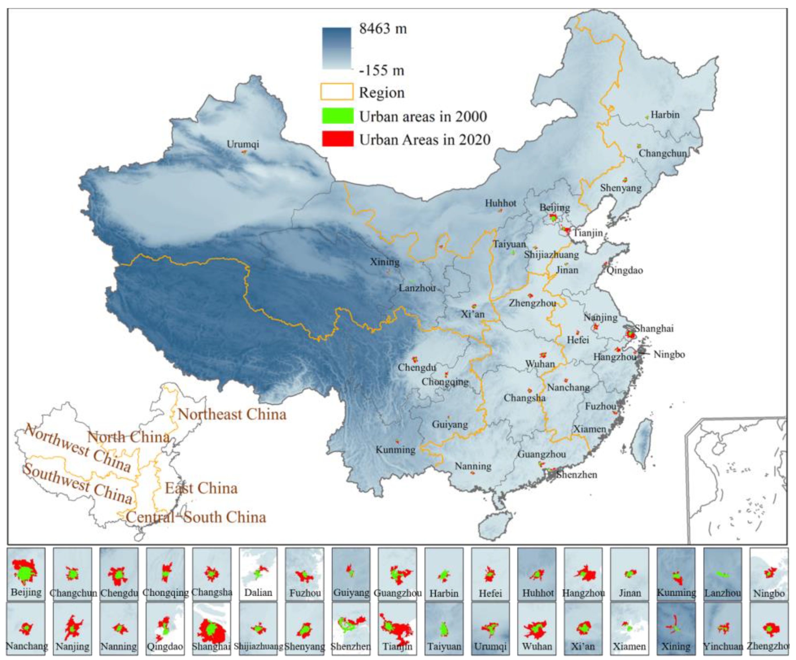
2.1. Study Areas and Data

We selected 34 major metropolitan regions across China (Figure 1). The MODIS LST product (MOD11A2) with a 1-km spatial resolution at 10:30 Beijing time from 2001 to 2020 was used to calculate daytime U H I U S and U H I U R . These LST products were improved by filtering out cloudy conditions and correcting for atmospheric water vapor, haze effects, and the sensitivity to errors in surface emissivity [52,53,54]. Global 30-m land-cover dynamic monitoring products with a fine classification system (GLC-FCS) from 2000 and 2020 were used to identify urban built-up areas. The GLC-FCS product (1985–2020, every 5 years) is produced by the Chinese Academy of Sciences using continuous time-series Landsat imagery on the Google Earth Engine platform and contains 29 land-cover types [55,56]. Impervious surfaces were regarded as built-up areas in this study. A 1 × 1 km2 grid (to be consistent with the MODIS pixel size) was created for each city. The percentage of impervious surfaces ( I S P ) was then calculated for each 1 × 1   km 2 window based on GLC-FCS data. Fifty percent of I S P was used as the threshold to identify the urban boundary in urban fringe areas [39,48]. Figure 1 shows the identified urban areas of 34 cities in 2000 and 2020.

2.2. Calculating U H I

Nine research windows, each with a size of 6 km × 6 km, were selected for each city, including one initial urban window, four emerging urban windows, and four rural windows. Figure 2 shows the spatial distribution of these nine windows. Initial urban windows remained urban and developed during 2000–2020. For most cities, four emerging urban windows were selected in their main expansion directions. However, for individual cities (e.g., Lanzhou), due to their small outward expansion areas, emerging urban windows were selected in urban fringe areas. Emerging urban windows were mainly covered by undeveloped surfaces before 2000 but were gradually replaced by urban built-up areas as cities expanded from 2000 to 2020. Rural windows represent areas that remained undeveloped during 2000–2020. They were located 5 km away from urban areas to ensure that these windows were not or were weakly affected by the U H I [41]. In each window, water bodies were excluded, and their elevation differences were within 200 m based on digital elevation model data.
U H I U S is the LST difference between the average temperature of the initial urban window and the average temperature of emerging urban windows, and U H I U R is the LST difference between the average temperature of the initial urban window and the average temperature of rural windows, calculated as:
U H I U S = T U T S
U H I U R = T U T R
where T U is the average temperature of the initial urban window, and T S and T R are the average temperatures of the emerging urban windows and rural windows, respectively.

2.3. Quantifying U B A E

To investigate the effect of U B A E on U H I , U B A E was quantified using four factors: expansion speed, proportion, compactness, and shape, which can thoroughly reflect the characteristics of landscape patches of built-up areas. Accordingly, four B A L M s were calculated for whole urban areas in 2000 and 2020 (shown in Figure 1): the annual average expansion speed of built-up areas ( A V G ), the proportion of built-up areas ( P L A N D ), the built-up patch density ( P D ), and the shape index of built-up areas ( L S I ) [57]. The P L A N D difference ( P L A N D d i f f ), P D difference ( P D d i f f ), and L S I difference ( L S I d i f f ) between 2020 and 2000 were then calculated. Combined with A V G , they were used to quantify U B A E , collectively referred to as U B A E Indices ( U B A E I s ) here.
A V G is expressed as follows:
A V G = [ U A 2020 U A 2000 ] / n
where U A 2020 and U A 2000 are the total areas of built-up patches in 2020 and 2000, respectively, and n is the year number. A larger A V G value means that U B A E is faster.
P L A N D d i f f is calculated as follows:
P L A N D = i = 1 n a i A
P L A N D d i f f = P L A N D 2020 P L A N D 2000
where a i is the area of built-up patch i , A is the total area of the research areas, and n is the number of built-up patches. P L A N D d i f f < 0 (>0) means the proportion of built-up area decreased (increased) with U B A E .
P D d i f f is expressed as follows:
P D = n / A × 10 6
P D d i f f = P D 2020 P D 2000
where n is the number of built-up patches, and A is the total area of built-up patches. A higher value of P D means more dispersed built-up areas. P D d i f f < 0 (>0) means that the built-up areas tended to be more (less) compact with U B A E .
L S I d i f f is calculated as:
L S I = 0.25 k = 1 m e i k * A
L S I d i f f = L S I 2020 L S I 2000
where e i k * is the total length (in m) of the edges between built-up patches i and k, including the entire built-up boundary and some or all background edge segments involving built-up areas. A is the total area of built-up patches. L S I = 1 when the landscape consists of a single square patch of the built-up area. L S I increases without limit as the built-up area shape becomes more irregular. L S I d i f f < 0 (>0) means that the shapes of built-up areas tended to be more (less) regular.

2.4. Quantifying the Relationship between U B A E and the Temporal Variation in U H I

The OLS regression model has been frequently used to characterize the relationship between U H I and land-use changes. It can reflect homogeneous and stationary relationships across space and is reliable for quantifying the large-scale effect of various factors on U H I and diagnosing the importance of each factor [43,50,58]. It is expressed as follows:
y = β 0 + i = 1 i β i x i + ε
where y is the dependent variable, which here is the temporal variation in U H I U S or U H I U R , quantified by the slope of the U H I fitting line (SloFL) from 2001 to 2020. β 0 is the y-intercept, β i is the local estimated coefficient of i, x i is the independent/explanatory variable i (i.e., the four U B A E I s ), i represents the number of independent variables (i.e., 4), and ε is the error term. The main output of the OLS analysis includes the coefficient of determination ( R 2 ), the p value, the coefficient of each explanatory variable, and the studentized residual (StdResid). The p value represents the overall fitness/performance of the model. The coefficients represent the strength and type of relationship between each independent variable and the dependent variable. StdResid can test the reliability of each estimated value. The closer the absolute value of StdResid is to 0, the smaller the difference between estimated and actual values. A result is unreliable when the absolute value of StdResid is larger than 2.5.
Moran’s Index (Moran’s I) was used to conduct the spatial autocorrelation test for StdResid, expressed as:
I = n i = 1 n j = 1 n W i j ( x i x ¯ ) i = 1 n j = 1 n W i j ( x i x ¯ ) 2 = i = 1 n j 1 n ( x i x ¯ ) ( x j x ¯ ) S 2 i = 1 n j = 1 n W i j
where n is the total number of cities, W i j is the spatial weight, x i and x j are the StdResids output from the OLS analyses of city i and city j , respectively, x ¯ is the average value of all StdResids, and S 2 is the variance of StdResid. Here, the global Moran’s I of StdResid was calculated to test the ability of the OLS model to address the spatial autocorrelation of variables. Results of the OLS analyses are reliable when StdResid is randomly distributed. StdResid is considered randomly distributed when the absolute value of Moran’s I is close to 0, and the Z-score is between −1.65 and 1.65.

3. Results

3.1. Geographical Distributions of U B A E I s

Figure 3 shows the spatial distributions of U B A E I s (i.e.,   A V G , P L A N D d i f f , P D d i f f , and L S I d i f f ). The average A V G of the 34 cities was 19.1 km2/year. Shanghai, the most economically developed city in China, had a maximum A V G of 76.9 km2/year. Lanzhou had the minimum A V G of 0.12 km2/year because its main urban area is surrounded by mountains, limiting U B A E . The proportion of built-up areas increased in 13 cities ( P L A N D d i f f > 0 ) and decreased in 21 cities ( P L A N D d i f f < 0 ), while the density of built-up lands increased in 12 cities ( P D d i f f < 0 ) and decreased in 22 cities ( P D d i f f > 0 ). For most cities, the densities and proportions of built-up areas increased (or decreased) synchronously. Changchun had the largest P L A N D d i f f and the smallest P D d i f f , indicating that its U B A E was primarily through infilling. However, Tianjin and Nanjing had the smallest P L A N D d i f f and the largest P D d i f f , indicating that their U B A E s were primarily through extension and leapfrog development. The shape complexity of built-up areas increased ( L S I d i f f > 0 ) in all cities except Taiyuan and Lanzhou, located in mountainous areas. Overall, in the east-west direction, A V G and L S I d i f f increased, while P L A N D d i f f and P D d i f f remained almost unchanged. In the north-south direction, A V G , P D d i f f , and L S I d i f f first increased, then decreased, while P L A N D d i f f did the opposite.
The 34 cities were divided into three types according to the topography of each city. A city was classified as a coastal city if oceans were less than 6 km away in 2020. A city was classified as a mountain city if there were mountains higher than 500 m in the vicinity. All other cities were classified as plain and hilly cities.
Figure 4a shows clear regional and topographic differences in U B A E . The U B A E of coastal cities was the most significant and fastest, as indicated by clear decreases in proportion, density, and shape regularity of built-up areas. Due to topographical limitations, the U B A E of mountain cities was the least significant and the slowest, with changes in P D and L S I also the smallest. Figure 4b shows U B A E I s in different regions. U B A E differences were consistent with differences in economic level. The U B A E s of cities in eastern, northern, and central-south China, areas with developed economies, were the fastest. The U B A E s of cities in northeast and northwest China, areas with slow-growth economies, were the slowest. The proportions, densities, and shape regularities of built-up areas decreased more markedly in cities with faster U B A E s . For cities with slower U B A E s , the proportions and densities of the built-up area increased or little changed (e.g., in the northeast and northwest China), and their shape regularities changed little.

3.2. The Geographical Distribution of U H I

Figure 5 shows the spatial distributions of average U H I U S and U H I U R in 34 cities from 2001 to 2020. Figure 6 shows U H I U S and U H I U R for different topographies and regions. On an annual basis, the average U H I U R of all cities (1.95 °C) was larger than the average U H I U S (0.73 °C). The U H I U R in the 34 cities were all positive, varying from 0.17 °C (Xining) to 3.63 °C (Chengdu). The U H I U S s in 29 cities were positive, while those in 5 cities (Qingdao, Lanzhou, Taiyuan, Guangzhou, and Xining) were negative. This means that the L S T s of emerging urban areas in these five cities were higher than those of urban areas (Figure 5(a1,b1)). Overall, the spatial patterns of annual U H I U S and U H I U R were consistent (Figure 6b). Arid cities located in northwest and north China had smaller U H I U R and U H I U S values than humid cities located in northeast, east, central-south, and southwest China (Figure 6b), attributed to the poor cooling effect caused by the sparser vegetation around arid cities compared to other cities [39]. Similar results for U H I U R were obtained in other regions of the world [8,48].
SDs in U H I U S and U H I U R were significant. Summertime U H I U R and U H I U S values were positive in all regions, but in the winter, they were negative in northwest and northern China and positive elsewhere (Figure 5(a2,a3,b2,b3) and Figure 6b). Moreover, summertime U H I U S and U H I U R values were more intense than in winter during the day, and the SDs of U H I U R were larger than those of U H I U S (Figure 5(a2–a4,b2–b4)). There are two reasons for this. First, urban spatial morphology was significantly correlated with LST in summer but not in winter [59,60]. Second, the evaporative cooling effect caused by rural vegetation was stronger in summer than in winter [39,48,61]. The SDs of U H I U R in the 34 cities were all positive, and the SDs of U H I U S in most cities were also positive, except in Urumqi and Lanzhou. This might be because the SDs in vegetation in the rural areas of these two cities are small [62]. Overall, the SD in U H I U R was significantly larger than that of U H I U S (Figure 5(a4,b4)).
Topography, land-cover type, and meteorological conditions can affect the urban L S T , altering the U H I [43,63]. Figure 6a shows U H I U S and U H I U R for different topographies. Annual and summertime U H I U R show similar patterns: the U H I U R of coastal cities was smaller than that of inland cities because sea breezes driving cold air into urban areas greatly reduced the U H I in summer [64,65]. However, in winter, the U H I U R of coastal cities was larger than that of inland cities, probably because land breezes weakening U H I circulation reduced the heat exchange between urban and rural areas, thus increasing the U H I . This needs further study.

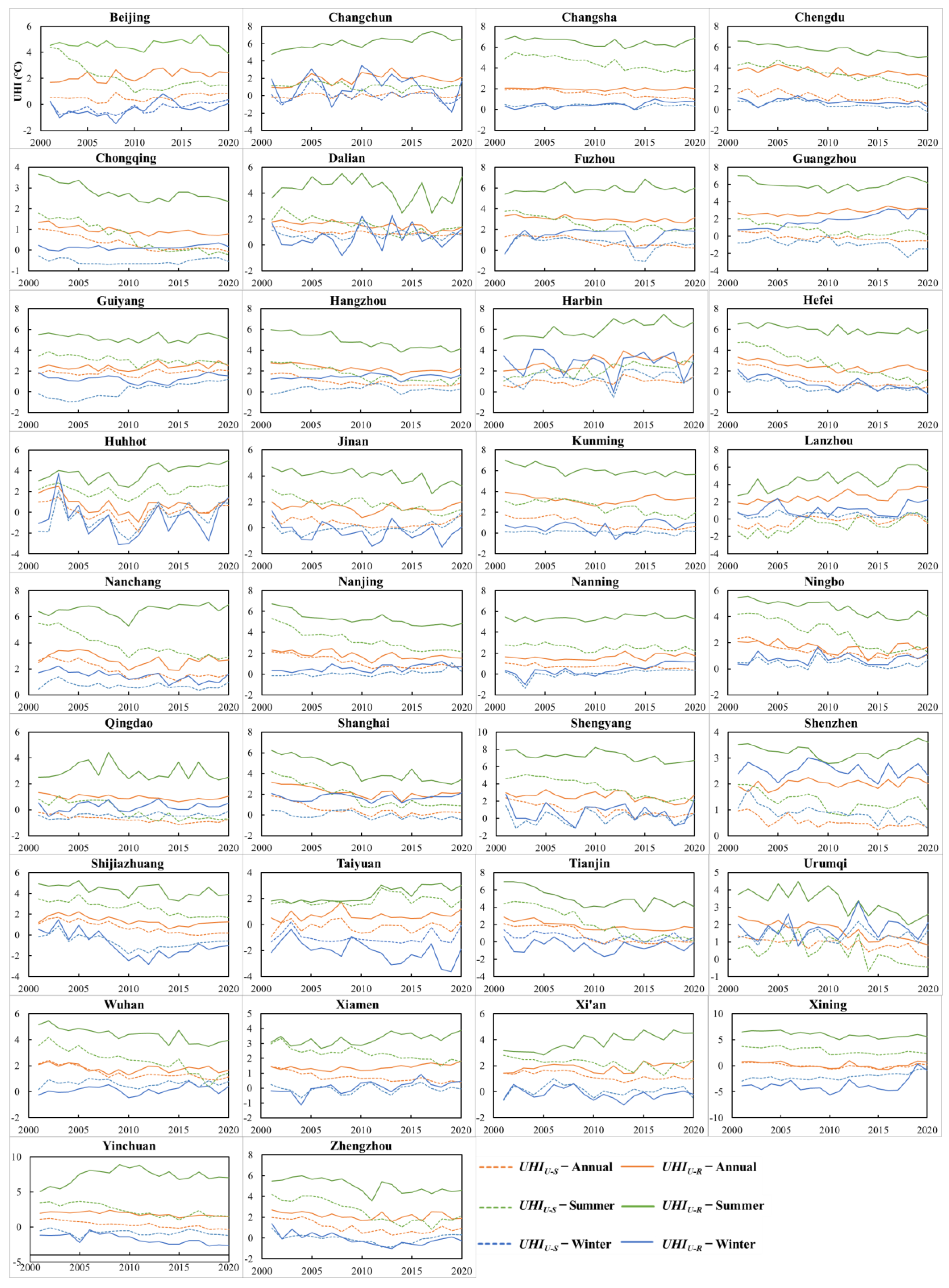
3.3. Temporal Variations in
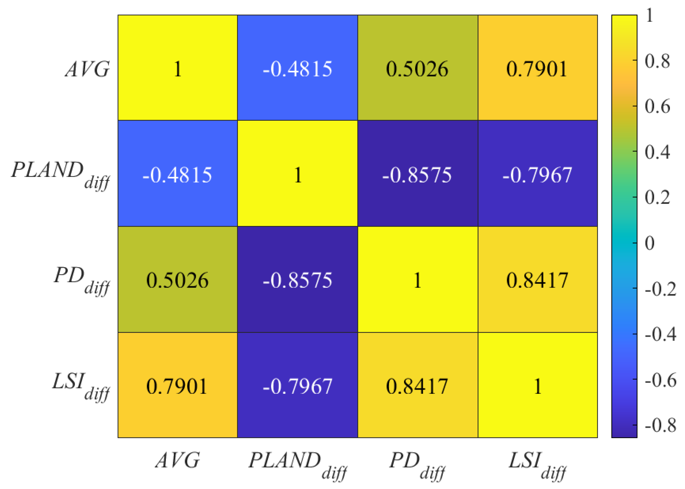
 U H I

Figure 7 shows the temporal variations in U H I U S and U H I U R in 34 cities from 2001 to 2020. The SloFL from 2001 to 2020 was used to quantify the temporal variation in U H I . A SloFL < 0 means that U H I decreases with U B A E , and a SloFL > 0 means that U H I increases with U B A E . On an annual basis, the U H I U S and U H I U R in Tianjin decreased faster (with a smaller SloFL) than in other cities, but those in Harbin and Lanzhou increased the fastest (with the largest SloFLs). This can be attributed to their opposite trends from 2000 to 2020 in P L A N D , P D , and L S I (Figure 3), discussed in Section 3.4 and Section 4. Overall, the average U H I U R in all cities decreased slightly (SloFL = −0.01), with a reduction less than that of U H I U S (SloFL = −0.05) (Figure 8(d1,d2)).
The temporal variations in U H I U S and U H I U R changed seasonally. In the summer, the U H I U S s in most cities decreased faster (with smaller SloFLs) than U H I U R except in Urumqi and Lanzhou, located in arid and rainless areas with sparse vegetation (Figure 7). Wintertime U H I U S and U H I U R showed no clear trend (Figure 7). For both U H I U S and U H I U R , summertime absolute values of SloFLs were larger than wintertime absolute values, indicating that U H I was more sensitive to U B A E in summer than in winter. Average values from all cities illustrate this: Both the U H I U S (SloFL = −0.09) and U H I U R (SloFL = −0.02) decreased with U B A E in summer and did not change (SloFL = 0) in winter (Figure 8(d1,d2)). Moreover, the SD in U H I U S between summer and winter significantly decreased with U B A E , but the SD in U H I U R changed little (Figure 8(d1,d2)).
Figure 8(a1–c1,a2–c2) show the temporal variations in U H I U S and U H I U R of cities with different topographies from 2001 to 2020. Both U H I U S and U H I U R changed more significantly in summer than in winter for the different types of cities. The variations in U H I U S and U H I U R of mountain cities differed from the other cities. Specifically, especially in summer, the U H I U S of mountain cities decreased more slowly (SloFL = −0.04) than those of coastal cities (SloFL = −0.13) and plain and hilly cities (SloFL = −0.1). The U H I U R of mountain cities increased slightly (SloFL = 0.01) while those of the other cities decreased. This can be attributed to the differences in U B A E of different types of cities, discussed next.

3.4. The Effect of U B A E on the Variation in U H I

Table 1 gives annual, summertime, and wintertime OLS results (i.e., coefficients of each U B A E I and R 2 ). Figure 9 shows StdResids outputs from the OLS model. The correlation between the U B A E I s and SloFLs of U H I (including U H I U S and U H I U R ) was stronger in summer than in winter, illustrated by the highest R 2 value that passed the significance test (Table 1) and absolute values of StdResids in all cities less than 2.5 (Figure 9(a2,b2)) in summer. This suggests that U B A E significantly affected the variation in U H I in summer but not in winter, consistent with results in Section 3.3. Results from the spatial autocorrelation test in Table 1 show that StdResid patterns were not significantly different from random in summer (i.e., Moran’s I was close to 0, and the Z-score was between −1.65 and 1.65), further suggesting that the OLS results are reliable, and that the analysis did not neglect any key explanatory variables.
Among the four U B A E I s , P D d i f f (with the largest absolute value of the coefficient) was the dominant factor affecting the temporal variation in U H I (SloFL) during U B A E , followed by P L A N D d i f f and L S I d i f f . The impact of A V G (with the smallest absolute value of the coefficient) was the least (Table 1). In summer, the relationships between U B A E I s and SloFLs were consistent for U H I U S and U H I U R , i.e., P L A N D d i f f was positively correlated with SloFL, while A V G , P D d i f f , and L S I d i f f were negatively correlated with SloFLs. Overall, the decreased density and proportion, the increased shape complexity, and the faster expansion of built-up areas accelerated the reduction in U H I and vice versa. Section 4 discusses potential factors. This indicates that in the context of continuous urban expansion, reducing the density of built-up lands is an effective way to weaken the U H I intensity [66].

4. Discussion

The representativeness of the selected urban and emerging urban windows (shown in Figure 2) to whole urban and emerging urban areas when calculating U H I was evaluated. For each city, the standard deviation of LST (LST-STD) was calculated for whole urban and emerging urban areas. The absolute value of the difference (LST-Diff) between the average LST of selected urban windows and the average LST of whole urban areas was also calculated (Figure 10). The representativeness of the selected urban windows is acceptable when LST-Diff is less than LST-STD and close to 0. For most cities, the LST-Diff was significantly less than LST-STD and less than 0.5 in all seasons, indicating that the LST of selected urban and emerging urban windows can accurately represent the LST of whole urban and emerging urban areas. The LST-Diff for individual cities (such as Fuzhou, Guiyang, Qingdao, and Xiamen) was greater than the LST-STD. The types of land use are relatively complex (with larger LST-STDs) in these cities, and there are large areas of natural surfaces (e.g., water bodies and mountainous forest parks) within their urban areas, significantly changing the average LSTs of whole urban areas. As the main focuses of this study were on built-up areas, natural surfaces were avoided when selecting urban and emerging urban windows. As a result, the LSTs of selected urban and emerging urban windows obviously differ from the average LSTs of whole urban and emerging urban areas in these cities. In conclusion, the LSTs of selected urban and emerging urban windows are sound, and the calculated U H I is reliable.
Previous studies have found that the LST spatial distribution differs in summer and winter because of the different relationships between LST and the urban spatial morphology (e.g., the density and proportion of built-up areas, the built-up fraction) [59,60]. The impact of the change in the urban spatial morphology on LST in summer was greater than that in winter, i.e., the density/fraction of built-up lands was significantly positively correlated with LST in summer but not in winter. LST varied gradually with the urban spatial morphology in summer, but there was no definite relationship in winter. The LSTs of urban fringes were even higher than those of urban centers in winter [59,60,67]. The LSTs of the initial urban area ( T U in Equations (1) and (2)) and the emerging urban area ( T S in Equation (1)) were thus more sensitive to U B A E in summer than in winter, further resulting in more significant temporal variations in U H I U S and U H I U R in summer than in winter (Figure 7 and Figure 8).
The U B A E can be classified into infilling and sprawling, and sprawling can be further divided into extension and leapfrog expansion [43]. The infilling expansion increases the density of built-up lands in the initial urban area, which can increase the LST of the initial urban area ( T U ) by enhancing surface heat storage and weakening the heat exchange between the initial urban area and its surroundings [68,69,70,71]. This has a positive effect on U H I U S and U H I U R . The sprawling expansion (especially leapfrog expansion) usually decreases the density of built-up lands, with a complex impact on LST. On the one hand, with outward urban sprawling, undeveloped surfaces (e.g., vegetated land and water bodies) around initial urban areas are gradually replaced by built-up areas (e.g., roads, buildings, and industrial parks), developing into emerging urban areas. This significantly increases the heat capacity and anthropogenic heat emissions in emerging urban areas, increasing the LST of emerging urban areas ( T S ) [72,73]. Meanwhile, the background temperature ( T R ) also increases due to the sprawling expansion [74]. On the other hand, sprawling expansion has little impact on the LST of the initial urban area ( T U ) [73,75]. This is because a city with sprawling expansion often has good planning policies and enough area for moving industrial land with high LSTs from the initial urban area to the emerging urban area. Moreover, more natural areas such as green land surfaces and parks are built in the initial urban area to improve its urban thermal environment [37,51,76], even decreasing the LST of the initial urban area ( T U ). Sprawling expansion (especially leapfrog expansion) may thus have a negative effect on U H I U S and U H I U R . If the U B A E of a city is primarily through infilling, P L A N D d i f f > 0 and P D d i f f < 0 can result. If the U B A E is primarily through sprawling, P L A N D d i f f < 0 and P D d i f f > 0 can result. So P L A N D d i f f and P D d i f f are negatively and positively correlated with the decreasing rates of U H I U S and U H I U R .
Figure 11 shows the correlation coefficient matrix of the four U B A E I s. There was a significant correlation between P D d i f f and P L A N D d i f f , i.e., the increase in proportion corresponded to the increase in density of the built-up lands. There was a positive correlation between A V G and P D d i f f and a negative correlation between A V G and P L A N D d i f f , indicating that the U B A E of a city with larger A V G was primarily through sprawling, which rapidly increased the built-up areas in emerging urban areas but reduced the overall proportion and density of built-up areas. This results in T U changing little or even decreasing but T S rapidly increasing, ultimately accelerating the decreases in U H I U S and U H I U R in summer. However, for a city with a smaller A V G , its expansion is mainly achieved by infilling, increasing the proportion and density of built-up areas in the initial urban area with a slow sprawling speed. This increases T U but slows the increase in T S , eventually attenuating the reduction in U H I U S and U H I U R . A V G is thus positively correlated with the decreasing rate of U H I . There were positive correlations between L S I d i f f and A V G , and L S I d i f f and P D d i f f , but a negative correlation between L S I d i f f and P L A N D d i f f , meaning that for a city with built-up areas increasingly complex in shape, its proportion and density of built-up areas commensurately decreased and vice versa. The increasingly complex shapes of built-up areas thus accelerated the reduction in U H I .
The U H I variations of cities located in areas with different topographies (Figure 4a and Figure 8) can be explained by the above results. The U H I U S and U H I U R of coastal cities with smaller SloFLs decreased faster than those of inland cities (Figure 8(b1,b2)) because the U B A E s of coastal cities had the smallest P L A N D d i f f and the largest A V G , P D d i f f , and L S I d i f f (Figure 4a). However, mountain cities, their U H I U S s decreased slower than the other cities, and their U H I U R s increased when the U H I U R s of other cities decreased (Figure 8(a1,a2)). This is because the A V G , P D d i f f , and L S I d i f f of mountain cities were the smallest (Figure 4a).

5. Conclusions

In this study, long-term multiple remote sensing datasets from 2001 to 2020 were used to analyze spatiotemporal variations in land surface temperature (LST) differences between urban areas and emerging urban areas ( U H I U S ) and between urban areas and rural areas ( U H I U R ) in 34 municipalities across China. Four landscape metrics of built-up area ( B A L M s ) were first calculated: the annual average expansion speed of built-up areas ( A V G ), the proportion of built-up areas ( P L A N D ), the built-up patch density ( P D ), and the shape index of built-up areas ( L S I ). Four indices were further calculated to quantify the urban built-up area expansion ( U B A E ): A V G , the P L A N D difference ( P L A N D d i f f ), P D difference ( P D d i f f ) and L S I difference ( L S I d i f f ) between 2020 and 2000, collectively referred to as U B A E Indices ( U B A E I s ). The effects of U B A E on U H I U S and U H I U R in winter and summer were further analyzed. The major findings are summarized as follows.
From 2000 to 2020, the average A V G of the 34 cities was 19.1 km2/year. Shanghai and Lanzhou had maximum and minimum A V G s of 76.9 km2/year and 0.12 km2/year, respectively. For most cities, the densities and proportions of built-up areas increased (or decreased) synchronously, and their shapes became more complex. There were significant spatial differences in U B A E . Economic development and topography impacted U B A E . The built-up areas of cities located in economically developed regions (e.g., eastern, northern, and central-south China) expanded faster, and their proportions, densities, and shape regularities decreased more noticeably than in cities located in regions with slower economic development. The U B A E s of coastal cities were the most clearly seen, with built-up areas expanding the fastest and their proportions, densities, and shape regularities experiencing the greatest decline. This was followed by plain and hilly cities, with the U B A E s in mountain cities the least noticeable.
There were clear spatial and seasonal differences in U H I U S and U H I U R . Overall, the annual average U H I U R of all cities (1.95 °C) was larger than the average U H I U S (0.73 °C), and summertime U H I U S and U H I U R were larger than those in wintertime. The seasonal difference in U H I U R between summer and winter was significantly larger than that of U H I U S . Arid cities located in northwestern and northern China had lower U H I U R s, possibly because of the weaker cooling effect caused by the sparser vegetation in rural areas. Compared with mountain cities and plain and hilly cities, the U H I U S and U H I U R of coastal cities were the lowest in summer because of the significant cooling effect caused by sea breezes. The LSTs of selected urban and emerging urban windows can well represent the LST of the whole urban areas and emerging urban areas, showing that the calculated U H I is reliable.
The temporal variations in U H I U S and U H I U R showed clear spatial and seasonal differences. On an annual basis, overall, U H I U S decreased with U B A E from 2001 to 2020, while U H I U R only slightly decreased. Both U H I U S and U H I U R in Tianjin clearly decreased, while those in Harbin and Lanzhou increased because of their opposite trends from 2000 to 2020 in P L A N D , P D , and L S I . The U H I U S and U H I U R of coastal cities decreased the fastest because the density and proportion of their built-up areas decreased the most. However, the U H I U S of the mountain cities decreased more slowly than the other cities, and the U H I U R s increased when the U H I U R s of other cities decreased because the densities of their built-up areas increased. The temporal variations in U H I U S and U H I U R were more noticeable in summer than in winter, and their relationship with U B A E was significant in summer but not in winter, indicating that the impact of U B A E on U H I U S and U H I U R in summer was more obvious than in winter.
Among the four U B A E I s , P D d i f f was the dominant factor affecting the temporal variation in U H I during U B A E . A V G had the least impact. The decreased density and proportion, the increased shape complexity, and the faster expansion of built-up areas accelerated the reductions in U H I U S and U H I U R . This indicates that during urban development, reducing the density of built-up lands by soundly planning the spatial distribution of built-up areas and natural lands can effectively weaken the U H I effect under the condition that the urban expansion speed cannot be effectively controlled.
Although this study investigated the effect of urban expansion on U H I U S and U H I U R in different seasons, the underlying intrinsic physical mechanism needs further quantitative examination using numerical model simulations. However, this is difficult to do at present because combining high spatial resolutions and long time series is a challenge for numerical modeling. We only analyzed the daytime LST in this study, so future studies should take nighttime into account to broaden our understanding. There are various methods to calculate U H I , which will be compared in future studies. The conclusions reported here are generally valid for the majority of cities studied but may not be true for all cities due to city-specific unique characteristics regarding climatic background, policies, and socioeconomic factors, among others. Focusing on a particular city could lead to valuable insights into the physical mechanisms underlying the effect of urban expansion on U H I .

Author Contributions

Conceptualization, W.H. and Z.L.; methodology, W.H. and Z.L.; validation, W.H. and Z.T.; formal analysis, W.H. and Z.T.; resources, W.H. and Z.L.; data curation, W.H., Z.T., H.F. and Q.W.; writing—original draft preparation, W.H.; writing—review and editing, Z.L., W.H., Z.T., M.C. (Miaomiao Cheng), H.F. and M.C. (Maureen Cribb); supervision, Z.L.; project administration, Z.L. and W.H.; funding acquisition, Z.L. and W.H. All authors have read and agreed to the published version of the manuscript.

Funding

This work was funded by the National Natural Science Foundation of China (grant number 42030606), the National Key Research and Development Program of China (grant number 2022YFC3703400, 2022YFC3703000), and the National Natural Science Foundation of China (grant number 42205178).

Data Availability Statement

The MODIS datasets used in this study can be freely download from https://search.earthdata.nasa.gov/. The land-cover datasets used in this study can be download from https://data.casearth.cn/.

Acknowledgments

We extend our sincerest thanks to the NASA team for their MODIS datasets and the GLC-FCS team from the Chinese Academy of Sciences for their land-cover datasets. We are very grateful to the editors and reviewers who significantly contributed to the improvement of this paper.

Conflicts of Interest

The authors declare no conflict of interest.

References

  1. Bornstein, R.; Lin, Q. Urban heat islands and summertime convective thunderstorms in Atlanta: Three case studies. Atmos. Environ. 2000, 34, 507–516. [Google Scholar] [CrossRef]
  2. Carrió, G.; Cotton, W.; Cheng, W. Urban growth and aerosol effects on convection over Houston: Part I: The August 2000 case. Atmos. Res. 2010, 96, 560–574. [Google Scholar] [CrossRef]
  3. Kaspersen, P.S.; Høegh Ravn, N.; Arnbjerg-Nielsen, K.; Madsen, H.; Drews, M. Influence of urban land cover changes and climate change for the exposure of European cities to flooding during high-intensity precipitation. Proc. Int. Assoc. Hydrol. Sci. (IAHS) 2015, 370, 21–27. [Google Scholar]
  4. Han, W.; Li, Z.; Wu, F.; Zhang, Y.; Guo, J.; Su, T.; Cribb, M.; Fan, J.; Chen, T.; Wei, J. The mechanisms and seasonal differences of the impact of aerosols on daytime surface urban heat island effect. Atmos. Chem. Phys. 2020, 20, 6479–6493. [Google Scholar] [CrossRef]
  5. Zhang, Z.; Wang, K. Quantifying and adjusting the impact of urbanization on the observed surface wind speed over China from 1985 to 2017. Fundam. Res. 2021, 1, 785–791. [Google Scholar] [CrossRef]
  6. Cao, Q.; Luan, Q.; Liu, Y.; Wang, R. The effects of 2D and 3D building morphology on urban environments: A multi-scale analysis in the Beijing metropolitan region. Build. Environ. 2021, 192, 107635. [Google Scholar] [CrossRef]
  7. Akbari, H.; Bell, R.; Brazel, T.; Cole, D.; Estes, M.; Heisler, G. Reducing Urban Heat Islands: Compendium of Strategies; United States Environmental Protection Agency (USEPA): Washington DC, USA, 2008.
  8. Peng, S.; Piao, S.; Ciais, P.; Friedlingstein, P.; Ottle, C.; Bréon, F.o.-M.; Nan, H.; Zhou, L.; Myneni, R.B. Surface urban heat island across 419 global big cities. Environ. Sci. Technol. 2012, 46, 696–703. [Google Scholar] [CrossRef]
  9. Gao, Z.; Hou, Y.; Chen, W. Enhanced sensitivity of the urban heat island effect to summer temperatures induced by urban expansion. Environ. Res. Lett. 2019, 14, 094005. [Google Scholar] [CrossRef] [Green Version]
  10. Kalkstein, L.S.; Sheridan, S.C. The Impact of Heat Island Reduction Strategies on Health-Debilitating Oppressive Air Masses in Urban Areas; U.S. EPA Heat Island Reduction Initiative Report: Berkeley, CA, USA, 2003.
  11. Centers for Disease Control and Prevention. Extreme Heat: A Prevention Guide to Promote Your Personal Health and Safety. 2004. Available online: http://www.bt.cdc.gov/disasters/extremeheat/heat_guide.asp (accessed on 27 May 2017).
  12. Taha, H.; Kalkstein, L.; Sheridan, S.; Wong, E. The potential of urban environmental control in alleviatine heat-wave health effects in five US regions. In Proceedings of the 16th Conference on Biometeorology and Aerobiology, American Meteorological Society, Vancouver, BC, Canada, 23–27 August 2004. [Google Scholar]
  13. Yow, D.M. Urban heat islands: Observations, impacts, and adaptation. Geogr. Compass. 2007, 1, 1227–1251. [Google Scholar] [CrossRef]
  14. Lu, D.; Song, K.; Zang, S.; Jia, M.; Du, J.; Ren, C. The effect of urban expansion on urban surface temperature in Shenyang, China: An analysis with landsat imagery. Environ. Model. Assess. 2015, 20, 197–210. [Google Scholar] [CrossRef]
  15. Yim, S.H.L.; Wang, M.; Gu, Y.; Yang, Y.; Dong, G.; Li, Q. Effect of urbanization on ozone and resultant health effects in the Pearl River Delta region of China. J. Geophys. Res.-Atmos. 2019, 124, 11568–11579. [Google Scholar] [CrossRef]
  16. Sarangi, C.; Qian, Y.; Li, J.; Leung, L.R.; Chakraborty, T.C.; Liu, Y. Urbanization Amplifies Nighttime Heat Stress on Warmer Days Over the US. Geophys. Res. Lett. 2021, 48, e2021GL095678. [Google Scholar] [CrossRef]
  17. Oke, T.R. The energetic basis of the urban heat island. Q. J. R. Meteor. Soc. 1982, 108, 1–24. [Google Scholar] [CrossRef]
  18. Aniello, C.; Morgan, K.; Busbey, A.; Newland, L. Mapping micro-urban heat islands using Landsat TM and a GIS. Comput. Geosci. 1995, 21, 965–969. [Google Scholar] [CrossRef]
  19. Oke, T.R. Boundary Layer Climates; Routledge: London, UK, 2002. [Google Scholar]
  20. Jiang, S.; Lee, X.; Wang, J.; Wang, K. Amplified Urban Heat Islands during Heat Wave Periods. J. Geophys. Res.-Atmos. 2019, 124, 7797–7812. [Google Scholar] [CrossRef] [Green Version]
  21. Zhao, L.; Lee, X.; Smith, R.B.; Oleson, K. Strong contributions of local background climate to urban heat islands. Nature 2014, 511, 216–219. [Google Scholar] [CrossRef]
  22. Cao, C.; Lee, X.; Liu, S.; Schultz, N.; Xiao, W.; Zhang, M.; Zhao, L. Urban heat islands in China enhanced by haze pollution. Nat. Commun. 2016, 7, 1–7. [Google Scholar] [CrossRef]
  23. Li, Y.; Wang, L.; Liu, M.; Zhao, G.; Mao, Q. Associated Determinants of Surface Urban Heat Islands across 1449 Cities in China. Adv. Meteorol. 2019, 2019, 1–14. [Google Scholar] [CrossRef] [Green Version]
  24. Yang, Q.; Huang, X.; Tang, Q. The footprint of urban heat island effect in 302 Chinese cities: Temporal trends and associated factors. Sci. Total Environ. 2019, 655, 652–662. [Google Scholar] [CrossRef]
  25. Li, T.; Cao, J.; Xu, M.; Wu, Q.; Yao, L. The influence of urban spatial pattern on land surface temperature for different functional zones. Landsc. Ecol. Eng. 2020, 16, 249–262. [Google Scholar] [CrossRef]
  26. Liu, K.; Li, X.; Wang, S.; Li, Y. Investigating the impacts of driving factors on urban heat islands in southern China from 2003 to 2015. J. Clean. Prod. 2020, 254, 120141. [Google Scholar] [CrossRef]
  27. Zhao, J.; Yu, L.; Xu, Y.; Li, X.; Zhou, Y.; Peng, D.; Liu, H.; Huang, X.; Zhou, Z.; Wang, D. Exploring difference in land surface temperature between the city centres and urban expansion areas of China’s major cities. Int. J. Remote Sens. 2020, 41, 8965–8985. [Google Scholar] [CrossRef]
  28. Yang, Q.; Huang, X.; Li, J. Assessing the relationship between surface urban heat islands and landscape patterns across climatic zones in China. Sci. Rep. 2017, 7, 9337. [Google Scholar] [CrossRef] [PubMed] [Green Version]
  29. Liang, Z.; Wu, S.; Wang, Y.; Wei, F.; Huang, J.; Shen, J.; Li, S. The relationship between urban form and heat island intensity along the urban development gradients. Sci. Total Environ. 2020, 708, 135011. [Google Scholar] [CrossRef] [PubMed]
  30. Zhang, H.; Ning, X.; Wang, H.; Shao, Z. High accuracy urban expansion monitoring and analysis of China’s provincial capitals from 2000 to 2015 based on high-resolution remote sensing imagery. Acta Geogr. Sin. 2018, 73, 2345–2363. [Google Scholar]
  31. Qiao, Z.; Tian, G.; Zhang, L.; Xu, X. Influences of urban expansion on urban heat island in Beijing during 1989–2010. Adv. Meteorol. 2014, 2014, 187169. [Google Scholar] [CrossRef] [Green Version]
  32. Pan, J. Area delineation and spatial-temporal dynamics of urban heat island in Lanzhou City, China using remote sensing imagery. J. Indian Soc. Remote 2016, 44, 111–127. [Google Scholar] [CrossRef]
  33. Shen, H.; Huang, L.; Zhang, L.; Wu, P.; Zeng, C. Long-term and fine-scale satellite monitoring of the urban heat island effect by the fusion of multi-temporal and multi-sensor remote sensed data: A 26-year case study of the city of Wuhan in China. Remote Sens. Environ. 2016, 172, 109–125. [Google Scholar] [CrossRef]
  34. Tu, L.; Qin, Z.; Li, W.; Geng, J.; Yang, L.; Zhao, S.; Zhan, W.; Wang, F. Surface urban heat island effect and its relationship with urban expansion in Nanjing, China. J. Appl. Remote Sens. 2016, 10, 026037. [Google Scholar] [CrossRef] [Green Version]
  35. Zhao, M.; Cai, H.; Qiao, Z.; Xu, X. Influence of urban expansion on the urban heat island effect in Shanghai. Int. J. Geogr. Inf. Sci. 2016, 30, 2421–2441. [Google Scholar] [CrossRef]
  36. Li, H.; Zhou, Y.; Jia, G.; Zhao, K.; Dong, J. Quantifying the response of surface urban heat island to urbanization using the annual temperature cycle model. Geosci. Front. 2022, 13, 101141. [Google Scholar] [CrossRef]
  37. Zhou, D.; Zhang, L.; Hao, L.; Sun, G.; Liu, Y.; Zhu, C. Spatiotemporal trends of urban heat island effect along the urban development intensity gradient in China. Sci. Total Environ. 2016, 544, 617–626. [Google Scholar] [CrossRef] [PubMed]
  38. Zhou, D.; Zhao, S.; Zhang, L.; Liu, S. Remotely sensed assessment of urbanization effects on vegetation phenology in China’s 32 major cities. Remote Sens. Environ. 2016, 176, 272–281. [Google Scholar] [CrossRef] [Green Version]
  39. Zhou, D.; Zhao, S.; Liu, S.; Zhang, L.; Zhu, C. Surface urban heat island in China’s 32 major cities: Spatial patterns and drivers. Remote Sens. Environ. 2014, 152, 51–61. [Google Scholar] [CrossRef]
  40. Wang, F.; Ge, Q.; Wang, S.; Li, Q.; Jones, P.D. A new estimation of urbanization’s contribution to the warming trend in China. J. Clim. 2015, 28, 8923–8938. [Google Scholar] [CrossRef]
  41. Zhou, D.; Zhao, S.; Zhang, L.; Sun, G.; Liu, Y. The footprint of urban heat island effect in China. Sci. Rep. 2015, 5, srep11160. [Google Scholar] [CrossRef] [Green Version]
  42. Peng, J.; Ma, J.; Liu, Q.; Liu, Y.; Li, Y.; Yue, Y. Spatial-temporal change of land surface temperature across 285 cities in China: An urban-rural contrast perspective. Sci. Total Environ. 2018, 635, 487–497. [Google Scholar] [CrossRef]
  43. Derdouri, A.; Wang, R.; Murayama, Y.; Osaragi, T. Understanding the Links between LULC Changes and SUHI in Cities: Insights from Two-Decadal Studies (2001–2020). Remote Sens. 2021, 13, 3654. [Google Scholar] [CrossRef]
  44. Peng, J.; Qiao, R.; Liu, Y.; Blaschke, T.; Li, S.; Wu, J.; Xu, Z.; Liu, Q. A wavelet coherence approach to prioritizing influencing factors of land surface temperature and associated research scales. Remote Sens. Environ. 2020, 246, 111866. [Google Scholar] [CrossRef]
  45. Chen, A.; Yao, L.; Sun, R.; Chen, L. How many metrics are required to identify the effects of the landscape pattern on land surface temperature? Ecol. Indicators 2014, 45, 424–433. [Google Scholar] [CrossRef]
  46. Maimaitiyiming, M.; Ghulam, A.; Tiyip, T.; Pla, F.; Latorre-Carmona, P.; Halik, Ü.; Sawut, M.; Caetano, M. Effects of green space spatial pattern on land surface temperature: Implications for sustainable urban planning and climate change adaptation. ISPRS J. Photogramm. 2014, 89, 59–66. [Google Scholar] [CrossRef] [Green Version]
  47. Liu, Y.; Peng, J.; Wang, Y. Application of partial least squares regression in detecting the important landscape indicators determining urban land surface temperature variation. Landsc. Ecol. 2018, 33, 1133–1145. [Google Scholar] [CrossRef]
  48. Imhoff, M.L.; Zhang, P.; Wolfe, R.E.; Bounoua, L. Remote sensing of the urban heat island effect across biomes in the continental USA. Remote Sens. Environ. 2010, 114, 504–513. [Google Scholar] [CrossRef] [Green Version]
  49. Zhang, P.; Imhoff, M.L.; Wolfe, R.E.; Bounoua, L. Characterizing urban heat islands of global settlements using MODIS and nighttime lights products. Can. J. Remote Sens. 2010, 36, 185–196. [Google Scholar] [CrossRef] [Green Version]
  50. Wang, L.; Hou, H.; Weng, J. Ordinary least squares modelling of urban heat island intensity based on landscape composition and configuration: A comparative study among three megacities along the Yangtze River. Sustain. Cities Soc. 2020, 62, 102381. [Google Scholar] [CrossRef]
  51. Su, H.; Han, G.; Li, L.; Qin, H. The impact of macro-scale urban form on land surface temperature: An empirical study based on climate zone, urban size and industrial structure in China. Sustain. Cities Soc. 2021, 74, 103217. [Google Scholar] [CrossRef]
  52. Wan, Z.; Dozier, J. A generalized split-window algorithm for retrieving land-surface temperature from space. IEEE Trans. Geosci. Remote Sens. 1996, 34, 892–905. [Google Scholar]
  53. Snyder, W.C.; Wan, Z.; Zhang, Y.; Feng, Y.-Z. Classification-based emissivity for land surface temperature measurement from space. Int. J. Remote Sens. 1998, 19, 2753–2774. [Google Scholar] [CrossRef]
  54. Wang, K.; Liang, S. Evaluation of ASTER and MODIS land surface temperature and emissivity products using long-term surface longwave radiation observations at SURFRAD sites. Remote Sens. Environ. 2009, 113, 1556–1565. [Google Scholar] [CrossRef]
  55. Zhang, X.; Liu, L.; Wu, C.; Chen, X.; Gao, Y.; Xie, S.; Zhang, B. Development of a global 30&thinsp;m impervious surface map using multisource and multitemporal remote sensing datasets with the Google Earth Engine platform. Earth Syst. Sci. Data 2020, 12, 1625–1648. [Google Scholar]
  56. Zhang, X.; Liu, L.; Chen, X.; Gao, Y.; Xie, S.; Mi, J. GLC_FCS30: Global land-cover product with fine classification system at 30&thinsp;m using time-series Landsat imagery. Earth Syst. Sci. Data 2021, 13, 2753–2776. [Google Scholar]
  57. McGarigal, K.; Cushman, S.A.; Ene, E. FRAGSTATS v4: Spatial Pattern Analysis Program for Categorical and Continuous Maps. Computer Software Program Produced by the Authors at the University of Massachusetts, Amherst. 2012, p. 15. Available online: http://www.umass.edu/landeco/research/fragstats/fragstats.html (accessed on 30 January 2022).
  58. Tu, M.; Liu, Z.; He, C.; Fang, Z.; Lu, W. The relationships between urban landscape patterns and fine particulate pollution in China: A multiscale investigation using a geographically weighted regression model. J. Clean. Prod. 2019, 237, 117744. [Google Scholar] [CrossRef]
  59. Lu, Y.; Yue, W.; Liu, Y.; Huang, Y. Investigating the spatiotemporal non-stationary relationships between urban spatial form and land surface temperature: A case study of Wuhan, China. Sustain. Cities Soc. 2021, 72, 103070. [Google Scholar] [CrossRef]
  60. Zhou, L.; Yuan, B.; Hu, F.; Wei, C.; Dang, X.; Sun, D. Understanding the effects of 2D/3D urban morphology on land surface temperature based on local climate zones. Build. Environ. 2022, 208, 108578. [Google Scholar] [CrossRef]
  61. Jin, M.S. Developing an index to measure urban heat island effect using satellite land skin temperature and land cover observations. J. Clim. 2012, 25, 6193–6201. [Google Scholar] [CrossRef]
  62. Piao, S.; Fang, J.; Zhou, L.; Guo, Q.; Henderson, M.; Ji, W.; Li, Y.; Tao, S. Interannual variations of monthly and seasonal normalized difference vegetation index (NDVI) in China from 1982 to 1999. J. Geophys. Res.-Atmos. 2003, 108, 4401. [Google Scholar] [CrossRef]
  63. Du, H.; Wang, D.; Wang, Y.; Zhao, X.; Qin, F.; Jiang, H.; Cai, Y. Influences of land cover types, meteorological conditions, anthropogenic heat and urban area on surface urban heat island in the Yangtze River Delta Urban Agglomeration. Sci. Total Environ. 2016, 571, 461–470. [Google Scholar] [CrossRef]
  64. Gedzelman, S.; Austin, S.; Cermak, R.; Stefano, N.; Partridge, S.; Quesenberry, S.; Robinson, D. Mesoscale aspects of the urban heat island around New York City. Theor. Appl. Climatol. 2003, 75, 29–42. [Google Scholar] [CrossRef]
  65. Yang, J.; Xin, J.; Zhang, Y.; Xiao, X.; Xia, J.C. Contributions of sea–land breeze and local climate zones to daytime and nighttime heat island intensity. npj Urban Sustain. 2022, 2, 1–11. [Google Scholar] [CrossRef]
  66. Li, W.; Cao, Q.; Lang, K.; Wu, J. Linking potential heat source and sink to urban heat island: Heterogeneous effects of landscape pattern on land surface temperature. Sci. Total Environ. 2017, 586, 457–465. [Google Scholar] [CrossRef]
  67. Coseo, P.; Larsen, L. How factors of land use/land cover, building configuration, and adjacent heat sources and sinks explain Urban Heat Islands in Chicago. Landsc. Urban Plann. 2014, 125, 117–129. [Google Scholar] [CrossRef]
  68. Li, J.; Song, C.; Cao, L.; Zhu, F.; Meng, X.; Wu, J. Impacts of landscape structure on surface urban heat islands: A case study of Shanghai, China. Remote Sens. Environ. 2011, 115, 3249–3263. [Google Scholar] [CrossRef]
  69. Zhou, W.; Huang, G.; Cadenasso, M.L. Does spatial configuration matter? 2011, 102, 54–63. [Google Scholar]
  70. Wu, H.; Ye, L.-P.; Shi, W.-Z.; Clarke, K.C. Assessing the effects of land use spatial structure on urban heat islands using HJ-1B remote sensing imagery in Wuhan, China. Int. J. Appl. Earth Obs. 2014, 32, 67–78. [Google Scholar] [CrossRef]
  71. Yue, W.; Liu, X.; Zhou, Y.; Liu, Y. Impacts of urban configuration on urban heat island: An empirical study in China mega-cities. Sci. Total Environ. 2019, 671, 1036–1046. [Google Scholar] [CrossRef]
  72. Zhang, H.; Qi, Z.-F.; Ye, X.-Y.; Cai, Y.-B.; Ma, W.-C.; Chen, M.-N. Analysis of land use/land cover change, population shift, and their effects on spatiotemporal patterns of urban heat islands in metropolitan Shanghai, China. Appl. Geogr. 2013, 44, 121–133. [Google Scholar] [CrossRef]
  73. Wu, Y.; Hou, H.; Wang, R.; Murayama, Y.; Wang, L.; Hu, T. Effects of landscape patterns on the morphological evolution of surface urban heat island in Hangzhou during 2000–2020. Sustain. Cities Soc. 2022, 79, 103717. [Google Scholar] [CrossRef]
  74. Lu, L.L.; Weng, Q.H.; Xiao, D.; Guo, H.D.; Li, Q.T.; Hui, W.H. Spatiotemporal Variation of Surface Urban Heat Islands in Relation to Land Cover Composition and Configuration: A Multi-Scale Case Study of Xi’an, China. Remote Sens. 2020, 12, 2713. [Google Scholar] [CrossRef]
  75. Carmona, P.L.; Tran, D.X.; Pla, F.; Myint, S.W.; Kieu, H.V. Characterizing the relationship between land use land cover change and land surface temperature. ISPRS J. Photogramm. 2017, 124, 119–132. [Google Scholar]
  76. Hu, D.; Meng, Q.; Zhang, L.; Zhang, Y. Spatial quantitative analysis of the potential driving factors of land surface temperature in different “Centers” of polycentric cities: A case study in Tianjin, China. Sci. Total Environ. 2020, 706, 135244. [Google Scholar] [CrossRef]
Figure 1. The spatial distribution of 34 municipal cities and 6 regions in China. Panels at the bottom show the urban areas of each city in 2000 (green) and 2020 (red), all at the same scale.
Remotesensing 15 00248 g001
Figure 2. Schematic diagram showing the spatial distribution of the research windows for a given city.
Remotesensing 15 00248 g002
Figure 3. Spatial distributions of (a) the annual average expansion speed of built-up areas ( A V G ), (b) the difference in the proportion of built-up areas ( P L A N D d i f f ), (c) the difference in the built-up patch density ( P D d i f f ), and (d) the difference in the shape index of built-up areas ( L S I d i f f ) in 34 cities between 2020 and 2000. Inset plots show results from the global spatial trend analysis, where the green and blue lines are fitting trend lines along the east-west and north-south directions, respectively.
Remotesensing 15 00248 g003
Figure 4. U B A E I s for different (a) topographies and (b) regions. Numbers in parentheses on the x-axes are the numbers of cities. Dashed lines show zero values of PDdiff.
Remotesensing 15 00248 g004
Figure 5. Spatial distributions of average U H I U S and U H I U R from 2001 to 2020 for 34 cities (unit: °C): annual (a1) U H I U S and (b1) U H I U R , summertime (a2) U H I U S and (b2) U H I U R , wintertime (a3) U H I U S and (b3) U H I U R , and seasonal differences (SDs) in (a4) U H I U S and (b4) U H I U R . SD is defined as the U H I difference between summer and winter.
Remotesensing 15 00248 g005
Figure 6. Average values of U H I U S and U H I U R for (a) different topographies and (b) regions. Numbers in parentheses on the x-axes are the numbers of cities.
Remotesensing 15 00248 g006
Figure 7. Temporal variations (annual, summertime, and wintertime) in U H I U S and U H I U R in 34 cities from 2001 to 2020. The solid and dashed lines represent U H I U R and U H I U S , respectively. Red, green, and blue colors represent annual, summertime, and wintertime results, respectively.
Remotesensing 15 00248 g007
Figure 8. U H I U S and U H I U R variations from 2001 to 2020 in mountain cities (a1,a2), coastal cities (b1,b2), plain and hilly cities (c1,c2), and all cities (d1,d2). Panel numbers 1 and 2 after the panel letters represent U H I U S and U H I U R , respectively. Red, green, and blue colors represent annual, summertime, and wintertime results, respectively.
Remotesensing 15 00248 g008
Figure 9. The StdResid distribution output from the OLS model of (a1) annual U H I U S , (a2) summertime U H I U S , (a3) wintertime U H I U S , (b1) annual U H I U R , (b2) summertime U H I U R , and (b3) wintertime U H I U R .
Remotesensing 15 00248 g009
Figure 10. LST-STDs and LST-Diffs of the 34 cities: (a) annual, (b) summertime, and (c) wintertime. LST-STD is defined as the standard deviation of LST for the whole urban area or emerging urban areas shown in Figure 1. LST-Diff is defined as the absolute value of the difference between the average LST of the selected urban window (or emerging urban windows) and the average LST of the whole urban areas (or emerging urban areas).
Remotesensing 15 00248 g010
Figure 11. The correlation coefficient matrix of urban built-up area expansion indices ( U B A E I s ).
Remotesensing 15 00248 g011
Table 1. OLS results between U B A E I s and SloFLs for different seasons. Asterisks “**” and “*” indicate 0.01 and 0.05 significance levels, respectively.
OLS ResultsSpatial Autocorrelation Test
Coefficient
AVG
Coefficient
PLANDdiff
Coefficient
PDdiff
Coefficient
LSIdiff
R2Moran’s IZ-Score
U H I U S Annual0.000717−0.001174−0.006464−0.0013210.25 *−0.1−1.68
Summer−0.0003720.000694−0.004078−0.0016850.46 **−0.069−0.92
Winter−0.001015−0.003707−0.0204910.0000890.15−0.085−1.3
U H I U R Annual0.0002880.00134−0.004557−0.0004210.20 *−0.042−0.28
Summer−0.000320.001986−0.00233−0.0014280.50 **−0.045−0.35
Winter−0.00079−0.001234−0.0285360.0013450.040.0511.95
Disclaimer/Publisher’s Note: The statements, opinions and data contained in all publications are solely those of the individual author(s) and contributor(s) and not of MDPI and/or the editor(s). MDPI and/or the editor(s) disclaim responsibility for any injury to people or property resulting from any ideas, methods, instructions or products referred to in the content.

