

FARMSAR: Fixing AgRicultural Mislabels Using Sentinel-1 Time Series and AutoencodeRs

1
SONDRA, CentraleSupélec, Université Paris-Saclay, 3 Rue Joliot Curie, 91190 Gif-sur-Yvette, France
2
DTIS, ONERA, 6 Chemin de la Vauve aux Granges, 91120 Palaiseau, France
*
Author to whom correspondence should be addressed.
Remote Sens. 2023, 15(1), 35; https://0-doi-org.brum.beds.ac.uk/10.3390/rs15010035
Submission received: 24 October 2022
/
Revised: 15 December 2022
/
Accepted: 17 December 2022
/
Published: 21 December 2022
(This article belongs to the Special Issue AI Datasets, Tools, and Specifications for Earth Observation Applications)
Abstract
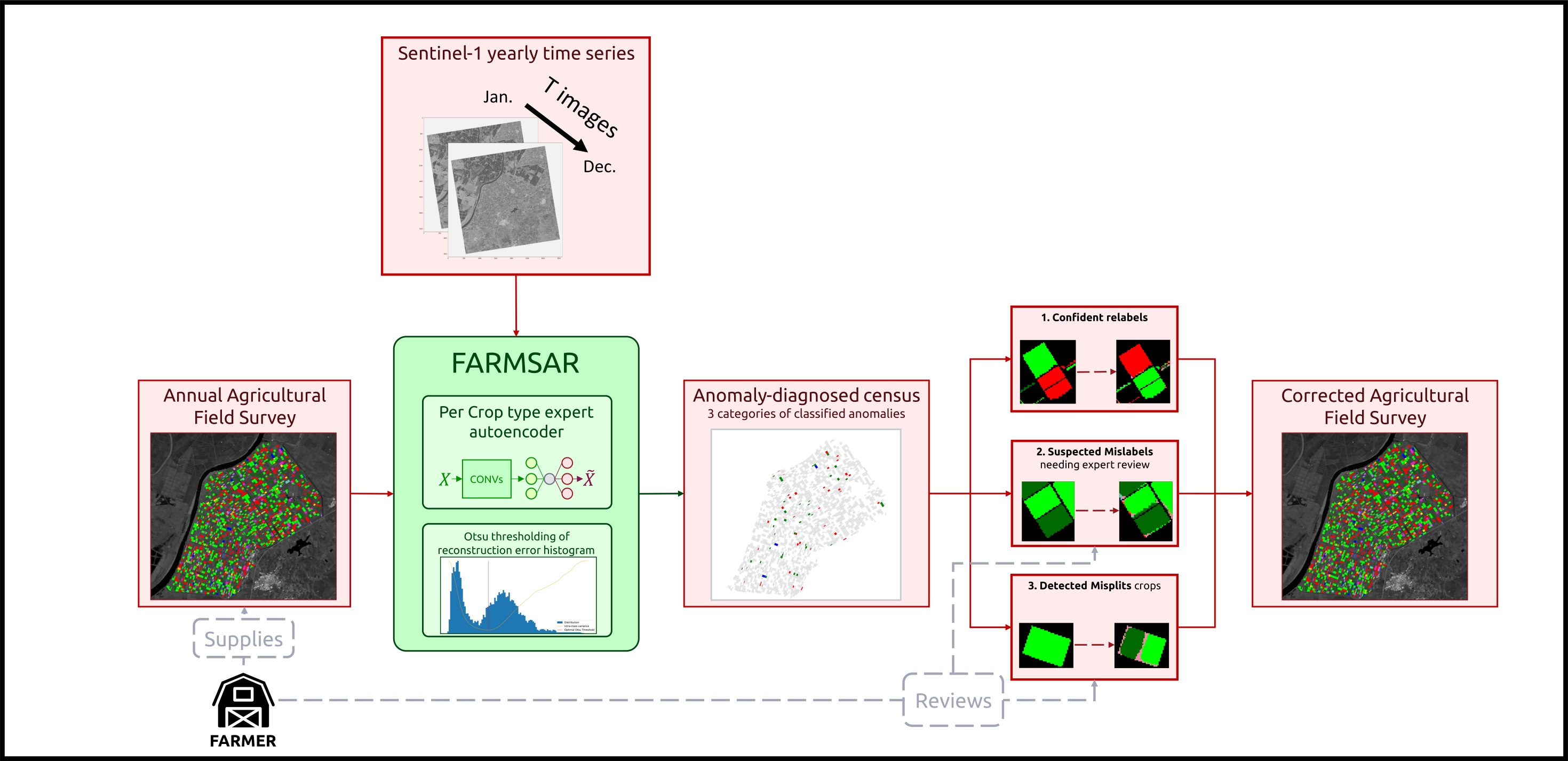
:This paper aims to quantify the errors in the provided agricultural crop types, estimate the possible error rate in the available dataset, and propose a correction strategy. This quantification could establish a confidence criterion useful for decisions taken on this data or to have a better apprehension of the possible consequences of using this data in learning downstream functions such as classification. We consider two agricultural label errors: crop type mislabels and mis-split crops. To process and correct these errors, we design a two-step methodology. Using class-specific convolutional autoencoders applied to synthetic aperture radar (SAR) time series of free-to-use and temporally dense Sentinel-1 data, we detect out-of-distribution temporal profiles of crop time series, which we categorize as one out of the three following possibilities: crop edge confusion, incorrectly split crop areas, and potentially mislabeled crop. We then relabel crops flagged as mislabeled using an Otsu threshold-derived confidence criteria. We numerically validate our methodology using a controlled disruption of labels over crops of confidence. We then compare our methods to supervised algorithms and show improved quality of relabels, with up to 98% correct relabels for our method, against up to 91% for Random Forest-based approaches. We show a drastic decrease in the performance of supervised algorithms under critical conditions (smaller and larger amounts of introduced label errors), with Random Forest falling to 56% of correct relabels against 95% for our approach. We also explicit the trade-off made in the design of our method between the number of relabels, and their quality. In addition, we apply this methodology to a set of agricultural labels containing probable mislabels. We also validate the quality of the corrections using optical imagery, which helps highlight incorrectly cut crops and potential mislabels. We then assess the applicability of the proposed method in various contexts and scales and present how it is suitable for verifying and correcting farmers’ crop declarations.

1. Introduction
Historically, remote sensing data, and in particular, synthetic aperture radar (SAR) data have been used in support of agricultural processes: their sensibility to the physiological state of crops enabled the monitoring of their growth [1,2,3] or the classification of crop types, with supervision [4,5,6,7] or without [8,9,10]. SAR temporal data over optical or hyperspectral data allows for continuous worldwide monitoring, regardless of weather conditions. Furthermore, the launch of Sentinel-1 satellites, with free-to-use and open data of up to 6 days of time-interval between acquisitions, favors the increased use of SAR for agricultural monitoring. Recently, SAR has been combined with deep learning technologies [11,12] for the task of agricultural monitoring, which allow for improved performance, and generalization, over traditional approaches.
Said applications usually rely on agricultural labels, which may come with a significant amount of label noise [13,14]. This label noise can have a non-negligible impact on decision-making for agricultural policies, as they “misinform key statistics and hence grand development programs”, according to [15]. Thus, tackling label noise is critical, for downstream tasks relying on highly qualitative agricultural data.
Deep learning algorithms can extract label noise, such as mislabels, using anomaly detection frameworks [16,17]. According to [18], anomalies correspond to an observation that “deviates so significantly from other observations as to arouse suspicion that it was generated by a different mechanism”. Thus, the extraction of label noise relies on anomaly detection methodology, which can be split into mainly three categories:
- supervised anomaly detection, where a model is trained to detect anomalies that are labeled as such. Such an approach is prevalent in medical applications for novelty detection [19]. However, having a labeled anomaly dataset is rare, and such a training paradigm is not robust against unexpected anomalies.
- semi-supervised anomaly detection [20,21]: labels of anomalies and normal instances are still present but in a significant imbalance. In this context, deep autoencoders [22] are used. They are unsupervised deep learning models trained with a reconstruction task. In a semi-supervised context, they are trained only on normal observations. Then, deviating instances are used to fit a reconstruction performance threshold above which anomalies can be separated from the norm. However, despite requiring a much lower amount of anomalies than supervised anomaly detection, there is still a need for such labels. If there is no anomalous label on hand, one must use unsupervised anomaly detection.
- unsupervised anomaly detection [23]: methodologies of this kind train deep autoencoders in the same way, but without knowledge of which data point is normal and which is an anomaly. The distinction between the two classes is entirely made from data and is much harder to find. However, it is much more robust to new unseen kinds of anomalies.
In remote sensing, anomaly detection algorithms have been applied to a various range of earth observation applications, such as sea monitoring [24], vegetation anomaly detection [25] or the problem at stake: agricultural monitoring [26]. In our work, we primarily focus on label anomalies: in particular, mislabels. Their detection and correction in remote sensing context is the topic of multiple studies. Santos et al. [27] presents a class noise quality control method in the context of land cover classification of satellite time series using self-organizing maps. Wang et al. [28] detect and correct label noise in a target recognition context using training loss curves of deep learning models to characterize, extract and classify outliers.
A particular kind of remote sensing data anomaly we are interested in is crop type anomaly. Di Martino et al. [9] studies the retrieval of agricultural classes from SAR time series using unsupervised algorithms. We uncover a series of crops labeled as “cotton” which appear closer to “sugar beets”, both in terms of optical reflectance and radiometry. However, this work does not automatically detect and correct mislabels. For that, Avolio et al. [29] presents a methodology that uses satellite image time series and dynamic time warping to compare a given NVDI temporal signature with per-class trends. However, the usage of optical imagery to characterize plant growth patterns is sensitive to clouds and atmospheric conditions [30]. In addition, such trends may not be discriminative enough to separate crop types.
In an alarming agricultural context worldwide, it becomes crucial to find solutions to prevent the transmission of agrarian census errors and to optimize the efficiency of agronomic measures. In this paper, we present a candidate solution for the task of diagnosing agricultural census quality and correcting labeling mistakes by combining remote sensing data and a custom deep learning anomaly detection and correction algorithm, with the three following contributions to the literature:
- we use deep convolutional autoencoders to model, without supervision, the expected temporal signature of crops in Sentinel-1 multitemporal images.
- we leverage the reconstruction performance of autoencoders as a class belongingness measure and present an automatic binary thresholding strategy for confidence relabeling using Otsu thresholding [31].
- we combine time series-level and parcel-level analysis to better extract and correct anomalies.
We first present our methodology by introducing the context of the illustrating use case and the multi-stage FARMSAR algorithm (Fixing AgRicultural Mislabels using Sentinel-1 time series and AutoencodeRs). We validate the proposed methodology in a controlled environment. We isolate the labels of trustworthy time series within a first half of the dataset and randomly introduce mislabels. We then run our method, and we numerically quantify the mislabel retrieval and correction performance for quantitative analysis of our method’s performance. We repeat this process multiple times, with varying amounts of introduced label errors, for statistical relevance. We then apply FARMSAR to the second half of the available dataset, supporting the presented corrections and diagnostics using qualitative validation with Sentinel-2 imagery.
2. The Stakes in Agricultural Ground Truths
2.1. The Value of Ground Truths
Agricultural ground truth products are of interest to various bodies, including public institutions and scientists. Indeed, in Angus et al. [32], the World Bank details the importance of agriculture for national and international economic development. Agricultural policy frameworks are in place in every region of the world. For instance, in Europe, the Common Agricultural Policy of the European Union (CAP) supports farmers with subsidies to improve the quantity and quality of agricultural production. In return, farmers need to declare crop parcels with information on location and harvest. The European Union then uses the reports to ensure that it is self-sufficient in food production of various kinds. Institutions take advantage of agricultural censuses to support their decisions with quantitative arguments. This reporting process is part of a general approach by the European Commission to digitize agricultural information. It involves the creation, among other things, of the Land Parcel Identification System.
On the other hand, agricultural labels are crucial for the work of scientists in various fields, including Agronomy, Ecology, and Earth Sciences. In particular, in remote sensing, agricultural labels can help in crop type mapping applications at different scale: local [5], national [33] or continental [34]. These applications use trusted ground truths to fit a classification model that predicts an agricultural label for unseen areas. The quality of these predictions is a function of the quality of the training datasets. The presence of label noise in these datasets is directly connected to the creation of these crop surveys.
2.2. The Difficulties of Building Agricultural Datasets
Both authorities and farmers encounter many difficulties during and after crop survey completion. For instance, Beegle et al. [35] shows complications regarding the reliability of recall in agricultural data collected from a variety of sources. Further studied by Wollburg et al. [36], there exists a non-negligible correlation between survey question recall length and measurement errors in agricultural censuses. The authors also detail the impact of these errors on agricultural variables, key to decision making for administrations.
On another hand, Tiedeman et al. [13] shows the impact of data collection methods on crop yield estimations based on Sentinel-2 images analysis, comparing farmer estimated ground truth and true measured ground truth. Their results point towards the idea that the design of the survey process in itself can lead to the introduction of errors [37].
Depending on the use of these agricultural labels, the impacts of label noise are various.
2.3. The Impacts of Errors in Ground Truth Data
While errors in agricultural surveys are explicable, they remain damaging for both institutions and scientists. For instance, Abay [15] shows the direct impact of plot size overestimation on the returns to modern agricultural inputs, which directly support the decision process of institutions to invest in new agronomic technologies. The presence of errors, intentional or not, is a matter of interest to authorities such as the Italian government, which mandated Avolio et al. [29] to develop a tool for compliance checks of farmers’ declarations.
Remote sensing applications such as crop type mapping or yield estimation also suffer from label noise. In the presence of errors in the training ground truths, the model will damage the predictions with approximations. Indeed, knowing the impact of errors in annotated databases on learning algorithms is also a topic of interest. Some works have shown that below a certain threshold of errors, and for sufficiently large learning bases, the impact is negligible [38]. However, this conclusion does not necessarily extend to all scenarios, especially those for which the learning bases are too small, not diversified enough, or when the learning techniques are weakly supervised.
For instance, in the context of Land Cover mapping [38], a sharp decline in performance appears after 20% of label noise. In another context, in the context of crop type mapping with NDVI time series, Pelletier et al. [14] shows the impact of errors in agricultural training labels which become non-negligible when reaching more than 20% of label noise.
Thus, having a criterion to qualify potential errors could therefore be of interest to conduct a parametric study to better study their impact. The types of label noise encountered in an agricultural setting are multiple. In our work, we focus on label noise errors, that we now introduce and characterize.
2.4. Ontology of Studied Crop Type Errors
The concept of an agricultural survey previously introduced can be seen as a dataset of parcels that has the following characteristics:
- Each parcel is atomic, because they are not supposed to be dividable into smaller parcels.
- The atomicity of parcels is assured by the homogeneity of the crop type: every part of the parcel contains the same plant. We can then assign to the field this crop type as a class.
From these two axioms may arise errors that must, at least, be detected and, at best, be corrected. The first type of error regards the supposed atomicity of the parcel; the parcel consists of two sub-parcels. We call this error “mis-split parcel”. The second type of error regards the assigned crop type; the assigned crop type is not the real crop type. We call this error “mislabeled parcel”.
The axioms presented above are valid within a single unit of time, defined by the harvesting strategy of the farmer. We are working with a time unit of 1 year (i.e., year-long crop rotations), but the presented method stays valid for any other crop rotations scheme.
Building on this axiomatic representation of crop type errors, we develop a methodology entitled FARMSAR: Fixing AgRicultural Mislabels using Sentinel-1 time series and AutoencodeRs.
3. The FARMSAR Methodology
3.1. SAR Temporal Modeling of Crops, a Study Case of Sector BXII, Sevilla
Mestre-Quereda et al. [5] shows the ability of SAR backscatter time series to perform crop type mapping. In particular, Sentinel-1 satellites offer numerous advantages regarding their usage for agricultural monitoring. Their capacity to perform exploitable acquisitions no matter the weather, their high temporal resolution (from 6 to 12 days), and high availability make it an ideal candidate for continuous crop monitoring.
This article illustrates our methodology with a dataset of Sentinel-1 acquisitions over agricultural fields of Sector BXII, a farming area located near Sevilla, Spain. Sector BXII is a group of farmers gathered under the concept of community irrigation [39], which increases the efficiency of water usage through a bulk supply of water to the agricultural fields from a given source. With a total of 1128 members in 2018, the community is frequently under the radar of local and national Spanish governments for its experimental irrigation technology. For that matter, errors in crop census are detrimental to decision-makers at various levels of responsibility.
The Sentinel-1 multitemporal stack was processed as presented by Mestre-Quereda et al. [5] and consists of 61 acquisitions during the whole year of 2017. The processing includes in particular a boxcar speckle filter of 19 samples in range, and 4 samples in azimuth, performed before geocoding, which results in anomalies we present later. We display in Table 1 the metadata of the acquisitions.
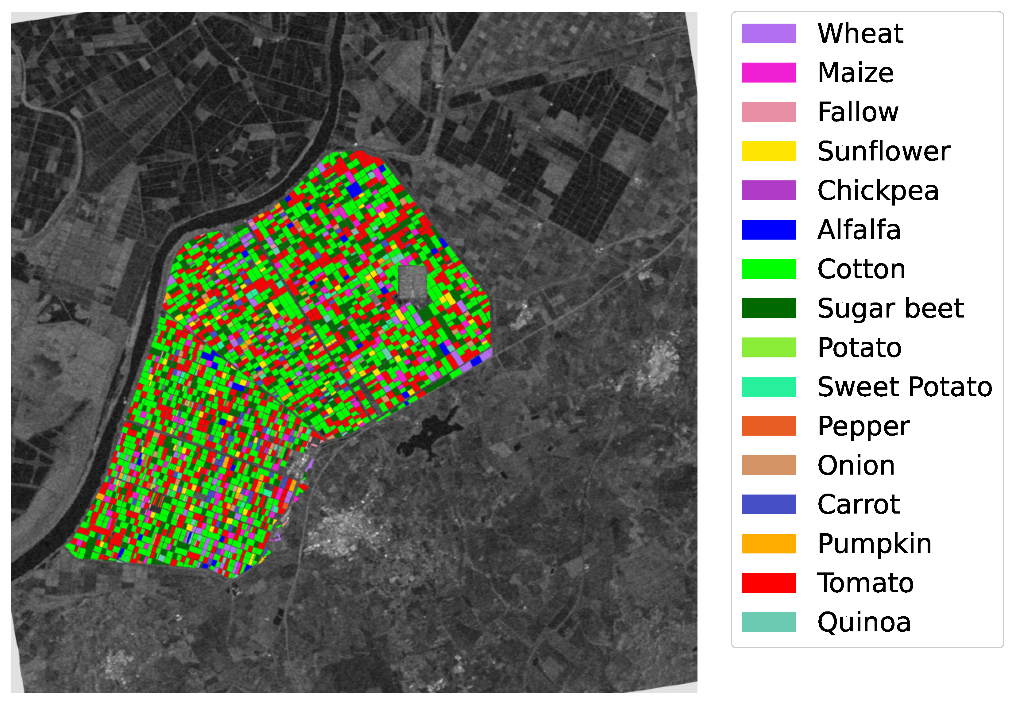
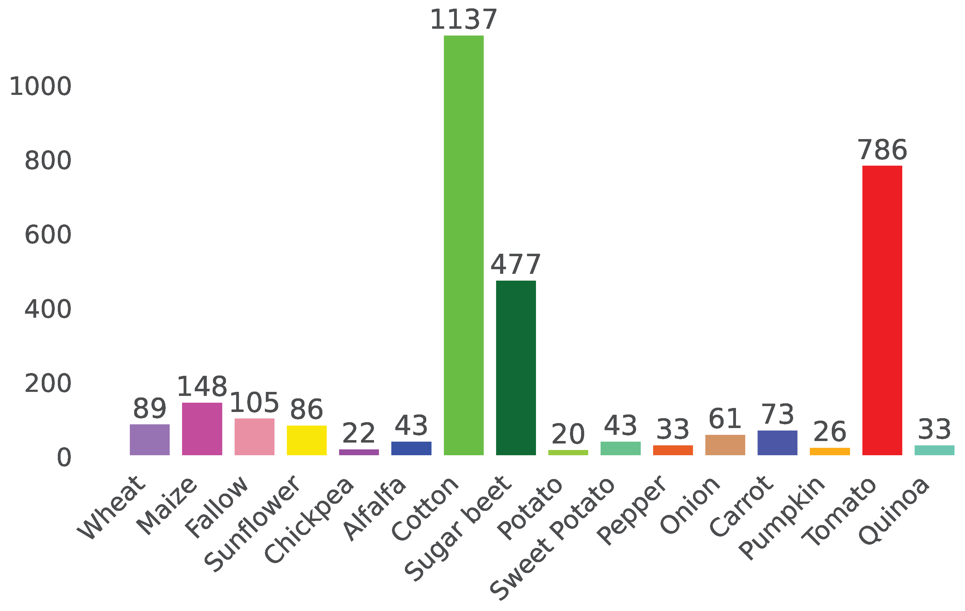
Illustrated in Figure 1, 16 crop types act as labels for the Sentinel-1 time series, with a total of around 3200 unique crops and 1.2M pixel-wise time series. These labels were created by farmers of Sector BXII and correspond to the annual harvest classes of 2017. The main products of the sector are sugar beet, tomato, and cotton. Further details regarding crop types distribution are displayed in Figure 2.
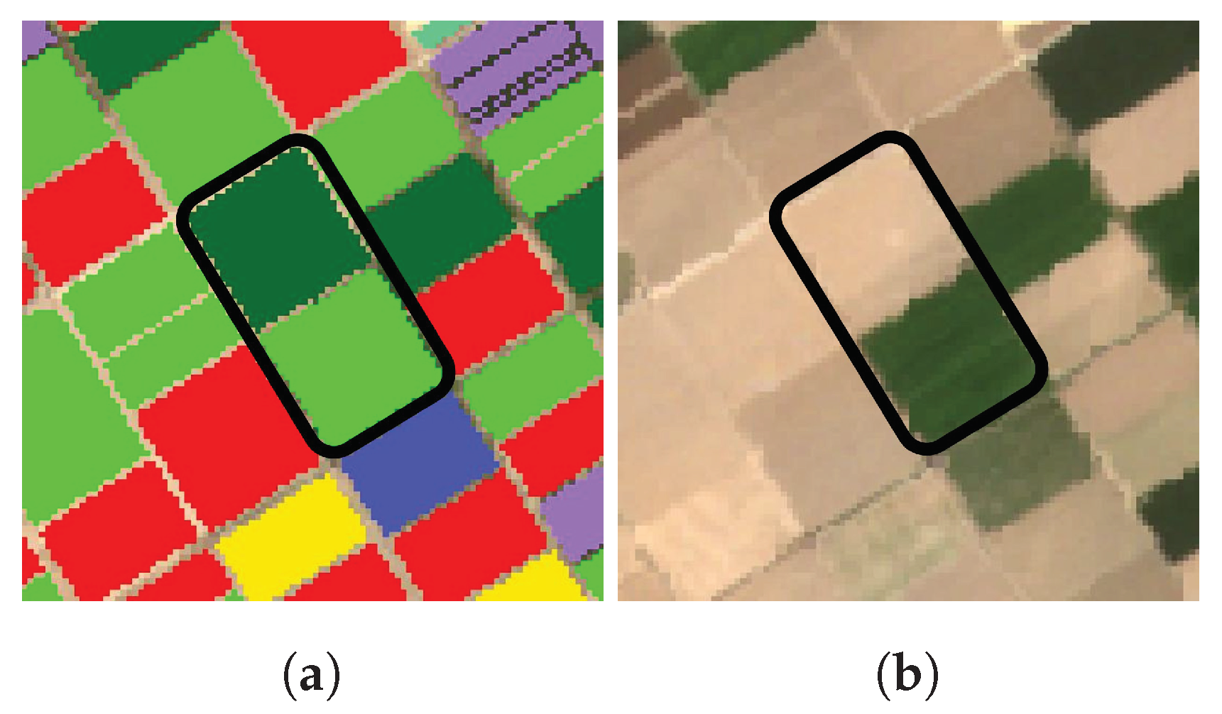
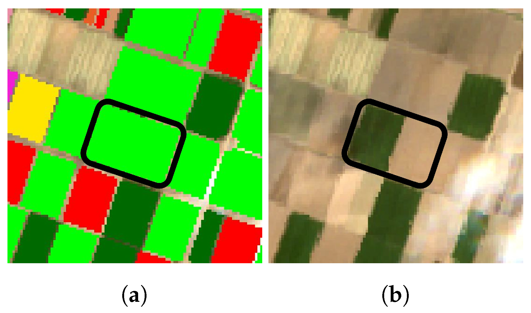
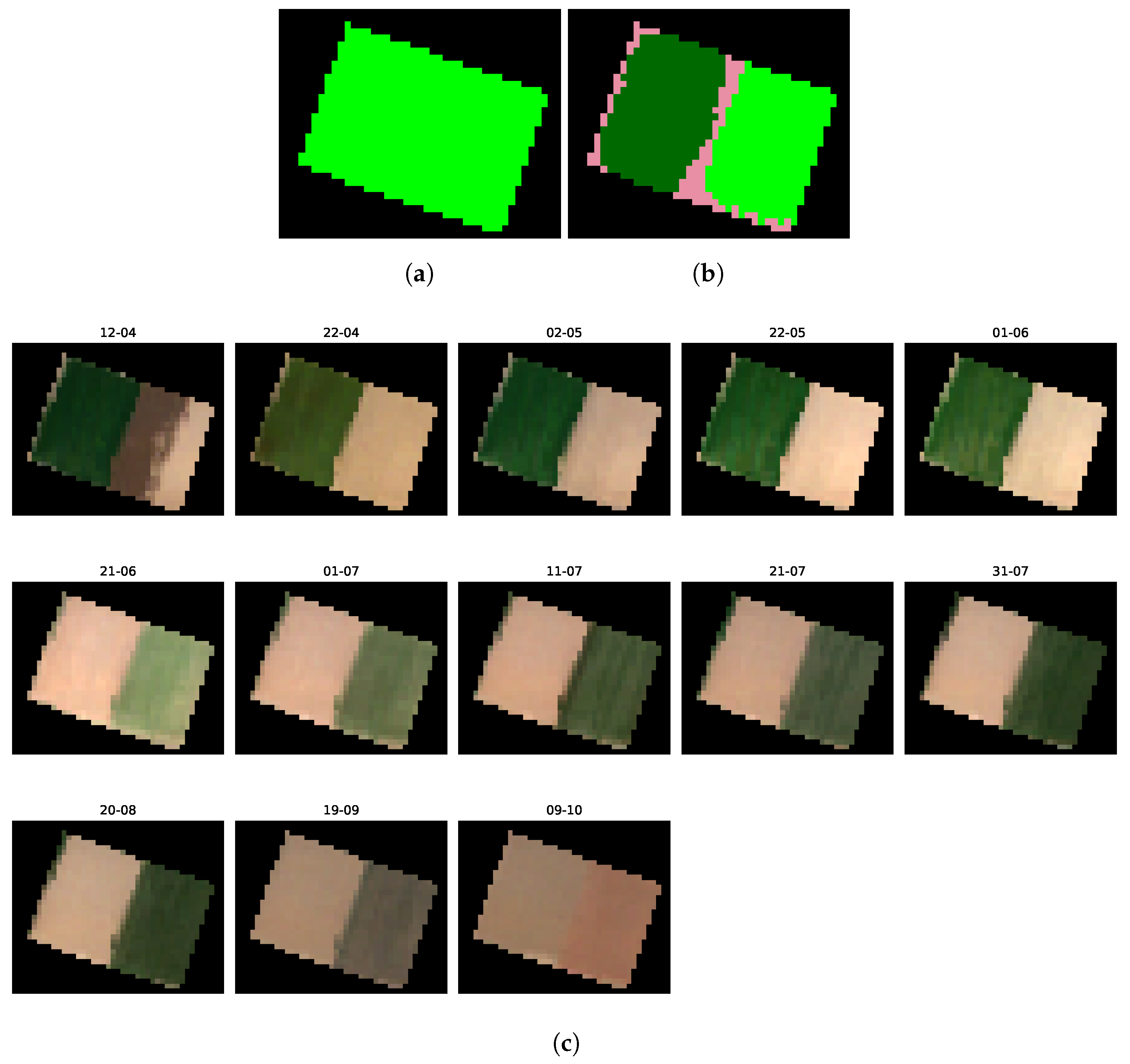
This Sector BXII crop survey contains labeling errors, and we illustrate examples of these mistakes in Figure 3 with the display of suspected mislabels and in Figure 4 with the display of a supposed mis-split crop. When observing the aspect of the suspect beet crop in Figure 3b, it appears very dissimilar from other neighboring beet crops. Considering that the 22nd of April is during the beet growing season in the Sevilla region, it seems highly unlikely for this crop to be beets. Conversely, the second suspect crop, labeled as cotton, appears green on the same image, despite the cotton growing season happening over the summer (June–August). These remarks lead us to believe that both of these crops are of the wrong label. When observing the crop highlighted in Figure 4b, it appears heterogeneous in the 22nd of April image, making it a suspected mis-split crop.
More suspicious crops are scattered within the agricultural area. However, with more than 3000 crops, it becomes complex and time-consuming to double-check all their labels individually and verify the atomicity of each parcel.
Thus, this paper details an automatic correction process of the labels of this dataset with the support of Sentinel-1 time series. The validity of relabels are then assessed quantitatively using controlled degradation of labels of crops we consider as “trustworthy” as well as qualitatively using Sentinel-2 optical imagery.
For presentation and validation purposes, we have split the available crops into two groups:
- A first group, representing 50% of the crops (field-wise), is used for quantitative validation of the methodology. In this group, we filter out any suspicious crop, with a process that we detail in the following sections, only to keep crops with high confidence in the veracity of their labels. We then perform repeated random introduction of label errors ten separate times for accurate statistical and numerical evaluation of the proposed methodology. The reader may also find details of this process in the validation section.
- A second group, representing the other 50% of the crops, illustrates the methodology workflow and is corrected. We extract what FARMSAR classifies as mis-split and mislabeled crops and evaluate the appointed corrections qualitatively using Sentinel-2 imagery.
3.2. Convolutional Autoencoder for SAR Time Series
In the context of noisy labels, unsupervised algorithms help to gain insights entirely from data without disruption from mislabeled samples. Indeed, considering the tasks of detecting mis-split and mislabeled crops as well as being able to correct mislabels, we need a method that models both dissimilarity, to detect anomalies within a class, and similarity, to correct anomalies. Unsupervised learning methodologies can be used to perform these detections and corrections.
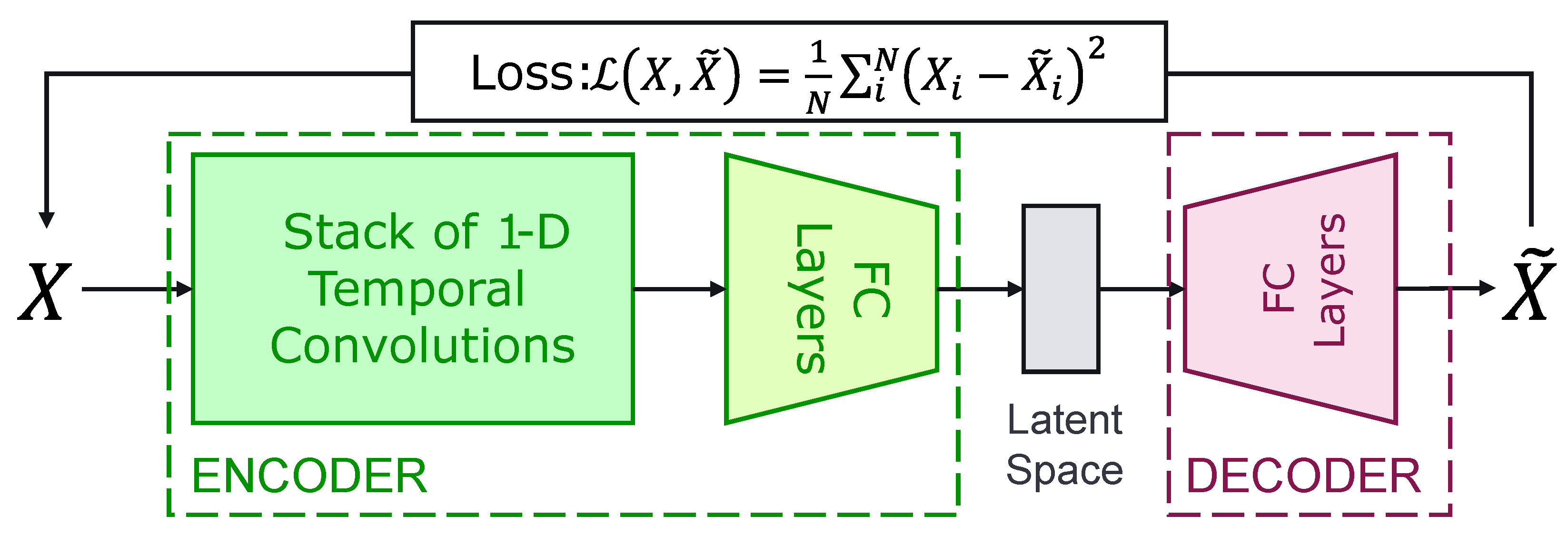
In particular, Convolutional Autoencoders (CAE) are used to model a dataset’s distribution. CAEs are a Deep Learning model consisting of two components, as shown in Figure 5; a convolutional encoder and a decoder:
- The convolutional encoder uses convolutions to extract temporal features from the input time series that are then transformed by a stack of fully-connected layers (FC Layers), with Exponential Linear Unit (ELU) activation functions [40], and projected onto an embedding space of low dimension.
- The decoder consists of a stack of fully-connected layers, combined with ELU activation functions, tasked with reconstructing the original time series, from the embedding space representation, through a mean square error loss function computed between the input time series and the output of the decoder.
The architecture used for our version of the CAE is detailed in Table 2.
Formally, the forward pass of a CAE can be written as:
where is the weight matrix of the encoder and is the weight matrix of the decoder. The loss used to train a CAE, can then be expressed as:
This mean-square error loss, also called “reconstruction error”, clarifies the training task of the network, which is to recreate the input time series after its compression in the embedding space. This bottlenecking strategy forces the autoencoder to extract discriminative features from the input data and then encode it into a lower-dimension vector. The recreation task that follows the compression can help detect outliers: in-distribution data points will be relatively better reconstructed than anomalies, to the condition that said anomalies are in the minority compared to the norm. Using a threshold over the MSE value of every data point, we can separate the anomalies from the norm. Thus, the reconstruction mean-squared error of a time series and a well-defined thresholding strategy are an efficient anomaly detection criteria.
The CAEs architectures are developed using PyTorch 1.10.2, and trained on an RTX 5000 with 16 GB of VRAM, alongside 64 GB of RAM and an Intel Xeon W-2255 CPU.
3.3. Detection of Mis-Split and Mislabeled Crops
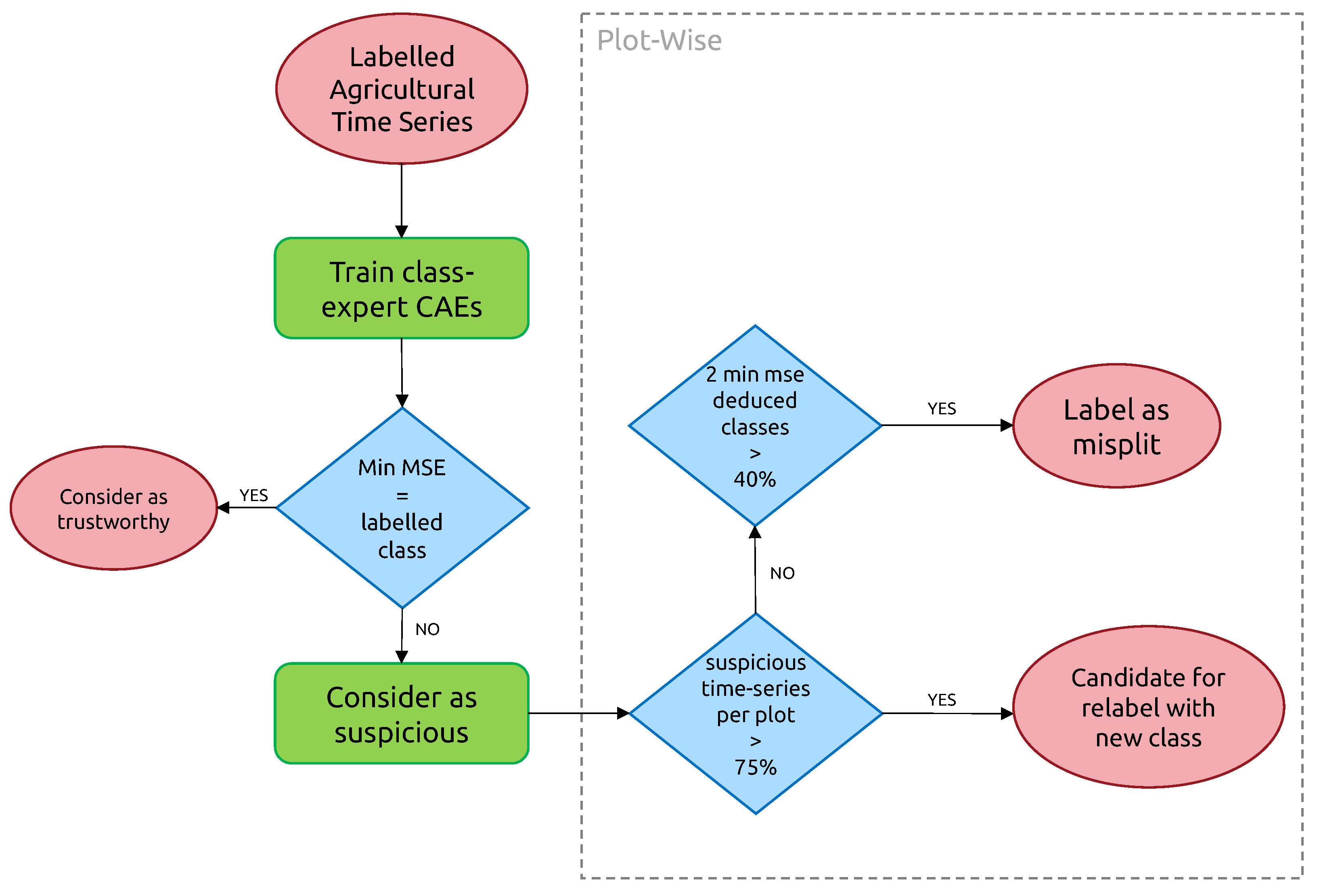
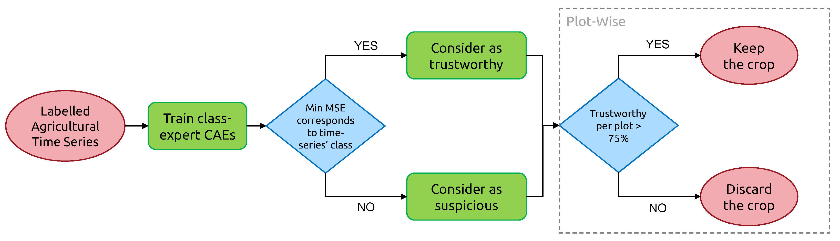
As described in Figure 6, the whole methodology consists of a series of steps: first, we work at pixel-wise time series-level and extract “suspicious” time series. Then, we gather them at the crop-level and decide, using various thresholding strategies, whether the whole parcel is mislabeled, mis-split, or neither. In the following subsections, we go over the details of these two steps.
3.3.1. Iterative Training of Class-Expert CAEs
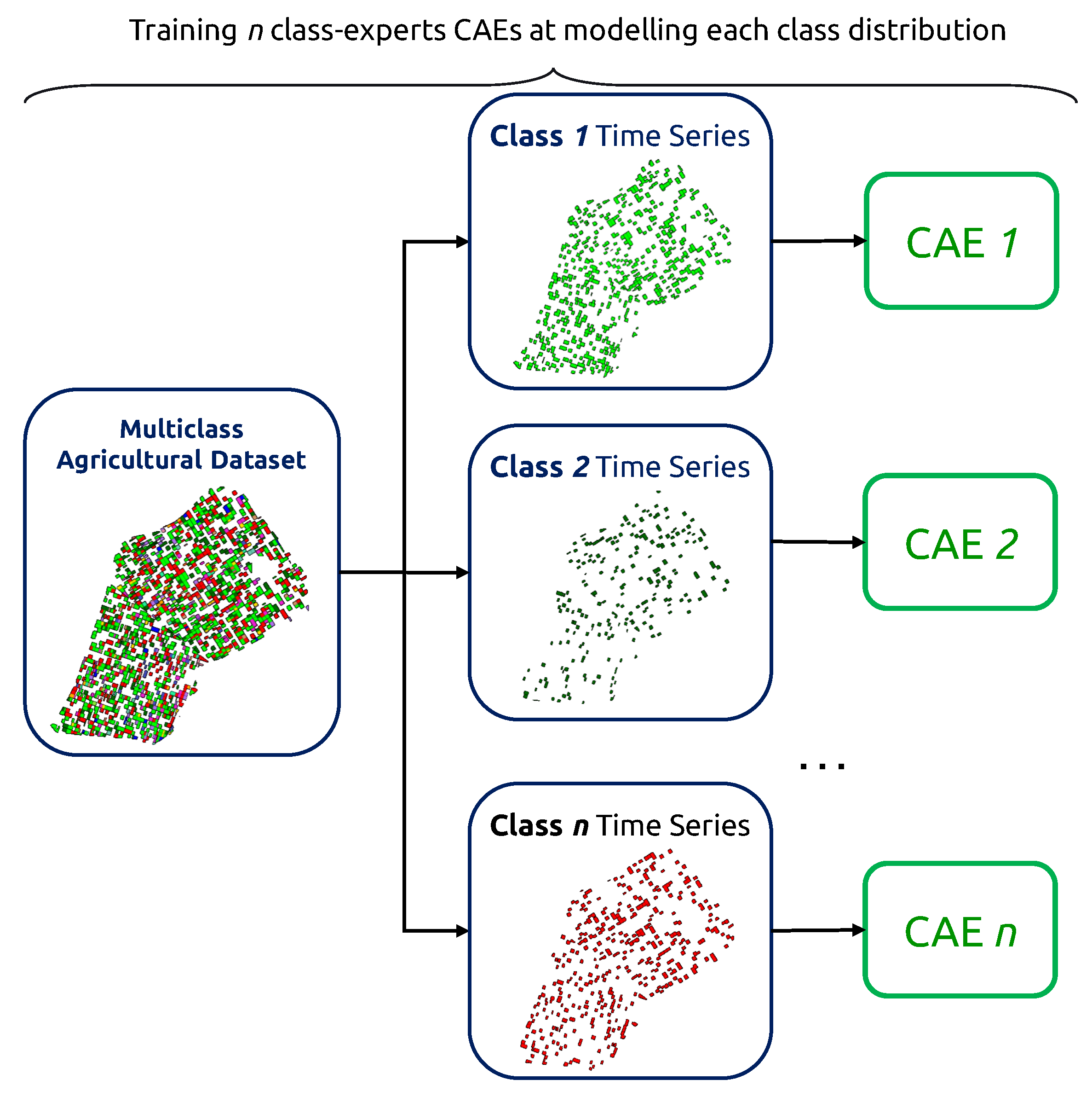
The first step of our methodology consists in flagging what we call “suspicious” agricultural pixel-wise time series. The suspiciousness criteria can be defined using an anomaly detection scheme: finding the anomaly within the norm. In the context of multiclass labeling, we need to account for the presence of a variety of norms. We employ class-expert CAEs: multiple Convolutional Autoencoders, each trained exclusively on time series of their respectively assigned class. For that, we use the original classes of the supplied dataset.
Given a survey with n crop types, we then obtain n CAEs, as shown in Figure 7. Each CAE is designed with an embedding dimension of 1 to ensure the strictest bottlenecking possible for improved outlier detection. The training process of CAEs is summarized in Algorithm 1, and training parameters are displayed in Table 3.
| Algorithm 1 Iterative training of CAE, with removal of suspicious elements |
|
For improved detection of suspicious elements, we retrain, from scratch, class-expert CAEs with a refined dataset, where previously suspicious pixel-wise time series have been removed. This iterative process allows different degrees of outliers extraction: from easier to find in the first iterations to more complex in the last. We iterate 10 times over the dataset, performing progressive filtering of suspicious elements. While we could have used a stop criterion, we found an iteration-based solution to be more flexible for the diversities in profile distributions of each class.
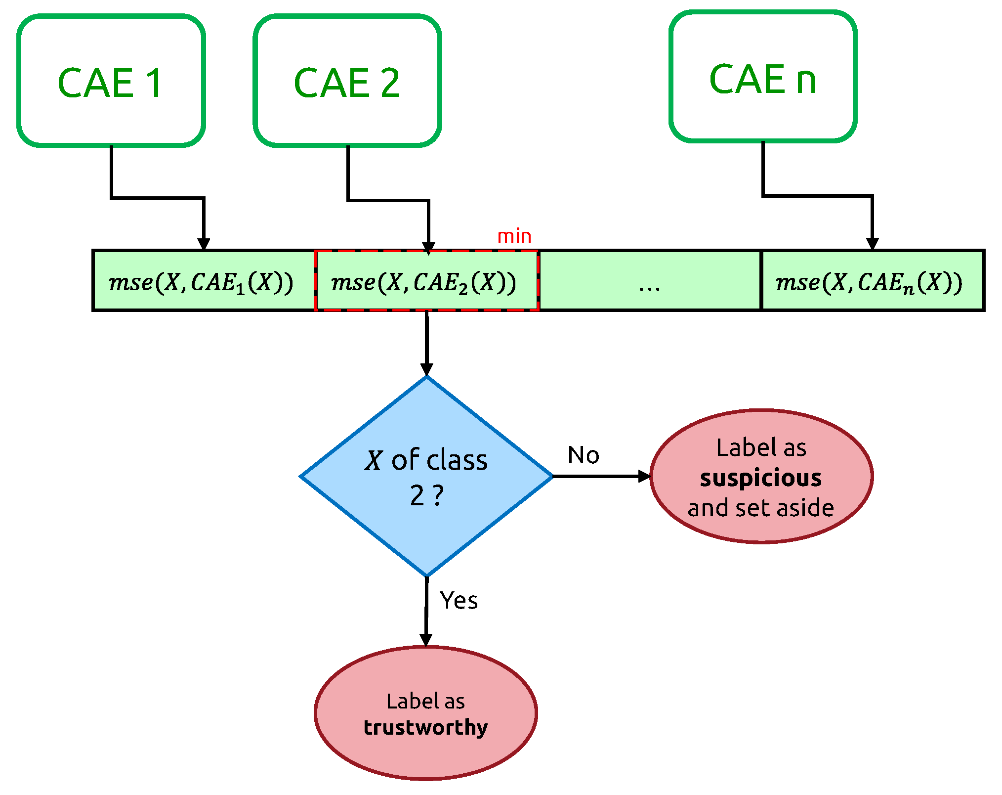
The decision to identify an input time series as suspicious relies on a vector of mean-squared errors (cf. Figure 8), one per class-expert CAE.
From now on, we call the “candidate new class” of X. If this candidate new class does not correspond to the original ground truth class of the input time series, we label this time series as “suspicious”, “trustworthy” otherwise.
After the first iteration of the assignation of “suspicious” and “trustworthy” labels, the suspicious elements of each class are set aside, and we start a new training of class-expert CAEs from scratch, only with “trustworthy” time series. We iterate this process ten times.
After the last iteration, we obtain a list of “suspicious” time series that we use to detect plot-level anomalies.
3.3.2. Plot-Level Classification of Time Series Anomalies
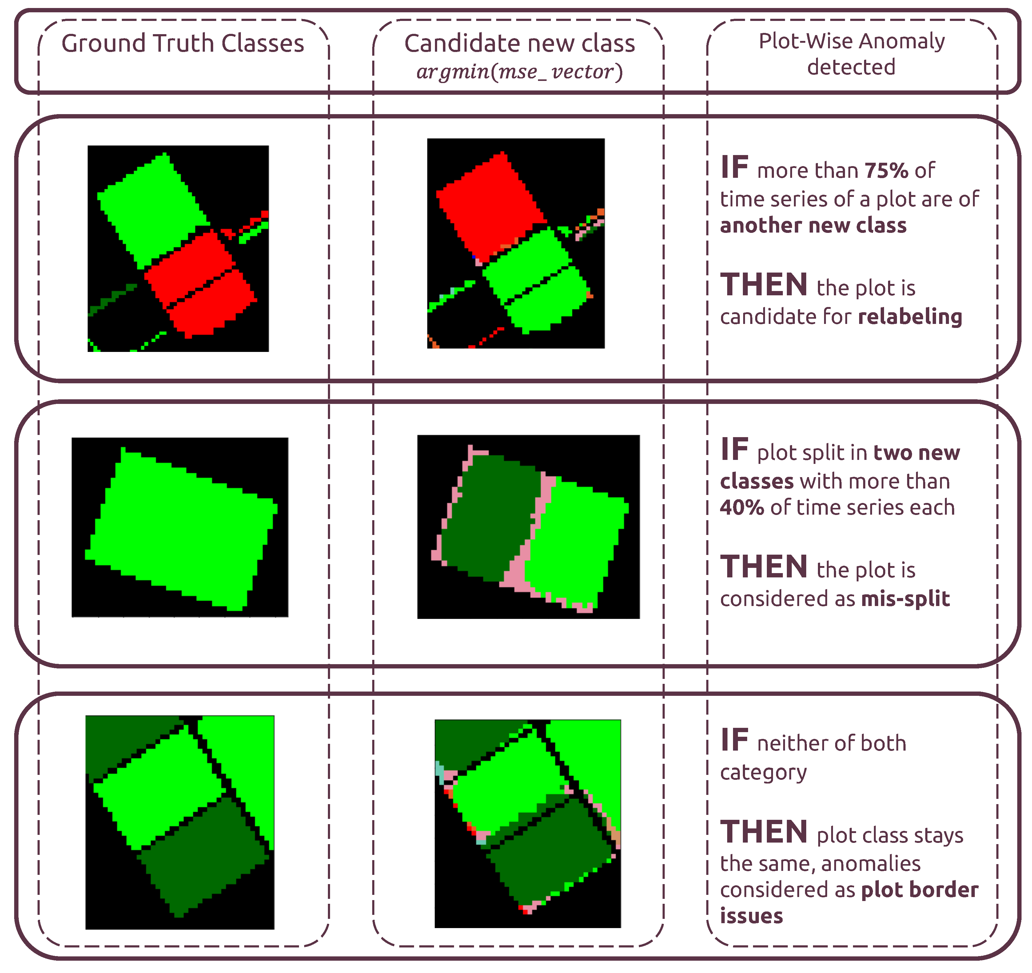
For plot-level classification of anomalies, 3 outcomes are possible, as shown in Figure 9:
- “Candidate for relabeling”: we consider a plot as a candidate for relabeling when more than 75% of the pixel-wise time series within the field are of the same new class. We empirically chose the value of 75% as “edge cases“ can represent up to 20% of the time series-level mislabels within a field. Allowing a margin of error of approximately 5%, we thus reach the threshold of 75%.
- “Mis-split plot”: we consider a plot as “mis-split” if two different classes are present with the crops boundaries, according to each time series’ candidate new class, with each representing at least 40% of the plot size. The 40% criteria is also empirically found, as a field composed of at least two candidates classes, each representing 40% of its inner time series, will have 80% categorized as candidates classes, leaving up to 20% of the rest to potential edge cases.
- “Edge Cases”: we consider any other time series-level anomaly as edge cases. We believe they arise for multiple reasons, including differences in resolution between the labels and the satellite imagery, the preprocessing of Sentinel-1 data, which included boxcar despeckling, or approximate incorrect geolocation of labels/SAR data.
Now that we have extracted candidates for relabeling, we present a confidence-based methodology to assign, or not, a new class to the mislabeled crop plots.
3.4. Correction of Mislabeled Crops
Used until then to detect class anomalies, the reconstruction performance of CAEs can also serve as a measure of class belongingness. Indeed, having a minimum reconstruction performance from a CAE trained on data from another class does not necessarily mean that the current plot is of the wrong class and that this new class is a better fit. Thus, we need this confidence-based methodology to ensure the following two points:
- The prior class of a given time series is not correct (i.e., class outlier detection). We model this using .
- A given time series belongs to the new candidate class (i.e., class belongingness detection). We model this using .
Class outlierness and belongingness are antagonistic measures, so we opt for a single binary thresholding strategy, providing a reconstruction threshold below which we consider belongingness and above which we consider outlierness. For that, we use histogram-based thresholding with the Otsu Method, developed by Otsu [31]. Initially introduced for the transformation of gray-level images into black and white images, this methodology allows for separating a histogram with two spikes. It searches for a binary threshold that results in the smallest intra-class variance, averaged over the two groups. We can formulate this idea with Equation (3):
where , , with being the standard deviation function and (empirical probability that X is equal or below ), (empirical probability that X is above ).
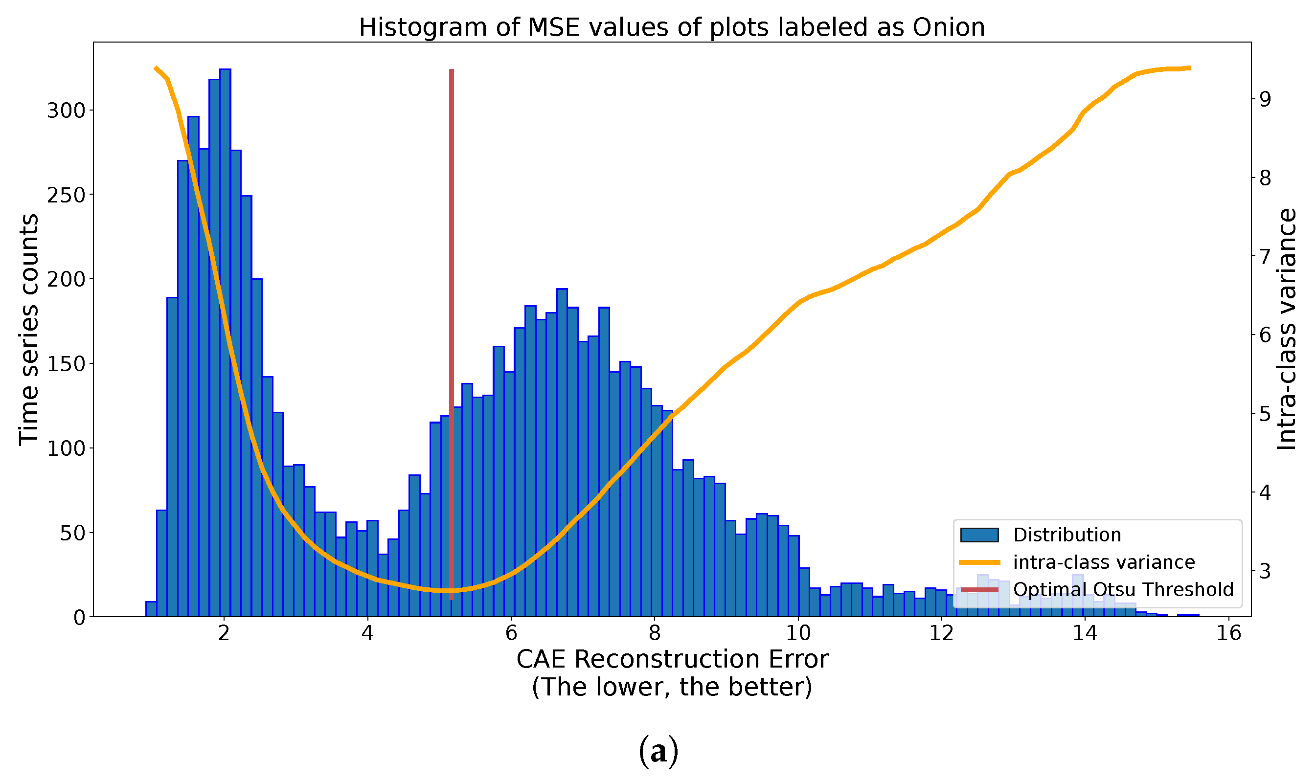
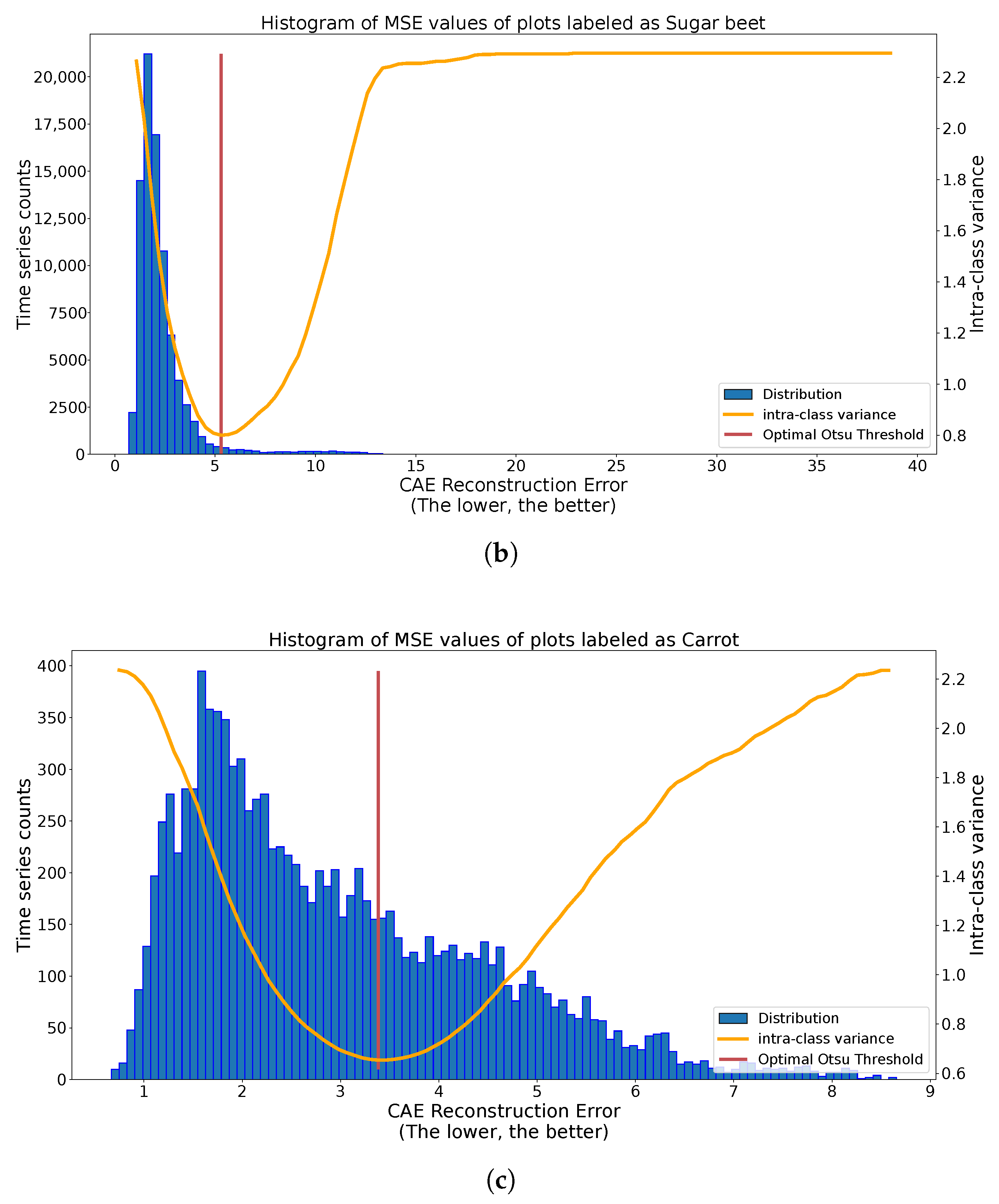
We can observe in Figure 10 the results of the application of the Otsu methodology on different class histograms with different distributions. In the case of Figure 10a, we observe two clear spikes with various spread. The found threshold significantly separates these two spikes. In the case of Figure 10b, we have many more labeled plots, inducing a more skewed histogram. Despite this, the Otsu thresholding method separates the central spike of reconstruction from outlier values. For the last case, with carrots, in Figure 10c, there is no clear threshold above which outliers are present. The quality of the threshold method depends on the quality of separation of outliers by the autoencoders, or even on the presence on outliers. Under the harder conditions of Figure 10c, the Otsu methodology splits the histogram into two dense regions. These three situations illustrate good automatic thresholding results, extracting candidate outliers on one side and, on the other side, candidate true labels.
Thus, to validate relabeling, we verify if these two formulas hold for the crop at hand:
- Check that the parcel is among the least well reconstructed of its ground truth class, i.e., .
- Check that the parcel is among the best reconstructed of its new class,i.e., .
This double-check strategy ensures that relabels are performed only with high confidence.
To validate the presented methodology on the dataset of Sevilla crops, we first turn to quantitative validations using the controlled disruption of labels.
4. Numerical Validation of the Methodology
To validate the FARMSAR method presented before, we first opt for quantitative validation to measure the expected error rate in the relabeling process. For that, we design a custom and controlled experimental environment.
4.1. Quantitative Validation Scheme: A Controlled Disturbed Environment
To measure the label correction performance of our methodology, we need the ground truth of introduced label errors: i.e., errors that we produce ourselves, from original labels in which we have a high degree of trust. For that, we need to filter out from this half of the dataset any potential mislabel and mis-split crop.
Illustrated in Figure 11, the method used to extract trustworthy crops is based on the same method as the one used to extract suspicious crops: we keep every crop with more than 75% of their time series considered as trustworthy, i.e., where the CAE performing the best reconstruction in terms of mean-square error is of the same class as the input time series. The threshold of 75% is empirical and is also deduced from the observation that edge cases anomalies may represent up to 25% of the area of a crop. As a result, out of the 1588 available crops, we keep 1008, for which we have high confidence in their label.
After building our dataset of high-confidence labels, we now randomly introduce label errors repeatedly in different amounts. In total, we run ten experiments. We introduce errors for 1, 5, 10, 15, 20, 25, and 30% of the labels and run our methodology on these error-riddled datasets. We run these experiments ten times for statistical relevance of the retrieved performance.
4.2. Correction Performance, a Comparison with Supervised and Unsupervised Methods
To justify the use of our methodology for the correction of mislabels, we compare the performance of our method against supervised (Random Forests, Linear Support Vector Classifier) and unsupervised methods (CAE without Otsu thresholding verification of relabeling candidates).
Supervised algorithms are trained using a 4-folds cross-validation process, on flattened time-series (122 sized vectors instead of the original 61 × 2 multimodal vector): a first model is trained on 75% of the data and performs predictions on the 25% left. Any prediction diverging from known labels is considered a relabel prediction. If the algorithm relabels more than 75% of a crop, the entire crop is then relabeled.
Taking into account the context of diagnosing the quality of an agricultural labeling process, we consider two performance metrics:
- How many mislabels are correctly relabeled?This metric offers a measure of how many mislabels we expect to miss, given the chosen method. It provides an approximate of how many mistakes may be remaining in the cleaned crop type survey (without taking into account mistakes that may be added by the correcting algorithms themselves).
- Out of every relabels, how many are correct?Given a set of corrections, this metric provides an estimate of how many are erroneous. In other words, it is similar to estimating how many mistakes are introduced by the correcting algorithm.
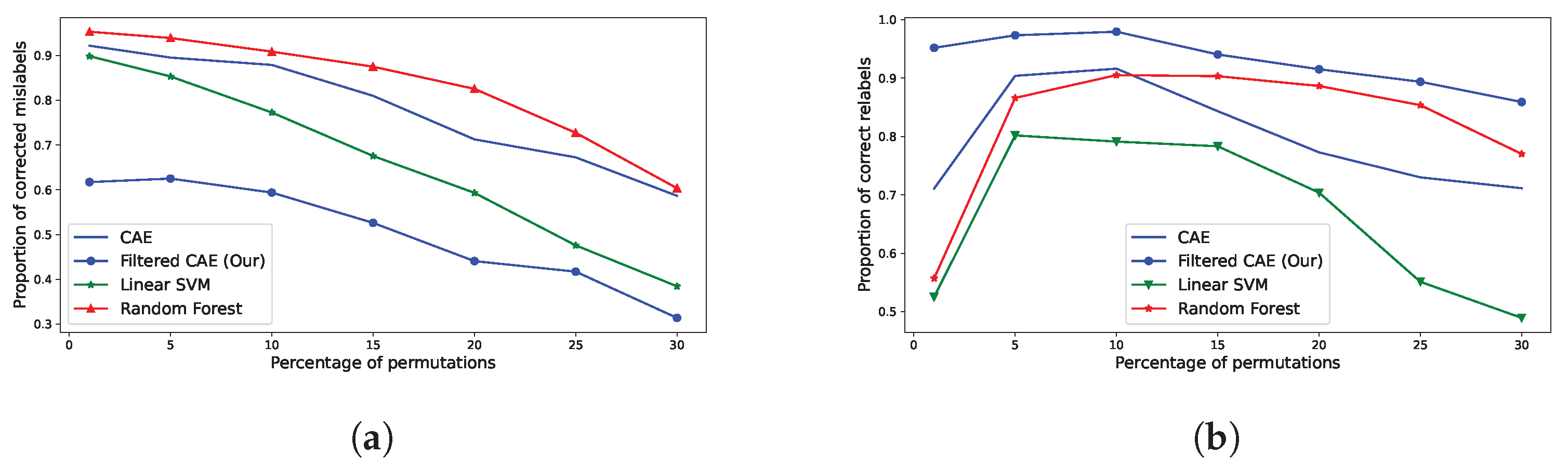
As illustrated in Figure 12 and Table 4, we observe a concrete performance distinction between our proposed method and other methodologies. Indeed, while fewer relabels are corrected overall (cf Figure 12a), the quality of the relabels is critically improved (cf Figure 12b). For example, in a case of 10% of mislabels within an agricultural census, if our methodology suggests a relabel, there is only 2% chance that the suggested relabel is incorrect, against 9% for Random Forest-based methodologies, 8% for vanilla-CAE and 21% for Linear SVMs.
In addition, the amount of correct relabels from supervised methodologies is at its worst for low amounts of mislabels introduced (1%). In other words, the less there is to correct, the more supervised methods introduce mistakes. In comparison, such methodologies make almost twice more relabeling mistakes than our methodology: 56% of correct relabels for Random Forest against 95% of proper relabels for our methods. This gap between methods is inherent to the supervised nature of Random Forest and Support-Vector Machines, where it becomes hard to distinguish relabeling candidates from classification errors. Indeed, by training our CAEs with no classification task, we explicitly fit them with modeling each class’s norm, improving their performance at extracting deviating crops.
With these metrics, we strengthen the validation of relabels using our methodologies, and we explicit the trade-off made with our method: fewer relabels overall but a higher quality of relabels. This trade-off is however a function of the thresholding strategy employed, in our case Otsu thresholding. One may prefer to prioritize recall, to the detriment of precision to identify and correct more crops, with less confidence in the suggested correction. This still may be a valid strategy for users of FARMSAR with ground expertise who are ready to double-check the suggested new label of crops.
5. Results, and Their Qualitative Validation
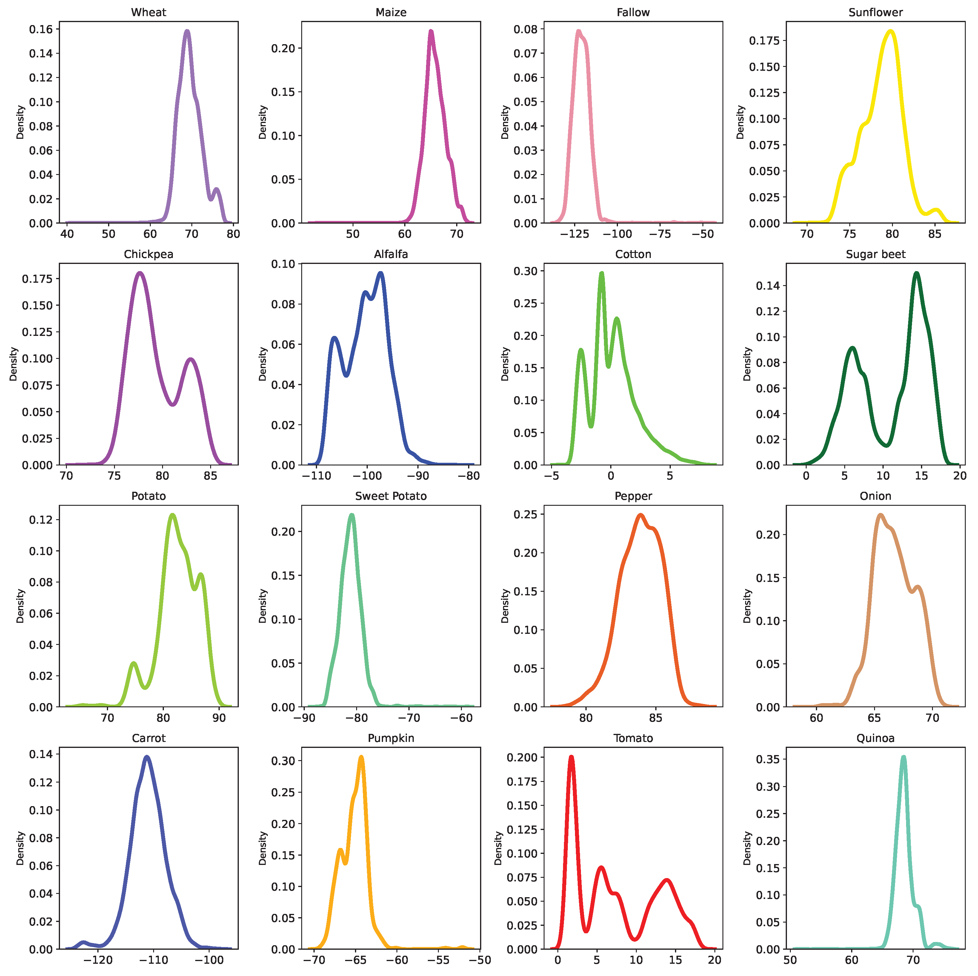
Now that we have validated our methodology quantitatively for the relabeling, using numerical criteria, we apply FARMSAR to the other half of the dataset and extract label errors and relabels. Then, we study the suggested relabels, and the detected mis-splits using optical imagery for qualitative validation of our method. A distribution of the embedding values of the class-expert CAEs used in this analysis are provided in Appendix A, but are not used in this study, as they do not offer a clear distinction of label anomalies.
5.1. Results
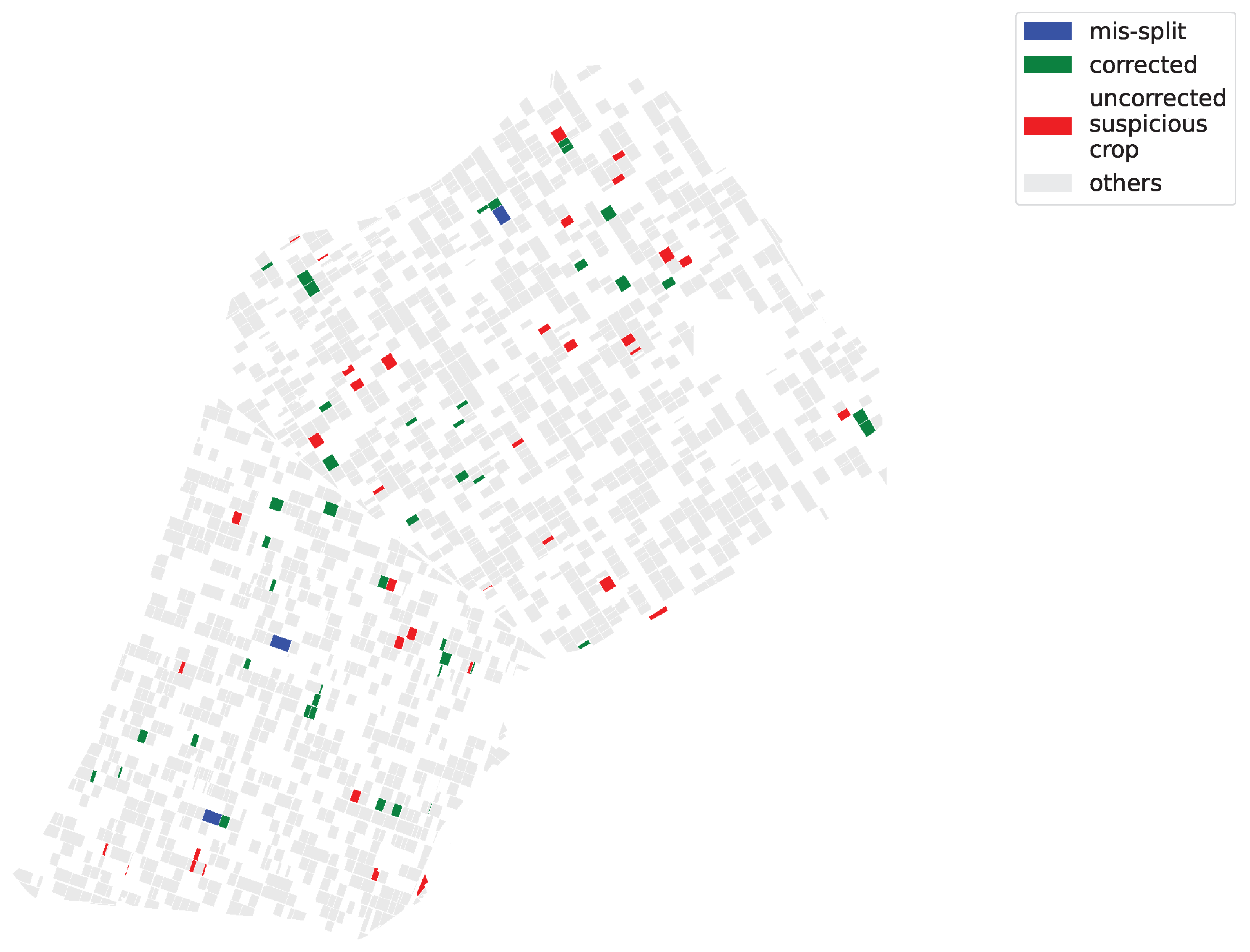
After applying the FARMSAR methodology to the second half of the dataset, left untouched and containing probable mislabels, we can extract suspicious crops, correct potential mislabels, and detect mis-split crops. At first, we isolate 40,000 suspicious time series, out of the approximately 600,000 that make up this half of the dataset. Then, according to Figure 13:
- FARMSAR discovers 3 mis-split crops;
- our method classifies 81 crops as suspicious mislabels (around 5% out of the approx. 1600 crops of this half of the dataset). FARMSAR relabels 44 crops confidently, and 37 crops are to be inspected for potential erroneous labels.
We also can observe in Figure 13a common pattern within the “suspicious” plots, corrected or not. Indeed, multiple of them appear side-by-side with one another. Considering that the labeling software of Sector BXII farmers is point-and-click, we assume that parts of the detected errors come from misclick manipulations, which swapped labels of two neighboring plots.
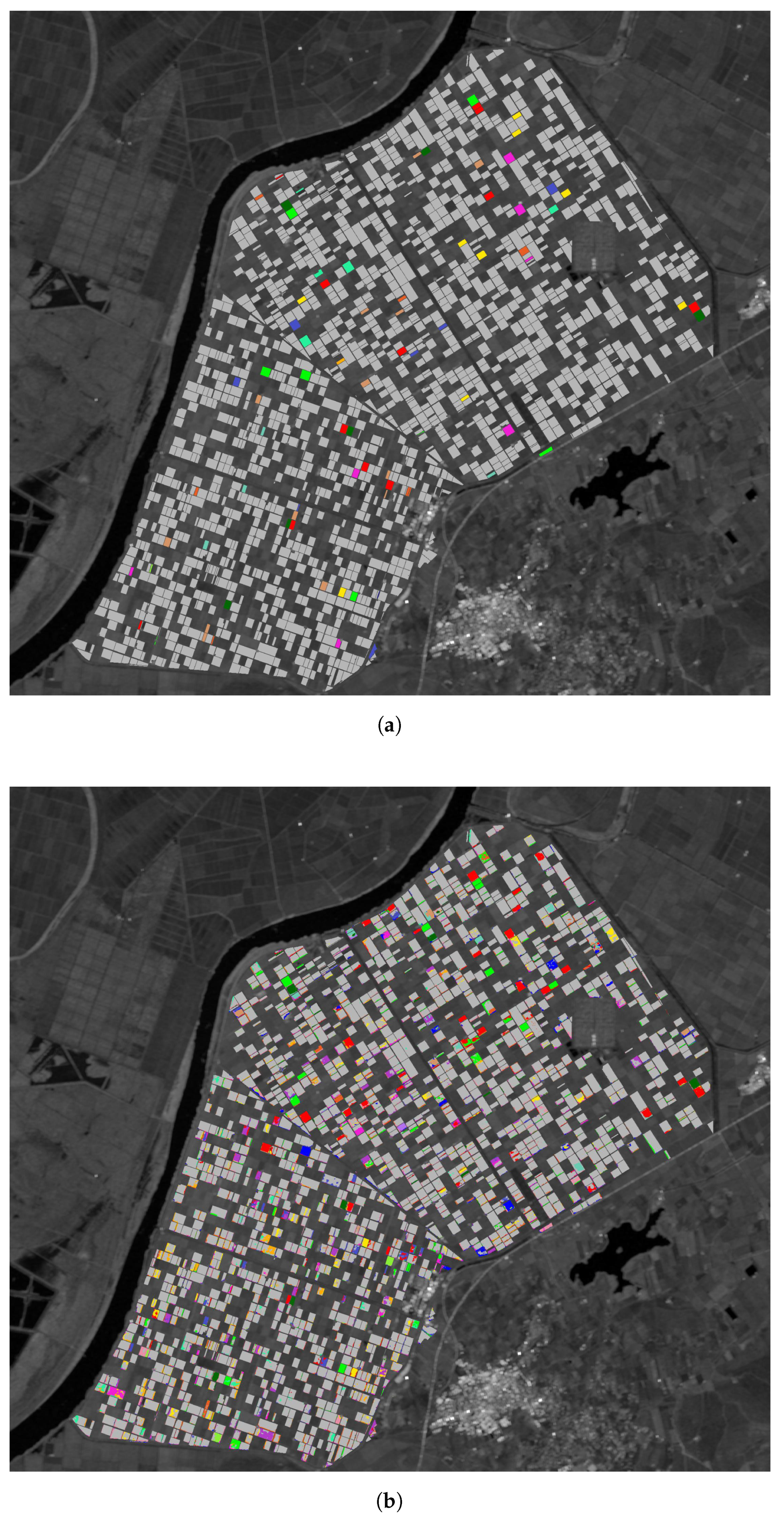
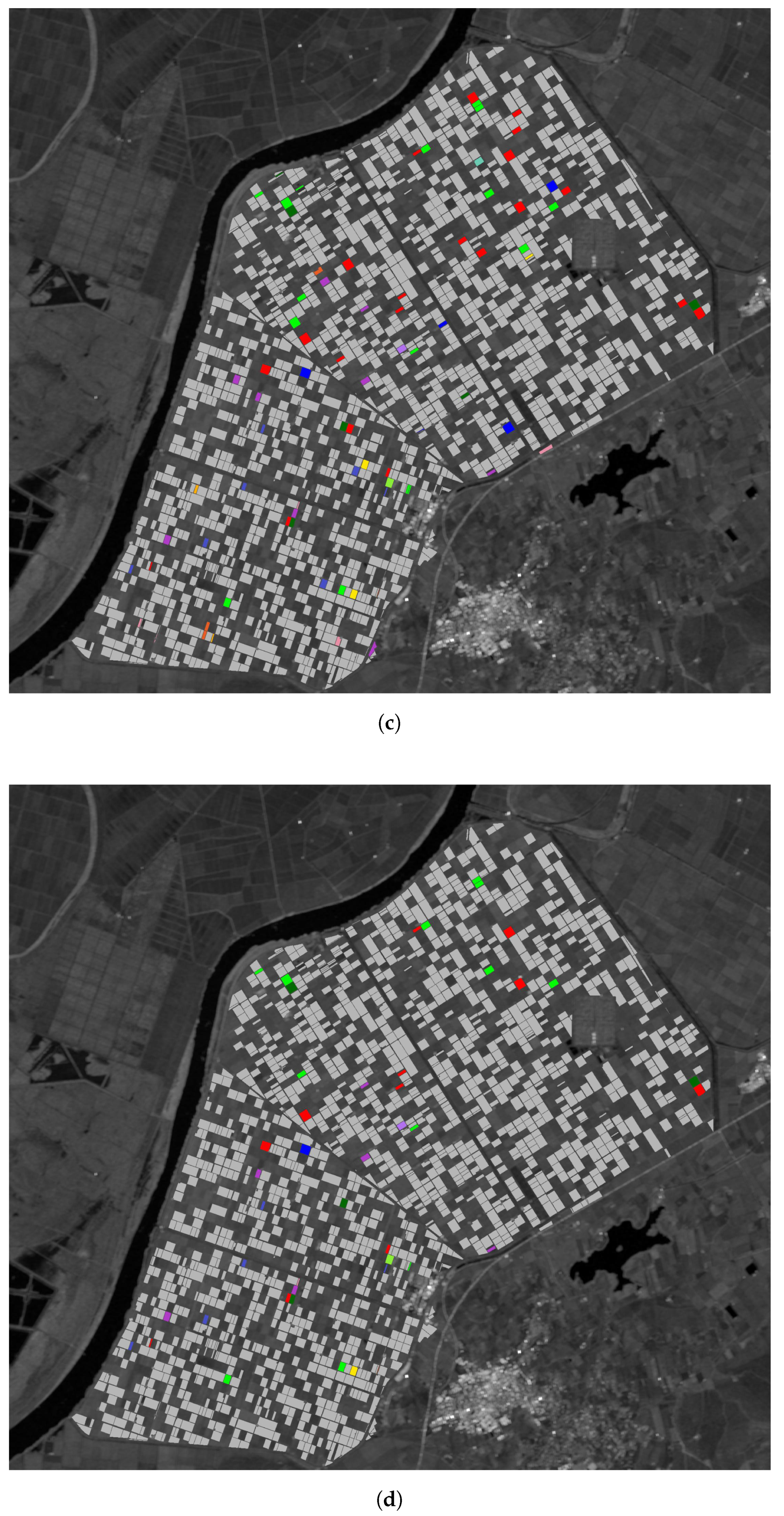
In Figure 14, we display a comparison between the corrected crops’ class before launching FARMSAR and after every step of the method. We can observe the presence of a variety of error types, as aforementioned: in Figure 14b, we notice the presence of edge cases but also heterogeneously relabeled crop. This relabeling noise justifies the shift toward a crop-level relabeling decision, as illustrated in Figure 14c. Nonetheless, given the proposed agricultural context, high confidence is required and thus restricts the number of final decisions regarding relabeling, as seen in the varying proportion of corrected crops between Figure 14c,d. However, as mentioned before, the suspicious crops are not discarded but set aside to be reinspected. Indeed, while the assignment of a new class is deemed inconclusive, the crop is still identified as an anomaly compared to the radiometric profiles of other crops of its class.
In addition, in Figure 14c,d, we observe the inversion of classes between juxtaposed crops, when compared to the ground truth displayed in Figure 14a. While not all instances of this phenomenon were confidently relabeled, four pairs of crops still got their labels inverted. This strengthens once more our original hypothesis regarding the probable origin of some of the detected mislabels: part of the mislabels come from click errors during the manipulation of the labeling software. Thus, the addition of a priori knowledge regarding common labeling mistakes could improve the relabeling decision by directing mislabel detection algorithms in a suggested direction or another.
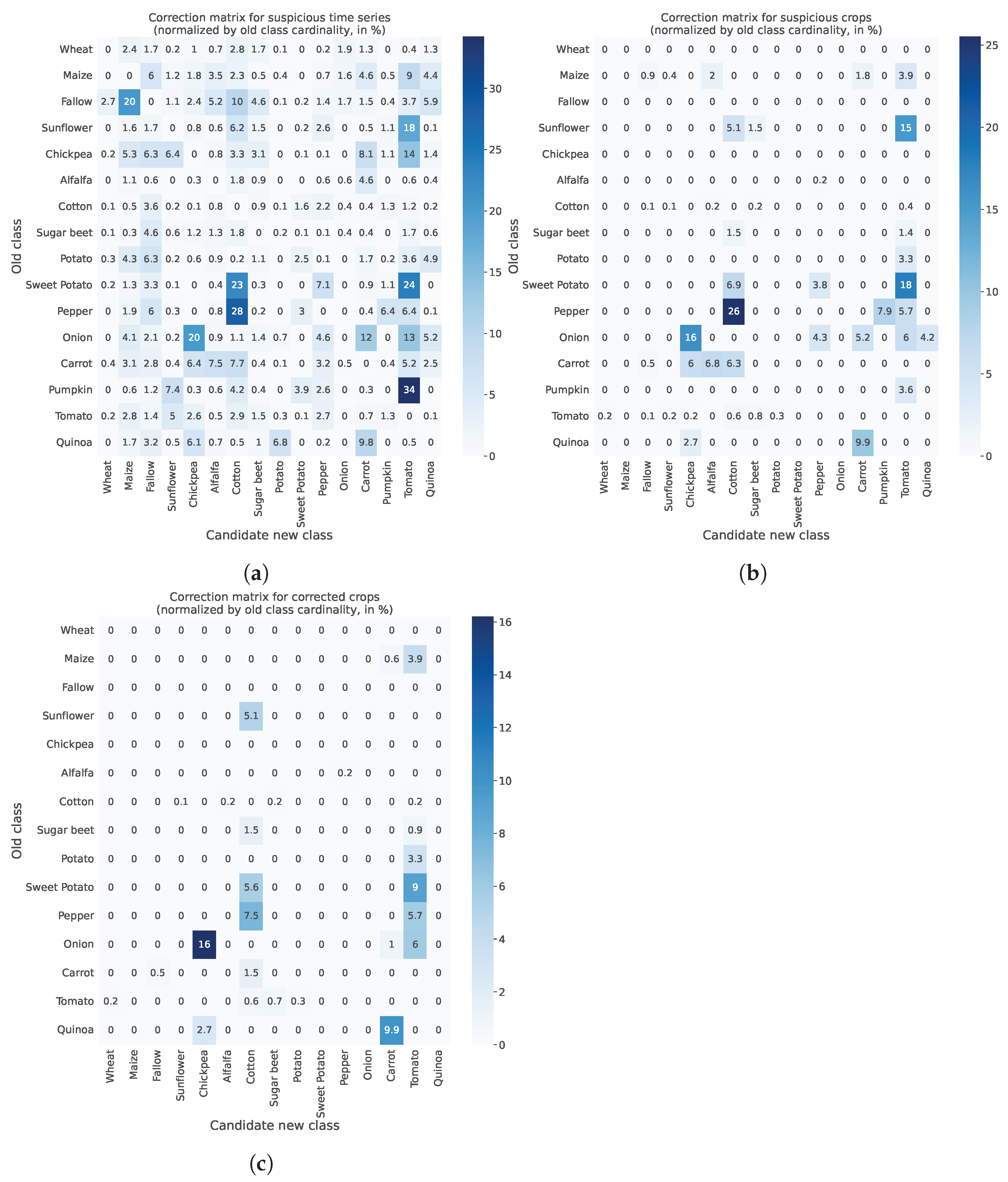
For numerical interpretation of the progressive filtering of candidate relabels performed by FARMSAR, we display in Figure 15 what we call relabeling matrices. We count, for each old class, how many time series are relabeled in a new class, and normalize it by the total amount of time series in the old class. We observe that candidate relabels at the first stage of the algorithm, in Figure 15a, are numerous: the reported confusions of small amplitude correspond to the aforementioned edge cases, illustrated in Figure 14b. They are removed at the second stage of the algorithm when turning to plot-level decision, as shown in Figure 15b. Finally, the ultimate confidence-based filtering reveals the relabels.
When analyzing relabels on a relative class per-class basis, they range from less than 1% for classes like Cotton to more than 20% for classes like Onion. We then highlight labeling mistakes that, taken in a global context, are in the minority but represent a significant portion of their crop type population. Thus, they must be addressed as decision-making on a crop type to crop type basis relies on the accurate indexing of crops. A percentage bias of more than two digits can critically impact the efficiency of decisions.
5.2. Qualitative Validation: Sentinel-2 Imagery over the First Group of Crops
The qualitative validation regards the validation of the results, presented in Section 5.1, using optical imagery to evaluate the credibility of relabeled crops and crops diagnosed as mis-splits.
5.2.1. Validation of Relabels
The validation of relabels involves a two-step process: validate that they are not of the supplied class, and that the new class is correct. We compare trustworthy plots of each class with mislabeled and relabeled plots of the same class, using Sentinel-2 imagery in visible light.
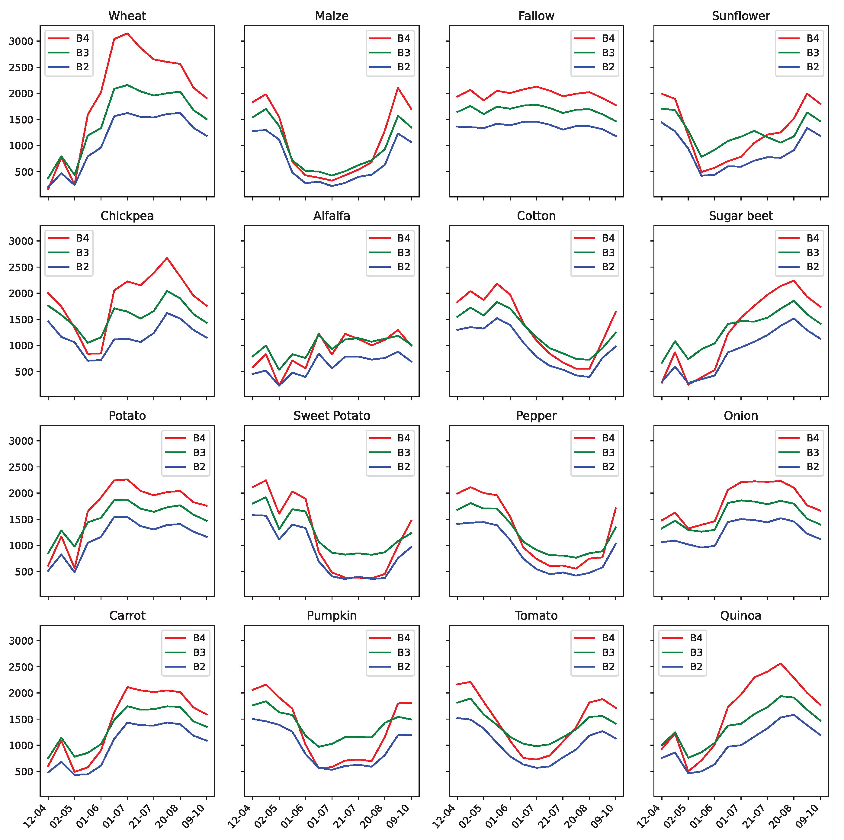
We display in Table 5 for a given class C a reference image of a trustworthy parcel, which we compare with the visual aspect of parcels that were mislabeled as C, and with parcels that were relabeled as C. If no field was mislabeled as C, or relabeled as C, we simply display the ∅ symbol. The majority of the detected mislabeled and proposed relabels can be corroborated using the available Sentinel-2 imagery. Some classes are still difficult to distinguish with optical imagery only: examples of such are the Pepper mislabels. When we compare, in Figure 16, the average temporal profiles of Sentinel-2 visible bands of the Pepper class to others, we highlight a high degree of similarities between peppers, sweet potatoes and cotton crops, for instance.
5.2.2. Validation of Mis-Splits
As mentioned above, we diagnosed three mis-split crops that we will independently validate, one by one, using Sentinel-2 imagery. To better understand the decision to label them as mis-split, we first compare a ground truth image of the plot’s class alongside an image where individual pixels correspond to their respective Sentinel-1 time series’ candidate class, according to their MSE vector. Then, we accompany it with Sentinel-2 images of each available timestamp over the observed region in 2017.
Mis-Split Field n°1
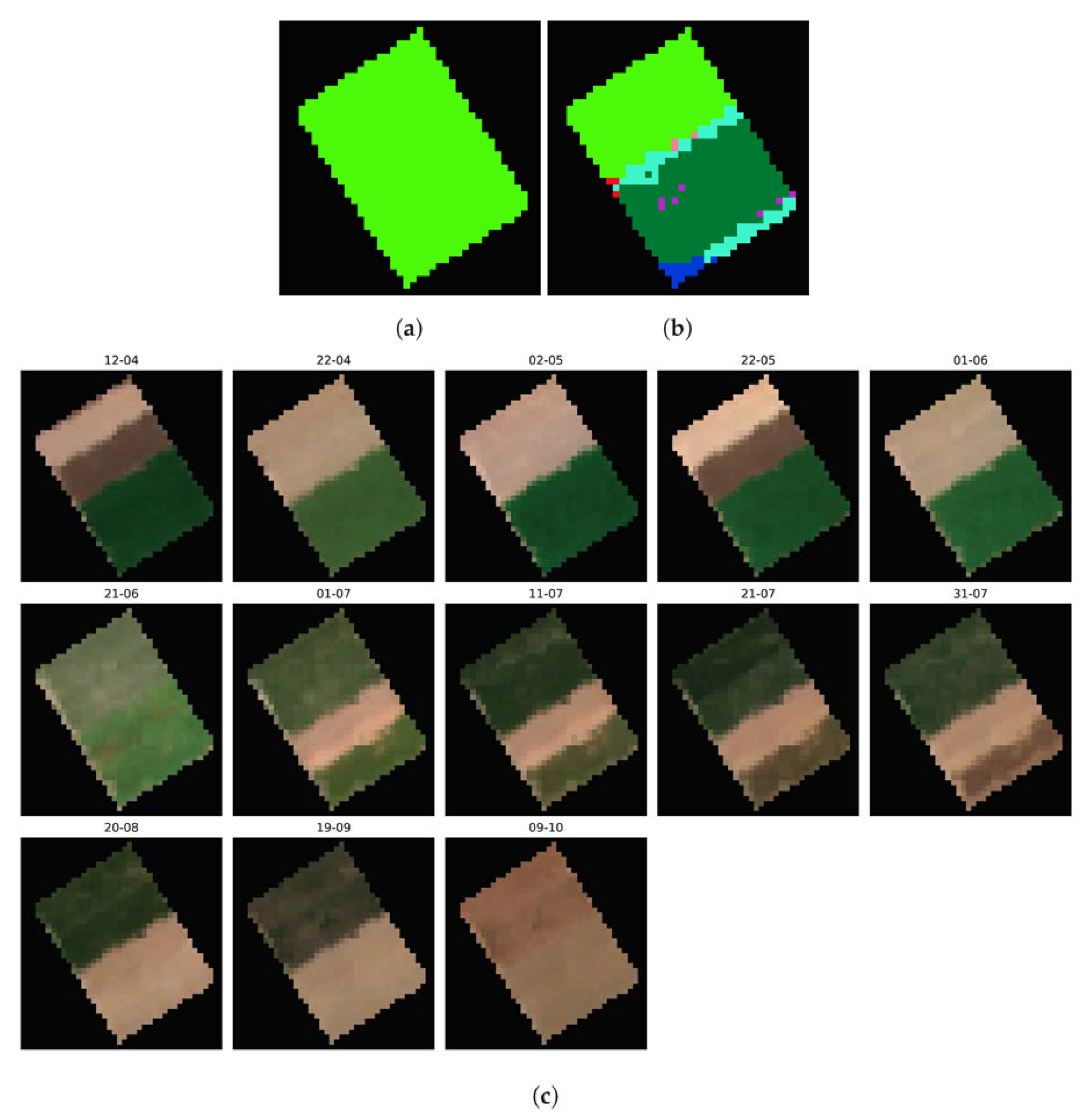
In Figure 17, we observe a clear split in two halves of the supposedly uniform crop: the first half, in light green, corresponds to cotton, while the second, in dark green, corresponds to Sugar Beets. The plot thus appears mis-split, according to our processing of Sentinel-1 time series. When turning to the optical analysis of the field’s evolution, shown in Figure 17c, we also observe an apparent separation between two halves of the crop, with a supposed cotton half of the field and a supposed sugar beet half. Each of them appears to be split even further in two, potentially resulting in four distinct crop types within a single field. Upon inspection of the radiometric temporal profile of each of these four, we establish that the visible differences in April for the Cotton half, and July for the Sugar Beets class, are linked to offset in harvest/seeding dates. Thus, taking into account the approximate growing period of sugar beets (December to May) and cotton (May to September), we can corroborate our method decision to relabel the top half as cotton, and the bottom half as sugar beets, when observing the Sentinel-2 images in Figure 17a.
Mis-Split Field n°2
In this second result, displayed in Figure 18, we observe once again a substantial distinction between the two halves of the crops, with the same presence of both sugar beets and cotton. In Figure 18c, the growth and harvest differences between the two halves of the crop make the mis-split condition of the crop very clear: the left half of the plot appears green during the growing season of beets, while the right half appears green during the growing season of cotton.
On a side note, we note in Figure 18b the presence of a third class, in light pink, which corresponds to fallow crops. When observing the Sentinel-2 images over the pixels labeled as fallow, some of them appear to be kept as bare ground (e.g., bottom-right of the plot). Thus, while the plot-level analysis is helpful in diagnosing plot-level anomalies, a time series-level analysis helps extract such insights, mostly linked to approximate labels and satellite imagery superposition.
Mis-Split Field n°3
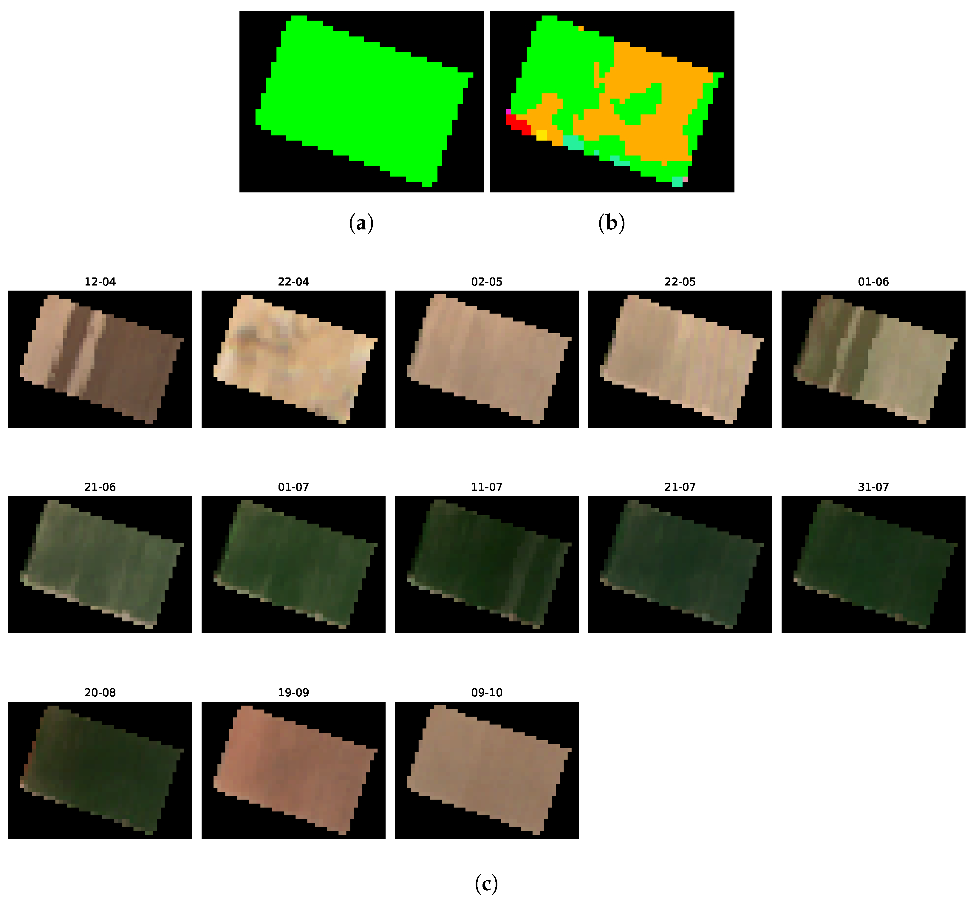
This third mis-split detection (Figure 19) is different than the last two we observed:
- the two classes that are potentially seen in the mis-split crop are “cotton” and “pumpkin”.
- the separation is not as clear as the last two mis-split crops.
In addition, when observing Figure 19c, we see a distinction between the two halves of the crop, but it appears much less apparent than for the other cases: a clear distinction regarding the ground conditions of the two halves can be observed in the images of the 12th of April and 1st of June. In this situation, the help of a field-expert to diagnose the reported mis-split is required.
6. Discussion
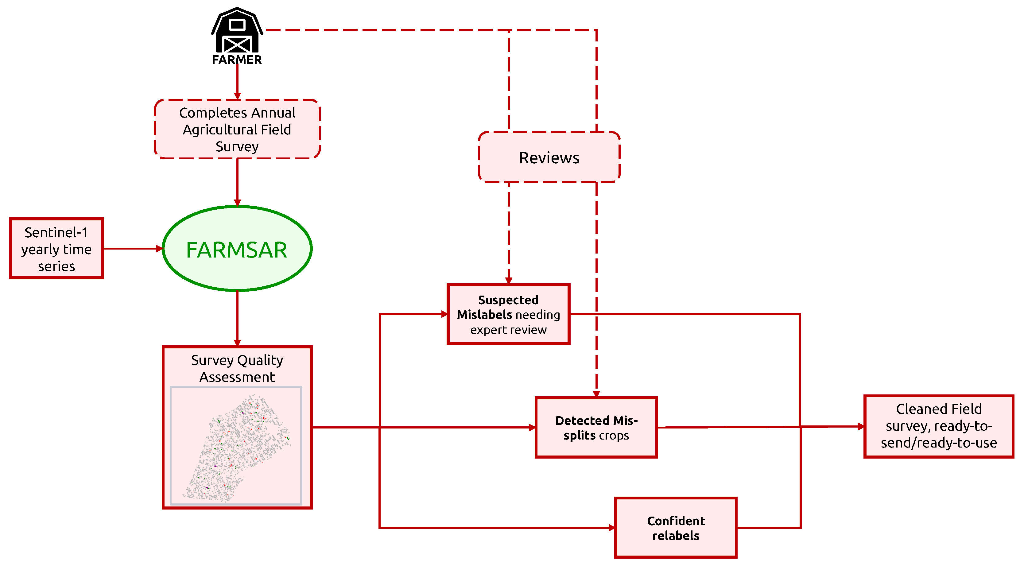
With its ability to extract a wide range of anomalies from field surveys, one of the potential applications of the presented methodology is its integration into farmers’ crop census process, as proposed in Figure 20. Indeed, various legal obligations regarding agricultural plots on a regional, national or international scale require a high-quality agricultural crop census for better big-picture monitoring of the farming performance by administrations. To further ensure this quality, providing farmers with automated tools that combine the latest advances in Remote Sensing and Artificial Intelligence can help tackle human mistakes, which could otherwise result in sanctions. However, such a tool should not introduce new errors under any circumstance. The action of relabeling must be subject to solid confidence criteria, which is embodied by the reconstruction error of our class-expert CAEs. In addition, we do not discard relabeling candidates that do not pass Otsu-based confidence criteria, but we label them as “uncorrected suspicious crops”. We can imagine providing the farmer with a candidate relabeling class for these suspicious crops. His final decision to relabel or remap crops builds on top of the FARMSAR methodology, making the whole process a sort of anomaly detection-guided double-check.
In this context, such a methodology can be useful for various administrative bodies:
- On a farmer’s side, FARMSAR provides a fast and reliable methodology to double-check the agricultural census of grown crops, leading to less risk-taking at the time of declaration.
- On the local administration side, FARMSAR provides a tool to monitor the quality of the delivered census. FARMSAR could facilitate the detection and extraction of anomalies in declarations.
As of today, our application of FARMSAR to Sector BXII is at a local scale. We consider the extraction of anomalies relative to a norm extracted on a per-farm basis. The application of FARMSAR to multiple farming environments, of different regions, at the same time has yet to be assessed. While it is suitable for regional and national-scale anomaly detection, mixing different farms, the expected diagnosis performance we present in this paper is not directly applicable. Indeed, the more diversity in farming strategies of crops, the harder it becomes to define the norm that is used to detect deviating crops. Hopefully, previous work involving the use of autoencoders and crops has already demonstrated their capacity to model intra-class variance of crops and variations in harvesting strategies effectively [41]. In this way, the use of autoencoders for this task is full of potential and to be further studied.
7. Conclusions
This work presents a methodology to diagnose the labeling quality of crop census and offer corrections of detected mislabels, using a confidence metric based on autoencoders reconstruction error and binary otsu thresholding. We show the potential of our methodology to identify mis-split crops and mislabels and correct them. We also consider in this paper a concrete use-case of this methodology if supplied to farmers performing field surveys. We assess the possibility of running this methodology after the farmer’s declaration to detect and eventually correct human labeling mistakes. In a context where farmers’ declarations are subject to strict regulations and can drive economic and ecologic decision-making, limiting the impact of mislabels on the said decisions is critical.
To conclude, in Angus et al. [32], the World Bank points out the “need for more suitable technologies” to support collaboration between “scientists, policymakers and farmers”. We believe FARMSAR is a step toward this collaborative direction.
Author Contributions
Conceptualization, T.D.M., R.G., L.T.-L. and E.C.; methodology, T.D.M.; software, T.D.M.; validation, T.D.M., R.G., L.T.-L. and E.C.; formal analysis, T.D.M., R.G., L.T.-L. and E.C.; investigation, T.D.M.; resources, T.D.M., R.G., L.T.-L. and E.C.; data curation, T.D.M.; writing—original draft preparation, T.D.M., R.G., L.T.-L. and E.C.; writing—review and editing, T.D.M., R.G., L.T.-L. and E.C.; visualization, T.D.M.; supervision, R.G., L.T.-L. and E.C. All authors have read and agreed to the published version of the manuscript.
Funding
This research received no external funding.
Institutional Review Board Statement
Not applicable.
Informed Consent Statement
Not applicable.
Data Availability Statement
Restrictions apply to the availability of these data. Data was obtained from Pr Juan M. Lopez-Sanchez, the correspondence to contact for its obtention.
Acknowledgments
The authors would like to thank Juan M. Lopez-Sanchez for providing us with the reference data originating from the Regional Government of Andalucía and the Spanish Agrarian Guarantee Fund (FEGA) and for the preprocessed multitemporal Sentinel-1 images. The authors would also like to thank him for the thoughtful scientific discussions. We also want to thank the reviewers for their feedback and help to improve the overall quality of this work.
Conflicts of Interest
The authors declare no conflict of interest.
Appendix A
Figure A1.
Density plots of each class 1D latent space after class-expert training for dataset correction, estimated using a kernel density estimate.
Figure A1.
Density plots of each class 1D latent space after class-expert training for dataset correction, estimated using a kernel density estimate.

References
- Kurosu, T.; Fujita, M.; Chiba, K. Monitoring of rice crop growth from space using the ERS-1 C-band SAR. IEEE Trans. Geosci. Remote Sens. 1995, 33, 1092–1096. [Google Scholar] [CrossRef]
- Le Toan, T.; Ribbes, F.; Wang, L.F.; Floury, N.; Ding, K.H.; Kong, J.A.; Fujita, M.; Kurosu, T. Rice crop mapping and monitoring using ERS-1 data based on experiment and modeling results. IEEE Trans. Geosci. Remote Sens. 1997, 35, 41–56. [Google Scholar] [CrossRef]
- Bhogapurapu, N.; Dey, S.; Bhattacharya, A.; Mandal, D.; Lopez-Sanchez, J.M.; McNairn, H.; López-Martínez, C.; Rao, Y. Dual-polarimetric descriptors from Sentinel-1 GRD SAR data for crop growth assessment. ISPRS J. Photogramm. Remote Sens. 2021, 178, 20–35. [Google Scholar] [CrossRef]
- Orynbaikyzy, A.; Gessner, U.; Mack, B.; Conrad, C. Crop Type Classification Using Fusion of Sentinel-1 and Sentinel-2 Data: Assessing the Impact of Feature Selection, Optical Data Availability, and Parcel Sizes on the Accuracies. Remote Sens. 2020, 12, 2779. [Google Scholar] [CrossRef]
- Mestre-Quereda, A.; Lopez-Sanchez, J.M.; Vicente-Guijalba, F.; Jacob, A.W.; Engdahl, M.E. Time-Series of Sentinel-1 Interferometric Coherence and Backscatter for Crop-Type Mapping. IEEE J. Sel. Top. Appl. Earth Obs. Remote Sens. 2020, 13, 4070–4084. [Google Scholar] [CrossRef]
- McNairn, H.; Champagne, C.; Shang, J.; Holmstrom, D.; Reichert, G. Integration of optical and Synthetic Aperture Radar (SAR) imagery for delivering operational annual crop inventories. ISPRS J. Photogramm. Remote Sens. 2009, 64, 434–449. [Google Scholar] [CrossRef]
- Jiao, X.; Kovacs, J.M.; Shang, J.; McNairn, H.; Walters, D.; Ma, B.; Geng, X. Object-oriented crop mapping and monitoring using multi-temporal polarimetric RADARSAT-2 data. ISPRS J. Photogramm. Remote Sens. 2014, 96, 38–46. [Google Scholar] [CrossRef]
- Hoekman, D.H.; Vissers, M.A.M.; Tran, T.N. Unsupervised Full-Polarimetric SAR Data Segmentation as a Tool for Classification of Agricultural Areas. IEEE J. Sel. Top. Appl. Earth Obs. Remote Sens. 2011, 4, 402–411. [Google Scholar] [CrossRef]
- Di Martino, T.; Guinvarc’h, R.; Thirion-Lefevre, L.; Koeniguer, E.C. Beets or Cotton? Blind Extraction of Fine Agricultural Classes Using a Convolutional Autoencoder Applied to Temporal SAR Signatures. IEEE Trans. Geosci. Remote Sens. 2022, 60, 1–18. [Google Scholar] [CrossRef]
- Dey, S.; Bhattacharya, A.; Ratha, D.; Mandal, D.; McNairn, H.; Lopez-Sanchez, J.M.; Rao, Y. Novel clustering schemes for full and compact polarimetric SAR data: An application for rice phenology characterization. ISPRS J. Photogramm. Remote Sens. 2020, 169, 135–151. [Google Scholar] [CrossRef]
- Adrian, J.; Sagan, V.; Maimaitijiang, M. Sentinel SAR-optical fusion for crop type mapping using deep learning and Google Earth Engine. ISPRS J. Photogramm. Remote Sens. 2021, 175, 215–235. [Google Scholar] [CrossRef]
- Ndikumana, E.; Ho Tong Minh, D.; Baghdadi, N.; Courault, D.; Hossard, L. Deep Recurrent Neural Network for Agricultural Classification using multitemporal SAR Sentinel-1 for Camargue, France. Remote Sens. 2018, 10, 1217. [Google Scholar] [CrossRef] [Green Version]
- Tiedeman, K.; Chamberlin, J.; Kosmowski, F.; Ayalew, H.; Sida, T.; Hijmans, R.J. Field Data Collection Methods Strongly Affect Satellite-Based Crop Yield Estimation. Remote Sens. 2022, 14, 1995. [Google Scholar] [CrossRef]
- Pelletier, C.; Valero, S.; Inglada, J.; Champion, N.; Marais Sicre, C.; Dedieu, G. Effect of Training Class Label Noise on Classification Performances for Land Cover Mapping with Satellite Image Time Series. Remote Sens. 2017, 9, 173. [Google Scholar] [CrossRef] [Green Version]
- Abay, K. Measurement Errors in Agricultural Data and their Implications on Marginal Returns to Modern Agricultural Inputs. Agric. Econ. 2020, 51, 323–341. [Google Scholar] [CrossRef] [Green Version]
- Zhong, J.X.; Li, N.; Kong, W.; Liu, S.; Li, T.H.; Li, G. Graph Convolutional Label Noise Cleaner: Train a Plug-And-Play Action Classifier for Anomaly Detection. In Proceedings of the IEEE/CVF Conference on Computer Vision and Pattern Recognition (CVPR), Long Beach, CA, USA, 15–20 June 2019. [Google Scholar]
- Aggarwal, C.C. An Introduction to Outlier Analysis. In Outlier Analysis; Springer International Publishing: Cham, Switzerland, 2017; pp. 1–34. [Google Scholar] [CrossRef]
- Enderlein, G.; Hawkins, D.M. Identification of Outliers. Biom. J. 1987, 29, 198. [Google Scholar] [CrossRef]
- Chalapathy, R.; Borzeshi, E.Z.; Piccardi, M. An Investigation of Recurrent Neural Architectures for Drug Name Recognition. arXiv 2016, arXiv:1609.07585. [Google Scholar] [CrossRef]
- Wulsin, D.; Blanco, J.A.; Mani, R.; Litt, B. Semi-Supervised Anomaly Detection for EEG Waveforms Using Deep Belief Nets. In Proceedings of the 2010 Ninth International Conference on Machine Learning and Applications, Washington, DC, USA, 12–14 December 2010; pp. 436–441. [Google Scholar]
- Song, H.; Jiang, Z.; Men, A.; Yang, B. A Hybrid Semi-Supervised Anomaly Detection Model for High-Dimensional Data. Comput. Intell. Neurosci. 2017, 2017, 1–9. [Google Scholar] [CrossRef] [Green Version]
- Gong, D.; Liu, L.; Le, V.; Saha, B.; Mansour, M.R.; Venkatesh, S.; Hengel, A.V.D. Memorizing Normality to Detect Anomaly: Memory-Augmented Deep Autoencoder for Unsupervised Anomaly Detection. In Proceedings of the IEEE/CVF International Conference on Computer Vision (ICCV), Seoul, Republic of Korea, 27 October–2 November 2019. [Google Scholar]
- Aytekin, C.; Ni, X.; Cricri, F.; Aksu, E. Clustering and Unsupervised Anomaly Detection with l2 Normalized Deep Auto-Encoder Representations. In Proceedings of the 2018 International Joint Conference on Neural Networks (IJCNN), Rio de Janeiro, Brazil, 8–13 July 2018; pp. 1–6. [Google Scholar] [CrossRef]
- Wang, N.; Li, B.; Xu, Q.; Wang, Y. Automatic Ship Detection in Optical Remote Sensing Images Based on Anomaly Detection and SPP-PCANet. Remote Sens. 2019, 11, 47. [Google Scholar] [CrossRef] [Green Version]
- Meroni, M.; Fasbender, D.; Rembold, F.; Atzberger, C.; Klisch, A. Near real-time vegetation anomaly detection with MODIS NDVI: Timeliness vs. accuracy and effect of anomaly computation options. Remote Sens. Environ. 2019, 221, 508–521. [Google Scholar] [CrossRef]
- León-López, K.M.; Mouret, F.; Arguello, H.; Tourneret, J.Y. Anomaly Detection and Classification in Multispectral Time Series Based on Hidden Markov Models. IEEE Trans. Geosci. Remote Sens. 2022, 60, 1–11. [Google Scholar] [CrossRef]
- Santos, L.A.; Ferreira, K.R.; Camara, G.; Picoli, M.C.; Simoes, R.E. Quality control and class noise reduction of satellite image time series. ISPRS J. Photogramm. Remote Sens. 2021, 177, 75–88. [Google Scholar] [CrossRef]
- Wang, C.; Shi, J.; Zhou, Y.; Li, L.; Yang, X.; Zhang, T.; Wei, S.; Zhang, X.; Tao, C. Label Noise Modeling and Correction via Loss Curve Fitting for SAR ATR. IEEE Trans. Geosci. Remote Sens. 2022, 60, 1–10. [Google Scholar] [CrossRef]
- Avolio, C.; Tricomi, A.; Zavagli, M.; De Vendictis, L.; Volpe, F.; Costantini, M. Automatic Detection of Anomalous Time Trends from Satellite Image Series to Support Agricultural Monitoring. In Proceedings of the 2021 IEEE International Geoscience and Remote Sensing Symposium IGARSS, Brussels, Belgium, 11–16 July 2021; pp. 6524–6527. [Google Scholar] [CrossRef]
- Crnojević, V.; Lugonja, P.; Brkljač, B.N.; Brunet, B. Classification of small agricultural fields using combined Landsat-8 and RapidEye imagery: Case study of northern Serbia. J. Appl. Remote Sens. 2014, 8, 083512. [Google Scholar] [CrossRef] [Green Version]
- Otsu, N. A Threshold Selection Method from Gray-Level Histograms. IEEE Trans. Syst. Man Cybern. 1979, 9, 62–66. [Google Scholar] [CrossRef] [Green Version]
- Angus, D.; Kernal, D.; William, E.; Takatoshi, I.; Joseph, S.; Shadid, Y. World Development Report 2008: Agriculture for Development; The World Bank: Washington, DC, USA, 2007. [Google Scholar] [CrossRef]
- Song, X.P.; Potapov, P.V.; Krylov, A.; King, L.; Di Bella, C.M.; Hudson, A.; Khan, A.; Adusei, B.; Stehman, S.V.; Hansen, M.C. National-scale soybean mapping and area estimation in the United States using medium resolution satellite imagery and field survey. Remote Sens. Environ. 2017, 190, 383–395. [Google Scholar] [CrossRef]
- D’Andrimont, R.; Verhegghen, A.; Lemoine, G.; Kempeneers, P.; Meroni, M.; van der Velde, M. From parcel to continental scale – A first European crop type map based on Sentinel-1 and LUCAS Copernicus in-situ observations. Remote Sens. Environ. 2021, 266, 112708. [Google Scholar] [CrossRef]
- Beegle, K.; Carletto, C.; Himelein, K. Reliability of recall in agricultural data. J. Dev. Econ. 2012, 98, 34–41. [Google Scholar] [CrossRef] [Green Version]
- Wollburg, P.; Tiberti, M.; Zezza, A. Recall length and measurement error in agricultural surveys. Food Policy 2021, 100, 102003. [Google Scholar] [CrossRef]
- Kilic, T.; Moylan, H.; Ilukor, J.; Mtengula, C.; Pangapanga-Phiri, I. Root for the tubers: Extended-harvest crop production and productivity measurement in surveys. Food Policy 2021, 102, 102033. [Google Scholar] [CrossRef]
- Gong, P.; Liu, H.; Zhang, M.; Li, C.; Wang, J.; Huang, H.; Clinton, N.; Ji, L.; Li, W.; Bai, Y.; et al. Stable classification with limited sample: Transferring a 30-m resolution sample set collected in 2015 to mapping 10-m resolution global land cover in 2017. Sci. Bull. 2019, 64, 370–373. [Google Scholar] [CrossRef]
- Lozano, D.; Arranja, C.; Rijo, M.; Mateos, L. Canal Control Alternatives in the Irrigation Distriction ’Sector BXII, Del Bajo Guadalquivir’, Spain. In Proceedings of the Fourth International Conference on Irrigation and Drainage, Sacramento, CA, USA, 3–6 October 2007; pp. 667–679. [Google Scholar]
- Clevert, D.A.; Unterthiner, T.; Hochreiter, S. Fast and accurate deep network learning by exponential linear units (elus). arXiv 2015, arXiv:1511.07289. [Google Scholar]
- Di Martino, T.; Koeniguer, E.C.; Thirion-Lefevre, L.; Guinvarc’h, R. Modelling of agricultural SAR Time Series using Convolutional Autoencoder for the extraction of harvesting practices of rice fields. In Proceedings of the EUSAR 2022; 14th European Conference on Synthetic Aperture Radar, Leipzig, Germany, 25–27 July 2022; pp. 1–6. [Google Scholar]
Figure 1.
Illustration of the BXII Sector (36°59 N 6°06 W) and reference crop types data over a Sentinel 1 VH polarization image acquired in orbit 74 on the 3rd of January 2017.
Figure 1.
Illustration of the BXII Sector (36°59 N 6°06 W) and reference crop types data over a Sentinel 1 VH polarization image acquired in orbit 74 on the 3rd of January 2017.

Figure 2.
Histogram of referenced crop types distribution (in number of fields).

Figure 3.
Visualization of an example of suspected mislabeled crops from the Sector BXII crop survey, with confusion between Cotton (green) and Sugar Beet (dark green) crops. (a) Superposition of Sentinel-2 RGB image of 22/04/17 and supplied crop types; (b) Sentinel-2 RGB image acquired the 22/04/17.

Figure 4.
Visualization of an example of a suspected mis-split Cotton crop from the Sector BXII crop survey. (a) Superposition of Sentinel-2 RGB image of 22/04/17 and supplied crop types; (b) Sentinel-2 RGB image acquired the 22/04/17.
Figure 4.
Visualization of an example of a suspected mis-split Cotton crop from the Sector BXII crop survey. (a) Superposition of Sentinel-2 RGB image of 22/04/17 and supplied crop types; (b) Sentinel-2 RGB image acquired the 22/04/17.

Figure 5.
Convolutional Autoencoders Architecture for the processing of sequential data, such as SAR time series.
Figure 5.
Convolutional Autoencoders Architecture for the processing of sequential data, such as SAR time series.

Figure 6.
Methodology for the detection of mis-split and mislabeled crops with a pixel-wise time series-level analysis at first, followed by a crop-level analysis.
Figure 6.
Methodology for the detection of mis-split and mislabeled crops with a pixel-wise time series-level analysis at first, followed by a crop-level analysis.

Figure 7.
Class-expert CAEs parallel training.

Figure 8.
Illustration of a vector of Mean-Squarred errors, used to identify suspicious and non-suspicious time series.
Figure 8.
Illustration of a vector of Mean-Squarred errors, used to identify suspicious and non-suspicious time series.

Figure 9.
Plot-Level rule-based classification of anomalies. Class color code is the same as in Figure 1.
Figure 9.
Plot-Level rule-based classification of anomalies. Class color code is the same as in Figure 1.

Figure 10.
Multiple applications of automatic binary Otsu Thresholding strategy to reconstruction histograms of class-specific time series. (a) Histogram of reconstruction error of onion-labeled S1 time series (blue), with Intra-class variance curve for different values of thresholds (orange) and optimal threshold (red). (b) Histogram of reconstruction error of sugar beet-labeled S1 time series (blue), with Intra-class variance curve for different values of thresholds (orange) and optimal threshold (red). (c) Histogram of reconstruction error of carrot-labeled S1 time series (blue), with Intra-class variance curve for different values of thresholds (orange) and optimal threshold (red).


Figure 11.
Trustworthy crops filtering process for Quantitative Validation.

Figure 12.
Performance measurements and comparison between our methodology and others (Vanilla CAE, Random Forests, Linear SVM). (a) Amount of corrected mislabels (eq. to recall measurement). (b) Amount of correct relabels (eq. to precision measurement).
Figure 12.
Performance measurements and comparison between our methodology and others (Vanilla CAE, Random Forests, Linear SVM). (a) Amount of corrected mislabels (eq. to recall measurement). (b) Amount of correct relabels (eq. to precision measurement).

Figure 13.
Maps of diagnosed Sector BXII crop fields.

Figure 14.
State of suspect crops and time series classes at every step of the method. Classes are displayed only for suspect crops/time series, for ease of visualization. Other crops are shown in gray. (a) Class image of suspect crops before relabeling. (b) Candidate class image of every suspicious time series (trustworthy time series in gray). (c) Candidate class image of every suspicious crops (no Otsu Thresholding applied). (d) Class image after relabeling (Otsu Thresholding applied).


Figure 15.
State of suspect crops and time series classes at every step of the method. Classes are displayed only for suspect crops/time series, for ease of visualization. Other crops are shown in gray. (a) Relabeling matrix at the first step of FARMSAR: time series relabeling (in percentage). (b) Relabeling matrix at the second step of FARMSAR: crop relabeling (in percentage) (no Otsu Thresholding applied). (c) Relabeling matrix at the second step of FARMSAR: crop relabeling (in percentage) (Otsu Thresholding applied).

Figure 16.
Average temporal profile, per available agricultural class, from Sentinel-2 visible light bands.
Figure 16.
Average temporal profile, per available agricultural class, from Sentinel-2 visible light bands.

Figure 17.
Comparison between the ground truth and candidate classes image of the first mis-split field, alongside multitemporal Sentinel-2 imagery of the parcel. (a) Ground truth class image of the mis-split field n°1. (b) Candidate classes image of the mis-split field n°1. (c) Sentinel-2 imagery of the first detected mis-split field.

Figure 18.
Comparison between the ground truth and candidate classes image of the second mis-split field, alongside multitemporal Sentinel-2 imagery of the parcel. (a) Ground truth class image of the mis-split field n°2. (b) Candidate classes image of the mis-split field n°2. (c) Sentinel-2 imagery of the second detected mis-split field.

Figure 19.
Comparison between the ground truth and candidate classes image of the second mis-split field, alongside multitemporal Sentinel-2 imagery of the parcel. (a) Ground truth class image of the mis-split field n°3. (b) Candidate classes image of the mis-split field n°3. (c) Sentinel-2 imagery of the third detected mis-split field.

Figure 20.
Suggested pipeline of usage of our methodology to support farmer’s field survey process.


Table 1.
Metadata of Sector BXII Sentinel-1 multitemporal stack.
| Sentinel-1 Acquisitions Metadata | |
|---|---|
| Acquisition Mode | Interferometric Wide |
| Polarisation | VV + VH |
| Relative Orbit Number | 74 |
| Wavelength | C-Band |
| Orbit Pass | Ascending |
| Near Incidence Angle | approx. 31.47° |
| Far Incidence Angle | approx. 32.82° |
| Acquisition Dates | 3 Jan. to 29 Dec. 2017 |
| Location | 36°59′00.0″ N 6°06′00.0″ W |
Table 2.
Architecture of the Convolutional Autoencoder used in this study.
| Operation Layer | Number of Filters | Size of Each Filter | Stride Value | Padding Value | Ouput Vector Size | |
|---|---|---|---|---|---|---|
| Input time series | - | - | - | - | ||
| Convolution Layer | 1D Convolution | 64 | 7 | 1 | 1 | |
| ELU | - | - | - | - | ||
| Pooling Layer | Max Pooling 1D | - | 2 | 2 | - | |
| Convolution Layer | 1D Convolution | 128 | 5 | 1 | 0 | |
| ELU | - | - | - | - | ||
| Pooling Layer | Max Pooling 1D | - | 2 | 2 | - | |
| Convolution Layer | 1D Convolution | 256 | 3 | 1 | 0 | |
| ELU | - | - | - | - | ||
| Pooling Layer | Max Pooling 1D | - | 2 | 2 | - | |
| Flatten Layer | Flatten | - | - | - | - | 1280 |
| FC Layer | Fully Connected | - | - | - | - | 128 |
| ELU | - | - | - | - | 128 | |
| FC Layer | Fully Connected | - | - | - | - | 64 |
| ELU | - | - | - | - | 64 | |
| FC Layer | Fully Connected | - | - | - | - | 32 |
| ELU | - | - | - | - | 32 | |
| Embedding Layer | Fully Connected | - | - | - | - | 1 |
| ELU | - | - | - | - | 1 | |
| FC Layer | Fully Connected | - | - | - | - | 32 |
| ELU | - | - | - | - | 32 | |
| FC Layer | Fully Connected | - | - | - | - | 64 |
| ELU | - | - | - | - | 64 | |
| FC Layer | Fully Connected | - | - | - | - | 128 |
| ELU | - | - | - | - | 128 | |
| Output Layer | Fully Connected | - | - | - | - | 122 |
| Reshape | - | - | - | - | ||
Table 3.
Training parameters for Class-expert CAEs.
| Method | Parameterization |
|---|---|
| CAE | ADAM optimizer |
| Learning Rate = 1 × 10 | |
| Batch Size = 128 | |
| Epochs = 20 |
Table 4.
Performance comparison between methodologies. (Best performance highlighted in bold).
| Mislabels’ Proportion | Amount of Corrected Mislabels | Amount of Correct Relabels | ||||||
|---|---|---|---|---|---|---|---|---|
| F-CAE 1 | CAE | SVM | RF | F-CAE 1 | CAE | SVM | RF | |
| 1 | 0.62 | 0.92 | 0.90 | 0.95 | 0.95 | 0.71 | 0.52 | 0.56 |
| 5 | 0.62 | 0.90 | 0.85 | 0.94 | 0.97 | 0.90 | 0.80 | 0.86 |
| 10 | 0.59 | 0.88 | 0.77 | 0.90 | 0.98 | 0.92 | 0.79 | 0.91 |
| 15 | 0.53 | 0.81 | 0.67 | 0.87 | 0.94 | 0.84 | 0.78 | 0.90 |
| 20 | 0.44 | 0.71 | 0.59 | 0.83 | 0.92 | 0.77 | 0.70 | 0.89 |
| 25 | 0.42 | 0.67 | 0.48 | 0.73 | 0.89 | 0.73 | 0.55 | 0.85 |
| 30 | 0.31 | 0.59 | 0.38 | 0.60 | 0.86 | 0.71 | 0.49 | 0.77 |
1 Otsu-Filtered CAE, our methodology.
Table 5.
Visual validation of mislabels and relabels with Sentinel-2 Imagery.
| Class | S2 Date (DD/MM/YYYY) | True ... | Mislabeled as ... | Relabeled as ... |
|---|---|---|---|---|
| Alfalfa | 12/04 |  |  |  |
| 11/07 |  |  |  | |
| Carrot | 22/05 |  |  |  |
| 21/07 |  |  |  | |
| Chickpea | 12/04 |  | ∅ |  |
| 01/06 |  | ∅ |  | |
| Cotton | 01/06 |  |  |  |
| 20/08 |  |  |  | |
| Fallow | 12/04 |  | ∅ |  |
| 21/06 |  | ∅ |  | |
| Maize | 12/04 |  |  | ∅ |
| 21/06 |  |  | ∅ | |
| Onion | 12/04 |  |  | ∅ |
| 21/06 |  |  | ∅ | |
| Pepper | 12/04 |  |  |  |
| 20/08 |  |  |  | |
| Potato | 12/04 |  |  |  |
| 20/08 |  |  |  | |
| Quinoa | 12/04 |  |  | ∅ |
| 21/06 |  |  | ∅ | |
| Sugar Beet | 22/05 |  |  |  |
| 20/08 |  |  |  | |
| Sunflower | 12/04 |  |  | ∅ |
| 01/06 |  |  | ∅ | |
| Sweet Potato | 21/06 |  |  | ∅ |
| 30/08 |  |  | ∅ | |
| Tomato | 12/04 |  |  |  |
| 21/06 |  |  |  | |
| Wheat | 22/05 |  | ∅ |  |
| 01/06 |  | ∅ |  |
Disclaimer/Publisher’s Note: The statements, opinions and data contained in all publications are solely those of the individual author(s) and contributor(s) and not of MDPI and/or the editor(s). MDPI and/or the editor(s) disclaim responsibility for any injury to people or property resulting from any ideas, methods, instructions or products referred to in the content. |
© 2022 by the authors. Licensee MDPI, Basel, Switzerland. This article is an open access article distributed under the terms and conditions of the Creative Commons Attribution (CC BY) license (https://creativecommons.org/licenses/by/4.0/).
Share and Cite
MDPI and ACS Style
Di Martino, T.; Guinvarc’h, R.; Thirion-Lefevre, L.; Colin, E. FARMSAR: Fixing AgRicultural Mislabels Using Sentinel-1 Time Series and AutoencodeRs. Remote Sens. 2023, 15, 35. https://0-doi-org.brum.beds.ac.uk/10.3390/rs15010035
AMA Style
Di Martino T, Guinvarc’h R, Thirion-Lefevre L, Colin E. FARMSAR: Fixing AgRicultural Mislabels Using Sentinel-1 Time Series and AutoencodeRs. Remote Sensing. 2023; 15(1):35. https://0-doi-org.brum.beds.ac.uk/10.3390/rs15010035
Chicago/Turabian StyleDi Martino, Thomas, Régis Guinvarc’h, Laetitia Thirion-Lefevre, and Elise Colin. 2023. "FARMSAR: Fixing AgRicultural Mislabels Using Sentinel-1 Time Series and AutoencodeRs" Remote Sensing 15, no. 1: 35. https://0-doi-org.brum.beds.ac.uk/10.3390/rs15010035
Note that from the first issue of 2016, this journal uses article numbers instead of page numbers. See further details here.