Article

A New Approach to Estimate Fuel Budget and Wildfire Hazard Assessment in Commercial Plantations Using Drone-Based Photogrammetry and Image Analysis

School of Science Technology and Engineering, University of the Sunshine Coast, Sippy Downs 4556, Australia
*
Author to whom correspondence should be addressed.
Remote Sens. 2023, 15(10), 2621; https://0-doi-org.brum.beds.ac.uk/10.3390/rs15102621
Submission received: 18 April 2023 / Revised: 12 May 2023 / Accepted: 16 May 2023 / Published: 18 May 2023
(This article belongs to the Special Issue Earth Observation and UAV Applications in Forestry)

Abstract

:
Increased demand for sustainable timber products has resulted in large investments in agroforestry in Australia, with plantations growing various Pinus species, selected to suit a plantation’s environment. Juvenile Pinus species have a low fire tolerance. With Australia’s history of wildfires and the likelihood of climate change exacerbating that risk, the potential for a total loss of invested capital is high unless cost-effective targeted risk minimisation is part of forest management plans. Based on the belief that the understory profiles within the juvenile plantations are a major factor determining fuel hazard risks, an accurate assessment of these profiles is required to effectively mitigate those risks. At present, assessment protocols are largely reliant on ground-based observations, which are labour-intensive, time consuming, and expensive. This research project investigates the effectiveness of using geospatial analysis of drone-derived photographic data collected in the commercial pine plantations of south-eastern Queensland as a cost-saving alternative to current fuel hazard risk assessment practices. Understory composition was determined using the supervised classification of orthomosaic images together with derivations of canopy height models (CHMs). The CHMs were subjected to marker-controlled watershed segmentation (MCWS) analysis, isolating and removing the plantation pine trees, enabling the quantification of understory fuel profiles. The method used proved highly applicable to immature forest environments with minimal canopy closure, but became less reliable for close canopied older plantations.

1. Introduction

An expanding human population has driven increased demand for timber products, placing stress on supply and threatening the survival of native forest resources [1,2]. In response, the agroforestry industry has expanded to meet the growing commercial demand for a plantation product that is deemed to be sustainable and the result of responsible environmental practices [3,4]. In south-east Queensland, plantation trees can take up to 25 years to reach commercial maturity [5], and consequently, large amounts of capital are invested in an agricultural industry that is slow to produce returns on investment. During this time, the crop faces a myriad of potential threats including drought, floods, pests and fire, any of which could lead to a total loss of monies invested [6]. Therefore, responsible forest management practice needs to include strategies designed to mitigate a total loss of invested funds. With respect to fire, risk mitigation needs to be based on a detailed knowledge of the location and structure of available fuels [7] and on an informed understanding of which components of those fuels represent the major risk, before resources tasked with reducing that risk can be effectively deployed.
The creation of fire requires three basic ingredients: a supply of suitable fuel, available oxygen and an ignition source. In an outdoor environment, the limitation of available oxygen is not feasible. Therefore, reducing the risk of a fire is limited to either eliminating the ignition source or reducing the amount of available dry fuel. Wildfire ignition sources can broadly be classified as either natural or anthropogenic [8]. Human behaviour concerning fire is often quite unpredictable and impossible to comprehend, with many fires resulting from deliberate acts of arson [9,10]. Despite this, lightning remains the largest source of natural ignitions [8,11]. However, after researching the causes of wildfires in south-eastern Australia, Nampak et al. [12] found that the percentage of strikes that result in an ignition event is extremely low, with an annual efficiency of only 0.24%. However, the study also concluded that low-level vegetation such as dry summer grasses and understories significantly increased the likelihood of a successful lightning ignition. This finding supports the assumption that lower-level vegetation is an important determinant of potential fire risk and further reinforces the belief that if the potential risk from a wildfire is to be mitigated, those tasked with performing the mitigation need a good understanding of the profiles of that lower-level vegetation, which, in many cases, is a forest or woodland understory.
Understanding the mechanisms of lightning and successful wildfire ignitions has been further complicated by a changing climate [8,13,14]. There is evidence that global warming has driven increased lightning activity and the logical conclusion is that this will result in more wildfires [15]. However, as weather events and atmospheric activity are outside anthropogenic control [11], the only risk mitigation pathway available is to improve methods of limiting the spread of fire following an ignition by reducing or altering the fuels available to support that spread.
Globally, forest ecosystems and ignition sources may vary, but few fires successfully increase in size without the existence of an understory with a volume, structure and sufficiently low moisture content capable of supporting that increase [16,17]. As with oxygen availability and ignition sources, the fuel moisture content usually cannot be feasibly altered in forested environments and, therefore, reductions in the development of a wildfire from an ignition revolve around interventions that reduce the understory fuel volumes or alter their structures before conditions favourable to the development of a wildfire exist.
Anthropogenic behaviour has altered forest understory composition and structure [4]. For example, land use changes in the Mediterranean have led to an increased amount of more flammable scrubby understory vegetation, increasing chances of ignition and fire intensity [18]. The situation has been further complicated by human-induced changes in climate patterns and associated increased periods of warmer weather, limiting the time available to implement planned fuel hazard reductions, and further contributing to potential scenarios of larger, more prevalent wildfires. Evidence suggests that this is already occurring in Australia, where the number and scale of wildfires have increased due to increased amounts of drier fuel resulting from longer, hotter seasons [19,20,21,22]. Similar conditions are emerging in Asia and the Americas as extended drier and hotter summer seasons produce increased volumes of dry understory fuels [23,24]. Most recent studies have concluded that this trend will continue [14,25].
Cruz et al. [26] concluded that high surface fuel loads were the primary factors influencing the ignition and spread of the intense 2009 Black Saturday Fires in Victoria, Australia. The surface fuels of concern were the dry understory layers comprising desiccated vegetation and remnant eucalypt litter such as bark and limbs [27,28]. Research by Erni et al. [29] supported the belief that understory profiles in the Canadian and North American forests were major determinants of fire ignition and spread.
Consequently, there is an increased need for intervention to reduce the risk of intense wildfires developing from ignition events occurring during fire-favourable weather conditions by reducing the available ground-level fuels [30,31]. Fuel load reductions primarily using controlled hazard reduction burns have long been used as the primary method of mitigating this risk [32,33], but in commercial forestry, fuel load management can also be in the form of chemical or mechanical reduction [5,34]. Fuel reduction burns to reduce the amount of available understory fuel by burning during the cooler seasons, with the aim being to reduce understory volume and alter the understory structure without damaging the tree crowns of taller vegetation. However, in some juvenile pine plantations, the use of fire can lead to tree mortality and is therefore not appropriate. Whatever the chosen method, effective fuel hazard reduction programmes direct what are usually limited resources towards regions assessed as being at substantial risk. Unless the ignition source of a forest fire is a fully developed crowning fire spreading from an adjacent forested environment, the initial ignition site and, consequently, the area of highest risk is likely to be in regions with dense understory vegetation, which becomes highly flammable as it dries [31]. Therefore, the effective implementation of hazard reduction requires a detailed assessment and a good understanding of that understory if effective measures are to be implemented to limit the likelihood of a successful ignition and subsequent spread [35]. At present, the assessment of sometimes large regions to determine potential high-risk locations within is largely based on field observations, which are both time-consuming and expensive. The reality of large capital losses due to increases in wildfire intensity and frequency has provided the impetus to improving forest management practices aimed at limiting the potential losses from destructive events.
Research projects have examined alternative methods that remotely sense forest structures. However, most of the early studies utilised data from satellite imagery, high-resolution aerial photographs or LiDAR, obtained using rotary or fixed-wing aircraft, to produce profiles of forest environments [7,36,37]. These methods were able to cover large areas, but were expensive to implement and the limited resolution of satellite imagery made the definition of smaller trees difficult [37,38,39]. The methodologies mainly concentrated on quantitative assessment of potential commercial timber inventories using Individual Tree Crown Detection and Delineation (ITCD) techniques [37,38].
The finer-scale analysis of forest environments has been enhanced by recent developments in unmanned aerial vehicle (UAV) photogrammetry and LiDAR, leading to the availability of more cost-effective options for forest structure profiling [37]. The higher resolution data, when compared to that of satellites, has enabled improved assessment of areas composed of smaller trees. Again, most of the initial studies concentrated on the quantification of commercial products contained beneath the forest canopy [37,38,39]. Despite extensive literature reviews conducted by the authors, it appears that to date, little work has been carried out using these techniques to determine what constitutes other forest layers such as the qualification and quantification of understory profiles as part of overall fuel hazard management planning.
Improvements in UAVs, the associated data sensing equipment payload and the computer software capable of analysing the resultant data have enabled some studies to extend profiling to include the complete forest environment. More recently, with an increased realisation of the fire risk associated with the forest floor and understory, there has been an emerging emphasis on the use of remote sensing technologies to profile the lower levels of forests [40,41].
The adaptation of remote sensing to improve efficiencies in fuel hazard management has potential benefits for not only the natural environment, but also agricultural operations, where loss due to fire has major financial implications [42]. This is especially relevant in (but not limited to) Australia, a country with a history of destructive wildfires that are likely to become more severe as climate change progresses. Of particular concern to this study is the growing potentially negative impacts on agricultural operations, particularly silviculture.
Research projects have attempted to find more economically viable methods to implement fire management protocols in forest environments around the world [43,44,45]. Many of those projects have investigated the use of UAV-supported remote sensing techniques [37,46]. Despite this research, the commercial pine industry has persisted in reliance on field observations to assess potential fire risks and to direct treatments. These methods are labour-intensive and therefore expensive [47]. This study aimed to investigate the use of drone-derived data using photogrammetry to determine the amount, composition and structure of understory fuels that could potentially improve efficiencies in fuel hazard management in the commercial pine plantations of south-eastern Queensland.

2. Materials and Methods

2.1. Overview

The aim of this study was to develop a simple, accurate method of using fuel load information from high-resolution drone-based RGB images and photogrammetry to determine the amount and types of understory vegetation in the plantation, with the secondary aim being to determine the composition of that understory from a fire risk perspective. Three field samples from three quadrats within each of the ten sites were collected in August and November 2020 using the same data collection, collation and assessment protocols. The data collected included maximum vegetation height, average vegetation height and a summary of vegetation composition within each sampling quadrat. Each site was surveyed using drone-based images that were processed for the creation of RGB orthomosaics and subjected to digital photogrammetry to derive dense point clouds (DPCs) of the surface elevation related to each location. Canopy height models (CHMs), understory vegetation height models (DSM(Un)s) and digital elevation models (DEMs) were generated using varying combinations of image, photogrammetry and geospatial analysis in the digital environment. Sunshine Coast Council (SCC) LiDAR data (2018) was used to verify the accuracy of the resultant DEMs. Fuel types were classified into four classes: bare ground (including pine needle debris), grasses/herbs/sedges/ferns/small shrubs (GHSFSS), residual debris (Litter) and woody weeds (WW) by applying ENVI Supervised Classification Workflows to RGB orthomosaics. The resultant fuel height and composition models were compared with the field samples obtained.

2.2. Specifics

2.2.1. Study Site Location

The study site locations were within the Hancock Queensland Plantations Pty Ltd. (HQP) Beerburrum Forest and located to the east of the Bruce Highway, approximately 55 km north of Brisbane (Figure 1). The plantation consisted of ‘Southern Pine’ species (Pinus caribaea and Pinus elliotti) and the 10 study sites selected ranged from new plantings to mature trees. HQP refers to individual plantation sites as ‘compartments’. The compartments chosen had a tree age range of 1–10 years. The compartment understory profiles comprised various combinations of grasses, mainly whisky grass (Andropogon virginicus), blady grass (Imperata cylindrica) and signal grass (Urochloa decumbens), sedges, shrubs, herbaceous species, bracken fern and dry remnant woody material. The area has an average annual precipitation of 1057 mm and an average temperature of 20.2 °C [48].

2.2.2. Field Data Collection

The compartments were all located within an area of 11 km2, with the study compartments ranging from 1.0 to 6.7 ha. For this study, the juvenile plantings were divided into three age groupings: Group A, trees 1–3 years of age (YOA); Group B, trees 4–7 YOA; and Group C, trees 8–10 YOA (Figure 1 and Table 1). The compartments were selected to reflect variations within each grouping.
Three sampling locations were randomly selected within each compartment as follows: From a point 20 m from the compartment boundary, the first predetermined compass bearing selected from a list generated using ‘Random Lists’ (https://www.randomlists.com/random-direction, accessed on 15 May 2023) was followed for a tape-measured distance of 50 m to sampling point one. A labelled stake (Group ID, Compartment Number and Site Number) was placed at the closest point within the planting row and the GNSS position was noted on the Field Survey Data Sheet using the GDA94 Zone 56 UTM Coordinate System. A 0.5 × 0.5 m quadrat was positioned one metre east of the stake (Figure 2). The maximum and average vegetation heights, a vegetation class summary and % ground cover within the quadrat were recorded.
From sampling location one, the next randomly selected bearing was followed for 50 m to sampling location 2, and the procedure was repeated for sampling location 3. Where a proposed sampling location was less than 10 m from the compartment border, a return was made to the previous sampling location and the next compass bearing selected.
This sampling process was performed twice, initially in August 2020 and later in November 2020. The protocols for both samplings were as previously described with the exception that in November, the sampling quadrats were positioned 1 m to the west of the positioned stake, whereas the quadrats were positioned 1 m to the east of the same stakes in August.

2.2.3. Drone-Based Image Collection

Colour composite images with red, green and blue bands were collected in November 2020 using a Phantom 4 Pro drone with a 4K camera, flown in a Double-Grid ‘PIX4D Capture’ pattern, at an altitude of 60 m AGL, with a 65° camera angle and 80% lateral and longitudinal image overlap. The spectral ranges of the red, green and blue bands are detailed in Appendix A. Flights were carried out in accordance with CASA regulations for the safe operation of an unmanned aerial vehicle (UAV) and by suitably qualified personnel in clear weather conditions with maximum winds not exceeding 20 kph.
The photographic data were stored on a 32 GB Micro SD card installed on the drone and uploaded to the computer system for further analysis.

2.2.4. Data Analysis

The data analysis workflow followed the pathway summarised by the eight steps below:
  • Orthomosaic generation;
  • DSM generation (through point cloud);
  • Identification of ground locations on orthomosaic to generate DEM from DSM;
  • CHM generation using the following algebraic expression in ArcGIS: CHM = DSM − DEM;
  • Calibration of above-ground height from objects with known heights (Figure 3). For this, the parked vehicles with known heights were used. Since there was not much difference between the estimated and actual height, no statistical tests and corrections to CHM were performed;
  • MCWS identification and elimination of plantation pine from CHM to create DSM(Un);
  • Classification of orthomosaic using RGB bands to determine understory composition;
  • Volume calculation using statistics from step 7.
The primary task was to generate high-quality dense point clouds (DPC) from the remotely sensed overlapping drone imagery. After some experimentation with Agisoft Metashape (1.7.1), Meshroom (2019.2.0), ArcGIS (10.6.1) and ArcGIS Pro (2.3.3), it was concluded that Agisoft Metashape produced the best results. Due to the data bank size and the calculations involved, batch processing was performed using Agisoft’s workflow and the university’s network processing facility.
The outcome was a series of high-resolution DPCs representing the vegetation three-dimensional shape profiles of each compartment A1–C3. Further processing of the DPCs resulted in high-resolution RGB composite orthomosaics for each compartment, including statistics relating to output resolution and accuracy. Initially, the project planned to use corrected GNSS positions of ground control points (GCPs) to georeference the computer-generated DPCs. For this investigation, horizontal accuracy, though important, was considered not as crucial as the accuracy of vertical measurements (i.e., vegetation height), and initially, the vehicle for acquiring that accuracy was the use of GCPs and corrected GNSS location coordinates to the georeference output. However, it quickly became apparent that this approach did not fit particularly well with the other aim of this study, which was to develop an efficient and simple system. The positioning and retrieval of GCPs is labour intensive and time consuming. Recording GNSS positions and correcting those positions consumes more time and further complicates the process, potentially increasing costs. In addition, for compartments greater than five years old, the method proved somewhat ineffective, as GCPs placed within the compartment area were often obscured from view and therefore not clear in the remotely sensed imagery. The practice of placement along the perimeter of a compartment defeated the purpose of GCP placement as their effective positioning required an even pattern of distribution within the area under survey. In this application, the need for very high accuracy was not crucial and therefore alternative methods of analysing the remotely sensed imagery without the use of GCPs were investigated.
To achieve this outcome, bare ground points were identified and selected on each orthomosaic RGB composite raster. Elevation values were extracted from the associated DSM and interpolated to produce a DEM. The contouring of the resultant DEM raster was checked for accuracy against the DEM produced from 2018 LiDAR point cloud data provided by the SCC.
The understory digital surface model (DSM(Un)) is a DSM of the forest understory and can be described as the CHM without the inclusion of the commercial plantation product. To identify and eliminate the unwanted component of the CHM, marker-controlled watershed segmentation (MCWS) algorithms were used. The process revolves around image reconstruction using a set of morphological filters to eliminate undesirable or unwanted features without affecting the remaining desired features [49] and, until now, has been used for the interpretation of medical imagery. Using ‘Forest Tools’ from the R Library [50], the MCWS algorithms were able to separate the understory profiles from other taller forest vegetation. This was achieved by subjecting the reference image, the orthomosaic of the compartment, to an algorithm that morphologically reconstructed the image, eliminating the taller plantation pine trees to reveal the remaining understory height profiles. The output model was the DSM(Un) for that compartment. The position of each pixel within the DSM(Un) raster was that pixel’s x and y value and the colouration or greyscale intensity, dependent on the selected symbology, represented the z value or the understory vegetation height associated with that pixel.
In addition to the vegetation height measurements, the field data included data summarising the vegetation type and the percentages of each located within the quadrats sampled. The intention was to compare these data with the vegetation composition modelling resulting from the computer classification of the ‘RGB composite’ orthomosaics of each compartment. The classification was performed using ENVI V5.6 (64-bit) software. The chosen classification workflow was that of supervised classification (maximum likelihood algorithm) with data training for 5 classes (bare ground, grasses/herbs/sedges/ferns/small shrubs (GHSFSS), larger woody weeds (non-pine species > 1.5 m tall) (WW) and debris (Litter)). The training criterion employed was a minimum of fifteen training polygons per class for each compartment that were drawn for homogeneous areas around locations collected in the field. To determine the understory composition, unclassified (UnC°) and pine (P°) percentages were eliminated and the resultant percentages of bare ground, GHSFSS, WW and Litter were calculated using the formula below:
% U n d e r s t o r y G H S F S S = 100   ×   G H S F S S ° 100 U n C ° + P °
where GHSFSS° is the percentage of grasses/herbs/sedges/ferns/small shrubs in the supervised classification class statistics, and UnC° and are the percentages of the unclassified and pine components of those same statistics. The detail of field data about specific vegetation types was more extensive than that possible by computer classification modelling. For the purposes of comparison, the field data divisions were refined into the same five classes as the supervised classification models; bare ground including pine needle cover, grasses/herbs/sedges/ferns/small shrubs (GHSFSS), residual debris (Litter) and larger woody weeds (WW). ArcGIS zonal statistics relating to the classified composition model ‘tif’ rasters included the average height of vegetation classes and the percentage cover of the classes in each compartment. Using these values, the calculation of the volumes of each vegetation class within a compartment was possible, completing the process of understory composition profiling.

2.2.5. Statistical Analysis

The resultant fuel height and composition models were compared with the field samples obtained and the strength of the correlations was tested using MS Excel statistical data analysis software (MS Excel version 2301). The correlations between field-measured data and the modelled data were tested using the Pearson correlation test and reported according to statistical analysis best practice.

3. Results

3.1. Field Data Summary of Compartment Vegetation Composition and Heights

The compartments were initially selected to reflect the variability in the understory structure, composition and their overall commercial development. The compartments demonstrated diverse species composition (Appendix B and Figure 4) and there was also variation in the plantation tree height ranges between compartments of similar age. For example, in Compartment B3, the trees had not reached the same height as those in the other same-aged compartments B1 and B3. Growth in C3 had surpassed C1 and C2.
It is evident from Figure 4 that as the compartment age and canopy closure advance, there are generally increased amounts of woody shrubs, lantana and sedges. The observed fuel load peaked in ‘B’ compartments (4–7 YOA) and then reduced.
The diversity in plant composition was also evident between compartments of the same age grouping. Figure 5, a comparison of the vegetation composition between compartments A1, A2, A3 and A4, graphically illustrates this high degree of variability. This variation was also reflected in the compositional structures within the ‘B’ and ‘C’ compartments. The species variability influenced the wide range of maximum and average heights within compartments and between compartments of similar age ranges.

3.2. GIS Data Analysis

3.2.1. Derived Products—Dense Point Clouds, Orthomosaics, Digital Surface Models and Digital Elevation Models

Dense point cloud and orthomosaic composites with red, green and blue bands were generated from the photographic data collected by the drone. This facilitated the creation of data products such as DSMs, DEMs, classified images, colourised point clouds and estimations of the composition of understory vegetation types including their areas and volumes. The raster data products generated were of a very high spatial resolution with ground sampling distances (GSD) of 1.67 cm. The clouds for all ‘A’ compartments and for B2 and B3 were extremely good and of a quality evident in Figure 6.
Several compartments (e.g., B1, C1, C2 and C3) exhibited areas without elevation points. These locations of ‘no data’ are evident in the DPC of compartment C1 shown in Figure 7. The orthomosaics generated from the DPCs of affected compartments exhibited some blurring in these affected areas. This phenomenon is likely attributable to the effects of vegetation movement due to wind. These areas were masked for CHM calculations, but were retained for compartment understory vegetation type classification.
Segments of the final RGB composite orthomosaic outputs are visually presented in Figure 8. The orthomosaics exhibit high levels of data quality for all compartments except for C1, where some blurring is evident in the centre left of the image.

3.2.2. CHMs Derivation and MCWS Analysis

(i) Canopy Height Models
The panel below (Figure 9) presents the results of the generation of CHM for each compartment. The plantation pine can be easily identified based on the patterns generated by the CHM. Additionally, the raster provides information about the height distribution of the understory vegetation.
(ii) MCWS Application and DSM(Un) Modelling
The application of the MCWS algorithm to the CHMs facilitated the isolation and removal of areas occupied by the taller pine vegetation (Figure 10). The remaining raster layer, the understory digital surface model (DSM(Un)), enabled the visualisation of the understory vegetation height distribution within each compartment (Figure 11). The white regions are areas of taller vegetation not perceived as understory and are therefore regions of ‘No Data’.
(iii) Understory Vegetation Heights and Statistical Analysis of the Results
The average height values of the compartment understories, extracted from the statistical summaries related to each of the DSM(Un) rasters, are summarised in Table 2. The range of difference in the numerical height values between the field samples and MCWS models varied from 0.2 cm (A2) to 21.5 cm (B3), but the biggest discrepancy occurred for C3, where the field sample average height was 15.7 cm, whereas the modelling produced an understory height average of 1 cm, a difference of 1470%.
The graphical representation of the field and modelled understory heights generally indicates that the modelling tended to predict lower values than was measured in the field, with the exceptions being B2 and C2. The difference between the field samples and the modelled values tended to increase with the plantation age groupings. For example, except for A4, where the difference between the field and modelled values was 17 cm, ‘A’ compartment values showed more correlation than was exhibited in the older B3 and the ‘C’ compartments.
Statistically, the field data and DSM(Un) results showed moderate support for an association between the two sets of values with a Pearson’s correlation coefficient (r) of 0.64, degrees of freedom = 8, p-value = 0.005 (Figure 12).

3.3. Vegetation Classification Model

The classified vegetation modelling for orthomosaics A1–C3 is illustrated in Figure 13. The comparison of the compartment composition field data and classified models is presented in Table 3. The presence of woody weeds in B2–C2 and the increased canopy cover in the ‘C’ compartments are evident.
The classified models and field observations showed close agreement for most ‘A’ and ‘B’ compartments. Both Figure 14a,b illustrate similarities in the trending of variations in the amounts of particular vegetation types in different compartments. For example, as evident in Figure 14a, the field data and the classifications agreed that there is less GHSFSS and bare ground in A2 when compared to A1 and the amount of bare ground was less in both A3 and A4 than in compartments A1 and A2. Whilst these trends and evidence of agreement continued with the ‘B’ compartments, an examination of Figure 14b suggests that the associations between the field data and the classified vegetation profiles became less convincing. For instance, in B1, both the field and modelled results agreed that there was a predominance of litter and the values for bare ground were similar. This scenario continued for B2, but the results for compartment B3 showed increasing divergence.
This move towards less agreement continued with the C1, C2 and C3 comparisons. The classification of C1 produced a value of 17.6% for woody weeds, whereas the field data supported an amount of 0.2%. In C2, the disagreement regarding the amount of woody weeds was also apparent, with a difference in the perceived values of 20.9%, and for C3, the classification yielded the presence of 1.1% bare ground, whereas none was evident in the field as the compartment was covered by a layer of pine needle debris. There was a large discrepancy between the amounts of litter and understory vegetation between the two sets of values for C3. These variations between the field and modelled values are graphically summarised in Figure 14c.
The statistical analysis of the relationships between the field and modelled values is summarised in Table 4. The results demonstrated that the correlations between the understory vegetation composition profiles observed in the field and the classification of the orthomosaic were very strong for compartments with minimal canopy closure, namely, the ‘A’ and ‘B’ compartments. The Pearson correlation coefficients (r values) were above 0.93, and p-values were less than 0.001, indicating a better than 99% chance of the existence of a very strong correlation between each of the two sets of values.
As the compartment canopy closure increased in the ‘C’ compartments, the strength of the associations decreased, with r values decreasing to 0.64, but the significance of this result was still greater than 0.05. This result is still encouraging and provides credible support for agreement between the field observations and the classified models of these more mature compartments.
The r values for all C compartments indicated weak correlations between the field results and the classified vegetation composition profiles, supported by low probabilities of an association, especially in compartments C2 and C3, where the p-values approached 0.5.

3.4. Understory Volumetric Calculations

The zonal statistics extracted from ArcGIS about the area, average vegetation heights and calculated total volumes of each vegetation class within the compartments are presented in Appendix C. The results have been expanded to include the volume per hectare. Accurate field values were not recorded, so the statistical significance of these values was not tested. However, the results are mostly consistent with general observations, with the exceptions being the amount of pine tree volume in B3 and the disparity between the amounts of low vegetation and litter in C3.

4. Discussion

This study successfully used drone-derived data to determine the amount, composition and structure of understory fuels that could potentially improve efficiencies in fuel hazard management forests. The goal was to develop a workflow that is efficient, cost-effective and of sufficient accuracy to safely direct fuel management protocols within the juvenile forest environment. The investigation concluded that the use of remotely sensed data to quantify understories was possible using the application of MCWS algorithms to identify and eliminate taller vegetation in the digital models, and with some further refinement, this method could become an alternative to the less efficient practices currently employed. The use of the supervised classification of orthomosaics successfully provided information about understory vegetation composition with a level of detail suitable for potential fuel hazard determination.
However, while the results were encouraging, certain aspects of this study indicate that further investigation and refinement would be required before this approach could become a viable commercial reality. The method showed very promising results for younger plantations where the understory was not obscured by canopy closure. This finding was consistent with many other remote sensing forest profiling studies where the results using photogrammetry were good in open forest environments, but became less accurate compared to LiDAR-based studies as forests aged [47,51,52].
In general, the use of MCWS to mask the commercial plantation trees for the subsequent modelling for average understory height calculations produced reliable results for less mature plantations—those 1–3 YOA and for some compartments 3–7 YOA. However, the outcomes for A4, B2 and B3 were exceptions. Despite the numerical variation in some more mature compartments, the trends were mostly consistent and statistically, the results were significant.
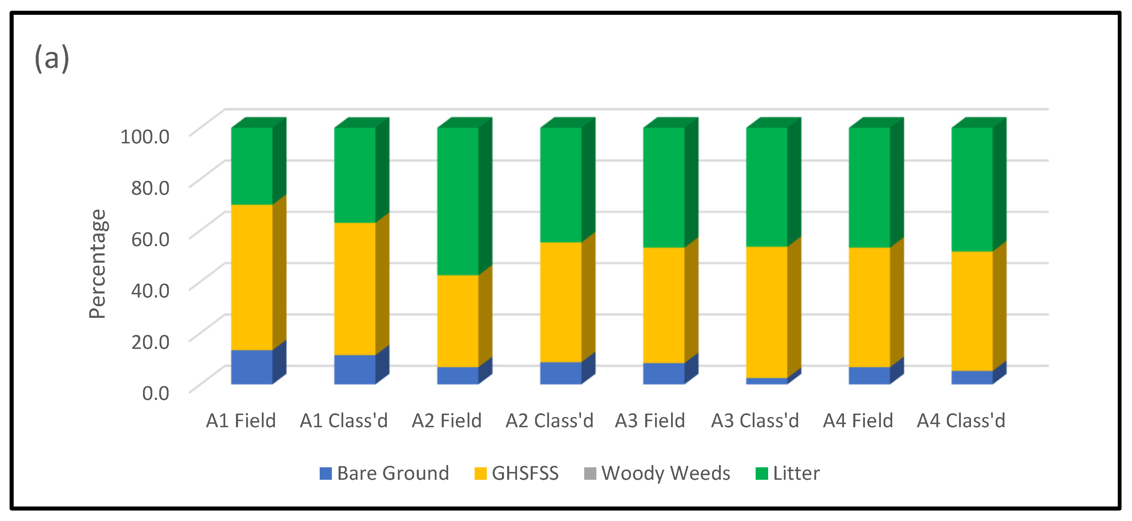
The classification results showed a similar pattern, with mostly good correlations in younger plantations and less agreement in those that were more mature, as canopy closure advanced limiting the detail of the aerial imagery. The statistical significance for the ‘A’ and ‘B’ compartments suggests a 99% chance that the results were correct and the correlations between the field and classified values were strong. The gap between the actual understory composition and the classified model widened with the ‘C’ compartments, where the results showed weaker agreement. As with the height calculations, this trend was probably due to a decrease in the percentage of visible understory within compartments as the amount of canopy closure increased.
The degree of error was potentially magnified in the more mature compartments as the classified composition model became increasingly based on smaller areas of visible vegetation, further contributing to a general deterioration in the results in older compartments. This explained the reasonably strong association between the two sets of average height values in the A compartments and B1, and the lessening of correlations in compartments B2, B3 and all C compartments where plantation maturity and increased canopy closure influenced the agreement between the field values and the analytical results. In these older compartments, the models produced were based on the limited areas within a compartment where the imagery included the understory. Our methods then expanded those findings to cover the invisible areas under the canopy, based on the assumption that the vegetation under the canopy layer had the same characteristics. Factors such as altered pH, shading and ground wetness may have affected the nature of the under-canopy vegetation [53] and the modelling assuming continuity may be flawed. The problems profiling understory in forests with advanced canopy closure might be overcome with the use of aerial LiDAR together with RGB cameras. Ongoing improvements in drone and LiDAR technologies are likely to make this a viable future alternative, but at the current level of development, drone-based systems capable of the necessary endurance whilst supporting a payload of both LiDAR equipment and an RGB camera is a more expensive option [54,55].
Successful height analysis using the remotely sensed data was hindered by the difficulty of establishing an effective ground zero. The drone was flown at 60 m above the ground height at the take-off/landing point. An idiosyncrasy of DJI Phantom 4 drones was that this did not necessarily mean that the image EXIF values relating to the altitude at which an image was taken corresponded to that value. Other studies using the same equipment have experienced similar problems [56]. The range variation in ground level altitude across all of the compartments was less than 4 m, whilst the range in EXIF values for the images obtained from the field flights was approximately 41.1 m (28.2 m (C2)–69.3 m (B2)). GNSS ‘georeferencing’ would usually be the method of choice used to correct these inconsistencies, but for the reasons previously alluded to, this study aimed to find methodologies that did not utilise this technique. Many alternative methods were trialled, and some did produce results. The reporting of those results was outside the scope of this study, but the researchers wondered whether some of those methods discarded due to lower correlations may have shown more promise if compared to the results emanating from a study with more field sampling.
A repetition of this study with an increased number of field data sampling sites per compartment would also influence correlation probabilities. The low number of samples affected the results in two ways. Firstly, it potentially altered the statistical analysis, elevating the critical values required for the results to have statistical significance. In several compartments, a favourable Pearson’s correlation coefficient was not supported by a correspondingly favourable statistical significance value. Secondly, it is possible that the field sampling was not extensive enough to reflect the true height or composition profiles of the compartments. The field observations indicated that large variations existed within compartments and between compartments of the same age grouping. Establishing understory average heights and composition within compartments using only six field samples was probably not an effective method of establishing an average height or composition profile reflective of that compartment, especially with respect to compartments with advanced canopy closure where the composition and structure of the understory became more complicated. An interesting result is that of compartment C3; this compartment had, at some time, been subjected to fire, possibly a fuel hazard reduction burn and the understory consisted of a small amount of remnant pine debris, some regenerated sedges and a continuous layer of pine needle litter approximately 100 mm in depth. The DSM(Un) resulted from MCWS application to a CHM derived using a DEM interpolated from ground points that may have potentially been the surface of the litter layer as captured in the drone imagery of compartment C3. Adjustment for this possible error would have significantly improved the results for the modelled average heights in this compartment. Similar potential error scenarios may have existed in other B and C compartments where shadowing and difficulties in the differentiation between the colour of bare ground and ground litter increased, complicating the determination of the true nature of the surface selected as a ground point. As before, point clouds produced from the analysis of aerial-derived LiDAR data would improve the results by minimising these errors.
The potential for the use of MCWS in the natural environment is only just being realised. As previously mentioned, it improves the delineation or outline of features of interest, enabling more accurate quantification of that feature. Initially, its main use was the interpretation of medical imagery such as MIRs to determine the extent of tumorous lesions. For example, the technology was investigated as a method to analyse imagery of human brains by Michael [57]. Cui et al. [58] were able to adapt MCWS to successfully interpret cancerous lesions in medical imagery of breast tissue. However, it has the potential to assist the interpretation of any form of imagery, and since 2010, its use has expanded to other fields including agriculture and industry. Devi and Singh [59] successfully used the algorithm to count pigs, and Heltin Genitha et al. [60] were able to use MCWS to delineate ships detected in satellite imagery. Dahlstrom et al. [61] adapted the use of MCWS to improve coating processes in paper manufacture. The forestry industry has recognised the benefits of applying MCWS to the delineation of individual tree canopies visible in aerial imagery [62,63,64]. However, after extensive literature searches, it is the author’s conclusion that this study is the first to investigate the use of MCWS algorithms to profile forest understories. Part of the initial goal for this project was to develop simple methods of data analysis. Complicated computer pathways involving highly developed software and large capacity hardware requires increased operator specialisation and drives increased costs [65]. In silviculture, the increased processing time from data acquisition to model availability decreases efficiency, elevates costs and possibly leads to the lack of outcome relevancy, as a forest is a constantly changing environment and opportunities may have been lost. Processing using ESRI software and subsequent MCWS application was complicated, and initial attempts involved using ArcGIS Pro to process the Agisoft Metashape DPC. Driven by a need to further understand the processes attempted and to refine those processes to improve results, the researchers reverted to using ArcGIS software, which allowed more operator input to refine the methodology. Once refined, processing could be simplified by producing workflows capable of completing the analysis more efficiently and without the need for continual analyst intervention.

5. Conclusions

This study demonstrates an alternative, more cost-effective method than direct field observations to determine fuel management in commercial as well as natural forest systems. Our research concluded that point cloud and orthomosaics resulting from the photogrammetric analysis of drone imagery and the subsequent derivation of canopy height models from that dense point cloud, the classification of the RGB orthomosaics and the application of MCWS on the CHMs could profile the understory vegetation within commercial pine plantations. With further refinement, the application of marker-controlled watershed segmentation to this method of understory vegetation modelling using remotely sensed UAV photographic imagery could become a very cost-effective and efficient method of understory fuel load determination, not only for use in these pine plantations, but in all forests where canopy closure does not inhibit views of most of the forest floor. However, in forests approaching levels of canopy maturity, this approach would have limited application in determining the amount of understory present, and the effective determination of that understory’s composition and structure using classification software would also be compromised.
Refinements in methodology might include further testing to fine-tune the MCWS parameters, enhancing the quality of the outcomes. Incorporating these upgrades into developed automated workflows would further improve efficiencies by reducing the amount of operator input required to complete the data analysis. Methodologies improving the ground point selection process, as part of DEM creation, would lead to improved accuracies in the calculation of the average understory vegetation heights.
Our results have been partially successful, indicating that alternative methods do exist and they do work in immature plantations. Considering that compartments of juvenile pine trees are the most susceptible to total investment loss in the event of even a mild wildfire, the method proposed and tested in this study is worthy of further consideration. The method is very cheap. It is quick and of high accuracy in immature forest plantings. The method could act as a stopgap until developments in UAV—LiDAR-RBG Camera platforms become a more commercially viable option.

Author Contributions

Conceptualisation, K.P., T.L. and S.K.S.; methodology, K.P.; software, S.K.S.; validation, K.P., T.L. and S.K.S.; formal analysis, K.P.; investigation, K.P. and T.L.; resources, University of the Sunshine Coast; data curation, K.P. and S.K.S.; writing—original draft preparation, K.P.; writing—review and editing, K.P., T.L. and S.K.S.; visualisation, K.P.; supervision, T.L. and S.K.S.; project administration, K.P.; funding acquisition, K.P. All authors have read and agreed to the published version of the manuscript.

Funding

The sole funding contribution was a scholarship awarded to K.P. by the Forest Industries Research Centre, an entity within the University of the Sunshine Coast; therefore, this research received no external funding.

Data Availability Statement

The data collected and analysed in this study remain the property of the University of the Sunshine Coast. Access to these data for approved use can be obtained via the corresponding author.

Acknowledgments

The authors would like to acknowledge the assistance of Mohammed Reza Ghaffariyan (Forest Industries Research Centre (SCUni)), Anabul Nahuel A. Pachas (DAF (QLD)), Josh Sos and J. Langbridge, L. Stamm and I. Last, HQ Plantations Pty Ltd. (Beerburrum) for their assistance with the progression of this research project.

Conflicts of Interest

The authors declare no conflict of interest.

Appendix A

Table A1. Phantom 4 Pro camera spectral ranges.
BandsColourSpectral Range (nm)
B1Red594 +/− 32.5
B2Green532 +/− 58
B3Blue468 +/− 47

Appendix B

Table A2. Summary of initial general compartment field observations from a potential fire risk perspective.
Site IDSummary of CompositionPlantation Pine Tree Height (m)Canopy DescriptionFuel LoadQuadrat Heights (m)
MaximumAverage
A1Whisky Grass (1.3 m)1.5–2.5 mOpenLow–Medium1.100.35
Blady Grass (0.8–1 m)
Urena Burr
Patches of Debris
Some Signal Grass
A2Whisky Grass1.8–4.1 mOpenLow–Medium1.000.16
Signal Grass (Patches)
Urena Burr
Debris
Woody Weeds
Lantana
A3Couch 1.5–2.5 mOpenLow–Medium1.100.27
Urena Burr
Blady Grass (1.0 m)
Lantana (1.4 m)
Signal Grass (0.6–0.7 m)
A4Whisky Grass (1.3 m)1.5–2.5 mOpenLow–Medium0.900.30
Blady Grass (0.8 m)
Urena Burr
Patches of Debris
B1Dense Cutty Grass (1.5–2 m)6.8–9.8 m30% ClosedMedium1.700.19
Sedges
Wildlings and Woody Shrubs
Debris (Common)
B2Whisky Grass (1.0–1.3 m)8.0–10.0 mMostly OpenMedium2.000.12
Cutty Grass (Scattered throughout)
Sedges (Common) (0.5 m)
Entolasia stricta and Forest Grasses
Wildings (Common) in understory 1–2 m
Signal Grass on tracks
Large amounts of debris, some large
B3Urena Burr, Debris, Herbs2.0–4.0 mMostly OpenMedium1.800.43
Blady Grass (Patches) (<1 m)
Signal Grass (Patches) (0.6 m)
Woody Weeds (Scattered)
Blackberry (Patches)
C1Cutty Grass (Scattered)9.0–13.0 m Areas Approaching Canopy ClosureMedium1.500.28
Bracken Fern (Abundant) (1.2 m)
Woody Shrubs 2 m (Scattered)
C2Cutty Grass (1.5 m)8.2–12.2 mAreas Approaching Canopy ClosureMedium2.000.42
Woody Shrubs (1.5–2 m) (Common)
Bracken Fern (Dense)
Sedges
Wildlings
C3Cutty Grass (Scattered) (0.5–1 m)12.0–15.0 m Large Areas of Closed CanopyLow 1.200.16
Sedges (Juncus sp.) common, scattered
Dense pine needle layer throughout
Whisky Grass (Very Scattered)
Some wildlings >2 m (Not killed by fire)

Appendix C

Table A3. Summary of the compartment vegetation volumes by class.
Compartment Vegetation Volume Calculations
Compartment IDCompartment Area (m2)Vegetation Class Area (m2)Mean Height (m)Volume (m3)Volume per Hectare (m3/Ha)
A118,260.98WW0.000.0000.00.0
GHSFSS8642.920.4113552.21945.3
Litter6203.250.159986.3540.1
Plantation Pine1506.531.0591595.4873.7
A218,125.82WW0.000.0000.00.0
GHSFSS6528.920.3082011.21109.6
Litter6244.340.1701061.5585.6
Plantation Pine1205.371.0101217.0671.4
A328,545.51WW0.000.0000.00.0
GHSFSS12,274.570.3554353.81525.2
Litter11,138.460.2002222.9778.7
Plantation Pine4433.030.9264106.21438.5
A49088.02WW0.000.0000.00.0
GHSFSS3864.220.217838.5922.7
Litter4000.550.079316.0347.7
Plantation Pine788.840.929732.8806.4
B112,121.86WW0.000.0000.00.0
GHSFSS1101.880.592652.3581.4
Litter6064.570.3902365.22108.3
Plantation Pine3758.994.21115,829.113,058.3
B223,079.48WW3097.272.9539146.239,629.9
GHSFSS4657.440.4091904.9825.4
Litter4673.590.188878.6380.7
Plantation Pine8479.402.75923,394.710,136.6
B313,149.82WW2910.280.7512185.61662.1
GHSFSS4070.690.2701099.1835.8
Litter3309.070.137453.3343.0
Plantation Pine1834.541.2332261.01720.2
C117,470.04WW1229.893.4494242.02428.2
GHSFSS4526.491.6147304.64181.2
Litter826.330.364300.9172.2
Plantation Pine10,485.523.55937,322.721,363.8
C217,803.32WW2356.462.1158387.74711.3
GHSFSS2779.481.3743820.42145.9
Litter2259.530.8562191.21230.8
Plantation Pine10,106.793.61436,522.720,514.5
C317,906.91WW0.000.0000.00.0
GHSFSS2113.021.1422413.11347.6
Litter1839.040.5451002.0559.6
Plantation Pine13,910.093.73952,003.129,040.8

References

  1. Creutzburg, M.K.; Scheller, R.M.; Lucash, M.S.; LeDuc, S.D.; Johnson, M.G. Forest management scenarios in a changing climate: Trade-offs between carbon, timber, and old forest. Ecol. Appl. 2017, 27, 503–518. [Google Scholar] [CrossRef] [PubMed]
  2. Margono, B.A.; Potapov, P.V.; Turubanova, S.; Stolle, F.; Hansen, M.C. Primary forest cover loss in Indonesia over 2000–2012. Nat. Clim. Chang. 2014, 4, 730–735. [Google Scholar] [CrossRef]
  3. Shang, G.; Zhu, J.; Gao, T.; Zheng, X.; Zhang, J. Using multi-source remote sensing data to classify larch plantations in Northeast China and support the development of multi-purpose silviculture. J. For. Res. 2018, 29, 889–904. [Google Scholar] [CrossRef]
  4. Silva, L.N.; Freer-Smith, P.; Madsen, P. Production, restoration, mitigation: A new generation of plantations. New For. 2019, 50, 153–168. [Google Scholar] [CrossRef]
  5. Lewis, T.; De Faveri, J. Fuel manipulation with herbicide treatments to reduce fire hazard in young pine (Pinus elliottii × P. caribaea) plantations in south-east Queensland, Australia. Int. J. Wildland Fire 2012, 21, 992–1003. [Google Scholar] [CrossRef]
  6. HQPlantations. Species We Grow. Available online: https://www.hqplantations.com.au/our-plantations/species-we-grow (accessed on 14 April 2021).
  7. Srivastava, S.; Lewis, T.; Behendorff, L.; Phinn, S. Spatial databases and techniques to assist with prescribed fire management in the south-east Queensland bioregion. Int. J. Wildland Fire 2021, 30, 90–111. [Google Scholar] [CrossRef]
  8. Clarke, H.; Evans, J.P. Exploring the future change space for fire weather in southeast Australia. Theor. Appl. Climatol. 2019, 136, 513–527. [Google Scholar] [CrossRef]
  9. Amatulli, G.; Peréz-Cabello, F.; de la Riva, J. Mapping lightning/human-caused wildfires occurrence under ignition point location uncertainty. Ecol. Model. 2007, 200, 321–333. [Google Scholar] [CrossRef]
  10. Beale, J.; Jones, W. Preventing and reducing bushfire arson in Australia: A review of what is known. Fire Technol. 2011, 47, 507–518. [Google Scholar] [CrossRef]
  11. Coughlan, R.; Di Giuseppe, F.; Vitolo, C.; Barnard, C.; Lopez, P.; Drusch, M. Using machine learning to predict fire-ignition occurrences from lightning forecasts. Meteorol. Appl. 2021, 28, e1973. [Google Scholar] [CrossRef]
  12. Nampak, H.; Love, P.; Fox-Hughes, P.; Watson, C.; Aryal, J.; Harris, R.M.B. Characterizing Spatial and Temporal Variability of Lightning Activity Associated with Wildfire over Tasmania, Australia. Fire 2021, 4, 10. [Google Scholar] [CrossRef]
  13. Hasson, A.; Mills, G.; Timbal, B.; Walsh, K. Assessing the impact of climate change on extreme fire weather events over southeastern Australia. Clim. Res. 2009, 39, 159–172. [Google Scholar] [CrossRef]
  14. Jan Van Oldenborgh, G.; Krikken, F.; Lewis, S.; Leach, N.J.; Lehner, F.; Saunders, K.R.; Haustein, K.; Sparrow, S.; Arrighi, J. Attribution of the Australian bushfire risk to anthropogenic climate change. Nat. Hazards Earth Syst. Sci. 2021, 21, 941–960. [Google Scholar] [CrossRef]
  15. Price, C.; Rind, D. Possible implications of global climate change on global lightning distributions and frequencies. J. Geophys. Res. Atmos. 1994, 99, 10823–10831. [Google Scholar] [CrossRef]
  16. Archibald, S.; Roy, D.P.; van Wilgen, B.W.; Scholes, R.J. What limits fire? An examination of drivers of burnt area in Southern Africa. Glob. Chang. Biol. 2009, 15, 613–630. [Google Scholar] [CrossRef]
  17. Russell-Smith, J.; Yates, C.P.; Whitehead, P.J.; Smith, R.; Craig, R.; Allan, G.E.; Thackway, R.; Frakes, I.; Cridland, S.; Meyer, M.C. Bushfires ‘down under’: Patterns and implications of contemporary Australian landscape burning. Int. J. Wildland Fire 2007, 16, 361–377. [Google Scholar] [CrossRef]
  18. Moreira, F.; Viedma, O.; Arianoutsou, M.; Curt, T.; Koutsias, N.; Rigolot, E.; Barbati, A.; Corona, P.; Vaz, P.; Xanthopoulos, G.; et al. Landscape—Wildfire interactions in southern Europe: Implications for landscape management. J. Environ. Manag. 2011, 92, 2389–2402. [Google Scholar] [CrossRef]
  19. Bradstock, R.; Penman, T.; Boer, M.; Price, O.; Clarke, H. Divergent responses of fire to recent warming and drying across south-eastern Australia. Glob. Chang. Biol. 2014, 20, 1412–1428. [Google Scholar] [CrossRef]
  20. Clarke, H.; Pitman, A.J.; Kala, J.; Carouge, C.; Haverd, V.; Evans, J.P. An investigation of future fuel load and fire weather in Australia. Clim. Chang. 2016, 139, 591–605. [Google Scholar] [CrossRef]
  21. Ross, T.; Srivastava, S.K.; Shapcott, A. Investigating the Relationship between Fire Severity and Post-Fire Vegetation Regeneration and Subsequent Fire Vulnerability. Forests 2023, 14, 222. [Google Scholar] [CrossRef]
  22. Thorley, J.; Srivastava, S.K.; Shapcott, A. What type of rainforest burnt in the South East Queensland’s 2019/20 bushfires and how might this impact biodiversity. Austral Ecol. 2023; in press. [Google Scholar] [CrossRef]
  23. McKenzie, D.; Littell, J.S. Climate change and the eco-hydrology of fire: Will area burned increase in a warming western USA? Ecol. Appl. 2017, 27, 26–36. [Google Scholar] [CrossRef] [PubMed]
  24. Turco, M.; Llasat, M.-C.; von Hardenberg, J.; Provenzale, A. Climate change impacts on wildfires in a Mediterranean environment. Clim. Chang. 2014, 125, 369–380. [Google Scholar] [CrossRef]
  25. Eusuf, M.S.R.S.; Barton, J.; Gorte, B.; Zlatanova, S. Volume Estimation of Fuel Load for Hazard Reduction Burning: First Results to a Voxel Approach. Int. Arch. Photogramm. Remote Sens. Spat. Inf. Sci. 2020, 43, 1199–1206. [Google Scholar] [CrossRef]
  26. Cruz, M.G.; Sullivan, A.L.; Gould, J.S.; Sims, N.C.; Bannister, A.J.; Hollis, J.J.; Hurley, R.J. Anatomy of a catastrophic wildfire: The Black Saturday Kilmore East fire in Victoria, Australia. For. Ecol. Manag. 2012, 284, 269–285. [Google Scholar] [CrossRef]
  27. Turner, M.G.; Romme, W.H. Landscape dynamics in crown fire ecosystems. Landsc. Ecol. 1994, 9, 59–77. [Google Scholar] [CrossRef]
  28. Wagner, C.V. Conditions for the start and spread of crown fire. Can. J. For. Res. 1977, 7, 23–34. [Google Scholar] [CrossRef]
  29. Erni, S.; Arseneault, D.; Parisien, M.-A. Stand age influence on potential wildfire ignition and spread in the boreal forest of northeastern Canada. Ecosystems 2018, 21, 1471–1486. [Google Scholar] [CrossRef]
  30. Hollis, J.J.; Gould, J.S.; Cruz, M.G.; Lachlan McCaw, W. Framework for an Australian fuel classification to support bushfire management. Aust. For. 2015, 78, 1–17. [Google Scholar] [CrossRef]
  31. Penman, T.; Bradstock, R.A.; Price, O. Modelling the determinants of ignition in the Sydney Basin, Australia: Implications for future management. Int. J. Wildland Fire 2012, 22, 469–478. [Google Scholar] [CrossRef]
  32. Eliott, M.; Lewis, T.; Venn, T.; Srivastava, S.K. Planned and unplanned fire regimes on public land in southeast Queensland. Int. J. Wildland Fire 2020, 29, 326–338. [Google Scholar] [CrossRef]
  33. Eliott, M.; Venn, T.; Lewis, T.; Farrar, M.; Srivastava, S. A prescribed fire cost model for public lands in south-east Queensland. For. Policy Econ. 2021, 132, 102579. [Google Scholar] [CrossRef]
  34. Thysell, D.R. Effects of Forest Management on Understory and Overstory Vegetation: A Retrospective Study; USDA: Washington, DC, USA, 2000; Volume 488. [Google Scholar]
  35. Price, O.F.; Bradstock, R.A. Quantifying the influence of fuel age and weather on the annual extent of unplanned fires in the Sydney region of Australia. Int. J. Wildland Fire 2011, 20, 142–151. [Google Scholar] [CrossRef]
  36. Olive, K.; Lewis, T.; Ghaffariyan, M.R.; Srivastava, S.K. Comparing canopy height estimates from satellite-based photogrammetry, airborne laser scanning and field measurements across Australian production and conservation eucalypt forests. J. For. Res. 2020, 25, 108–112. [Google Scholar] [CrossRef]
  37. Srivastava, S.K.; Seng, K.P.; Ang, L.M.; Pachas, A.N.A.; Lewis, T. Drone-Based Environmental Monitoring and Image Processing Approaches for Resource Estimates of Private Native Forest. Sensors 2022, 22, 7872. [Google Scholar] [CrossRef]
  38. Garrity, S.R.; Meyer, K.; Maurer, K.D.; Hardiman, B.; Bohrer, G. Estimating plot-level tree structure in a deciduous forest by combining allometric equations, spatial wavelet analysis and airborne LiDAR. Remote Sens. Lett. 2012, 3, 443–451. [Google Scholar] [CrossRef]
  39. Gougeon, F.A.; Leckie, D.G. The individual tree crown approach applied to Ikonos images of a coniferous plantation area. Photogramm. Eng. Remote Sens. 2006, 72, 1287–1297. [Google Scholar] [CrossRef]
  40. Kargar, A.R. On the Use of Rapid-Scan, Low Point Density Terrestrial Laser Scanning (TLS) for Structural Assessment of Complex Forest Environments; Rochester Institute of Technology: Rochester, NY, USA, 2020. [Google Scholar]
  41. Lu, D.; Chen, Q.; Wang, G.; Liu, L.; Li, G.; Moran, E. A survey of remote sensing-based aboveground biomass estimation methods in forest ecosystems. Int. J. Digit. Earth 2016, 9, 63–105. [Google Scholar] [CrossRef]
  42. Keenan, R.J.; Nitschke, C. Forest management options for adaptation to climate change: A case study of tall, wet eucalypt forests in Victoria’s Central Highlands region. Aust. For. 2016, 79, 96–107. [Google Scholar] [CrossRef]
  43. Karsch, G.; Mukul, S.A.; Srivastava, S.K. Annual Mangrove Vegetation Cover Changes (2014–2020) in Indian Sundarbans National Park Using Landsat 8 and Google Earth Engine. Sustainability 2023, 15, 5592. [Google Scholar] [CrossRef]
  44. Parker, B.M.; Lewis, T.; Srivastava, S.K. Estimation and evaluation of multi-decadal fire severity patterns using Landsat sensors. Remote Sens. Environ. 2015, 170, 340–349. [Google Scholar] [CrossRef]
  45. Srivastava, S.K.; King, L.; Mitchell, C.; Wiegand, A.; Carter, R.W.; Shapcott, A.; Russell-Smith, J. Ecological implications of standard fire mapping approaches for fire management of the World Heritage property, Fraser Island, Australia. Int. J. Wildland Fire 2013, 22, 381–393. [Google Scholar] [CrossRef]
  46. Nuijten, R.J.; Coops, N.C.; Goodbody, T.R.; Pelletier, G. Examining the multi-seasonal consistency of individual tree segmentation on deciduous stands using digital aerial photogrammetry (DAP) and unmanned aerial systems (UAS). Remote Sens. 2019, 11, 739. [Google Scholar] [CrossRef]
  47. HQPlantations. Fire Protection. Available online: https://www.hqplantations.com.au/our-plantations/fire-protection (accessed on 17 April 2021).
  48. BOM. Maps of Average Conditions. Available online: http://www.bom.gov.au/climate/maps/averages/ (accessed on 4 May 2023).
  49. Parvati, K.; Prakasa Rao, B.S.; Mariya Das, M. Image Segmentation Using Gray-Scale Morphology and Marker-Controlled Watershed Transformation. Discret. Dyn. Nat. Soc. 2008, 2008, 384346. [Google Scholar] [CrossRef]
  50. Plowright, A.; Plowright, M.A. R Package ‘ForestTools’. CRAN. 2018. Available online: https://cran.microsoft.com/snapshot/2018-04-16/web/packages/ForestTools/ForestTools.pdf (accessed on 15 May 2023).
  51. Mutlu, M.; Popescu, S.C.; Stripling, C.; Spencer, T. Mapping surface fuel models using lidar and multispectral data fusion for fire behavior. Remote Sens. Environ. 2008, 112, 274–285. [Google Scholar] [CrossRef]
  52. Vepakomma, U.; Cormier, D. Potential of multi-temporal UAV-borne lidar in assessing effectiveness of silvicultural treatments. Int. Arch. Photogramm. Remote Sens. Spat. Inf. Sci. 2017, 42, 393. [Google Scholar] [CrossRef]
  53. Zellweger, F.; Baltensweiler, A.; Schleppi, P.; Huber, M.; Küchler, M.; Ginzler, C.; Jonas, T. Estimating below-canopy light regimes using airborne laser scanning: An application to plant community analysis. Ecol. Evol. 2019, 9, 9149–9159. [Google Scholar] [CrossRef]
  54. Cao, L.; Zhang, Z.; Yun, T.; Wang, G.; Ruan, H.; She, G. Estimating tree volume distributions in subtropical forests using airborne LiDAR data. Remote Sens. 2019, 11, 97. [Google Scholar] [CrossRef]
  55. Li, L.; Chen, J.; Mu, X.; Li, W.; Yan, G.; Xie, D.; Zhang, W. Quantifying understory and overstory vegetation cover using UAV-based RGB imagery in forest plantation. Remote Sens. 2020, 12, 298. [Google Scholar] [CrossRef]
  56. Agisoft. Working with DJI Photos (Altitude Problem). Available online: https://agisoft.freshdesk.com/support/solutions/articles/31000152491-working-with-dji-photos-altitude-problem (accessed on 16 June 2021).
  57. Michael, N. Optoelectronic Digital Processors for Mathematical Morphology and Medical Image Segmentation; Wayne State University: Detroit, MI, USA, 1997. [Google Scholar]
  58. Cui, Y.; Tan, Y.; Zhao, B.; Liberman, L.; Parbhu, R.; Kaplan, J.; Theodoulou, M.; Hudis, C.; Schwartz, L.H. Malignant lesion segmentation in contrast-enhanced breast MR images based on the marker-controlled watershed. Med. Phys. 2009, 36, 4359–4369. [Google Scholar] [CrossRef]
  59. Devi, S.J.; Singh, K.M. Counting Pig using Marker-Controlled Watershed Segmentation. Int. J. Curr. Microbiol. Appl. Sci. 2021, 10, 2069–2078. [Google Scholar] [CrossRef]
  60. Heltin Genitha, C.; Sowmya, M.; Sri, T. Comparative analysis for the detection of marine vessels from satellite images using FCM and marker-controlled watershed segmentation algorithm. J. Indian Soc. Remote Sens. 2020, 48, 1207–1214. [Google Scholar] [CrossRef]
  61. Dahlström, C.; Allem, R.; Uesaka, T. New method for characterizing paper coating structures using argon ion beam milling and field emission scanning electron microscopy. J. Microsc. 2011, 241, 179–187. [Google Scholar] [CrossRef]
  62. Chen, Y.; Zhu, X. Site quality assessment of a Pinus radiata plantation in Victoria, Australia, using LiDAR technology. South. For. A J. For. Sci. 2012, 74, 217–227. [Google Scholar] [CrossRef]
  63. Ene, L.; Næsset, E.; Gobakken, T. Single tree detection in heterogeneous boreal forests using airborne laser scanning and area-based stem number estimates. Int. J. Remote Sens. 2012, 33, 5171–5193. [Google Scholar] [CrossRef]
  64. Yun, T.; Jiang, K.; Li, G.; Eichhorn, M.P.; Fan, J.; Liu, F.; Chen, B.; An, F.; Cao, L. Individual tree crown segmentation from airborne LiDAR data using a novel Gaussian filter and energy function minimization-based approach. Remote Sens. Environ. 2021, 256, 112307. [Google Scholar] [CrossRef]
  65. Tung, Y.W.; Chan, K.C. A unified human–computer interaction requirements analysis framework for complex socio-technical systems. Int. J. Hum.-Comput. Interact. 2009, 26, 1–21. [Google Scholar] [CrossRef]
Figure 1. Location of the study area and distribution of ten compartments of interest. The background image is a Nearmap aerial image acquired in September 2021.
Remotesensing 15 02621 g001
Figure 2. Illustration of the method used to position the quadrat relative to labelled stake.
Remotesensing 15 02621 g002
Figure 3. Use of parked vehicles with known height to check above-ground height estimated from drone-derived data.
Remotesensing 15 02621 g003
Figure 4. Illustration of the field data vegetation composition diversity based on compartment age.
Remotesensing 15 02621 g004
Figure 5. Graphical representation of the field data compositional variability within ‘A’ compartment quadrats.
Remotesensing 15 02621 g005
Figure 6. Colourised dense point cloud generated from drone images using Agisoft Metashape for compartment B2.
Remotesensing 15 02621 g006
Figure 7. Compartment C1, DPC showing ‘Data Gaps’, Agisoft Metashape.
Remotesensing 15 02621 g007
Figure 8. ‘RGB Composite’ orthomosaic from drone images for all compartments. Panels (A1A4,B1B3,C1C3) shows orthomosaic of compartments selected for this study.
Remotesensing 15 02621 g008
Figure 9. Canopy height models of all compartments were derived by subtracting the elevation model from the drone-derived surface model. The panels (A1A4,B1B3,C1C3) show canopy height models for different compartments.
Remotesensing 15 02621 g009
Figure 10. Application of MCWS on the canopy height model to identify pine trees and their subsequent removal to focus on understory vegetation, an example from plot B2. (a) Derivation of tall vegetation in the CHM; (b) identification of pine; (c) comparison of pines with the orthomosaic; (d) classified understory vegetation.
Remotesensing 15 02621 g010
Figure 11. DSM(Un), the understory vegetation height, derived by masking pine trees using the marker-controlled watershed segmentation application on CHMs. Panels (A1A4,B1B3,C1C3) are showing understory vegetation heights for different compartments.
Remotesensing 15 02621 g011
Figure 12. Compartment average understory height scatterplot and statistics analysis summary.
Remotesensing 15 02621 g012
Figure 13. Understory vegetation classification and percentage composition of all compartments derived by classifying RGB orthomosaics. Panels for compartments (A1A4,B1B3,C1C3) show composition of understory vegetation in each compartment.
Remotesensing 15 02621 g013
Figure 14. Classification of understory vegetation results in different compartments (a) Compartment A; (b) compartment B; (c) compartment C.
Remotesensing 15 02621 g014aRemotesensing 15 02621 g014b
Table 1. Summary of compartment groupings.
GroupingLocationCompartment IDCompartment CodeArea (ha)Centroid CoordinatesPlanting Date
Group A (1–3 years)Mekins Road WestA1306A3.526°57′11″S 153°00′54″EMarch 2018
Mekins Road SEA23102.326°57′00″S 153°01′08″EMarch 2018
Red Road NorthA3314A5.226°57′29″S 153°01′00″EOctober 2018
Mekins Road WestA4306A1.026°57′05″S 153°00′49″EMarch 2018
Group B (4–7 years)Mekins RoadB1256A2.826°57′11″S 153°00′46″EMay 2015
Mekins RoadB2256A6.726°57′22″S 153°00′39″EMay 2015
Red RoadB33135.226°57′24″S 153°01′41″EApril 2017
Group C (8–10 years)Mekins Road NWC1206B4.426°65′53″S 153°00′25″EAugust 2010
Mekins Road NWC2207B5.126°56′50″S 153°00′41″EJune 2011
Bakers Road WestC3203C4.626°56′50″S 153°59′58″EFebruary 2012
Table 2. Compartment understory average height comparison summary (field samples and MCWS model) (cm).
Compartment Average Understory Height Summary
Site IDField Samples (cm)CHM Values in MCWS Segments (cm)
A135.026
A215.816
A326.626
A430.013
B118.514
B211.718
B342.521
C127.514
C241.754
C315.71
Table 3. Summary of compartment understory vegetation classes and percentage composition.
Compartment Understory Vegetation Summary Field Data and Classification Results (Percentage)
Site IDField ResultsClassification Results
Bare GroundGHSFSSWoody WeedsLitter Bare GroundGHSFSSWoody WeedsLitter
A113.356.70.030.011.451.60.037.0
A26.735.80.057.58.646.70.044.7
A38.345.00.046.72.551.10.046.4
A46.746.60.046.75.246.60.048.2
B113.34.20.082.513.913.20.073.0
B217.536.014.232.314.931.921.232.0
B36.743.514.235.72.531.810.854.9
C12.559.80.237.55.764.917.611.9
C24.230.010.055.82.736.730.929.7
C30.010.80.289.01.152.90.046.0
Table 4. Understory composition statistical analysis summary (field data and classification results).
Understory Composition Statistical Analysis
CompartmentsPearson’s Correlation Coefficient (r)ndfp-ValueSignificance
A0.9716144.1 × 10 10 <0.001
B0.9312101.2 × 10 5 <0.001
C0.6412100.02<0.05
Disclaimer/Publisher’s Note: The statements, opinions and data contained in all publications are solely those of the individual author(s) and contributor(s) and not of MDPI and/or the editor(s). MDPI and/or the editor(s) disclaim responsibility for any injury to people or property resulting from any ideas, methods, instructions or products referred to in the content.

