


Spatial Validation of Spectral Unmixing Results: A Systematic Review

Research Institute for Geo-Hydrological Protection (IRPI), National Research Council (CNR), 06128 Perugia, Italy
Remote Sens. 2023, 15(11), 2822; https://0-doi-org.brum.beds.ac.uk/10.3390/rs15112822
Submission received: 30 March 2023
/
Revised: 22 May 2023
/
Accepted: 24 May 2023
/
Published: 29 May 2023
(This article belongs to the Special Issue New Tools or Trends for Large-Scale Mapping and 3D Modelling)
Abstract
:The pixels of remote images often contain more than one distinct material (mixed pixels), and so their spectra are characterized by a mixture of spectral signals. Since 1971, a shared effort has enabled the development of techniques for retrieving information from mixed pixels. The most analyzed, implemented, and employed procedure is spectral unmixing. Among the extensive literature on the spectral unmixing, nineteen reviews were identified, and each highlighted the many shortcomings of spatial validation. Although an overview of the approaches used to spatially validate could be very helpful in overcoming its shortcomings, a review of them was never provided. Therefore, this systematic review provides an updated overview of the approaches used, analyzing the papers that were published in 2022, 2021, and 2020, and a dated overview, analyzing the papers that were published not only in 2011 and 2010, but also in 1996 and 1995. The key criterion is that the results of the spectral unmixing were spatially validated. The Web of Science and Scopus databases were searched, using all the names that were assigned to spectral unmixing as keywords. A total of 454 eligible papers were included in this systematic review. Their analysis revealed that six key issues in spatial validation were considered and differently addressed: the number of validated endmembers; sample sizes and sampling designs of the reference data; sources of the reference data; the creation of reference fractional abundance maps; the validation of the reference data with other reference data; the minimization and evaluation of the errors in co-localization and spatial resampling. Since addressing these key issues enabled the authors to overcome some of the shortcomings of spatial validation, it is recommended that all these key issues be addressed together. However, few authors addressed all the key issues together, and many authors did not specify the spatial validation approach used or did not adequately explain the methods employed.
1. Introduction
1.1. Background
A pixel that contains more than one “land-cover type” is defined as a mixed pixel, and its spectrum is formed by combining the spectral signatures of these “land-cover types” [1]. The presence of mixed pixels in the image constrains the techniques that can be carried out to analyze, characterize, and classify the remote sensing images [2,3]. To retrieve mixed-pixel information from remote sensing images, a shared research effort allowed developing several methods (e.g., spectral unmixing, probabilistic, geometric-optical, stochastic geometric, and fuzzy models [1]). However, the literature shows that, for over 40 years, spectral unmixing has been the most commonly used method for discrimination, detection, and classification of superficial materials [4,5,6].
The spectral unmixing was defined as the “procedure by which the measured spectrum of a mixed pixel is decomposed into a collection of constituent spectra, or endmembers, and a set of corresponding fractions, or abundances, that indicate the proportion of each endmember present in the pixel” [6]. It is important to point out that many names were given to the spectral unmixing procedure: hyperspectral unmixing [7,8], linear mixing [9], nonlinear spectral mixing models [10,11], semi-empirical mixing model [12], spectral mixing models [13,14,15], spectral mixture analysis [16,17,18,19,20,21,22], spectral mixture modeling [23,24], and spectral unmixing [19,25,26]. In this paper, the term spectral unmixing was chosen.
The first studies that introduced the spectral unmixing procedure were carried out about 40 years ago (Table 1). In order to study Moon minerals, Adams & McCord [27] observed nonlinear behavior of the spectra of Apollo 11 and 12 samples that were measured in the laboratory. In order to analyze the spectra of Mars, Singer & McCord [28] assumed that the spectrum of the mixed pixel was a bilinear combination of the spectra of its two constituent materials, and it was weighted by their abundances in the mixed pixel; their model required two constraints: the sum of the weighing factors must be one, and their values must not be negative. Hapke [29] proposed a nonlinear mixing model that was called “isotropic multiple scattering approximation” by Heylen et al. [8]. Johnson et al. [12] and Smith et al. [13] combined “spectral mixing model” with the modified Kubelka–Munk model and principal component analysis, respectively. In order to analyze the spectra of Mars, Adams & Smith [23] improved the “bilinear model”, which was proposed by Singer & McCord [28], considering more than two constituent materials of the mixed pixel and adding the residual error.
Adams et al. [16] decomposed the “spectral mixture analysis” in two consecutive steps: the first step decomposes the spectrum of each mixed pixel into a collection of constituent spectra (called endmembers), and the second step determines the proportion of every endmember present in the pixel. The literature highlighted two main models for performing the first step: linear and nonlinear mixture models. To estimate the proportion of every endmember (called fractional abundances), many solutions were proposed (e.g., Gram–Schmidt Orthogonalization [30], Least Square Methods [31], Minimum Variance Methods [6], Singular Value Decomposition [32], Variable Endmember Methods [6]).
1.2. Reviews on the Spectral Unmixing Procedure
In order to more effectively understand the importance of spectral unmixing, a quantification of the works that have studied, implemented, and applied this procedure since 1971 were provided. For this purpose, all names that were given to the spectral unmixing procedure were exploited as terms in the search strategy. A total of 5768 and 5852 papers were identified using Web of Science and Scopus search engines, respectively (accessed on 19 May 2023). Among these papers, 19 reviews offered the status of spectral unmixing (Table 2).
An interesting overview of the “linear models” developed up to 1996 was offered by Ichoku & Karneili [1], who compared this method with four other unmixing models: probabilistic, geometric-optical, stochastic geometric, and fuzzy models. The authors summarized that evaluated spatial accuracies were not representative of the real accuracies at the level of individual pixels because the spatial validation was performed for a few test pixels.
Heinz & Chein-I-Chang [33] focused on the second constraint of linear spectral mixture analysis (i.e., the fractional abundances of each mixed pixel must be positive), which is very difficult to implement in practice. Reviewing the literature, the authors pointed out that because most research did not know in detail the spectra present in the image scene, their results did not necessarily reflect the true abundance fractions of the materials [33].
Keshava [42] exploited the hierarchical taxonomies to facilitate comparison of the wide variety of methods used for spectral unmixing and revealed their similarities and differences. Furthermore, the author restated that most of the methods developed to solve problems were due to lack of detailed knowledge of ground truth. In their extensive description of spectral unmixing methodology, Keshava and Mustard [6] focused on the processing chain of linear unmixing methods applied to hyperspectral data. The authors highlighted that the shortcomings in spatial validation were due to the lack of detailed ground-truth knowledge; for this reason, the main focus of the research was on determining endmembers, rather than recovering fractional abundance maps [6].
Bioucas-Dias et al. [36] aimed to update the previous review, which was proposed by Keshava and Mustard [6] 10 years earlier. Therefore, the authors extensively described the methods that were proposed from 2002 to 2012 to improve the mathematical validity of the spectral unmixing. Bioucas-Dias & Plaza [7,38], Parente & Palza [37], Veganzones & Grana [40], and Martinez et al. [41] provided brief, but comprehensive reviews of methods for statistical and geometric extraction of endmembers. Somers et al. [39] provided a comprehensive and extensive review of the methods to address the temporal and spatial variability of the endmembers in the spectral unmixing.
An introduction to nonlinear unmixing methods and an overview of the most commonly used approaches were provided by Heylen et al. [8]. These authors also pointed out the lack of detailed ground truths for accurate validation of the spectral unmixing procedures [8]. After performing a general review of spectral unmixing, Quintano et al. [41] provided an interesting summary of its applications. Moreover, the authors pointed out the difficulty in spatially validating the results of spectral unmixing results and identified two main reasons: “(1) it is difficult to collect ground truth as scale directly corresponding to remotely sensed data resolution; (2) traditional classification accuracy analysis measurement tools may not be suitable for mixed pixel analysis” [41].
Wei & Wang [5] presented an overview of four aspects of the spectral unmixing (i.e., geometric method, nonnegative matrix factorization (NMF), Bayesian method, and sparse unmixing), whereas an overview of the methods that estimated the number of endmembers was provided by Ismail & Bchir [39]. Shi & Wang [43] provided a comprehensive review of the methods that combined spatial and spectral information for the spectral unmixing; the authors called them “spatial spectral unmixing” [43]. To extract endmembers, select endmember combinations, and estimate endmember fraction abundances, these methods exploited the correlation between neighboring pixels [43]. Wang et al. [45] provided an overview of the methods that incorporated the spatial information not only in spectral unmixing, but also in the all image classifiers. The authors underlined that most of the spatial accuracy was based on “the idea of area-weighted accuracy” because it was derived from some validation samples.
The most recent review was offered by Borsoi et al. [4], who provided a comprehensive review of the methods to solve the spectral variability problem in hyperspectral data. The spectral variability is mainly due to atmospheric, illumination, and environmental conditions [46,47]. Starting from the availability or non-availability of spectral libraries, the authors organized the “Spectral Unmixing algorithms” “according to a practitioner’s point of view, based on the necessary amount of supervision and the computational cost” and highlighted that the algorithms with less supervision (i.e., Fuzzy Unmixing, MESMA—Multiple Endmember Spectral Mixture Analysis—and variants, Bayesian models) are the methods with high computational cost [4]. Moreover, the authors pointed out the difficulty of assessing the accuracy of these methods due to the lack of detailed ground truths [4]. A review of four of these methods, which address the spectral variability problem, was also provided by Drumetz et al. [44].
It is important to mention that the spatial accuracy of spectral unmixing results can be evaluated using images and/or in situ data and/or maps, and the spectral accuracy of spectral unmixing results can be evaluated using spectral signatures that were acquired in situ and/or in the laboratory and/or obtained from images [4,6,8,33,45]. However, an independent validation dataset is required (i.e., the spectral library and/or the reference maps) [48].
1.3. Objectvives
In conclusion, since 1971 many methods have been introduced to improve the mathematical validity of the spectral unmixing procedure, but the validation of the results still needs much improvement, especially the spatial validation. In particular, the lack of detailed ground-truth knowledge is the main reason of the many shortcomings in the spatial validation of the spectral unmixing results. However, no author provided an overview focusing on the spatial validation of the spectral unmixing results.
Therefore, this systematic review aims to provide readers with (a) an overview of how the previous authors approached spatial validation of spectral unmixing results and (b) recommendations for overcoming the many shortcomings of spatial validation and minimizing its errors. The systematic review was carried out in accordance with the Preferred Reporting Items for Systematic reviews and Meta-Analysis (PRISMA) statement [49,50]. The methodological approach employed in this systematic literature review is explained in Section 2, whereas the results, discussion, and conclusions are presented in Section 3 and Section 4.
2. Materials and Methods
2.1. Identification Criteria
This systematic literature review aims to provide readers with an overview of the approaches applied for spatial validation of spectral unmixing results and does not claim to be exhaustive since too many works have studied, implemented, and applied this technique since 1971. Therefore, the papers published in 2022, 2021, and 2020 were chosen to analyze the current status, whereas those published not only in 2011 and 2010, but also in 1996 and 1995 were selected to assess the progress over time. The year 1995 was chosen as the initial time for the systematic review, because in this year, spectral unmixing and other “mixture modeling techniques” were well implemented and, thus, commonly employed [1,6,51,52,53,54]. The Web of Science (WoS) and Scopus search engines were used to identify the papers that spatially validated the spectral unmixing results and were published in 2022, 2021, 2020, 2011, 2010, 1996, and 1995.
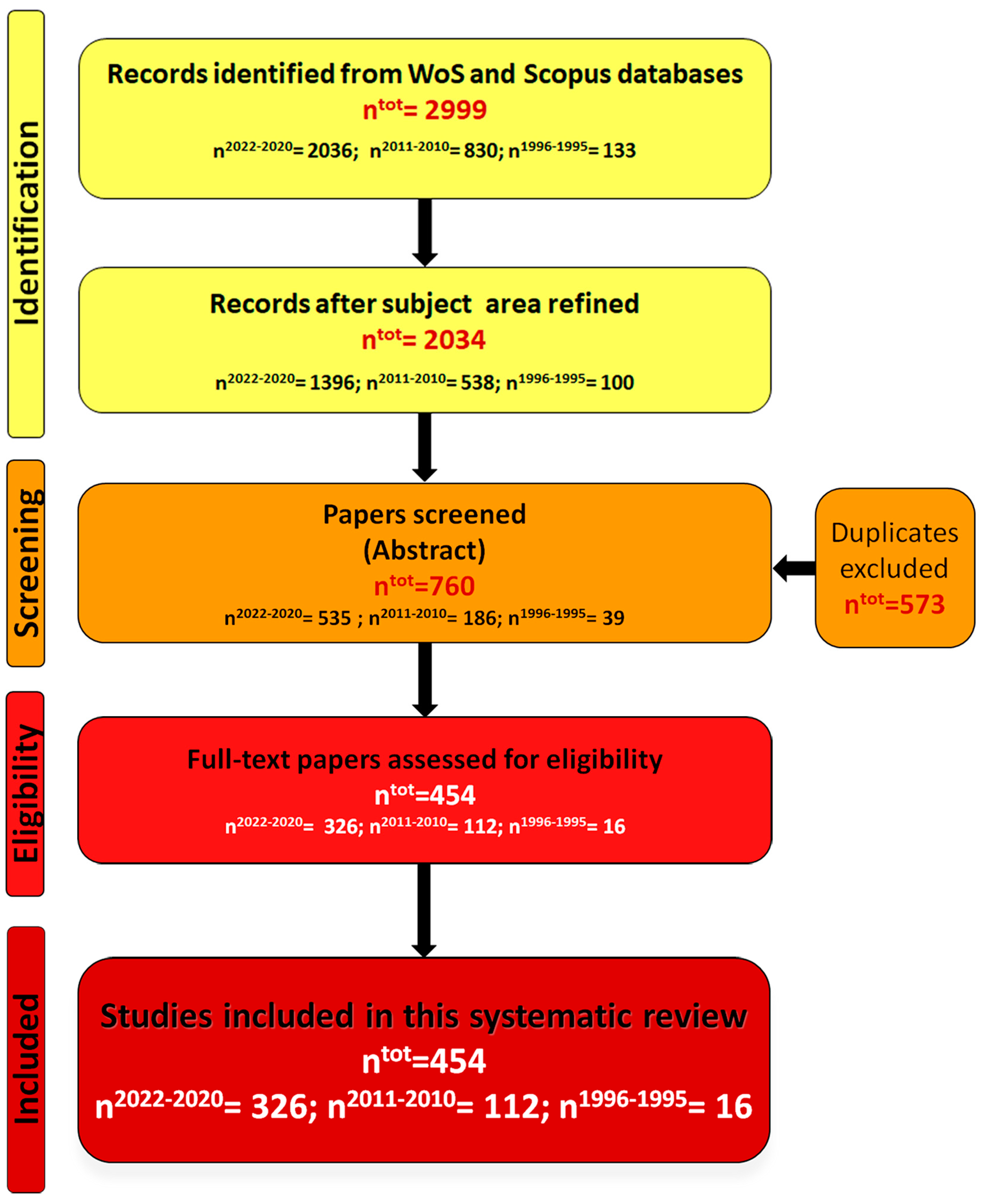
Initially, the papers that named the spectral unmixing in the titles, abstracts, and keywords were identified. For this purpose, all the names assigned to spectral unmixing (i.e., hyperspectral unmixing, linear mixing, nonlinear spectral mixing models, semi-empirical mixing model, spectral mixing models, spectral mixture analysis, spectral mixture modeling, spectral unmixing) were employed as unique query strings (first yellow box in Figure 1).
The total records identified from these databases was 2999. The subject areas of the search engines were checked to refine the identification of the papers. Therefore, “4.169 Remote Sensing”, “4.174 Digital Signal Processing”, “4.17 Computer Vision & Graphics”, “5.250 Imaging &Tomography”, “5.20 Astronomy & Astrophysics”, “5.191 Space Sciences”, “8.8 Geochemistry, Geophysics & Geology”, “8.93 Archaelogy”, “8.19 Oceanography, Meteorology & Atmospheric”, “8.140 Water Resources”, “8.124 Environmental Sciences”, “3.40 Forestry”, and “3.45 Soil Science” were “Citation Topics” selected in the WoS database, whereas “Earth and Planetary Sciences”, “Physics and Astronomy”, and “Environmental Science” were the subject areas selected in the Scopus database. After refining the subject areas, the identified papers became 2034 (second yellow box in Figure 1): 1396 were the papers published in 2022, 2021, and 2020; 538 were the papers published in 2011 and 2010; 100 were the papers published in 1996 and 1995.
2.2. Screening and Eligible Criteria
Reading the abstracts of the identified papers was conducted to select only those that applied spectral unmixing to remote images. Excluding the duplicates, 760 papers were selected with the first screening (orange box in Figure 1): 535 were the papers published in 2022, 2021, and 2020; 186 were the papers published in 2011 and 2010; 100 were the papers published in 1996 and 1995.
Reading the full text of the screened papers was conducted to identify only those that spatially validated the spectral unmixing results (bright red box in Figure 1). The last analysis identified the eligible papers: 326 were the papers published in 2022, 2021, and 2020; 112 were the papers published in 2011 and 2010; 16 were the papers published in 1996 and 1995.
In conclusion, 454 eligible papers were included in this systematic review. In Appendix A, the Table A1, Table A2, Table A3, Table A4, Table A5, Table A6 and Table A7 summarize the characteristics of the eligible papers that were published in 2022, 2021, 2020, 2011, 2010, 1996, and 1995, respectively.
3. Results
3.1. Spatial Validation of Spectral Unmixing Results
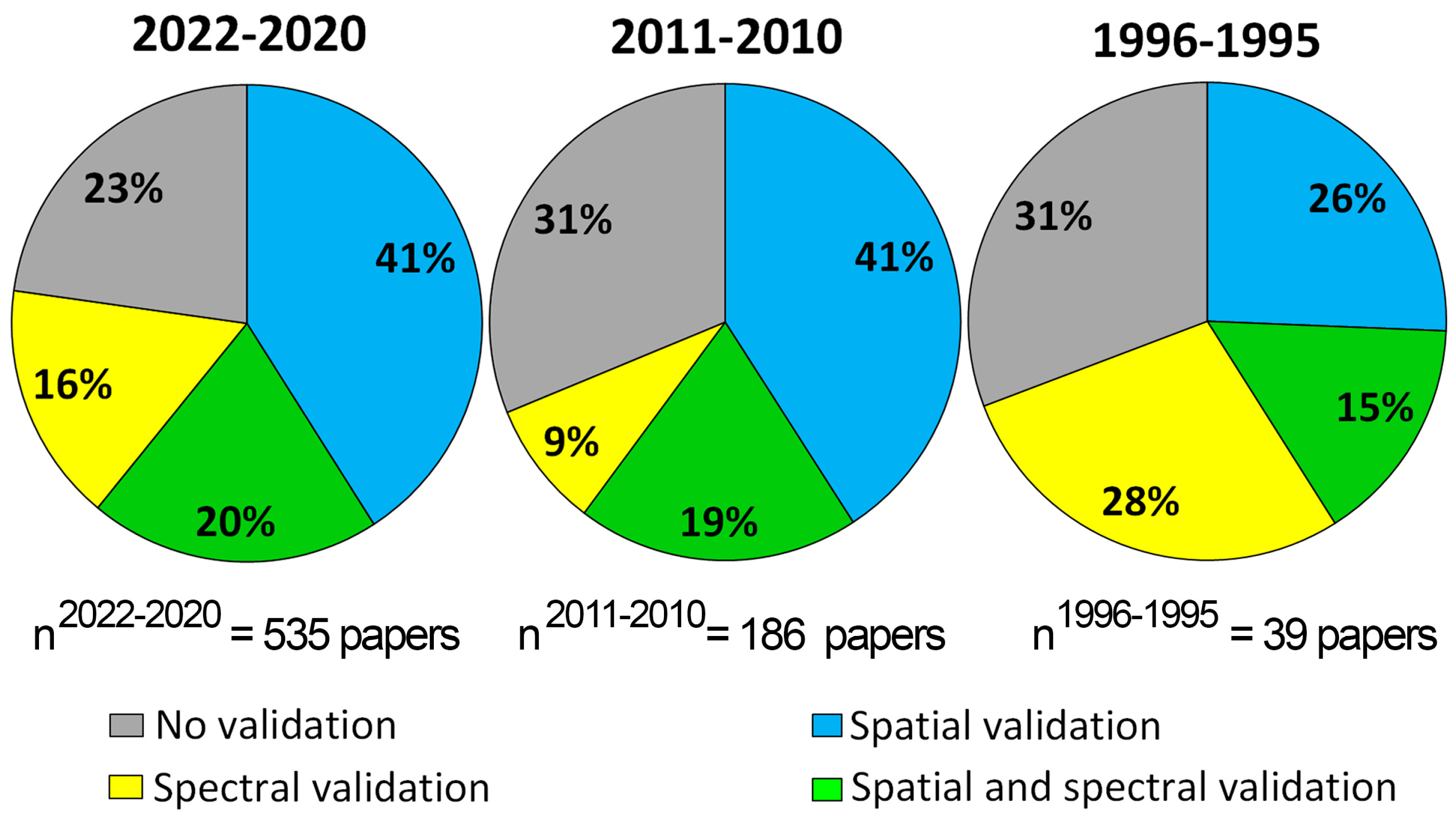
The screening carried out showed that the number of studies that spatially validated the results of spectral unmixing has significantly increased over the selected years (bright red box in Figure 1): about 100 research papers per year were published in the past 3 years; about 50 research papers per year were published in 2011 and 2010; about 10 research papers per year were published in 1996 and 1995. The screening carried out showed also that the number of studies that applied spectral unmixing has significantly increased over the selected years (orange box in Figure 1): about 180 research papers per year were published in the past 3 years; about 90 research papers per year were published in 2011 and 2010; about 20 research papers per year were published in 1996 and 1995. In order to assess the importance of spatial validation in the spectral unmixing procedure, the papers that applied spectral unmixing to remote imaging were analyzed (orange box in Figure 1). Figure 2 shows the percentage of these papers that were not validated (the percentage in grey wedges), spectrally validated (the percentage in yellow wedges), spatially validated (the percentage in blue wedges), and spatially and spectrally validated (the percentage in green wedges) the spectral unmixing results. Therefore, spatial validation was carried out alone (blue wedges in Figure 2) or together with spectral validation (green wedges in Figure 2).
Considering all papers that performed spatial validation (blue and green wedges in Figure 2), the percentage of these research published in 2022, 2021, and 2020 (61% of a total of 326 papers) was comparable to that of the papers that were published in 2011 and 2010 (60% of a total of 112 papers), whereas these percentages were greater than those of the papers that were published in 1996 and 1995 (41% of a total of 16 papers). Moreover, the percentage of the research published in 2022, 2021, and 2020 that did not validate the results (23%) was smaller than those of the papers that were published in the other 2 groups of years (31%). In conclusion, these values highlighted not only the increasing application of spectral unmixing over these years, but also the high priority given to the spatial validation.
3.2. Remote Images
The eligible papers published in 2022, 2021, 2020, 2011, 2010, 1996, and 1995 are summarized in Table 3, Table 4, Table 5, Table 6, Table 7, Table 8 and Table 9, according to the remote images to which spectral unmixing was applied. Authors who applied only spatial validation were cited in the fourth columns of Table 3, Table 4, Table 5, Table 6, Table 7, Table 8 and Table 9, whereas those who applied both spatial and spectral validation were cited in the fifth columns.

Table 3.
Eligible papers published in 2022.
| Remote Image Analyzed | Time Series | Study Area Scale | Spatial Validation Carried Out | Spatial and Spectral Validation Carried Out |
|---|---|---|---|---|
| AMMIS * (0.5 m) [55] | No | Local | [56,57] | |
| Apex * (2.5 m) [58] | No | Local | [59] | |
| ASTER (15–30–90 m) [60] | No | Regional 1 | [61] | |
| ASTER (15–30 m) | Yes 2 | Local | [62] | |
| AVHRR (1–5 km) [63] | Yes 1 | Regional 1 | [64] | [65,66] |
| AVIRIS * (10/20 m) [67] | No | Local | [57,68,69,70,71,72,73,74,75,76,77,78,79,80,81,82,83,84,85,86,87] | [88,89,90,91,92,93,94,95,96,97,98] |
| AVIRIS-NG * (5 m) [99] | No | Local | [100] | |
| CASI * (2.5 m) [101] | No | Local | [59,78] | |
| DESIS * (30 m) [102] | Yes 1 | Regional 1 | [103] | |
| DESIS * (30 m) | No | Local | [104] | |
| EnMap * (30 m) [105] | No | Local | [69] | |
| GaoFen-6 (2–8–16 m) [106] | No | Regional 1 | [107] | |
| GaoFen-2 (3.2 m) | Yes 1 | Regional 1 | [108] | |
| GaoFen-1 (2–8–16 m) | No | Local | [109] | |
| HYDICE * (10 m) [110] | No | Local | [59,68,76,77,79,81,82,85,86,90,111] | [89,96,97] |
| Hyperion * (30 m) [112] | Yes 1 | Local | [75] | |
| Hyperion * (30 m) | No | Local | [113] | [114,115,116] |
| HySpex * (0.6–1.2 m) [104] | No | Local | [104,117] | |
| Landsat (15–30 m) [118] | Yes 1 | Continental 1 | [119] | |
| Landsat (15–30 m) | Yes 1 | Regional 1 | [108,120,121,122,123,124,125,126,127,128,129,130,131,132,133] | [134,135] |
| Landsat (15–30 m) | No | Regional 1 | [107,136,137] | |
| Landsat (15–30 m) | Yes 1 | Local | [138,139] | [62] |
| Landsat (15–30 m) | No | Local 2 | [140,141] | |
| Landsat (15–30 m) | No | Local | [109,142] | |
| M3 hyperspectral image * [143] | No | Moon | [143] | |
| MIVIS * (8 m) [144] | No | Local | [145] | |
| MERIS (300 m) [146] | Yes 1 | Local | [147] | |
| MODIS (0.5–1 km) [148] | Yes 1 | Continental 1 | [149] | |
| MODIS (0.5 km) | Yes 1 | Regional 1 | [108,150,151,152] | [137] |
| MODIS (0.5 km) | No | Local | [153] | |
| NEON * (1 m) [154] | No | Local | [154] | |
| PRISMA * (30 m) [155] | No | Local | [114,156,157,158] | |
| ROSIS * (4 m) [159] | No | Local | [56,57,78,81,85] | |
| Samson * (3.2 m) [59] | No | Local | [59,72] | [89,97] |
| Sentinel-2 (10–20–60 m) [160] | Yes 1 | Regional 1 | [108,133,161,162,163] | |
| Sentinel-2 (10–20–60 m) | No | Regional 1 | [136] | [107,164,165] |
| Sentinel-2 (10–20–60 m) | Yes 1 | Local | [166,167] | [168] |
| Sentinel-2 (10–20–60 m) | No | Local 2 | [104] | |
| Sentinel-2 (10–20–60 m) | No | Local | [169] | |
| Specim IQ * [170] | Yes 1 | Laboratory | [170] | |
| SPOT (10–20 m) [171] | No | Local 2 | [140] | |
| WorldView-2 (0.46–1.8 m) [172] | No | Local | [166] | |
| WorldView-3 (0.31–1.24–3.7 m) | No | Local | [166] |
* Hyperspectral sensor; 1 Multiple images acquired from same sensor; 2 Multiple images acquired from different sensors.
Table 4.
Eligible papers published in 2021.
| Remote Image Analyzed | Time Series | Study Area Scale | Spatial Validation Carried Out | Spatial and Spectral Validation Carried Out |
|---|---|---|---|---|
| ASTER (15–30–90 m) | No | Regional 1 | [173] | |
| AVIRIS * | No | Local | [174,175,176,177,178,179,180,181,182,183,184,185,186,187,188,189,190,191,192,193,194,195,196,197,198,199,200,201] | [202,203,204,205,206,207,208,209,210,211,212,213,214,215,216,217,218,219,220,221,222,223,224,225] |
| AVIRIS-NG * (5 m) | No | Local | [226] | |
| CASI * | No | Local | [174,227] | |
| Simulated EnMAP * | Yes 1 | Regional 1 | [228] | |
| GaoFen-5 * (30 m) | No | Local | [229] | |
| HYDICE * (10 m) | No | Local | [192,230,231,232] | [204,212,214,216,218] |
| HyMap * (4.5 m) | Yes | Local | [233] | |
| Hyperion * (30 m) | No | Local | [212,234,235] | |
| Hyperion * (30 m) | Yes 1 | Local | [236,237] | |
| HySpex | No | Local | [238] | |
| Landsat (30 m) | Yes 1 | Regional 1 | [239,240,241,242,243,244] | |
| Landsat (30 m) | Yes 1 | Local 2 | [245,246,247,248,249,250,251,252,253] | |
| Landsat (30 m) | No | Local | [227,254,255,256,257,258,259] | |
| Landsat (30 m) | No | Regional 1 | [260] | |
| MODIS (0.5–1 km) | No | Local | [254,261] | |
| MODIS (0.5–1 km) | Yes 1 | Regional 1 | [262,263,264] | |
| PRISMA * (30 m) | No | Local | [265] | |
| ROSIS * (4 m) | No | Local | [191,200,266] | [217,267] |
| Samson * (3.2 m) | No | Local | [188,232,268] | [207,210,211,214,224,225,267] |
| Sentinel-2 (10–20–60 m) | No | Local | [255,258] | [226,269] |
| Sentinel-2 (10–20–60 m) | Yes 1 | Local | [243,253,270] | [229,271,272] |
| Sentinel-2 (10–20–60 m) | No | Regional 1 | [273] | |
| Sentinel-2 (10–20–60 m) | Yes 1 | Regional 1 | [244] | |
| UAV multispectral image [274] | No | Local | [274] | |
| WorldView-2 (0.46–1.8 m) | Yes 1 | Local | [275] | |
| WorldView-3 (0.31–1.24–3.7 m) | No | Local 2 | [276] | |
| ZY-1-02D * (30 m) [228] | No | Local | [228] |
* Hyperspectral sensor; 1 Multiple images acquired from same sensor; 2 Multiple images acquired from different sensors.
Table 5.
Eligible papers published in 2020.
| Remote Image Analyzed | Time Series | Study Area Scale | Spatial Validation Carried Out | Spatial and Spectral Validation Carried Out |
|---|---|---|---|---|
| AISA Eagle II airborne hyperspectral scanner * [277] | No | Local | [277] | |
| ASTER (15–30–90 m) | No | Regional 1 | [278] | |
| ASTER (15–30–90 m) | Yes 1 | Local 2 | [279,280] | |
| AVIRIS * | No | Local | [281,282,283,284,285,286,287,288,289,290,291,292,293,294,295,296,297,298] | [299,300,301,302,303,304,305,306,307,308,309,310,311,312,313,314,315,316,317,318,319,320,321,322,323,324,325,326,327] |
| AVIRIS NG * | No | Local | [291] | |
| AWiFS [328] | Yes 1 | Local 2 | [328] | |
| CASI * | No | Local | [329] | |
| Simulated EnMAP * (30 m) | No | Regional 1 | [330] | |
| GaoFen-1 WFV | Yes 1 | Local | [331] | |
| GaoFen-1 WFV | Yes 1 | Local 2 | [332] | [333] |
| GaoFen-2 | No | Local 2 | [332] | |
| HYDICE * (10 m) | No | Local | [292,293,298,334,335] | [299,307,309,310,316,318,321,322,324] |
| HyMAP * | No | Local 2 | [280] | |
| HyMAP * | No | Local | [336] | |
| HySpex * (0.7 m) | No | Local | [337] | |
| Hyperion * (30 m) | No | Local | [336] | [338] |
| Landsat (30 m) | Yes 1 | Local 2 | [332] | [280,339] |
| Landsat (30 m) | Yes 1 | Local | [252,340,341,342,343,344,345,346,347] | |
| Landsat (30 m) | Yes 1 | Continental 1 | [348] | |
| Landsat (30 m) | Yes 1 | Regional 1 | [349,350,351,352,353,354,355] | [356] |
| Landsat (30 m) | No | Regional 1 | [357] | |
| MODIS (0.5–1 km) | Yes 1 | Local | [340,358,359,360,361] | [333] |
| MODIS (0.5–1 km) | Yes 1 | Regional 1 | [362,363] | |
| MODIS (0.5–1 km) | Yes 1 | Local 2 | [364,365] | [279] |
| PlanetScope (3 m) [366] | Yes 1 | Local 2 | [366] | |
| PROBA-V (100 m) [367] | Yes 1 | Regional 1 | [353,368,369,370,371] | |
| ROSIS * (4 m) | No | Local | [285,372] | [373] |
| Samson * (3.2 m) | No | Local | [284,374,375] | [301,303,305,315,320,323,324] |
| Sentinel-2 (10–20–60 m) | No | Local 2 | [332,376] | [280,339] |
| Sentinel-2 (10–20–60 m) | Yes 1 | Local | [328,340,377,378,379,380,381,382] | [333,383] |
| Suomi NPP-VIIRS [354] | Yes 1 | Regional 1 | [353] | |
| UAV hyperspectral data * [384] | Yes 1 | Local | [384] | |
| WorldView-2 | Yes 1 | Local | [342] | |
| WorldView-2 | Yes 1 | Local 2 | [385] | |
| WorldView-3 | Yes 1 | Local 2 | [385] |
* Hyperspectral sensor; 1 Multiple images acquired from same sensor; 2 Multiple images acquired from different sensors.
Table 6.
Eligible papers published in 2011.
| Remote Image Analyzed | Time Series | Study Area Scale | Spatial Validation Carried Out | Spatial and Spectral Validation Carried Out |
|---|---|---|---|---|
| AHS * [386] | No | Local | [386] | |
| ASTER | No | Local | [387,388,389] | |
| ASTER | Yes 1 | Local | [390,391] | |
| AVIRIS * | No | Local | [307,392,393,394,395,396,397,398,399,400,401,402,403] | [387,404,405,406,407,408,409,410,411,412,413,414,415,416,417] |
| CASI * | No | Local | [418] | |
| MERIS (300 m) | No | Local | [419] | |
| MODIS (0.5–1 km) | Yes 1 | Local | [420,421,422,423] | |
| HYDICE * | No | Local | [392,424] | [414,415,425] |
| HyMAP * | No | Local | [392,426] | [427] |
| Hyperion * (30 m) | No | Local | [387,428] | |
| HJ-1 * (30 m) [429] | No | Local | [429,430] | |
| Landsat (30 m) | Yes 1 | Local | [431,432,433] | [387] |
| Landsat (30 m) | No | Local | [434,435] | |
| Landsat (30 m) | Yes 1 | Local 2 | [436,437,438] | |
| Landsat (30 m) | No | Local 2 | [423,439] | |
| QuickBird (0.6–2.4 m) [440] | No | Local | [441,442] | |
| SPOT (10–20 m) | No | Local 2 | [439,441] |
* Hyperspectral sensor; 1 Multiple images acquired from same sensor; 2 Multiple images acquired from different sensors.
Table 7.
Eligible papers published in 2010.
| Remote Image Analyzed | Time Series | Study Area Scale | Spatial Validation Carried Out | Spatial and Spectral Validation Carried Out |
|---|---|---|---|---|
| Airborne hyper-spectral image * (about 1.5 m) [443] | No | Regional 1 | [443] | |
| AHS * (2.4 m) | No | Local | [444] | |
| ASTER (15–30–90 m) | Yes 1 | Local | [445,446] | |
| ASTER (15–30–90 m) | Yes 1 | Regional 1 | [447] | |
| ATM (2 m) [101] | No | Local 2 | [101] | |
| AVHRR (1 km) | Yes 1 | Regional 1 | [448] | |
| AVIRIS * (20 m) | No | Local | [449,450,451,452,453,454,455,456,457] | [458,459,460,461,462,463] |
| CASI * (2 m) | No | Local | [101] | |
| CASI * | No | Laboratory | [464,465] | |
| CHRIS * (17 m) [466] | No | Local | [467] | |
| DAIS * (6 m) [464] | No | Local | [465] | |
| DESIS * | No | Local | [468,469] | |
| HYDICE * | No | Local | [455,470,471] | [458,463] |
| HyMAP * | No | Local | [471] | |
| Hyperion * (30 m) | No | Local | [472,473,474] | |
| HJ-1 * (30 m) | No | Local | [475,476] | |
| Landsat (30 m) | Yes 1 | Regional 1 | [477,478,479,480,481,482,483] | |
| Landsat (30 m) | No | Regional 1 | [484,485,486,487,488,489] | [490] |
| Landsat (30 m) | No | Local 2 | [491,492] | |
| Landsat (30 m) | No | Local | [493] | |
| MIVIS * (3 m) | No | Regional 1 | [494] | |
| MODIS (0.5–1 km) | Yes 1 | Regional 1 | [495] | |
| MODIS (0.5–1 km) | Yes 1 | Continental 1 | [496] | |
| QuickBird (2.4 m) | No | Local 2 | [491] | |
| QuickBird (2.4 m) | No | Local | [497,498] | |
| SPOT (10–20 m) | Yes 1 | Regional 1 | [480] | |
| SPOT (2.5–10–20 m) | No | Local 2 | [486,491,492] | |
| SPOT (2.5–10–20 m) | No | Local | [499] | [500] |
* Hyperspectral sensor; 1 Multiple images acquired from same sensor; 2 Multiple images acquired from different sensors.
Table 8.
Eligible papers published in 1996.
| Remote Image Analyzed | Time Series | Study Area Scale | Spatial Validation Carried Out | Spatial and Spectral Validation Carried Out |
|---|---|---|---|---|
| AVIRIS * | No | Local | [501,502] | [503] |
| GERIS * [504] | No | Local | [504] | |
| Landsat (30 m) | No | Local | [14,505] | [506] |
| SPOT (2.5–10–20 m) | No | Local | [507] |
* Hyperspectral sensor.
Table 9.
Eligible papers published in 1995.
| Remote Image Analyzed | Time Series | Study Area Scale | Spatial Validation Carried Out | Spatial and Spectral Validation Carried Out |
|---|---|---|---|---|
| AVHRR (1–5 km) | Yes 1 | Regional 1 | [508] | |
| AVIRIS * (20 m) | No | Local | [509] | [510,511] |
| Landsat (30 m) | No | Local | [512] | [513] |
| MIVIS * (4 m) | No | Local | [514] | |
| MMR * [515] | Yes 1 | Local | [515] |
* Hyperspectral sensor; 1 Multiple images acquired from same sensor.
The first columns of Table 3, Table 4, Table 5, Table 6, Table 7, Table 8 and Table 9 and the second columns of Table A1, Table A2, Table A3, Table A4, Table A5, Table A6 and Table A7 show the sensor name and the spatial resolution of the images. Considering all eligible papers, 27 hyperspectral sensors and 16 multispectral sensors were employed. Hyperspectral sensors were highlighted in the first columns of Table 3, Table 4, Table 5, Table 6, Table 7, Table 8 and Table 9 with an asterisk. The literature often combined spectral unmixing with hyperspectral data because the number of bands must be greater than the number of endmembers [4,5,42,44]. However, the percentage of papers that employed hyperspectral data (57% of a total of 458 papers) is slightly higher than the percentage of papers that employed multispectral data (43% of a total of 458 papers). The second columns of Table 3, Table 4, Table 5, Table 6, Table 7, Table 8 and Table 9 show the papers that performed the time series studies, whereas the third columns of these tables show the papers that performed the local, regional, or continental studies.
The analysis of these data showed that most studies that analyzed hyperspectral images were performed at the local scale and did not carry out the multitemporal studies, whereas most studies that analyzed multispectral images were performed at the regional or continental scale and carried out the multitemporal studies (more than one image was analyzed). Therefore, the spectral unmixing is widely applied to multispectral images, despite their smaller number of bands than hyperspectral images, because these data are characterized by greater spatial and temporal availability than those of the hyperspectral data.
Moreover, the spectral unmixing was also applied to some hyperspectral and multispectral images that were characterized with high spatial resolutions (e.g., AMMIS image with spatial resolution equal to 0.5 m [56] and WorldView-3 image with spatial resolution of 0.31 m [166]). These papers confirm that, no matter how high the spatial resolution might be, no image pixel results were completely homogeneous in spectral characteristics [9,516,517].
3.3. Accuracy Metrics
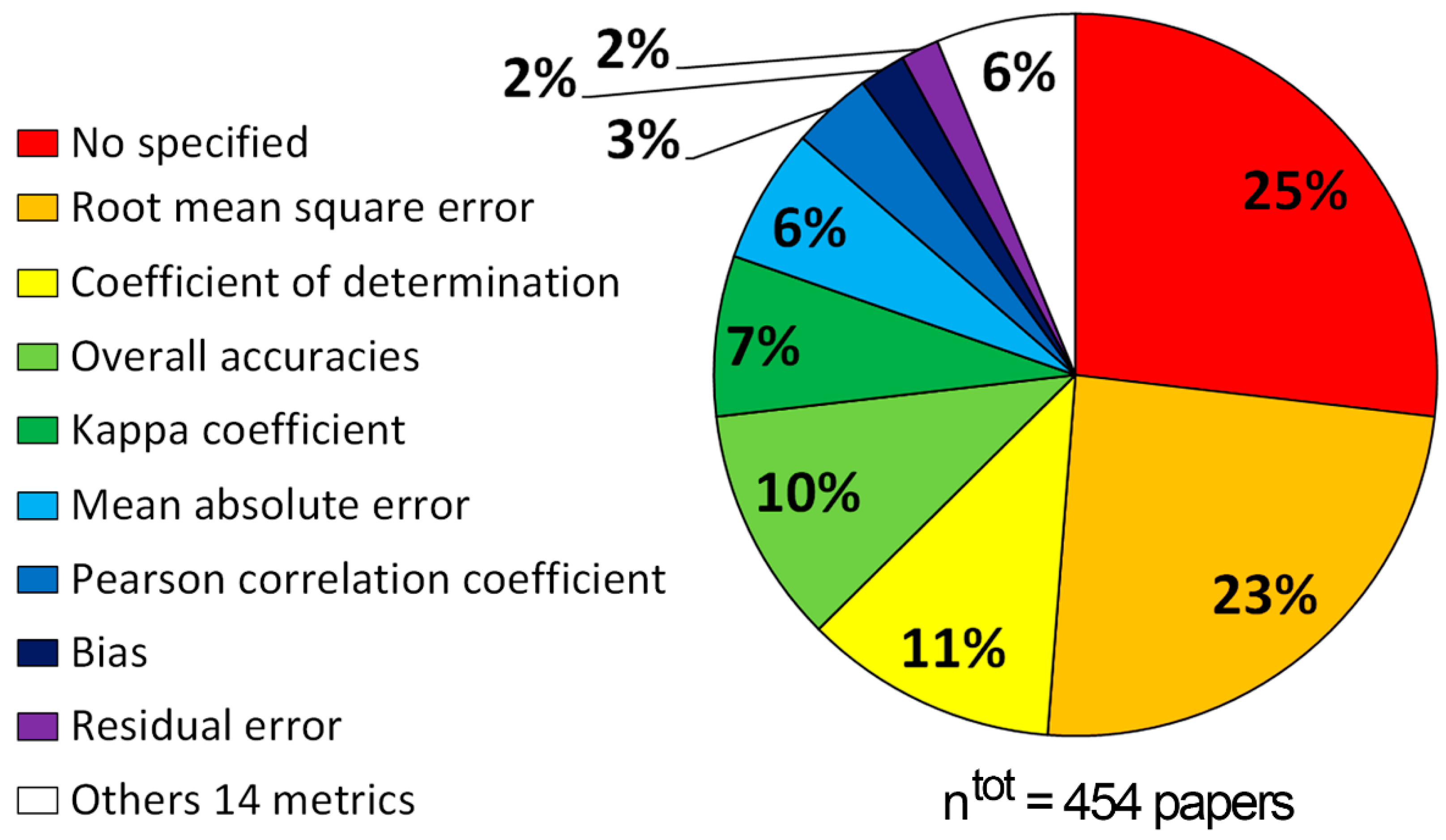
Accuracy, which is defined as “the degree of correctness of the map”, is usually assessed by comparing the “ground truth” with the map retrieved from remote images [518,519]. Because no map can fully and completely map the territory [520], ground truth is more correctly called reference data [521]. To assess the differences between the reference data and results of the spectral unmixing, the eligible papers exploited different metrics. Figure 3 shows the pie chart of the distribution of the metrics that were adopted by eligible papers.
The other 14 metrics were average accuracy [522], correct labeling percentage for the unchanged pixels [141], correlation coefficient [150], Kling–Gupta efficiency [523], mean abundance error [117], mean error [169], mean relative error [169], normalized average of spectral similarity measures [524], producer’s accuracy [153], Receiver Operating characteristic Curves (ROC) method [525], relative mean bias [165], separability spectral index [526], signal-to-reconstruction error [56], and systematic error [109].
In conclusion, the authors of 454 eligible papers employed 22 different metrics, and most authors employed more than 1 metric. Overall, 25% of the eligible papers did not specify the accuracy metrics used. It is very important to note that some standard accuracy assessments, such as the kappa coefficient, “assume implicitly that each of the testing samples is pure”; therefore, some of these metrics were inappropriate for evaluating the accuracy of the fractional abundance maps [41,518].
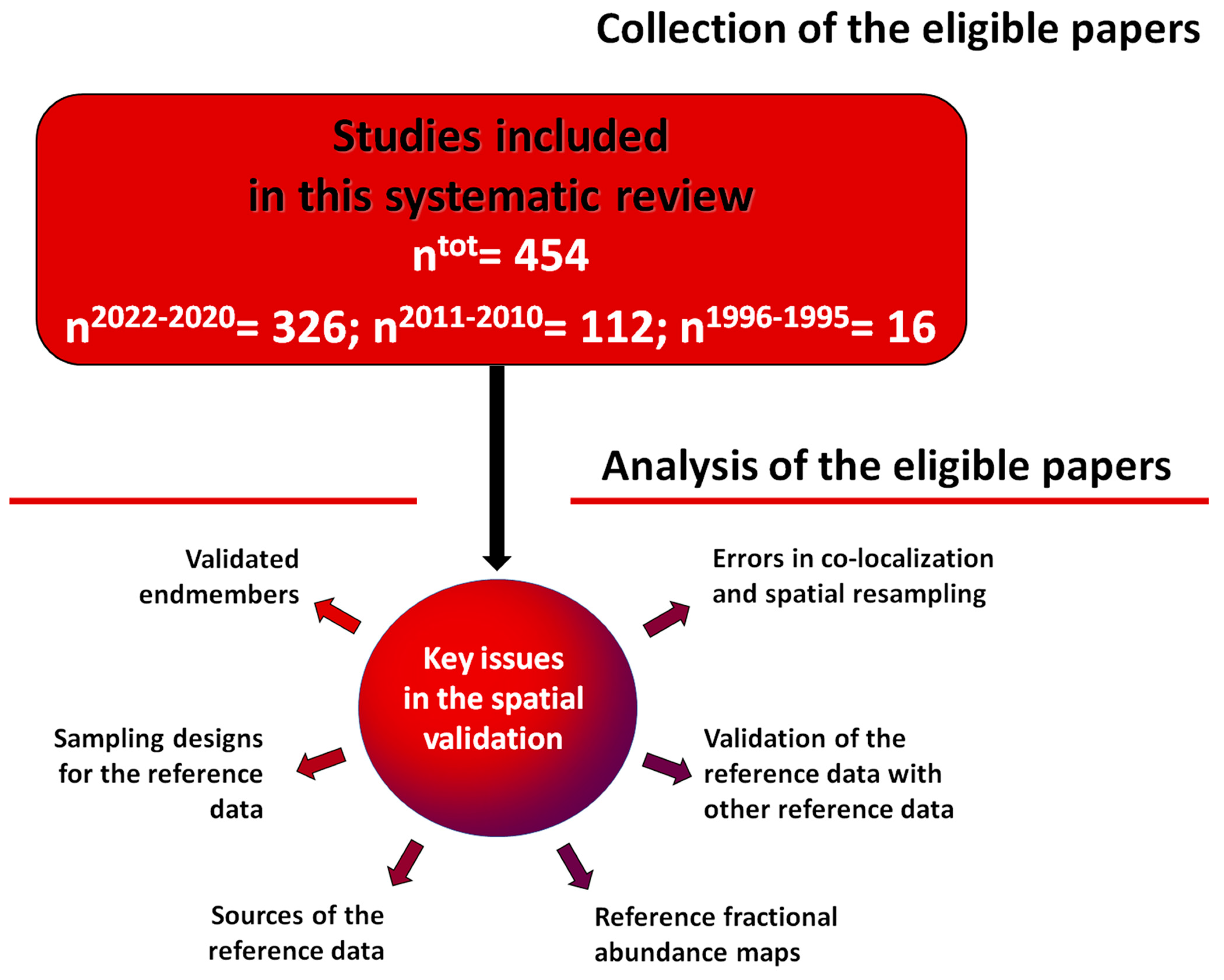
3.4. Key Issues in the Spatial Validation
Since the literature highlighted many sources of error in accuracy assessment of retrieved maps [518,519,521], the authors identified and carried out several “key issues” to address and minimize these errors. Figure 4 and Table A1, Table A2, Table A3, Table A4, Table A5, Table A6 and Table A7 summarize the key issues that were identified.
3.4.1. Validated Endmembers
Before analyzing the endmembers that were validated, it is necessary to remember that the number of endmembers that were determined with the images must be less than the number of sensor bands; therefore, the number of endmembers that were determined with the multispectral data is less than the number of endmembers that were determined with the hyperspectral data [6,23,527]. Therefore, the authors who elaborated the multispectral images employed smaller levels of model complexity than authors who elaborated the hyperspectral images [528,529]. For example, the VIS model was used to map only three endmembers (Vegetation, Impervious surfaces, and Soil) in many urban areas that were retrieved from multispectral data (e.g., [109,152,477,493]).
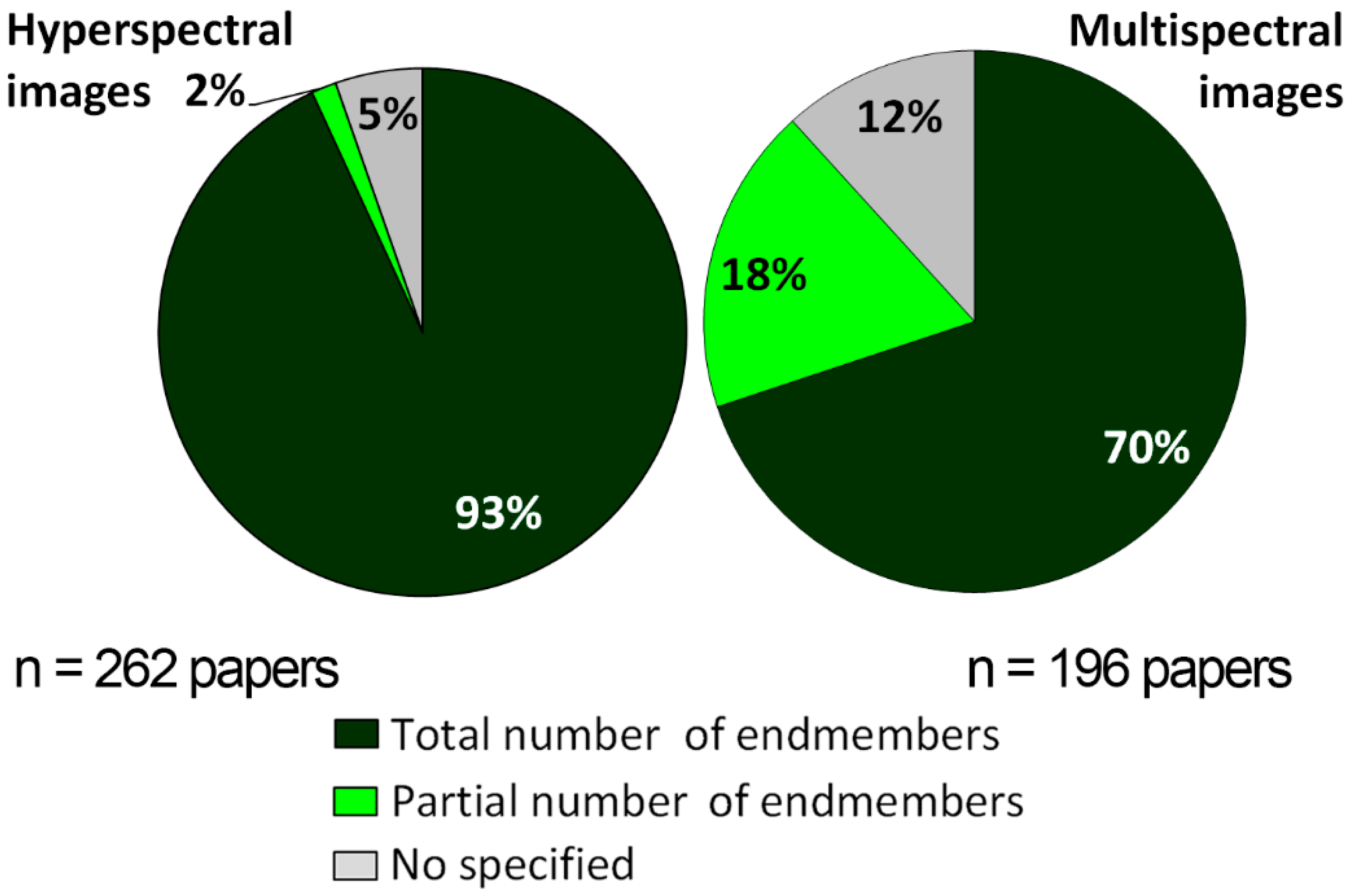
The third columns of Table A1, Table A2, Table A3, Table A4, Table A5, Table A6 and Table A7 list the endmembers that were determined using spectral unmixing; the fourth columns of these showed the number of these endmembers that were validated. It is interesting to note that some authors validated smaller number of endmembers than the number of the endmembers that were determined (i.e., 40 eligible papers). Dividing the works that analyzed hyperspectral images from those that analyzed multispectral data, Figure 5 shows the percentage of studies that validated the total or partial number of endmembers. It is important to highlight that, since 4 eligible papers analyzed both hyperspectral and multispectral data [104,227,231,281], the sum of papers that analyzed hyperspectral data and papers that analyzed multispectral data (i.e., 458) is greater than the number of eligible papers (i.e., 454).
Therefore, only 2% of the studies that elaborated hyperspectral images partially validated the determined endmembers, whereas 18% of the studies that elaborated multispectral images partially validated the determined endmembers. As mentioned above, hyperspectral images were used to carry out non-repeated surveys over time and at local-scale studies (252 papers of a total of 262), whereas most multispectral images were used to carry out regional- or continental-scale studies that were or were not repeated over time (180 papers of a total of 196). Therefore, some of these authors, who analyzed more than one image, chose to spatially validate only the materials or groups of materials on which they focused their study. For example, Hu et al. [149] spatially validated only blue ice fractional abundance maps that were retrieved from MODIS images covering the period 2000–2021 in order to present a FABIAN (Fractional Austral-summer Blue Ice over Antarctica) product. It should be noted that 5 and 12% of the papers that analyzed hyperspectral or multispectral data, respectively, did not specify which endmembers were validated.
3.4.2. Sampling Designs for the Reference Data
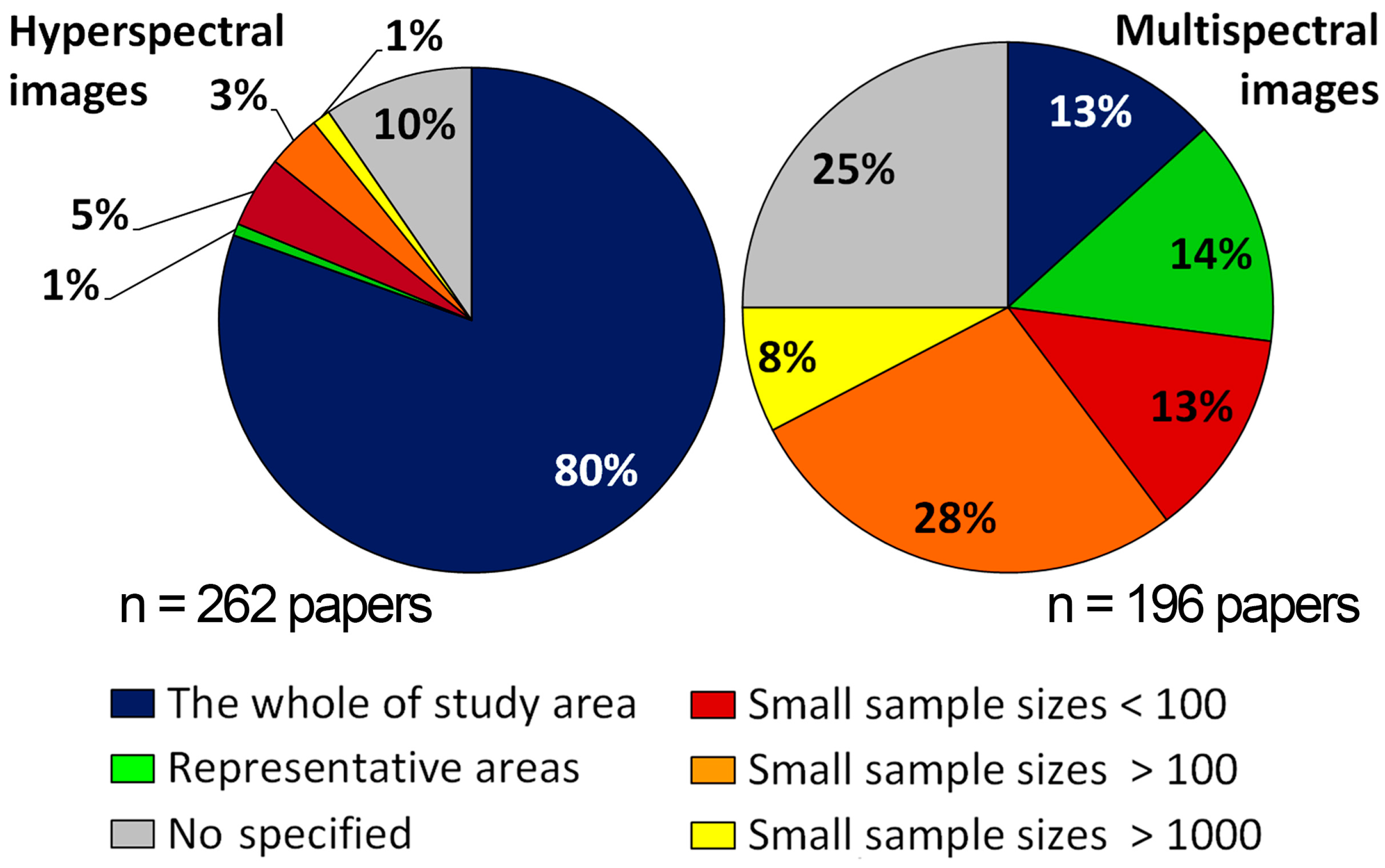
The literature demonstrated that a possible source of error in spatial validation is due to the choice of the sampling design for the reference data [518,519,521,530]. The sampling design mainly includes the definition of the sample size and the sampling design of the reference data [518]. Authors of eligible papers chose three kinds of sample sizes: the whole study area; the representative area; small sample sizes (pixels, plots, and polygons samples). The eighth columns of Table A1, Table A2, Table A3, Table A4, Table A5, Table A6 and Table A7 show the different sample sizes that were adopted by every eligible paper, and Table 10 shows the number of papers that adopted the different sample sizes.
Most authors of the eligible papers chose to validate the whole study areas, followed, in descending order, by the choice to employ the different number of small sample sizes and then the representative areas. It is also important to note the high percentages of the papers that did not specify the sample size of the reference data: 18, 11, and 31%, respectively.
The literature also pointed out that the sampling designs for spatially validating maps at local scale cannot be the same as the designs for spatially validating maps at regional or continental scale [518,530]. As mentioned above, most of the studies that analyzed the hyperspectral data were performed at local scale (252 papers of a total of 262), whereas the studies that analyzed the multispectral images performed at regional or continental scale (180 papers of a total of 196). Therefore, the eligible papers that analyzed hyperspectral images were analyzed separately from those that analyzed multispectral images (Figure 6 on the right and left, respectively), not only to analyze the different sampling designs adopted from the hyperspectral and multispectral data, but also to highlight the different sampling designs chosen for local or regional/continental scale studies. Figure 6 shows the percentage of the eligible papers that employed the different sample sizes and the percentage of the eligible papers that employed a different number of small sample sizes.
Most papers that processed hyperspectral images validated the whole study area (212 papers), whereas most papers that processed multispectral images employed small sample sizes (94 papers).
The authors of eligible papers that employed small sample sizes adopted three different sampling designs of reference data: partial, random, and uniform. The ninth columns of Table A1, Table A2, Table A3, Table A4, Table A5, Table A6 and Table A7 show the sampling designs of every eligible paper. Most authors who published in 2022, 2021, and 2020 and published in 2011 and 2010 chose the random distribution of reference data (78% for a total of 326 papers and 76% for a total of 110 papers, respectively), whereas the authors who published in 1996 and 1995 did not specify the sampling designs employed. Stehman and Foody [519] highlighted that “the most commonly used designs” that were chosen to assess the land cover products were “simple random, stratified random, systematic, and cluster” designs. Therefore, these results confirmed that random designs were the most commonly used approaches.
3.4.3. Sources of the Reference Data
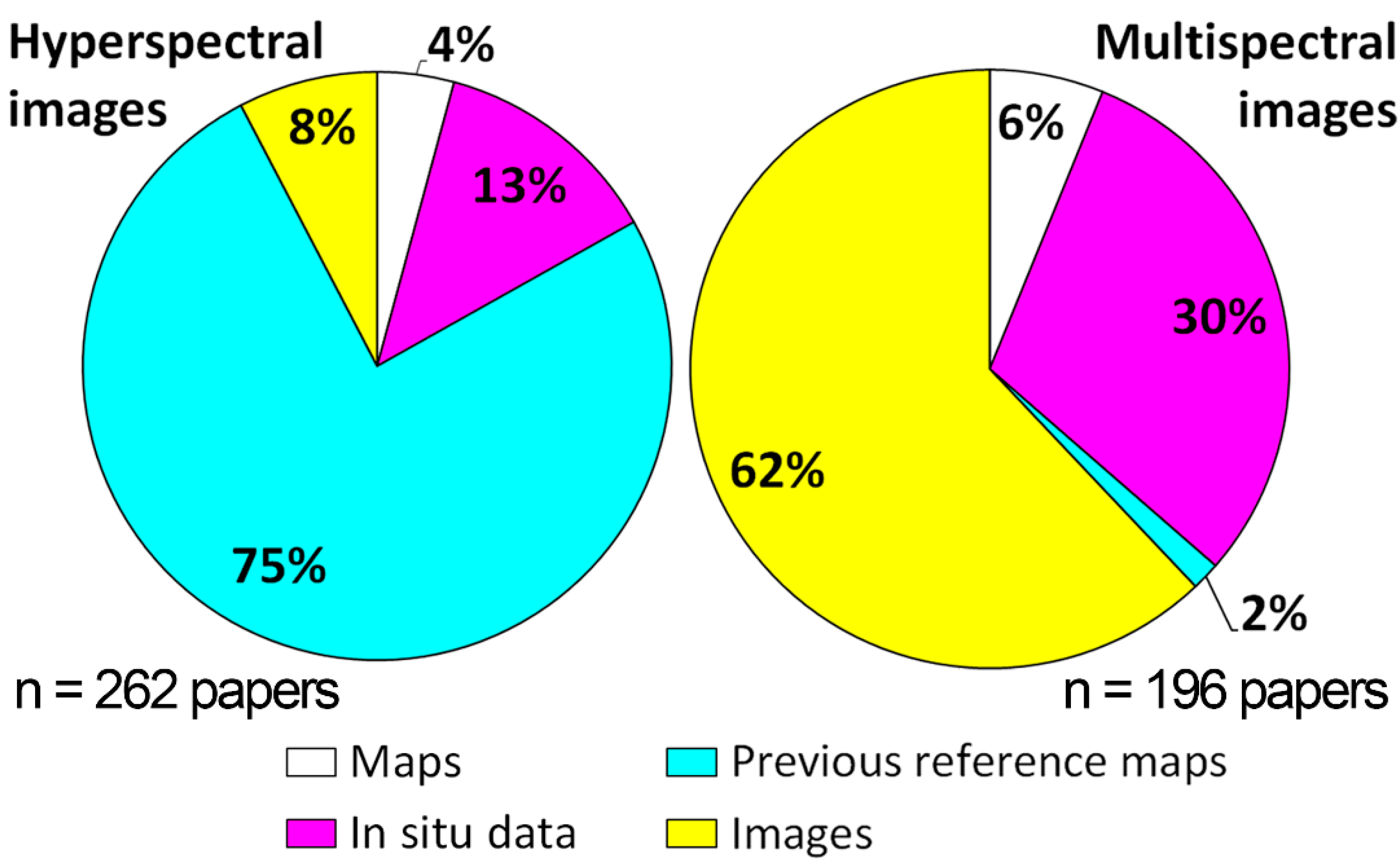
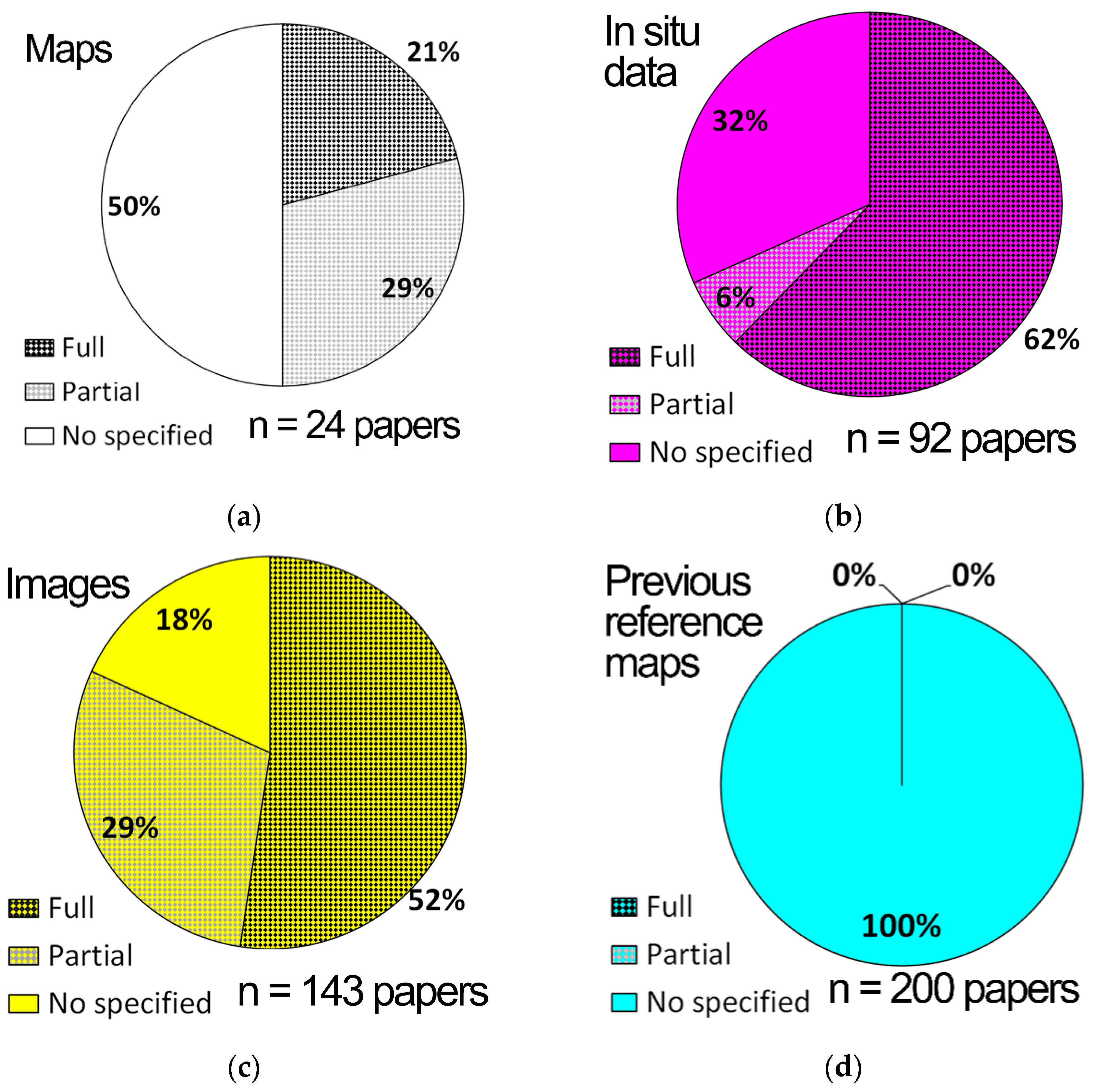
Eligible papers employed four different sources of reference data to spatially validate spectral unmixing results: images, in situ data, maps, and previous reference maps. Table 11 shows the number of the eligible papers that employed these reference data sources, whereas the fifth columns of Table A1, Table A2, Table A3, Table A4, Table A5, Table A6 and Table A7 detail the sources of the reference data.
The number of authors who chose to utilize geological, land use, or land cover maps as reference maps is the smallest (5% of the total eligible papers), followed, in ascending order, by the number who chose to create the reference maps using in situ data (20% of the total eligible papers), and then by the number of authors who chose to create the reference maps using other images (31% of the total eligible papers). Firstly, the number of authors who chose to use the previous reference maps is the largest (44% of the total eligible papers).
As regards the authors who chose to create the reference maps using other images, most of them employed images at higher spatial resolutions than those of the remote images analyzed (95% of a total of 143 papers). To create the reference maps from the images, 47% of the eligible papers did not specify the method used to map the endmembers, 29% employed the photo-interpretation, 21% classified the images, 2% used the vegetation indexes, and 2% used the mixed approach by classifying and/or photo-interpreting and/or applying vegetation indexes (e.g., [114,145,531]). As regards the classification methods, there are four works that applied the same classification procedure to analyze the remote images and to create the reference maps [65,66,149,261]. Among these, the authors of 3 papers compared the fractional abundance maps that were retrieved from the multispectral images at moderate spatial resolutions (10, 30, and 60 m) with the fractional abundance maps that were retrieved from the multispectral data at coarse spatial resolutions (0.5 and 1 km) [65,66,149].
Moreover, the reference data sources that were chosen to validate the results of the hyperspectral images were analyzed separately from those that were chosen to validate the results of the multispectral images. Figure 7 shows the percentage of the papers that adopted the different sources of the reference data to validate the results of hyperspectral (right) and multispectral data (left).
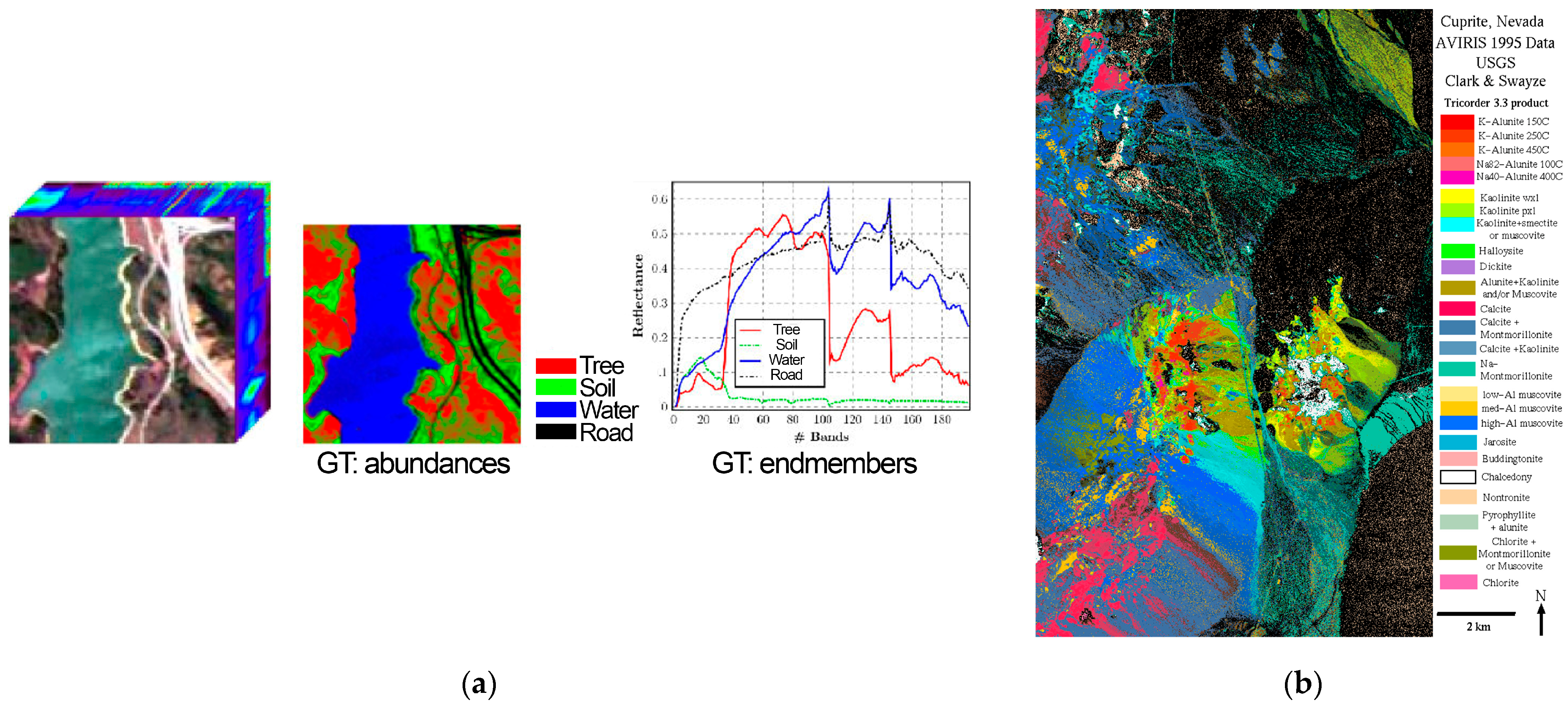
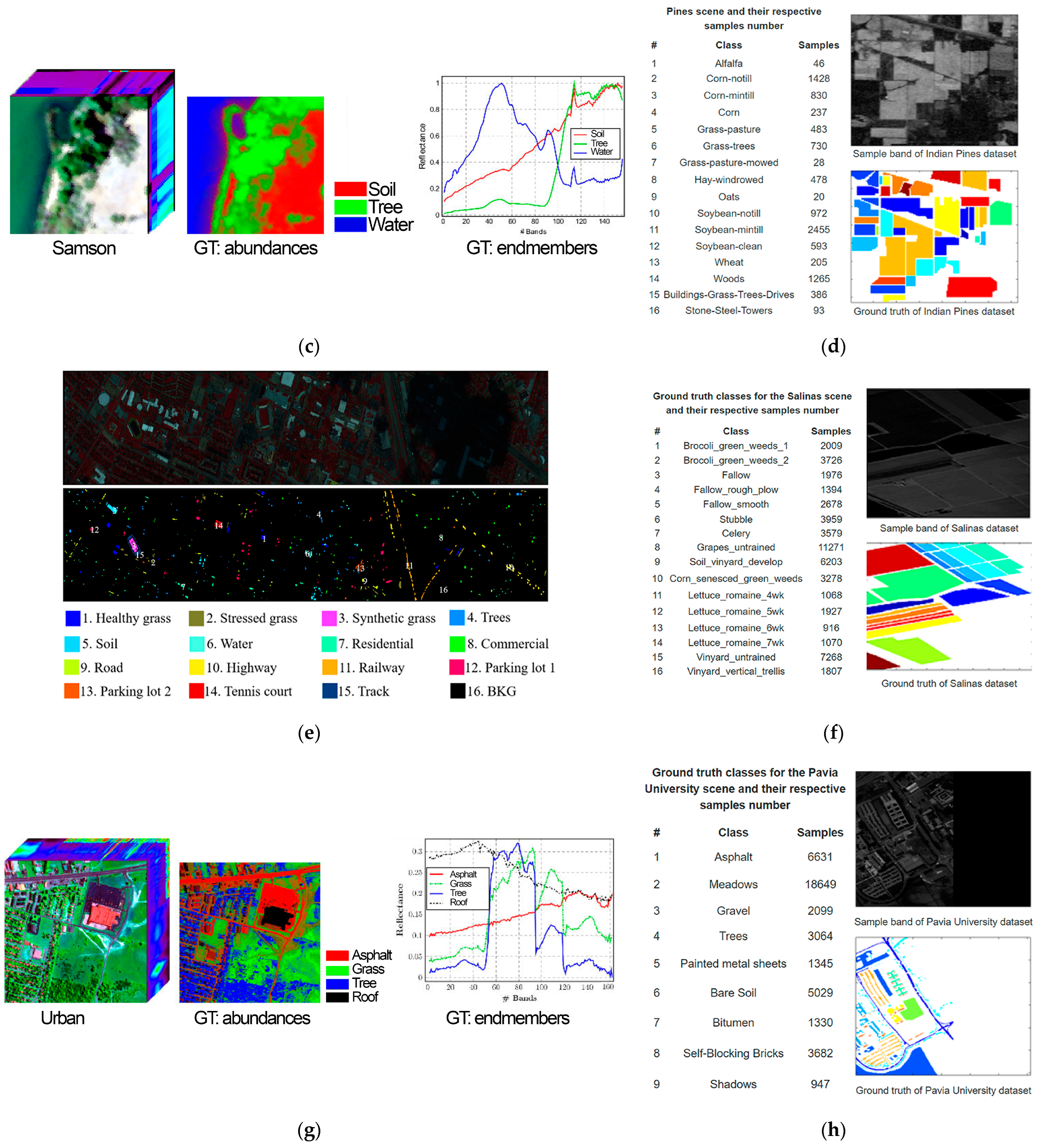
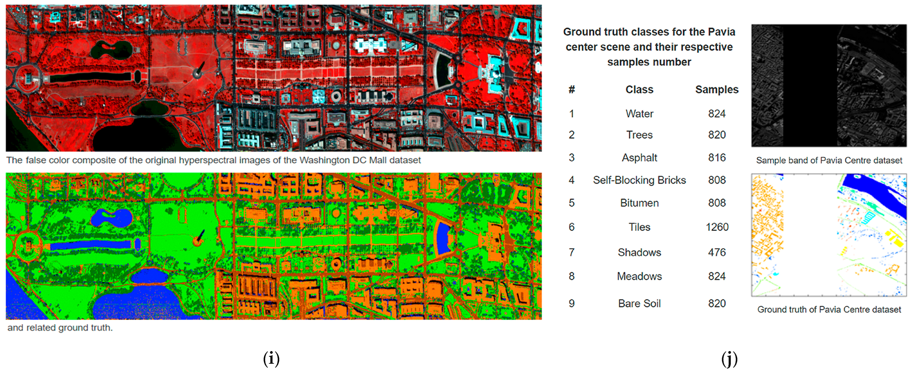
As regards the papers that analyzed the multispectral data, most of the authors chose to create the reference maps from the other images, whereas most of the authors that analyzed the hyperspectral data chose to employ the previous reference maps. It is important to emphasize that 97% of these reference maps are available online together with hyperspectral images and/or reference spectral libraries (e.g., [532,533,534,535] Figure 8). Therefore, these images were well known: Cuprite (NV, USA, e.g., [70,458]), Indian Pines (IN, USA, e.g., [78,458]), Jasper Ridge (CA, USA, e.g., [68,97]), Salinas Valley (CA, USA, e.g., [75,78]) datasets that were acquired with AVIRIS sensors; Pavia (Italy, e.g., [81,85]) datasets that were acquired with the ROSIS sensor; Samson (FL, USA, e.g., [59,89]) dataset that was acquired with the Samson sensor; University of Houston (TX, USA, e.g., [59,78]) dataset that was acquired with the CASI-1500 sensor; Urban (TX, USA, e.g., [59,68]) and Washington DC Mall (Washington, DC, USA, e.g., [81,90]) datasets that were acquired with the HYDICE sensor.
Moreover, 93% of these papers proposed a method and tested it not only on these “real” hyperspectral data, but also on created synthetic images. Borsoi et al. [4] highlighted that in order to overcome “the difficulty in collecting ground truth data”, some authors generated synthetic images. However, the authors complained because “there is not a clearly agreed-upon protocol to generate realistic synthetic data” [4].
3.4.4. Reference Fractional Abundance Maps
“Misclassifications” of the reference data or “misallocations of the reference data” are another possible source of error in spatial validation, defined as “imperfect reference data” by [519] or “error magnitude” by [518]. The authors highlighted that these errors can be caused also by the use of “standard” reference maps to validate the spectral unmixing results (i.e., the fractional abundance maps) [41,518,519]. The difference between standard reference maps and reference fractional abundance maps is that each pixel of the standard reference map is assigned to a corresponding land cover class, whereas each pixel of the reference fractional abundance map is labeled with the fractional abundances of each endmember that is present in that pixel. Therefore, the values of the standard reference map are equal to 0 or 1, whereas the values of the reference fractional abundance map are greater than 2 and vary between 0 and 1 (100 values are able to fully validate the fractional abundance of endmembers [114]).
The reference fractional abundance maps were employed by 133 eligible papers that were published in 2022, 2021, and 2020; by 62 eligible papers that were published in 2011 and 2010; and by 13 eligible papers that were published in 1996 and 1995 (45% of the total eligible papers). Moreover, among these works, 87, 47, and 8 papers estimated the full range of abundances using 100 values (31% of the total eligible papers), whereas 41, 10, and 5 works partially estimated the fractional abundances using less than 100 values (12% of the total eligible papers). It is important to note that 7% of the total eligible papers did not specify if they used the standard reference maps or the reference fractional abundance maps.
The eligible papers were separately analyzed according to reference data sources that were adopted in order to find out how fractional abundances were estimated. In the four parts of Figure 9, the eligible papers that were clustered according to the reference data sources are shown, and each part of Figure 9 shows the percentage of the papers that did not specify the reference maps used and the number of the papers that fully or partially estimated the reference fractional abundance maps.
High-spatial-resolution images were the most widely employed to make the reference fractional abundance maps (81% of the total papers that employed the images), followed by in situ data (68% of the total papers that employed in situ data), and then the maps (50% of the total papers that employed maps). Moreover, in situ data were the most widely employed to estimate the full range of fractional abundances (62% of the total papers that employed in situ data), followed by high-spatial-resolution images (52% of the total papers that employed the images), and then the maps (21% of the total papers that employed the images). The previous reference maps were not employed to make the reference fractional abundance maps.
Many authors highlighted that it is not easy to create the reference fractional abundances maps (e.g., [4,6,518,519]). Cavalli [145] implemented a method that was proposed by [537] in order to create the reference fractional abundance maps. This method is able to create the reference fractional abundance maps by varying the spatial resolution of the high-resolution reference maps several times, and the range of fractional abundances can be fully estimated according to the spatial resolution of the reference maps [114].
3.4.5. Validation of the Reference Data with Other Reference Data
In order to further minimize the errors due to “misclassifications” or “misallocations of the reference data” [518,519], some authors validated the reference data using other reference data: 61 eligible papers published in 2022, 2021, and 2020; 21 eligible papers published in 2011 and 2010; 4 eligible papers published in 1996 and 1995. Therefore, 81% of the total eligible papers did not take into consideration that the reference map may not be “ground truth” and may be “imperfect” [519,520].
It is very important to point out that some authors took advantage of the online availability of reference data to validate reference data (e.g., [114,123,127,140,145,152,231,448,496]). Many efforts are being made to create the networks of accurate validation data [48,538,539,540]. For example, Zhao et al. [140] exploited in situ measurements of the Leaf Area Index (LAI) that were provided by the VALERI project [540], whereas Halbgewachs et al. [123], Lu et al. [423], Shimabukuro et al. [353], and Tarazona Coronel [127] utilized validation data that were provided by the Program for Monitoring Deforestation in the Brazilian Amazon (PRODES) [541].
3.4.6. Error in Co-Localization and Spatial Resampling
The key issues described above addressed only the errors in the thematic accuracy of the spectral unmixing results [518,519], whereas this key issue aimed to address the geometric errors due to the comparison of remote images with reference data [542]. The impact of co-localization and spatial resampling errors was minimized and/or evaluated by 6% of the eligible papers: 20 eligible papers published in 2022, 2021, and 2020; 8 eligible papers published in 2011 and 2010; 1 eligible paper published in 1996. In order to minimized the errors, Arai et al. [368], Cao et al. [164], Li et al. [107], Soenen et al. [500], and Zurita-Milla et al. [419] carefully chose the size of the reference maps; Bair et al. [254], Cavalli [114,145], Ding et al. [152], Fernandez-Garcia et al. [256], Hamada et al. [441], Hajnal et al. [169], Lu et al. [435], Ma & Chan [78], Rittger et al. [262], Sun et al. [263], Yang et al. [488], and Yin et al. [151] spatially resampled the reference fractional abundance maps; Estes et al. [447] compared different windows of pixels (i.e., 3 × 3, 7 × 7, 11 × 11, 15 × 15, and 21 × 21); Pacheco & McNairn [480] selected the size and the spatial resolution of the reference maps; Ben-dor et al. [507], Fernandez-Guisuraga et al. [342], Kompella et al. [328], Laamarani et al. [343], and Plaza & Plaza [465] carefully co-localized the reference fractional abundance maps on the reference maps; Wang et al. [366] expanded the windows of the field sample size; Zhu et al. [64] resampled at “four kinds of grids” (i.e., 1100 × 1100 m, 2200 × 2200 m, 4400 × 4400 m, and 8800 × 8800 m) the reference fractional abundance map and compared the results. Bair et al. [254], Binh et al. [341], Cavalli [114,145], Cheng et al. [543], and Ruescas et al. [448] evaluated the errors in co-localization and spatial-resampling due to the comparison of different data at different spatial resolutions. Moreover, Cavalli [145] proposed a method to minimize the errors: the comparison of the histograms of the reference fractional abundance values with the histograms of the retrieved fractional abundance values.
It is important to point out that 94% of the total papers did not address the geometric errors due to the comparison of remote images with reference data.
4. Conclusions
The term validation is defined as “the process of assessing, by independent means, the quality of the data products derived from the system outputs” by the Working Group on Calibration and Validation (WGCV) of the Committee on Earth Observing Satellites (CEOS) [48]. Since 1969, research has been involved to establish shared key issues to validate the land cover products that were retrieved from the remote images [518,519,539,544]. These products can be obtained by applying classifications called “hard”, because they extract information only from “pure pixels,” and classifications called “soft”, because they also extract information from “mixed pixels” [519,544]. However, not only the literature related to the spatial validation, but also every review on the spectral unmixing procedure (i.e., a soft classification) highlighted that the key issues in the spatial validation of soft classification results have yet to be clearly established and shared (e.g., [4,6,518,519]).
Since no review was performed on this fundamental topic, this systematic review aims (a) to identify and analyze how the authors addressed the spatial validation of spectral unmixing results and (b) to provide readers with recommendations for overcoming the many shortcomings of spatial validation and minimizing its errors. The papers published in 2022, 2021, and 2020 were considered to analyze the current status of spatial validation, and the papers published not only in 2011 and 2010, but also in 1996 and 1995, were considered to analyze its progress over time. Since the literature on spectral unmixing is extensive, only papers published in these seven years were considered. A total of 454 eligible papers were included in this systematic review and showed that the authors addressed 6 key issues in the spatial validation. In this text, the order in which the key issues were presented is not an order of importance.
- The first key issue concerned the number of the endmembers validated. Some authors chose to focus on only one or two endmembers, and only these were spatially validated. This key issue was designed to facilitate the conduct of regional- or continental-scale studies and/or multitemporal analysis. It is important to note that 8% of the eligible papers did not specify which endmembers were validated.
- The second key issue concerned the sampling designs for the reference data. The authors who analyzed hyperspectral images preferred to validate the whole study area, whereas those who analyzed multispectral images preferred to validate small sample sizes that were randomly distributed. It is important to point out that 16% of the eligible papers did not specify the sampling designs for the reference data.
- The third key issue concerned the reference data sources. The authors who analyzed hyperspectral images primarily used the previously referenced maps and secondarily created reference maps using in situ data, whereas the authors who analyzed multispectral images chose to create reference maps primarily using high-spatial-resolution images and secondarily using in situ data.
- The fourth key issue was, perhaps, the one most closely related to the spectral unmixing procedure; it concerned the creation of the reference fractional abundance maps. Only 45% of the eligible papers created the reference fractional abundance maps to spatially validate the fractional abundance maps retrieved. These mainly employed high-resolution images and secondarily in situ data. Therefore, 55% of the eligible papers did not specify the employment of the reference fractional abundance maps.
- The fifth key issue concerned the validation of the reference data with other reference data; it was addressed only by 19% of the eligible papers. Therefore, 81% of the eligible papers did not validate the reference data.
- The sixth key issue concerned the error in co-localization and spatial resampling data, which was minimized and/or evaluated only by 6% of the eligible papers. Therefore, 94% of the eligible papers did not address the error in co-localization and spatial resampling data.
In conclusion, to spatially validate the spectral unmixing results and minimize and/or evaluate its errors, six key issues were considered not only from the eligible papers published in 2022, 2021 and 2020, but also from those published in 2010, 2011, 1996, and 1995. In addition, the results obtained from both hyperspectral and multispectral data were spatially validated considering all key issues, but these were addressed in different ways. All six key issues addressed together enabled rigorous spatial validation to be performed. Therefore, this systematic review provided readers with the most suitable tool to rigorously address spatial validation of the spectral unmixing results and minimize its errors.
The key difference between reference data suitable for hard and soft classifications is that the latter reference maps must have higher spatial resolution than the resolutions of the image pixels [6,114,518]. The optimal scale would be that 100 times larger than the image pixel resolution [114]. However, many hyperspectral data were validated using the previous reference maps at the same spatial resolution as the remote image, so these standard reference maps can only create reference fractional abundance maps with the help of other reference data. The employment of the standard reference maps instead of the reference fractional abundance maps was also evidenced by the employment of metrics to assess spatial accuracy that “assume implicitly that each of the testing samples is pure” [37,217].
However, only 4% of eligible papers addressed every key issue, and many authors did not specify which approach they employed to spatially validate the spectral unmixing results. Moreover, most of the authors who specified the approach employed did not adequately explain the methods used and the reasons for their choices. Six “good practice criteria to guide accuracy assessment methods and reporting” were identified by [519]. Therefore, these papers did not fully meet three good practice criteria: “reliable”, “transparent”, and “reproducible” [519].
Funding
This research received no external funding.
Data Availability Statement
Not applicable.
Conflicts of Interest
The authors declare no conflict of interest.
Appendix A
In accordance with the PRISMA statement [49,50], 454 eligible papers were identified, screened, and included in this systematic review: 326 eligible papers were published in 2022, 2021, and 2020; 112 eligible papers were published in 2011 and 2010; 16 eligible papers were published in 1996 and 1995. The eligible criterion was that the results of the spectral unmixing were spatially validated. Analyzing these papers, six key issues were identified that were differently addressed to spatially validate the spectral unmixing results. The different ways in which the key issues were addressed by the eligible papers published in 2022, 2021, 2020, 2011, 2010, 1996, and 1995 are summarized in Table A1, Table A2, Table A3, Table A4, Table A5, Table A6 and Table A7, respectively.
Table A1.
Main characteristics of the eligible papers that were published in 2022.
| Paper | Remote Image | Determined Endmembers | Validated Endmembers | Sources of Reference Data | Method for Mapping the Endmembers | Validation of Reference Data with Other Reference Data | Sample Sizes and Number of Small Sample Sizes | Sampling Designs | Reference Data | Estimation of Fractional Abundances | Error in Co-Localization and Spatial Resampling |
|---|---|---|---|---|---|---|---|---|---|---|---|
| Abay et al. [62] | ASTER (15–30 m) Landsat OLI (30 m) | Goethite, hematite | All | Geological map | - | In situ observations | - | - | Reference map | - | - |
| Ambarwulan et al. [147] | MERIS (300 m) | Several total suspended matter concentrations | All | In situ data | - | - | 171 samples | - | - | - | - |
| Benhalouche et al. [156] | PRISMA (30 m) | Hematite, magnetite, limonite, goethite, apatite | All | In situ data | - | - | - | - | - | - | - |
| Bera et al. [120] | Landsat TM, ETM+, OLI (30 m) | Vegetation, impervious surface, soil | All | Google Earth images | Photointerpretation | Soil map | 101 polygons | Uniform | Reference fractional abundance maps | Partial | - |
| Brice et al. [121] | Landsat TM, OLI (30 m) | Water, wetland vegetation, trees, grassland | 1 | Planet images (4 m) | Photointerpretation | In situ observations | 427 wetlands | - | Reference fractional abundance map | Partial | - |
| Cao et al. [164] | Sentinel-2 (10–20–60 m) | Vegetation, high albedo impervious surface, low albedo impervious surface, soil | All | GaoFen-2(0.8–3.8 m) | Photointerpretation | In situ observations | 300 squares (100 × 100 m) | Stratified random | Reference fractional abundance maps | Partial | Polygon size |
| Cavalli [114] | Hyperion (30 m) PRISMA (30 m) | Lateritic tiles, lead plates, asphalt, limestone, trachyte rock, grass, trees, lagoon water | All All | Panchromatic IKONOS image (1 m) Synthetic Hyperion and PRISMA images (0.30 m) | Photointerpretation The same spectral unmixing procedure performed to real images | In situ observations and shape files provided by the city and lagoon portal of Venice (Italy) | The whole study area | The whole study area | Reference fractional abundance maps | Full | Spatial resampling the reference maps and evaluation of the errors Evaluation of the errors in co-localization and spatial-resampling |
| Cavalli [145] | MIVIS (8m) | Lateritic tiles, lead plates, vegetation, asphalt, limestone, trachyte rock | All All | Panchromatic IKONOS image (1 m) Synthetic MIVIS image (0.30 m) | Photointerpretation The same spectral unmixing procedure performed to real image | In situ observations and shape files provided by the city and lagoon portal of Venice (Italy) | The whole study area | The whole study area | Reference fractional abundance maps | Partial | Spatial resampling the reference maps and evaluation of the errors Evaluation of the errors in co-localization and spatial-resampling |
| Cerra et al. [104] | DESIS (30 m) HySpex (0.6–1.2 m) Sentinel-2 (10–20–60 m) | PV panels, 2 grass, 2 forest, 2 soil, 2impervious surfaces | 1 | Reference map | - | - | The whole study area | The whole study area | - | - | - |
| Cipta et al. [137] | Landsat OLI (30 m) MODIS (500 m) | Rice, non-rice | All | In situ data | - | - | 10 samples | - | - | - | - |
| Compains Iso et al. [134] | Landsat TM, OLI (30 m) | Forest, shrubland, grassland, water, rock, bare soil | All | Orthophoto (≤ 0.5 m) | Photointerpretation | - | 50 squares (30 × 30 m) | Random | Reference fractional abundance maps | Partial | - |
| Damarjati et al. [157] | PRISMA (30 m) | A. obtusifolia, sand, wetland vegetations | All | In situ data | - | - | - | - | Reference maps | - | - |
| Dhaini et al. [70] | AVIRIS (20 m) | Andradite, chalcedony, kaolinite, jarosite, montmorillonite, nontronite Road, trees, water, soil Asphalt, dirt, tree, roof | All | Reference map | - | - | The whole study area | The whole study area | Reference maps | - | - |
| Ding et al. [122] | Landsat TM, OLI (30 m) | Vegetation, impervious surface, soil | All | Google satellite images (1 m) | Photointerpretation | - | 100 points | Random | Reference maps | - | - |
| Ding et al. [152] | MODIS (250–500 m) | Vegetation, non-vegetation | All | Landsat (30 m) | K-means unsupervised classified method | Google map | 5 Landsat images | Representative areas | Reference fractional abundance maps | Partial | Spatial resampling the reference maps |
| Fang et al. [71] | AVIRIS (20 m) | Road, 2building, trees, grass, soil Road, trees, water, soil | All | Reference map | - | - | The whole study area | The whole study area | Reference maps | - | - |
| Fernández-Guisuraga et al. [161] | Sentinel-2 (10–20 m) | Soil, green vegetation, non-photosynthetic vegetation | 1 | Photos | - | - | 60 situ plots (20 × 20 m) | Stratified random | Reference fractional abundance map | Full | - |
| Gu et al. [98] | AVIRIS (20 m) | Vegetation, soil, road, river soil, water, vegetation | All | Reference map | - | - | The whole study area | The whole study area | Reference maps | - | - |
| Guan et al. [86] | AVIRIS (20 m) | Trees, water, dirt, road | All | Reference map | - | - | The whole study area | The whole study area | Reference maps | - | - |
| HYDICE (10 m) | Asphalt, grass, trees, roofs | All | Reference map | - | - | The whole study area | The whole study area | Reference maps | - | - | |
| Hadi et al. [68] | AVIRIS (20 m) | Trees, water, dirt, road | All | Reference map | - | - | The whole study area | The whole study area | Reference maps | - | - |
| HYDICE (10 m) | Asphalt, grass, trees, roofs | All | Reference map | - | - | The whole study area | The whole study area | Reference maps | - | - | |
| Hajnal et al. [169] | Sentinel-2 (10–20–60 m) | Vegetation, impervious surface, soil | All | APEX image (2 m), High-resolution land cover map | Support vector classification | - | APEX image | Representative areas | Reference fractional abundance maps | Full | Spatial resampling the reference maps |
| Halbgewachs et al. [123] | Landsat TM, OLI (30 m), TIRS (60 m) | Forest, non-Forest (non-photosynthetic vegetation, soil, shade) | 2 | Annual classifications of the Program for Monitoring Deforestation in the Brazilian Amazon (PRODES) | - | Official truth-terrain data from deforested and non-deforested areas prepared by PRODES | 494 samples | Stratified random | Reference maps | - | - |
| He et al. [56] | AMMIS (0.5 m) | Urban surface materials | All | Reference map | - | - | The whole study area | The whole study area | Reference maps | - | - |
| ROSIS (4 m) | Urban surface materials | All | Reference map | - | - | The whole study area | The whole study area | Reference maps | - | - | |
| Hong et al. [69] | AVIRIS (20 m) | Trees, water, dirt, road, roofs | All | Reference map | - | - | The whole study area | The whole study area | Reference maps | - | - |
| EnMAP (30 m) | Asphalt, soil, water, vegetation | All | Reference map | - | - | The whole study area | The whole study area | Reference maps | - | - | |
| Hu et al. [149] | MODIS (0.5–1 km) | Blue ice, coarse-grained snow, fresh snow, bare rock, deep water, slush, wet snow | 1 | Sentinel-2 images | The same spectral unmixing procedure performed to MODIS images | Five auxiliary datasets | Six test areas identified as blue ice areas in the Landsat-based LIMA product | Representative areas | Reference fractional abundance maps | Full | - |
| Hua et al. [72] | AVIRIS (10 m) Samson (3.2 m) | Dirt, road - | All All | Reference map Reference map | - | - | The whole study area The whole study area | The whole study area The whole study area | Reference maps Reference maps | - | - |
| Jamshid Moghadam et al. [115] | Hyperion (30 m) | Kaolinite/smeetite, sepiolite, lizardite, chorite | All | Geological map | - | - | The whole study area | The whole study area | Reference maps | - | - |
| Jin et al. [143] | M3 hyperspectral image | Lunar surface materials | All | Lunar Soil Characterization Consortium dataset | - | - | - | - | Reference fractional abundance maps | Full | - |
| Jin et al. [73] | AVIRIS (10 m) Samson (3.2 m) | Road, soil, tree, water Water, tree, soil | All All | Reference map Reference map | - | - | The whole study area The whole study area | The whole study area The whole study area | Reference maps Reference maps | - | - |
| Kremezi et al. [166] | Sentinel-2 (10–20–60 m) WorldView-2 (0.46–1.8 m) WorldView-3 (0.31–1.24–3.7 m) | PET-1.5 l bottles, LDPE bags, fishing nets | All | In situ data | - | - | 3 squares (10 × 10 m) | - | Reference map | - | - |
| Kuester et al. [111] | HYDICE (10 m) | Urban surface materials | All | Reference map | - | - | The whole study area | The whole study area | Reference maps | - | - |
| Kumar et al. [113] | Hyperion (30 m) | Sal-forest, teak-plantation, scrub, grassland, water, cropland, mixed forest, urban, dry riverbed | All | Google Earth images | - | - | Same squares (30 × 30 m) | - | Reference fractional abundance maps | Partial | - |
| Lathrop et al. [124] | Landsat 8 OLI (15–30 m) | Mud, sandy mud, muddy sand, sand | All | In situ data | - | - | 805 circles (250 m radius) | Uniform | Reference fractional abundance map | Partial | - |
| Legleiter et al. [103] | DESIS (30 m) | 12 cyanobacteria genera, water | All | In situ data | - | - | - | - | - | - | - |
| Li et al. [75] | AVIRIS (10 m) | Vegetation, bare soil, vineyard, etc. | All | Field reference data | - | - | The whole study area | The whole study area | Reference maps | - | - |
| Hyperion (30 m) | - | All | Hyperion (30 m) image | - | - | The whole study area | The whole study area | Reference map | - | - | |
| Li et al. [74] | AVIRIS (10 m) | Tree, water, dirt, road | All | Reference map | - | - | The whole study area | The whole study area | Reference maps | - | - |
| Li et al. [107] | GaoFen-6 (2–8–16 m) Landsat 8 OLI (15–30 m) Sentinel-2 (10–20–60 m) | Green vegetation, bare rock, bare soil, non-photosynthetic vegetation | All | Photo acquired with drones | Classification | In situ measurements of fractional vegetation cover and bare rock | 285 polygons | Random | Reference fractional abundance maps | Full | Polygon size |
| Li et al. [76] | AVIRIS (10 m) | Andradite, chalcedony, kaolinite, jarosite, montmorillonite, nontronite | All | Reference map | - | - | The whole study area | The whole study area | Reference maps | - | - |
| HYDICE (10 m) | Asphalt, grass, trees, roofs | All | Reference map | - | - | The whole study area | The whole study area | Reference maps | - | - | |
| Luo et al. [77] | AVIRIS (10 m) | Andradite, chalcedony, kaolinite, jarosite, montmorillonite, nontronite | All | Reference map | - | - | The whole study area | The whole study area | Reference maps | - | - |
| HYDICE (10 m) | Asphalt, grass, trees, roofs | All | Reference map | - | - | The whole study area | The whole study area | Reference maps | - | - | |
| Lyngdoh et al. [100] | AVIRIS (20 m) AVIRIS-NG (5 m) | Trees, water, dirt, road Red soil, black soil, crop residue, built-up areas, bituminous roads, water | All | Reference map | - | - | The whole study area | The whole study area | Reference maps | - | - |
| Ma & Chang [78] | AVIRIS (10 m) | - | All | Reference map | - | - | The whole study area | The whole study area | Reference maps | - | Spatial resampling the reference maps |
| CASI (2.5 m) | Urban surface materials | All | Reference map | - | - | The whole study area | The whole study area | Reference maps | - | - | |
| ROSIS (4 m) | Urban surface materials | All | Reference map | - | - | The whole study area | The whole study area | Reference maps | - | - | |
| Matabishi et al. [469] | DESIS (30 m) | Roof materials | All | VHR images | - | Field validation data | 1053 ground reference points | - | Reference fractional abundance maps | Full | - |
| Meng et al. [163] | Sentinel-2 (10–20–60 m) | Vegetation, non-vegetation | 1 | Google Earth Pro image (1 m) | - | - | 10535 squares (10 × 10 m) | Stratified random | Reference fractional abundance maps | Partial | - |
| Nill et al. [125] | Landsat TM, OLI (30 m) | Shrubs, coniferous trees, herbaceous plants, lichens, water, barren surfaces | All | RGB camera (0.4–8 cm) Orthophotos (10–15 cm) | - | Field validation data | 216 validation pixels | Stratified random | Reference fractional abundance maps | Full | - |
| Ouyang et al. [126] | Landsat-8 OLI (30 m) | Impervious surface, evergreen vegetation, seasonally exposed soil | 1 | Land use and land cover maps (0.5 m) | - | - | 264 circles (1 km radius) | Random | Reference fractional abundance map | Partial | - |
| Ozer & Leloglu [167] | Sentinel-2 (10–20–60 m) | Soil, vegetation, water | All | Aerial images (30 cm) | - | - | - | - | Reference fractional abundance map | Partial | - |
| P et al. [61] | ASTER (90 m) | Iron Oxide | 1 | In situ data | - | - | 13 samples | - | - | - | - |
| Palsson et al. [59] | Apex | Asphalt, vegetation, water, roof | All | Reference map | - | - | The whole study area | The whole study area | Reference maps | - | - |
| AVIRIS (10 m) | Road, soil, tree, water | All | Reference map | - | - | The whole study area | The whole study area | Reference maps | - | - | |
| CASI (2.5) | Urban surface materials | All | Reference map | - | - | The whole study area | The whole study area | Reference maps | - | - | |
| HYDICE (10 m) | Asphalt, grass, trees, roofs | All | Reference map | - | - | The whole study area | The whole study area | Reference maps | - | - | |
| Samson (3.2 m) | Soil, tree, water | All | Reference map | - | - | The whole study area | The whole study area | Reference maps | - | - | |
| Pan & Jiang [65] | AVHRR (1–5 km) | Snow, bare land, grass, forest, shadow | All | Landsat7 TM+ image (30 m) | The same procedure performed to AVHRR image | - | Landsat image | Representative area | Reference fractional abundance maps | Full | - |
| Pan et al. [66] | AVHRR (1–5 km) | Snow, bare land, grass, forest, shadow | All | Landsat5 TM image (30 m) | The same procedure performed to AVHRR image | The land use/land cover | Landsat image | Representative area | Reference fractional abundance maps | Full | - |
| Paul et al. [470] | DESIS (30 m) | PV panel, vegetation, sand | All | VHR image | - | - | - | Random | Reference fractional abundance maps | Full | - |
| Pervin et al. [154] | NEON (1 m) | Tall woody plants, herbaceous and low stature vegetation, bare soil | All | NEON AOP image (0.1 m) | Supervised classification | Drone imagery (0.01 m) | 13 sets of 10 pixels | Random | Reference fractional abundance maps | Partial | - |
| Qi et al. [89] | AVIRIS (10 m) | Road, soil, tree, water | All | Reference map | - | - | The whole study area | The whole study area | Reference maps | - | - |
| HYDICE (10 m) | Asphalt, grass, trees, roofs | All | Reference map | - | - | The whole study area | The whole study area | Reference maps | - | - | |
| Samson (3.2 m) | Soil, tree, water | All | Reference map | - | - | The whole study area | The whole study area | Reference maps | - | - | |
| Rajendran et al. [116] | Hyperion (30 m) | Chlorophyll-a | 1 | WorldView-3 image (0.31–1.24–3.7 m) | Field validation data | - | - | Reference fractional abundance maps | Full | - | |
| Ronay et al. [170] | Specim IQ | Weed species | All | In situ data | - | - | The whole study area | The whole study area | Reference fractional abundance maps | Full | - |
| Santos et al. [131] | Landsat MSS, TM, OLI (30 m) | Natural vegetation, anthropized area, burned, water | All | In situ data | - | - | samples | Random | Reference maps | - | - |
| Shaik et al. [158] | PRISMA (30 m) | Broadleaved forest, Coniferous forest, Mixed forest, Natural grasslands, Sclerophyllous vegetation | All | Land use and land cover map | - | Field validation data | - | - | Reference maps | - | - |
| Shao et al. [109] | Landsat-8 OLI (15–30 m) GaoFen-1 (2–8–16 m) | Vegetation, soil impervious surfaces (high albedo; low albedo), water | 1 | GaoFen-1 image (2 m) | Object-based classification and photointerpretation of the results. | Ground-based measurements | 300 pixels | Uniform | Reference fractional abundance map | Partial | - |
| Shi et al. [90] | AVIRIS (10 m) | Road, soil, tree, water | All | Reference map | - | - | The whole study area | The whole study area | Reference maps | - | - |
| HYDICE (10 m) | Road, roof, soil, grass, trail, tree, water | All | Reference map | - | - | The whole study area | The whole study area | Reference maps | - | - | |
| Shi et al. [79] | AVIRIS (10 m) | Road, soil, tree, water | All | Reference map | - | - | The whole study area | The whole study area | Reference maps | - | - |
| HYDICE (10 m) | Road, roof, soil, grass, trail, tree, water | All | Reference map | - | - | The whole study area | The whole study area | Reference maps | - | - | |
| Shimabukuro et al. [132] | Landsat TM, OLI (30 m) | Forest plantation | All | MapBiomas annual LULC map collection 6.0 | - | - | 20000 samples | Stratified random | Reference maps | Partial | - |
| Silvan-Cardenas et al. [139] | Landsat (30 m) | - | - | In situ data | - | - | samples | - | Reference maps | - | - |
| Sofan et al. [135] | Landsat-8 OLI (15–30 m) | Vegetation, smoldering, burnt area | All | PlanetScope images (3 m) | Photointerpretation | - | - | Random | - | - | - |
| Song et al. [153] | MODIS (0.5 km) | Water, urban, tree, grass | All | GlobalLand30 maps (GLC30) produced based on Landsat (30 m) | - | - | - | - | Reference fractional abundance maps | Full | - |
| AVIRIS (10 m) | - | - | Reference map | - | - | The whole study area | The whole study area | Reference maps | - | - | |
| HYDICE (10 m) | Road, roof, soil, grass, trail, tree, water | - | Reference map | - | - | The whole study area | The whole study area | Reference maps | - | - | |
| Sun et al. [80] | AVIRIS (10 m) | Andradite, chalcedony, kaolinite, jarosite, montmorillonite, nontronite | All | Reference map | - | - | The whole study area | The whole study area | Reference fractional abundance maps | Full | - |
| Sun et al. [165] | Sentinel-2 (10–20–60 m) | Rice residues, soil, green moss, white moss | 1 | Photos (1.5 m) | Photointerpretation | In situ observations | 30 samples | Random | Reference fractional abundance maps | Partial | - |
| Sutton et al. [119] | Landsat TM, OLI (30 m) | Drylands, semi-arid zone, arid zone | All | In situ data | - | - | 4207 samples | No-uniform | - | - | - |
| Tao et al. [91] | AVIRIS (10 m) | Andradite, chalcedony, kaolinite, jarosite, montmorillonite, nontronite | All | Reference map | - | - | The whole study area | The whole study area | Reference maps | - | - |
| Tarazona Coronel [127] | Landsat TM, OLI (30 m) | Vegetation | 1 | Landsat (15–30 m) and Sentinel-2 (10–20–60 m) images | Photointerpretation | Official truth-terrain data from deforested and non-deforested areas prepared by PRODES | 300 samples | Stratified random | Reference fractional abundance maps | Partial | - |
| van Kuik et al. [133] | Landsat TM, OLI (30 m) Sentinel-2 (10–20–60 m) | Blowouts to sand, water, vegetation | 1 | Unoccupied Aerial Vehicle (UAV) orthomosaics (1 m) | Photointerpretation | - | - | - | Reference fractional abundance maps | Partial | - |
| Viana-Soto et al. [138] | Landsat TM, OLI (30 m) | Tree, shrub, background (herbaceous, soil, rock) | 1 | Orthophotos | Photointerpretation | Validation samples | - | Uniform | Reference fractional abundance maps | Full | - |
| Wang et al. [87] | AVIRIS (10 m) | - | - | Reference map | - | - | The whole study area | The whole study area | Reference maps | - | - |
| Wang et al. [142] | Landsat-8 OLI (30 m) | Impervious surfaces (high albedo, low albedo), forest, grassland, soil | 1 | QuickBird image (0.6 m) | Spectral angle mapping classification | In situ observations | 13,080 points | Random | Reference fractional abundance maps | Partial | - |
| Wang et al. [150] | MODIS (0.5 km) | Vegetation, non-vegetation | All | Landsat image (30 m) | K-means-based unsupervised classification | - | Landsat image | Representative area | Reference fractional abundance maps | Partial | - |
| Wang et al. [92] | AVIRIS (10 m) | Andradite, chalcedony, kaolinite, jarosite, montmorillonite, nontronite | All | Reference map | - | - | The whole study area | The whole study area | Reference map | - | - |
| Wu & Wang [85] | AVIRIS (10 m) | Urban surface materials | All | Reference map | - | - | The whole study area | The whole study area | Reference maps | - | - |
| HYDICE (10 m) | Road, roof, soil, grass, trail, tree, water | All | Reference map | - | - | The whole study area | The whole study area | Reference maps | - | - | |
| ROSIS (4 m) | Urban surface materials | All | Reference map | - | - | The whole study area | The whole study area | Reference maps | - | - | |
| Xia et al. [128] | Landsat ETM+, OLI (30 m) | High albedo, vegetation low albedo, shadow | 2 | Google Earth images | Photointerpretation | - | 100 polygons (30 × 30 m) | Random | Reference fractional abundance maps | Partial | - |
| Xu et al. [162] | Sentinel-2 (10–20–60 m) | Impervious surface, water body, vegetation, bare land | All | Google Earth images | Photointerpretation | In situ observations | - | - | Reference fractional abundance maps | Partial | - |
| Yang et al. [57] | AMMIS (0.5 m) AVIRIS ROSIS | - | All | Reference map | - | - | The whole study area | The whole study area | Reference maps | - | - |
| Yang [81] | AVIRIS (20 m) | Vegetation, water, soil | All | Reference map | - | - | The whole study area | The whole study area | Reference maps | - | - |
| HYDICE (10 m) | Road, roof, soil, grass, trail, tree, water | All | Reference map | - | - | The whole study area | The whole study area | Reference maps | - | - | |
| ROSIS (4 m) | Urban surface materials | All | Reference map | - | - | The whole study area | The whole study area | Reference maps | - | - | |
| Yang et al. [141] | Landsat-8 OLI (30 m) | Water, non-water | All | Google Earth images | - | - | The whole study area | The whole study area | Reference fractional abundance maps | Partial | - |
| Yi et al. [82] | AVIRIS (20 m) | Vegetation, water, soil | All | Reference map | - | - | The whole study area | The whole study area | Reference maps | - | - |
| HYDICE (10 m) | Road, roof, soil, grass, trail, tree, water | All | Reference map | - | - | The whole study area | The whole study area | Reference maps | - | - | |
| Yin et al. [82] | MODIS (0.250 km) | Water, soil | 1 | Landsat OLI image (30 m) | Modified normalized difference water index (MNDWI) | - | Landsat image | Representative area | Reference fractional abundance maps | Partial | Spatial resampling the reference maps |
| Zhang & Jiang [108] | Landsat (30 m) Sentinel-2 (20 m) MODIS (0.5 km) | Snow | 1 | GaoFen-2 image (3.2 m) | Supervised classification | - | - | - | Reference fractional abundance map | Partial | - |
| Zhang et al. [117] | HySpec (0.7 m) | Bitumen, red-painted metal sheets, blue fabric, red fabric, green fabric, grass | All | Reference map | - | - | - | - | Reference maps | Partial | - |
| Zhang et al. [83] | AVIRIS (20 m) | Andradite, chalcedony, kaolinite, jarosite, montmorillonite, nontronite | All | Reference map | - | - | The whole study area | The whole study area | Reference maps | - | - |
| Zhang et al. [93] | AVIRIS (10/20 m) | Dumortierite, muscovite, Alunite+muscovite, kaolinite, alunite, montmorillonite Tree, water, road, soil | All | Reference map | - | - | The whole study area | The whole study area | Reference maps | - | - |
| Zhang et al. [129] | Landsat-8 OLI (30 m) | Vegetation, impervious surfaces | All | GaoFen-1 image (2–8 m) | Photointerpretation | - | 101 samples | Uniform | Reference fractional abundance maps | Partial | - |
| Zhang et al. [130] | Landsat-8 OLI (30 m) | Vegetation | All | GaoFen-1 image (2–8 m) | Object-based classification | - | 101 samples | Uniform | Reference fractional abundance map | Partial | - |
| Zhang et al. [88] | AVIRIS (10/20 m) | Cuprite, road, trees, water, soil Asphalt, dirt, tree, roof | All | Reference map Reference map | - | - | The whole study area | The whole study area | Reference maps | - | - |
| Zhao et al. [84] | AVIRIS (10 m) | Road, trees, water, soil Asphalt, grass, tree, roof, metal, dirt | All | Reference map Reference map | - | - | The whole study area | The whole study area | Reference maps | - | - |
| Zhao et al. [96] | AVIRIS (10 m) | Road, trees, water, soil | All | Reference map | - | - | The whole study area | The whole study area | Reference maps | - | - |
| HYDICE (10 m) | Road, roof, soil, grass, trail, tree, water | All | Reference map | - | - | The whole study area | The whole study area | Reference maps | - | - | |
| Zhao et al. [94] | AVIRIS (10 m) | Road, trees, water, soil | All | Reference map | - | - | The whole study area | The whole study area | Reference maps | - | - |
| Zhao et al. [95] | AVIRIS (20 m) | Andradite, chalcedony, kaolinite, jarosite, montmorillonite, nontronite | All | Reference map | - | - | The whole study area | The whole study area | Reference maps | - | - |
| Zhao et al. [136] | Landsat-8 OLI (30 m) Sentinel-2 (10–20–60 m) | Impervious surfaces, vegetation, soil, water | 2 | WorldView-2 image (0.50–2 m) | - | - | 172 polygons (480 × 480 m) | Random | Reference fractional abundance maps | Full | - |
| Zhao et al. [140] | Landsat (30 m) Spot (30 m) | Vegetation | 1 | Fractional vegetation cover reference maps (provided by VALERI project and the ImagineS) | - | In situ measurements of LAI (provided by VALERI project and the ImagineS) | 445 squares (20 × 20 m or 30 × 30 m) | - | Reference fractional abundance map | Full | - |
| Zhao & Qin [168] | Sentinel-2 (10–20–60 m) | Vegetation, mineral area | All | In situ data | - | - | - | - | Reference fractional abundance maps | Partial | - |
| Zhu et al. [64] | AVHRR (1–5 km) | Snow, non-snow (bare land, vegetation, and water) | 1 | Landsat TM image (30 m) | Normalized difference snow index | - | Landsat image | Representative area | Reference fractional abundance map | Full | Spatial resolution variation |
| Zhu et al. [97] | AVIRIS (10 m) | Road, trees, water, soil | All | Reference map | - | - | The whole study area | The whole study area | Reference maps | - | - |
| HYDICE (10 m) | Road, roof, soil, grass, trail, tree, water | All | Reference map | - | - | The whole study area | The whole study area | Reference maps | - | - | |
| Samson (3.2 m) | Soil, tree, water | All | Reference map | - | - | The whole study area | The whole study area | Reference maps | - | - |
Table A2.
Main characteristics of the eligible papers that were published in 2021.
| Paper | Remote Image | Determined Endmembers | Validated Endmembers | Sources of Reference Data | Method for Mapping the Endmembers | Validation of Reference Data with Other Reference Data | Sample Sizes and Number of Small Sample Sizes | Sampling Designs | Reference Data | Estimation of Fractional Abundances | Error in Co-Localization and Spatial Resampling |
|---|---|---|---|---|---|---|---|---|---|---|---|
| Azar et al. [174] | AVIRIS CASI | Trees, Mostly Grass Ground Surface, Mixed Ground Surface, Dirt/Sand, Road | All All | Reference map CASI image | - Photointerpretation | - | The whole study area | The whole study area | Reference map Reference map | - | - |
| Badola et al. [226] | AVIRIS-NG (5 m) Sentinel-2 (10–20–60 m) | Black Spruce Birch Alder Gravel | All | In situ data | Photointerpretation | In situ observations | 29 plots | Random | Reference map | - | - |
| Bai et al. [175] | AVIRIS | Asphalt, Grass, Tree, Roof, Metal, Dirt | All | Reference map | - | - | The whole study area | The whole study area | Reference map | - | - |
| Bair et al. [254] | Landsat MODIS | Snow, canopy | 1 | WorldView-2–3 images (0.34–0.55 m) | Photointerpretation | Airborne Snow Observatory (ASO) (3 m) | - | - | Reference fractional abundance map | Full | Spatial resampling the reference maps Evaluation of the errors in co-localization and spatial-resampling |
| Benhalouche et al. [230] | HYDICE (10 m) Samson (3.2) | Asphalt, grass, tree, roof Soil, tree, water | All | Reference map | - | - | The whole study area | The whole study area | Reference map | - | - |
| Benhalouche et al. [265] | PRISMA (30 m) | Mineral | All | Geological map | - | - | The whole study area | The whole study area | Reference map | - | - |
| Borsoi et al. [176] | AVIRIS | - | All | Reference map | - | - | The whole study area | The whole study area | Reference map | - | - |
| Cerra et al. [238] | HySpex | Target | All | In situ data | - | Reference targets and Aeronet data | - | - | Reference fractional abundance maps | - | - |
| Chang et al. [229] | GF-5 (30 m) Sentinel 2 (10–20–60 m) ZY-1-02D (30 m) | - | All | In situ data | - | - | - | - | Reference fractional abundance maps | - | - |
| Chen et al. [239] | Landsat | - | All | UAV images | - | Ground survey data | - | - | Reference fractional abundance maps | - | - |
| Chen et al. [245] | Landsat | Vegetation, impervious surface, bare soil, and water | All | Google Earth images | - | - | - | - | Reference fractional abundance maps | - | - |
| Chen et al. [246] | Landsat | - | All | Google Earth images | - | Field surveys | 300 plots | Random | Reference fractional abundance maps | - | - |
| Converse et al. [247] | Landsat | Green vegetation, non-photosynthetic vegetation, soil | All | UAS images | - | Field surveys | Plots | - | Reference fractional abundance maps | Full | - |
| Di et al. [177] | AVIRIS | Cuprite | All | Reference map | - | - | The whole study area | The whole study area | Reference map | - | - |
| Dong & Yuan [178] | AVIRIS | - | All | Reference map | - | - | The whole study area | The whole study area | Reference map | - | - |
| Dong et al. [179] | AVIRIS | - | All | Reference map | - | - | The whole study area | The whole study area | Reference map | - | - |
| Dong et al. [180] | AVIRIS | - | All | Reference map | - | - | The whole study area | The whole study area | Reference map | - | - |
| Dutta et al. [248] | Landsat | Vegetation, impervious surface, bare soil, | 1 | In situ data | - | Built-up density, urban expansion and population density of the area | - | - | Reference fractional abundance maps | Full | - |
| Ekanayake et al. [181] | AVIRIS | - | All | Reference map | - | - | The whole study area | The whole study area | Reference map | - | - |
| Elrewainy & Sherif [182] | AVIRIS | - | All | Reference map | - | - | The whole study area | The whole study area | Reference map | - | - |
| Feng & Fan [255] | Landsat (30 m) Sentinel 2 (10–20–60 m) | Vegetation, high-albedo impervious surface, low-albedo impervious surface soil | All | In situ data | - | - | 18000 testing areas | random | Reference fractional abundance maps | Full | - |
| Fernández-García et al. [256] | Landsat (30 m) | Arboreal vegetation, shrubby vegetation, herbaceous vegetation, rock and bare soil, water | All | Orthophotographs (0.25 m) | - | - | 250 plots (30 × 30 m) | random | Reference fractional abundance maps | Full | Spatial resolution variation |
| Finger et al. [249] | Landsat (30 m) | - | All | California Department of Fish and Wildlife (CDFW) aerial survey canopy area product | - | - | - | - | Reference fractional abundance maps | Full | - |
| Gu et al. [183] | AVIRIS | - | All | Reference map | - | - | The whole study area | The whole study area | Reference map | - | - |
| Guo et al. [184] | AVIRIS | - | All | Reference map | - | - | The whole study area | The whole study area | Reference map | - | - |
| Gu et al. [185] | AVIRIS | - | All | Reference map | - | - | The whole study area | The whole study area | Reference map | - | - |
| Han et al. [186] | AVIRIS | Asphalt, grass, tree, roof | All | Reference map | - | - | The whole study area | The whole study area | Reference map | - | - |
| Han et al. [268] | AVIRIS | - | All | Reference map | - | - | The whole study area | The whole study area | Reference map | - | - |
| Haq et al. [234] | Hyperion (30 m) | Clean snow, blue ice, refreezing ice dirty snow, dirty glacier ice, firn, moraine, and glacier ice | All | In situ data | - | Sentinel-2 images | - | - | Reference fractional abundance maps | Full | - |
| He et al. [231] | HYDICE (10 m) MODIS (0.5–1 km) | - | All All | Reference map Finer Resolution Observation and Monitoring of Global Land Cov (30 m) | - | - | - 61 scenes | - | Reference fractional abundance maps | Full | - |
| He et al. [56] | ROSIS (4m) | Urban surface materials | All | Reference map | - | - | The whole study area | The whole study area | Reference map | - | - |
| Hua et al. [187] | AVIRIS | - | All | Reference map | - | - | The whole study area | The whole study area | Reference map | - | - |
| Hua et al. [188] | AVIRIS Samson (3.2) | - Soil, tree, water | All | Reference map | - | - | The whole study area | The whole study area | Reference map | - | - |
| Huang et al. [189] | AVIRIS | - | All | Reference map | - | - | The whole study area | The whole study area | Reference map | - | - |
| Jia et al. [190] | AVIRIS | Cuprite | All | Reference map | - | - | The whole study area | The whole study area | Reference map | - | - |
| Ji et al. [235] | Hyperion (30 m) | Photosynthetic vegetation, non-photosynthetic vegetation, bore soil | All | Reference map | - | - | The whole study area | The whole study area | Reference map | - | - |
| Jiji [250] | Landsat (30 m) | Heavy metals | All | In situ data | - | - | 17 samples | Random | Reference fractional abundance maps | Full | - |
| Jin et al. [267] | ROSIS (4 m) Samson (3.2 m) | Urban surface materials Soil, tree, water | All | Reference map | - | - | The whole study area | The whole study area | Reference map | - | - |
| Kneib et al. [271] | Sentinel 2 (10–20–60 m) | - | all | Pleiades images (2 m) | Photointerpretation | - | - | - | Reference fractional abundance maps | Full | - |
| Kucuk & Yuksel [202] | AVIRIS | Cuprite | All | Reference map | - | - | The whole study area | The whole study area | Reference map | - | - |
| Kumar & Chakravortty [191] | AVIRIS ROSIS (4 m) | - Urban surface materials | All | Reference map | - | - | The whole study area | The whole study area | Reference map | - | - |
| Li et al. [203] | AVIRIS | Cuprite | All | Reference map | - | - | The whole study area | The whole study area | Reference map | - | - |
| Li et al. [192] | AVIRIS HYDICE (10 m) | Cuprite - | All | Reference map | - | - | The whole study area | The whole study area | Reference map | - | - |
| Li et al. [193] | AVIRIS | All | Reference map | - | - | The whole study area | The whole study area | Reference map | - | - | |
| Li [194] | AVIRIS | Cuprite | All | Reference map | - | - | The whole study area | The whole study area | Reference map | - | - |
| Li et al. [195] | AVIRIS | Cuprite | All | Reference map | - | - | The whole study area | The whole study area | Reference map | - | - |
| Li et al. [196] | AVIRIS | Cuprite | All | Reference map | - | - | The whole study area | The whole study area | Reference map | - | - |
| Li et al. [197] | AVIRIS | Cuprite | All | Reference map | - | - | The whole study area | The whole study area | Reference map | - | - |
| Li et al. [251] | Landsat (30 m) | Impervious, vegetation, bare land, water | All | Google Earth images | - | Field surveys | 4296 sampled points | Random | Reference fractional abundance maps | Full | - |
| Li [257] | Landsat (30 m) | Impervious, soil, vegetation | All | Images | - | - | 200 sample points | Random | Reference fractional abundance maps | Full | - |
| Li et al. [204] | AVIRIS HYDICE (10 m) | - | All | Reference map | - | - | The whole study area | The whole study area | Reference map | - | - |
| Li et al. [205] | AVIRIS | Cuprite | All | Reference map | - | - | The whole study area | The whole study area | Reference map | - | - |
| Liu et al. [206] | AVIRIS | - | All | Reference map | - | - | The whole study area | The whole study area | Reference map | - | - |
| Lui & Zhu [207] | AVIRIS Samson (3.2 m) | - Soil, tree, water | All | Reference map | - | - | The whole study area | The whole study area | Reference map | - | - |
| Lombard & Andrieu [240] | Landsat | - | 3 | Google Earth images | Phointerpretation | - | 8490 sample points | Random | Reference fractional abundance maps | Full | - |
| Luo & Chen [260] | Landsat | Vegetation, impervious, soil | 1 | Gaofen-2 and WorldView-2 images | - | - | - | - | Reference fractional abundance maps | Full | Spatial resolution variation |
| Ma et al. [276] | WorldView-3 | Vegetation | All | Digital cover photography | - | Vegetation spectra | 30 sample points | - | Reference fractional abundance map | Full | - |
| Mudereri et al. [273] | Sentinel 2 (10–20–60 m) | - | All | Google Earth images | - | Field surveys | 1370 pixels | Random | Reference fractional abundance maps | Full | - |
| Muhuri et al. [258] | Landsat Sentinel 2 (10–20–60 m) | Snow cover | All | In situ data | - | Airborne Snow Observatory (ASO) (2 m) | - | - | Reference fractional abundance maps | Full | - |
| Okujeni et al. [228] | Simulated EnMAP | - | All | Google Earth images | - | Landsat images | 3183 sites | Random | Reference fractional abundance maps | Full | - |
| Ou et al. [233] | HyMap (4.5 m) | Soil organic matter, soil heavy meta | All | In situ data | - | - | 95 soil samples | Random | Reference fractional abundance maps | Full | - |
| Pan et al. [261] | MODIS (0.5–1 km) | Snow | All | Landsat images | MESMA | - | The whole study area | The whole study area | Reference fractional abundance maps | Full | - |
| Patel et al. [208] | AVIRIS | - | All | Reference map | - | - | The whole study area | The whole study area | Reference map | - | - |
| Peng et al. [209] | AVIRIS | - | All | Reference map | - | - | The whole study area | The whole study area | Reference map | - | - |
| Qin et al. [210] | AVIRIS Samson (3.2 m) | - Soil, tree, water | All | Reference map | - | - | The whole study area | The whole study area | Reference map | - | - |
| Racoviteanu et al. [241] | Landsat | Debris-covered glaciers | All | Pléiades 1A image (2 m) RapidEye image (5 m) PlanetScope (3 m) | Phointerpretation | DEM | 151 test pixels | Random | Reference fractional abundance maps | Full | - |
| Rittger et al. [262] | MODIS (0.5–1 km) | Snow | All | Landsat images | - | - | - | Random | Reference fractional abundance maps | Full | Spatial resolution variation |
| Sall et al. [252] | Landsat (30 m) | Waterbodies | All | DigitalGlobe WorldView-2 (0.46 m) | - | National AgricultureImagery Program (NAIP) | - | - | Reference fractional abundance maps | Full | - |
| Sarkar & Sur [173] | ASTER (15–30–90 m) | Bauxite minerals | All | In situ data | - | Petrological, EPMA, SEM-EDS studies DEM | - | - | Reference fractional abundance maps | Full | - |
| Seydi & Hasanlou [236] | Hyperion (30 m) | - | All | In situ data | - | - | 73505 samples | Random | Reference fractional abundance maps | Full | - |
| Seydi & Hasanlou [237] | Hyperion (30 m) | - | All | In situ data | - | - | - | - | Reference fractional abundance maps | Full | - |
| Shahid & Schizas [211] | AVIRIS Samson (3.2 m) | - Soil, tree, water | All | Reference map | - | - | The whole study area | The whole study area | Reference map | - | - |
| Shen et al. [242] | Landsat (30 m) | Impervious, non-impervious surface | All | Land use map by the National Basic Geographic Information Center | - | - | - | - | Reference map | - | - |
| Shen et al. [270] | Sentinel 2 (10–20–60 m) | - | All | Google Earth images | Phointerpretation | - | 467 polygons | Random | Reference fractional abundance maps | Full | - |
| Shumack et al. [243] | Landsat (30 m) Sentinel 2 (10–20–60 m) | Bare soil, photosynthetic vegetation, non-photosynthetic vegetation | All | Orthorectified mosaic images (0.02 m) | Object based image analyses | SLATS dataset of fractional ground cover surveys | 400 point per images | Random | Reference fractional abundance maps | Full | - |
| Song et al. [232] | HYDICE (10 m) Samson (3.2 m) | Road, trees, water, soil Soil, tree, water | All | Reference map | - | - | The whole study area | The whole study area | Reference map | - | - |
| Soydan et al. [272] | Sentinel 2 (10–20–60 m) | - | All | Laboratory analysis of field collected samples through Inductive Coupled Plasma | - | Laboratory analysis of field collected samples through X-Ray Diffraction, and ASD spectral analysis | - | - | Reference fractional abundance maps | Full | - |
| Su et al. [212] | AVIRIS HYDICE (10 m) Hyperion (30 m) | - Road, trees, water, soil | All | Reference map | - | - | The whole study area | The whole study area | Reference map | - | - |
| Sun et al. [263] | MODIS (0.5–1 km) | Green vegetation, sand, saline, and dark surface | All | Google Earth images Field observations | - | - | 89 samples 10 plots (1 × 1 km) | Random | Reference fractional abundance maps | Full | Spatial resolution variation |
| Sun et al. [275] | WorldView-2 | Mosses, lichens, rock, water, snow | In situ data | - | Photos and spectra | 32 plots (2 × 2 m) | Random | Reference fractional abundance maps | - | - | |
| Tan et al. [198] | AVIRIS | Cuprite | All | Reference map | - | - | The whole study area | The whole study area | Reference map | - | - |
| Vibhute et al. [213] | AVIRIS | Tree, soil, water, road | All | Reference map | - | - | The whole study area | The whole study area | Reference map | - | - |
| Wan et al. [214] | AVIRIS HYDICE (10 m) Samson (3.2 m) | - Soil, tree, water | All | Reference map | - | - | The whole study area | The whole study area | Reference map | - | - |
| Wang et al. [215] | AVIRIS | - | All | Reference map | - | - | The whole study area | The whole study area | Reference map | - | - |
| Vermeulen et al. [244] | Landasat Sentinel 2 (10–20–60 m) | Soil, Photosynthetic Vegetation, Non-Photosynthetic Vegetation | All | Images, field data | - | - | (10 × 10 m) plots | - | Reference fractional abundance maps | - | - |
| Wang et al. [199] | AVIRIS | - | All | Reference map | - | - | The whole study area | The whole study area | Reference map | - | - |
| Wang et al. [216] | AVIRIS HYDICE (10 m) | - | All | Reference map | - | - | The whole study area | The whole study area | Reference map | - | - |
| Wang [217] | AVIRIS ROSIS (4 m) | - Urban surface materials | All | Reference map | - | - | The whole study area | The whole study area | Reference map | - | - |
| Wang et al. [200] | AVIRIS ROSIS (4 m) | - Urban surface materials | All | Reference map | - | - | The whole study area | The whole study area | Reference map | - | - |
| Wu et al. [253] | Landsat Sentinel 2 (10–20–60 m) | Bare soil, agricultural crop Water, vegetation, urban | All | Google Maps | Phointerpretation | - | - | - | Reference fractional abundance maps | Full | - |
| Xiong et al. [201] | AVIRIS | - | All | Reference map | - | - | The whole study area | The whole study area | Reference map | - | - |
| Xiong et al. [218] | AVIRIS HYDICE (10 m) | - Road, trees, water, soil | All | Reference map | - | - | The whole study area | The whole study area | Reference map | - | - |
| Xu et al. [219] | AVIRIS | Cuprite | All | Reference map | - | - | The whole study area | The whole study area | Reference map | - | - |
| Xu & Somers [269] | Sentinel 2 (10–20–60 m) | Vegetation, soil, impervious surface | All | Google Earth images | Object-oriented classification | - | - | - | Reference fractional abundance maps | Full | - |
| Yang et al. [264] | MODIS (0.5–1 km) | Vegetation, soil | All | GF-1, Google Earth images | - | - | 2044 samples (0.5 × 0.5 km) | Random | Reference fractional abundance maps | Full | - |
| Ye et al. [220] | AVIRIS | - | All | Reference map | - | - | The whole study area | The whole study area | Reference map | - | - |
| Yu et al. [227] | Landasat (30 m) CASI | - | All | GF-1 image (2 m) GeoEye image (2 m) Reference map | Classification | - | The whole study area | The whole study area | Reference fractional abundance maps | Partial | - |
| Yuan et al. [274] | UAV multispectral image | - | All | In situ data | - | - | 67 samples | - | Reference fractional abundance maps | Full | - |
| Yuan & Dong [221] | AVIRIS | - | All | Reference map | - | - | The whole study area | The whole study area | Reference map | - | - |
| Yuan et al. [222] | AVIRIS | - | All | Reference map | - | - | The whole study area | The whole study area | Reference map | - | - |
| Zang et al. [259] | Landsat | Vegetation, soil, impervious surface | All | Google Earth Pro image | Night light data, population data at township scale, administrative data | 120 samples | Random | Reference fractional abundance maps | Full | - | |
| Zhang & Pezeril [223] | AVIRIS | - | All | Reference map | - | - | The whole study area | The whole study area | Reference map | - | - |
| Zhao et al. [266] | ROSIS (4 m) | Urban surface materials | All | Reference map | - | - | The whole study area | The whole study area | Reference map | - | - |
| Zheng et al. [224] | AVIRIS Samson (3.2 m) | - Soil, tree, water | All | Reference map | - | - | The whole study area | The whole study area | Reference map | - | - |
| Zhu et al. [225] | AVIRIS Samson (3.2 m) | - Soil, tree, water | All | Reference map | - | - | The whole study area | The whole study area | Reference map | - | - |
Table A3.
Main characteristics of the eligible papers that were published in 2020.
| Paper | Remote Image | Determined Endmembers | Validated Endmembers | Sources of Reference Data | Method for Mapping the Endmembers | Validation of Reference Data with Other Reference Data | Sample Sizes and Number of Small Sample Sizes | Sampling Designs | Reference Data | Estimation of Fractional Abundances | Error in Co-Localization and Spatial Resampling |
|---|---|---|---|---|---|---|---|---|---|---|---|
| Aalstad et al. [340] | Landsat MODIS Sentinel2 | Shadow, cloudy, snow, snow-free | All | 305 terrestrial images | Classification | DEM | - | - | Reference fractional abundance maps | Full | - |
| Aldeghlawi et al. [334] | HYDICE | Urban surface materials | All | Reference maps | - | - | The whole study area | The whole study area | Reference map | - | - |
| Arai et al. [368] | PROBA-V | Vegetation, soil, shade | All | Landsat images (30 m) | Calculate Geometry function | Land use and land cover map produced by the MapBiomas Project and the Agricultural Census | 298 sampling units | Uniform | Reference fractional abundance maps | Full | Spatial resampling the reference maps |
| Bai et al. [281] | AVIRIS | - | All | Reference map | - | - | The whole study area | The whole study area | Reference map | - | - |
| Benhalouche et al. [278] | ASTER | - | All | In situ data | - | - | 2 samples | - | Reference fractional abundance maps | Full | - |
| Binh et al. [341] | Landsat | - | All | Google Earth images | Phointerpretation | Field surveys | - | - | Reference fractional abundance maps | Full | Evaluation of the errors in co-localization and spatial-resampling |
| Borsoi et al. [283] | AVIRIS | - | All | Reference map | - | - | The whole study area | The whole study area | Reference map | - | - |
| Borsoi et al. [282] | AVIRIS | - | All | Reference map | - | - | The whole study area | The whole study area | Reference map | - | - |
| Borsoi et al. [176] | AVIRIS | - | All | Reference map | - | - | The whole study area | The whole study area | Reference map | - | - |
| Bullock et al. [349] | Landsat | - | All | In situ data | - | - | 500 samples | Random | Reference fractional abundance maps | Full | - |
| Carlson et al. [377] | Sentinel (10–20–60 m) | - | All | In situ data | - | Aerial photograhs | - | Random | Reference fractional abundance maps | Full | - |
| Chen et al. [299] | AVIRIS HYDICE | - Road, trees, water, soil | All | Reference map | - | - | The whole study area | The whole study area | Reference map | - | - |
| Cheng et al. [543] | Hyperspectral | - | All | In situ data | - | - | - | Random | Reference fractional abundance maps | Full | Evaluation of the errors in co-localization and spatial-resampling |
| Cooper et al. [330] | Simulated EnMAP (30 m) | - | All | Google Earth images | Phointerpretation | - | 260 polygons (90 × 90 m) | Random | Reference fractional abundance maps | Full | - |
| Czekajlo et al. [350] | Landsat | - | All | Google Earth images | Phointerpretation | - | 1085 grids (6 × 6 m) | Random | Reference fractional abundance maps | Full | - |
| Dai et al. [351] | Landsat | - | All | In situ data | DEM | 2223 samples sites | Random | ||||
| Das et al. [300] | AVIRIS | - | All | Reference map | - | - | The whole study area | The whole study area | Reference map | - | - |
| Dou et al. [301] | AVIRIS Samson | - Soil, tree, water | All | Reference map | - | - | The whole study area | The whole study area | Reference map | - | - |
| Drumetz et al. [329] | CASI | - | All | Reference map | - | - | The whole study area | The whole study area | Reference map | - | - |
| Elkholy et al. [284] | AVIRIS Samson | - Soil, tree, water | All | Reference map | - | - | The whole study area | The whole study area | Reference map | - | - |
| Fang et al. [285] | AVIRIS ROSIS | - Urban surface materials | All | Reference map | - | - | The whole study area | The whole study area | Reference map | - | - |
| Fathy et al. [286] | AVIRIS | - | All | Reference map | - | - | The whole study area | The whole study area | Reference map | - | - |
| Fernández-Guisuraga et al. [342] | Landsat WorldView-2 | Photosynthetic vegetation, non-photosynthetic vegetation, soil and shade | All | In situ data | - | - | 85 (30 × 30 m) field plots 360 (2 × 2 m) field plots | Random | Reference fractional abundance maps | Full | Co-localization the maps |
| Firozjaei et al. [364] | MODIS | - | All | Landsat images | - | Annual primary energy consumption, Global gridded population density, Population size data, Normalized difference vegetation index (NDVI) Data, CO and NOx emissions | The whole study area | The whole study area | Reference fractional abundance maps | Full | - |
| Fraga et al. [378] | Sentinel-2 (10–20–60 m) | - | All | In situ data | - | 15 sampling points | Random | Reference fractional abundance maps | Full | - | |
| Gharbi et al. [545] | Hyperspectral | - | All | Reference map | - | - | The whole study area | The whole study area | Reference map | - | - |
| Girolamo-Neto et al. [379] | Sentinel-2 (10–20–60 m) | - | All | In situ data | 461 field observations | Random | Reference fractional abundance maps | Full | - | ||
| Godinho Cassol et al. [369] | PROBA-V | Vegetation, soil, shade | All | Landsat images (30 m) | - | - | 622 sampling units | Uniform | Reference fractional abundance maps | Full | - |
| Han et al. [287] | AVIRIS | - | All | Reference map | - | - | The whole study area | The whole study area | Reference map | - | - |
| He et al. [356] | Landsat | - | All | In situ data | - | Photos | 118 field sites | Random | Reference fractional abundance maps | Full | - |
| Holland & Du [288] | AVIRIS | - | All | Reference map | - | - | The whole study area | The whole study area | Reference map | - | - |
| Hua et al. [289] | AVIRIS | - | All | Reference map | - | - | The whole study area | The whole study area | Reference map | - | - |
| Huang et al. [302] | AVIRIS | - | All | Reference map | - | - | The whole study area | The whole study area | Reference map | - | - |
| Huechacona-Ruiz et al. [380] | Sentinel-2 (10–20–60 m) | - | All | In situ data | - | GPS | 288 sampling units | Random | Reference fractional abundance maps | Full | - |
| Imbiriba et al. [303] | AVIRIS Samson | - Soil, tree, water | All | Reference map | - | - | The whole study area | The whole study area | Reference map | - | - |
| Jarchow et al. [358] | Landsat | - | All | WorldView-2 (0.5 m) | - | National Agriculture Imagery Program (NAIP) scene | 154 pods | Random | Reference fractional abundance maps | Full | - |
| Ji et al. [333] | GF1 Landsat Sentinel-2 (10–20–60 m) | - | All | In situ data | - | GPS | 111 surveyed fractional-cover sites | Random | Reference fractional abundance maps | Full | - |
| Jiang et al. [304] | AVIRIS | - | All | Reference map | - | - | The whole study area | The whole study area | Reference map | - | - |
| Karoui et al. [290] | AVIRIS | - | All | Reference map | - | - | The whole study area | The whole study area | Reference map | - | - |
| Khan et al. [352] | Landsat | - | All | In situ data | - | GPS, “Land Use, Land Use Change and Forestry Projects” | 108 circular sample plots | Random | Reference fractional abundance maps | Full | - |
| Kompella et al. [328] | AWiFS Sentienl-2 (10–20–60 m) | - | All | In situ data | - | GPS | 2 sampling areas | - | Reference fractional abundance maps | Partial | Co-localization the maps |
| Laamrani et al. [343] | Landsat | - | All | Photographs | - | Field surveys, GPS | 70 (30 × 30 m) sampling area | - | Reference fractional abundance maps | Full | Co-localization the maps |
| Lewińska et al. [359] | MODIS | Soil, green vegetation, non-photosynthetic vegetation shade | Land cover classifications (30 m), Map of the Natural Vegetation of Europe | - | - | The whole study area | The whole study area | Reference fractional abundance maps | Full | - | |
| Li et al. [305] | AVIRIS Samson | - Soil, tree, water | All | Reference map | - | - | The whole study area | The whole study area | Reference map | - | - |
| Li [360] | Landsat | Vegetation, high albedo, low albedo, soil | All | Orthophotography images, Google Earth images | - | - | The whole study area | The whole study area | Reference fractional abundance maps | Full | - |
| Ling et al. [365] | MODIS | water and land | All | Radar altimetry water levels | - | - | The whole study area | The whole study area | Reference fractional abundance maps | Full | - |
| Liu et al. [332] | GF1 GF2 Landsat Sentinel-2 (10–20–60 m) | Water, vegetation, soil | All | Google Earth images | Meteorological data | 129 sample points | Reference fractional abundance maps | Full | - | ||
| Lu et al. [306] | AVIRIS | - | All | Reference map | - | - | The whole study area | The whole study area | Reference map | - | - |
| Lymburner et al. [348] | Landsat | - | All | LIDAR survey | - | - | 100 (10 × 10 km) tiles | Random | Reference fractional abundance maps | Full | - |
| Lyu et al. [338] | Hyperion (30 m) | - | All | In situ data | - | Land use data | 36 plots | Random | Reference fractional abundance maps | Full | - |
| Markiet & Mõttus [277] | AISA Eagle II airborne hyperspectral scanner | - | - | In situ data | - | Site fertility class, tree species composition, diameter at breast height, median tree height, effective leaf area index calculated from canopy gap fraction | 250 plots | Random | Reference fractional abundance maps | Full | - |
| Mei et al. [307] | AVIRIS HYDICE | - Road, trees, water, soil | All | Reference map | - | - | The whole study area | The whole study area | Reference map | - | - |
| Moghadam et al. [336] | HyMap Hyperion (30 m) | - | All | Geological map | - | - | The whole study area | The whole study area | Reference fractional abundance maps | Partial | - |
| Montorio et al. [339] | Landsat Sentinel-2 (10–20–60 m) | - | All | Pléiades-1A orthoimage | - | - | 275/280 plots | Random | Reference fractional abundance maps | Full | - |
| Park et al. [546] | Hyperspectral | - | All | In situ data | - | - | - | - | Reference fractional abundance maps | Full | - |
| Patel et al. [372] | ROSIS | Urban surface materials | All | Reference map | - | - | The whole study area | The whole study area | Reference map | - | - |
| Peng et al. [297] | AVIRIS | - | All | Reference map | - | - | The whole study area | The whole study area | Reference map | - | - |
| Peroni Venancio et al. [347] | Landsat | photosynthetic vegetation, soil/non-photosynthetic vegetation | All | In situ data | - | - | - | Random | Reference fractional abundance maps | Full | - |
| Qi et al. [312] | AVIRIS | - | All | Reference map | - | - | The whole study area | The whole study area | Reference map | - | |
| Qi et al. [308] | AVIRIS | - | All | Reference map | - | - | The whole study area | The whole study area | Reference map | - | - |
| Qian et al. [309] | AVIRIS HYDICE | - Road, trees, water, soil | All | Reference map | - | - | The whole study area | The whole study area | Reference map | - | - |
| Qu & Bao [321] | AVIRIS HYDICE | - | All | Reference map | - | - | The whole study area | The whole study area | Reference map | - | - |
| Quintano et al. [381] | Sentinel-2 (10–20–60 m) | Char, green vegetation, non-photosynthetic vegetation, soil, shade | All | Official burn severity (three severity levels) and fire perimeter maps provided by Portuguese Study Center of Forest Fires | - | - | The whole study area | The whole study area | Reference map | - | - |
| Rasti et al. [320] | AVIRIS Samson | - Trees, water, soil | All | Reference map | - | - | The whole study area | The whole study area | Reference map | - | - |
| Redowan et al. [371] | Landsat | - | All | Google Earth images | - | - | Representative areas | Representative areas | Reference fractional abundance maps | Full | - |
| Rathnayake et al. [293] | AVIRIS HYDICE | - Road, trees, water, soil | All | Reference map | - | - | The whole study area | The whole study area | Reference map | - | - |
| Salvatore et al. [385] | WorldView-2 WorldView-3 | - | All | In situ data | - | - | - | - | Reference fractional abundance maps | Full | - |
| Sall et al. [252] | Landsat | - | All | WorldView-2 (0.46 m) | National Agriculture Imagery Program (NAIP | 89 waterbodies | The whole study area | Reference fractional abundance maps | Full | - | |
| Salehi et al. [280] | HyMap ASTER Landsat Sentinel-2 | - | All | In situ data | - | Geological map, X-ray fluorescence analysis | - | - | Reference fractional abundance maps | Full | - |
| Senf et al. [345] | Landsat | - | All | Aerial images | - | - | 360 sample areas | Random | Reference fractional abundance maps | Full | - |
| Shah et al. [313] | AVIRIS | - | All | Reference map | - | - | The whole study area | The whole study area | Reference map | - | - |
| Shih et al. [354] | Landsat | Vegetation, Impervious, Soil | All | Google Earth VHR images | - | - | 107 (90 × 90 m) samples | Random | Reference fractional abundance maps | Partial | |
| Shimabukuro et al. [370] | PROBA-V | - | All | Sentinel-2 | - | - | Representative areas | Representative areas | Reference fractional abundance maps | Full | - |
| Shimabukuro et al. [353] | Landsat Suomi NPP-VIIRS ROBA-V | - | All | Sentinel-2 MODIS | - | Annual classifications of the Program for Monitoring Deforestation in the Brazilian Amazon (PRODES), Global Burned Area Products (Fire CCI, MCD45A1,MCD64A1) | - | - | Reference fractional abundance maps | Partial | - |
| Siebels et al. [319] | AVIRIS | - | All | Reference map | - | - | The whole study area | The whole study area | Reference map | - | - |
| Sing & Gray [363] | Landsat | - | All | In situ data | - | - | 346 field plots | Random | Reference fractional abundance maps | Full | - |
| Sun et al. [331] | GF-1 | - | All | Google Earth images | - | - | 4500 pixels | Random | Reference fractional abundance maps | Full | - |
| Takodjou Wambo et al. [279] | ASTER Landsat | - | All | In situ data | - | Geological map, X-ray diffraction analysis | 7 outcrops, 53 rock samples | - | Reference fractional abundance maps | Full | - |
| Tao et al. [315] | AVIRIS Samson | - Soil, tree, water | All | Reference map | - | - | The whole study area | The whole study area | Reference map | - | - |
| Thayn et al. [357] | Landsat | - | All | Low-altitude aerial imagery collected from a DJI Mavic Pro drone | - | - | Representative areas | Representative areas | Reference fractional abundance maps | Full | - |
| Tong et al. [311] | AVIRIS | - | All | Reference map | - | - | The whole study area | The whole study area | Reference map | - | - |
| Topouzelis et al. [382] | Sentinel-2 (10–20–60 m) | - | All | Unmanned Aerial System images | - | - | Representative areas | Representative areas | Reference fractional abundance maps | Full | - |
| Topouzelis et al. [383] | Sentinel-2 (10–20–60 m) | - | All | Unmanned Aerial System images | - | - | Representative areas | Representative areas | Reference fractional abundance maps | Full | - |
| Trinder & Liu [344] | Landsat | - | All | Ziyuan-3 image, Gaofen-1 satellite image, | - | - | - | - | Reference fractional abundance maps | Full | - |
| Uezato et al. [325] | AVIRIS | - | All | Reference map | - | - | The whole study area | The whole study area | Reference map | - | - |
| Vijayashekhar et al. [292] | AVIRIS HYDICE | - Road, trees, water, soil | All | Reference map | - | - | The whole study area | The whole study area | Reference map | - | - |
| Wang et al. [375] | Samson | Soil, tree, water | All | Reference map | - | - | The whole study area | The whole study area | Reference map | - | - |
| Wang et al. [366] | PlanetScope (3 m) | Green vegetation Non-photosynthetic vegetation | All | In situ data | Field measurements of LAI, phenocam-based leafless tree-crown fraction, phenocam-based leafy tree-crown fraction | no | no | Reference fractional abundance maps | Full | Expansion of the windows of field sample size | |
| Wang et al. [346] | Landsat | Water, urban, agriculture, forest | All | Reference map | - | - | The whole study area | The whole study area | Reference map | - | - |
| Wang et al. [373] | ROSIS (4 m) | Urban surface materials | All | Reference map | - | - | The whole study area | The whole study area | Reference map | - | - |
| Wang et al. [322] | AVIRIS HYDICE | - | All | Reference map | - | - | The whole study area | The whole study area | Reference map | - | - |
| Wright & Polashenski [362] | MODIS (0.5 m) | - | All | WorldView-2 (0.46 m) WorldView-3 (0.31 m) | - | Representative areas | Representative areas | Reference fractional abundance maps | Full | - | |
| Xiong et al. [323] | AVIRIS Samson | - Soil, tree, water | All | Reference map | - | - | The whole study area | The whole study area | Reference map | - | - |
| Xu et al. [295] | AVIRIS | - | All | Reference map | - | - | The whole study area | The whole study area | Reference map | - | - |
| Xu et al. [296] | AVIRIS | - | All | Reference map | - | - | The whole study area | The whole study area | Reference map | - | - |
| Xu et al. [316] | AVIRIS HYDICE | - Road, trees, water, soil | All | Reference map | - | - | The whole study area | The whole study area | Reference map | - | - |
| Xu et al. [318] | AVIRIS HYDICE | - Asphalt, trees, water, soil | All | Reference map | - | - | The whole study area | The whole study area | Reference map | - | - |
| Yang & Chen [294] | AVIRIS | - | All | Reference map | - | - | The whole study area | The whole study area | Reference map | - | - |
| Yang et al. [327] | AVIRIS | - | All | Reference map | - | - | The whole study area | The whole study area | Reference map | - | - |
| Yang et al. [298] | AVIRIS HYDICE | - Asphalt, trees, water, soil | All | Reference map | - | - | The whole study area | The whole study area | Reference map | - | - |
| Yang et al. [374] | Samson | Soil, tree, water | All | Reference map | - | - | The whole study area | The whole study area | Reference map | - | - |
| Yin et al. [355] | Landsat | - | All | Google Earth images | - | - | 500 samples | Random | Reference fractional abundance maps | Full | - |
| Yuan et al. [314] | AVIRIS | - | All | Reference map | - | - | The whole study area | The whole study area | Reference map | - | - |
| Yue et al. [376] | Sentinel-2 (10–20–60 m) | - | All | Digital photos | - | - | The whole study area | The whole study area | Reference fractional abundance maps | Full | - |
| Zeng et al. [317] | AVIRIS | - | All | Reference map | - | - | The whole study area | The whole study area | Reference map | - | - |
| Zhang et al. [337] | HySpex (0.7 m) | Google Earth images | - | - | - | - | Reference fractional abundance maps | Full | - | ||
| Zhang et al. [384] | UAV hyperspectral data | - | All | In situ data | - | Laboratory analysis | 35 samples | - | Reference fractional abundance maps | Full | - |
| Zhang et al. [326] | AVIRIS | Cuprite | All | Reference map | - | - | The whole study area | The whole study area | Reference map | - | - |
| Zhou et al. [310] | AVIRIS HYDICE | - Asphalt, trees, water, soil | All | Reference map | - | - | The whole study area | The whole study area | Reference map | - | - |
| Zhou et al. [324] | AVIRIS HYDICE Samson | - Soil, tree, water | All | Reference map | - | - | The whole study area | The whole study area | Reference map | - | - |
| Zhou et al. [291] | AVIRIS (16 m) AVIRIS NG (4 m) | Turfgrass, non-photosynthetic vegetation (NPV), paved, roof, soil, and tree | All | NAIP high-resolution images (1 m) | - | - | 64 regions of interest (180 × 180 m) | Random | Reference fractional abundance maps | Partial | - |
| Zhu et al. [335] | HYDICE | Asphalt, trees, water, soil | All | Reference map | - | - | The whole study area | The whole study area | Reference map | - | - |
Table A4.
Main characteristics of the eligible papers that were published in 2011.
| Paper | Remote Image | Determined Endmembers | Validated Endmembers | Sources of Reference Data | Method for Mapping the Endmembers | Validation of Reference Data with Other Reference Data | Sample Sizes and Number of Small Sample Sizes | Sampling Designs | Reference Data | Estimation of Fractional Abundances | Error in Co-Localization and Spatial Resampling |
|---|---|---|---|---|---|---|---|---|---|---|---|
| Altmann et al. [404] | AVIRIS | - | All | Reference map | - | - | The whole study area | The whole study area | Reference map | - | - |
| Ambikapathi et al. [405] | AVIRIS | Cuprite | All | Reference map | - | - | The whole study area | The whole study area | Reference map | - | - |
| Bartholomeus et al. [386] | AHS | Maize | All | In situ data | - | - | 14 samples | Random | Reference fractional abundance maps | Partial | - |
| Bouaziz et al. [420] | MODIS | - | All | In situ data | - | - | 102 samples | Random | Reference fractional abundance maps | Partial | - |
| Canham et al. [406] | AVIRIS | Cuprite | All | Reference map | - | - | The whole study area | The whole study area | Reference map | - | - |
| Cao et al. [429] | HJ-1 (30 m) | - | All | In situ data | - | - | 13 sample plots | Random | Reference fractional abundance maps | - | - |
| Castrodad et al. [392] | AVIRIS HYDICE HyMAP | - Asphalt, trees, water, soil | All | Reference map | - | - | The whole study area | The whole study area | Reference map | - | - |
| Chen et al. [430] | HJ-1 (30 m) | - | All | In situ data | - | - | 13 sample plots | Random | Reference fractional abundance maps | - | - |
| Chudnovsky et al. [428] | Hyperion (30 m) | - | All | In situ data | - | Bulk mineral, geo-chemical composition | 8 samples | - | Reference fractional abundance maps | - | - |
| Cui et al. [421] | MODIS (0.5–1 km) | - | All | Landsat image | - | - | Landsat image | Representative area | Reference fractional abundance maps | Partial | - |
| de Jong et al. [427] | HyMAP (5 m) | - | All | In situ data | - | Physical characterization, infiltration measurements | 107 plots | Random | Reference fractional abundance maps | - | - |
| Dopido et al. [393] | AVIRIS | Cuprite | All | Reference map | - | - | The whole study area | The whole study area | Reference map | - | - |
| Eches et al. [407] | AVIRIS | Cuprite | All | Reference map | - | - | The whole study area | The whole study area | Reference map | - | - |
| Ghrefat & Goodell [387] | ASTER AVIRIS Hyperion Landsat | - | All | In situ data | - | - | - | - | Reference fractional abundance maps | - | - |
| Gilichinsky et al. [439] | Landsat SPOT | - | - | In situ data | - | - | 229 validation areas | Random | Reference fractional abundance maps | - | - |
| Gillis & Plemmons [424] | HYDICE | Asphalt, trees, water, soil | All | Reference map | - | - | The whole study area | The whole study area | Reference map | - | - |
| Griffin et al. [431] | Landsat | - | All | In situ data | - | - | 304 samples | Random | Reference fractional abundance maps | Full | - |
| Halimi et al. [394] | AVIRIS | - | All | Reference map | - | - | The whole study area | The whole study area | Reference map | - | - |
| Halimi et al. [408] | AVIRIS | - | All | Reference map | - | - | The whole study area | The whole study area | Reference map | - | - |
| Hamada et al. [441] | QuickBird (0.6–2.4 m) SPOT (10 m) | - | All | Infrared aerial photography (0.15 m) | Phointerpretation | - | 30 samples | Random | Reference fractional abundance maps | Full | Spatial resolution variation |
| Heylen et al. [395] | AVIRIS | Cuprite | All | Reference map | - | - | The whole study area | The whole study area | Reference map | - | - |
| Heylen et al. [396] | AVIRIS | Cuprite | All | Reference map | - | - | The whole study area | The whole study area | Reference map | - | - |
| Heylen & Scheunders [397] | AVIRIS | Cuprite | All | Reference map | - | - | The whole study area | The whole study area | Reference map | - | - |
| Hosseinjani & Tangestani [388] | ASTER | - | All | In situ data | - | Geological map, X-ray diffraction analysis | 8 samples | Random | Reference fractional abundance maps | Full | - |
| Hu & Weng [390] | ASTER | - | All | Images | - | - | Representative area | Representative area | Reference fractional abundance maps | Full | - |
| Iordache et al. [398] | AVIRIS | Cuprite | All | Reference map | - | - | The whole study area | The whole study area | Reference map | - | - |
| Iordache et al. [409] | AVIRIS | Cuprite | All | Reference map | - | - | The whole study area | The whole study area | Reference map | - | - |
| Ji & Feng [442] | QuickBird (2.4 m) | - | All | QuickBird (0.6 m) | - | - | The whole study area | The whole study area | Reference fractional abundance maps | Partial | - |
| Jiao et al. [434] | Landsat | - | All | Airborne images | - | - | Representative area | Representative area | Reference fractional abundance maps | Full | - |
| Kamal & Phinn [418] | CASI | - | All | Map of the mangrove speciesderived from aerial photographic interpretation at scale of 1:25,000 Provided by Queensland Herbarium/Environmental Protection Agency (EPA) | - | - | 400 samples | Random | Reference fractional abundance maps | Partial | - |
| Knight & Voth [422] | MODIS | - | All | Landsat image | - | - | The whole study area | The whole study area | Reference fractional abundance maps | Full | - |
| Liu et al. [399] | AVIRIS | - | All | Reference map | - | - | The whole study area | The whole study area | Reference map | - | - |
| Lu et al. [435] | Landsat | High-albedo, low-albedo, vegetation, soil | All | QuickBird | Hybrid method | - | 250 points | Random | Reference fractional abundance maps | Partial | Spatial resolution variation |
| Lu et al. [432] | Landsat | High-albedo, low-albedo, vegetation, soil | All | QuickBird | Hybrid method | - | 1512 samples | Random | Reference fractional abundance maps | Partial | - |
| Lu et al. [423] | Landsat MODIS | Forest and non-forest Vegetation, shade and soil | All | Annual classifications of the Program for Monitoring Deforestation in the Brazilian Amazon (PRODES) | - | Official truth-terrain data from deforested and non-deforested areas prepared by PRODES | - | - | Reference fractional abundance maps | Full | - |
| Martin & Plaza [410] | AVIRIS | Cuprite | All | Reference map | - | - | The whole study area | The whole study area | Reference map | - | - |
| Martin et al. [411] | AVIRIS | Cuprite | All | Reference map | - | - | The whole study area | The whole study area | Reference map | - | - |
| Mei al. [307] | AVIRIS | - | All | Reference map | - | - | The whole study area | The whole study area | Reference map | - | - |
| Mei & He [412] | AVIRIS | Cuprite | All | Reference map | - | - | The whole study area | The whole study area | Reference map | - | - |
| Mianji et al. [400] | AVIRIS | - | All | Reference map | - | - | The whole study area | The whole study area | Reference map | - | - |
| Negrón-Juárez et al. [433] | Landsat | Photosynthetic vegetation, non-photosynthetic vegetation | All | In situ data | - | - | 30 pixel | random | Reference fractional abundance maps | Partial | - |
| Qian et al. [425] | HYDICE | Asphalt, trees, water, soil | All | Reference map | - | - | The whole study area | The whole study area | Reference map | - | - |
| Reno et al. [436] | Landsat | Vegetation, soil, water | All | In situ data | - | Photos, botanical observations | 168 ground points | - | Reference fractional abundance maps | Full | - |
| Sankey & Glenn [437] | Landsat | - | All | In situ data | - | - | 100 plots (30 × 30 m) | Random | Reference fractional abundance maps | Full | - |
| Sunderman & Weisberg [438] | Landsat | - | All | In situ data | - | - | 400 plots | Random | Reference fractional abundance maps | Full | - |
| Swatantran et al. [401] | AVIRIS | - | All | In situ data | - | Laser Vegetation Imaging Sensor | 125 field plots classified based on WHR type for analysis by species/vegetation type | Random | Reference fractional abundance maps | Full | - |
| Vicente & de Souza Filho [389] | ASTER | - | All | In situ data | - | X-ray diffraction analysis on the same samples | 42 soil samples | Random | Reference fractional abundance maps | Full | - |
| Villa et al. [413] | AVIRIS | - | All | Reference map | - | - | The whole study area | The whole study area | Reference map | - | - |
| Weng et al. [391] | ASTER | Green vegetation, soils low-albedo surfaces and high-albedo surface | All | Other ASTER images | Same procedures | - | The whole study area | The whole study area | Reference fractional abundance maps | Full | - |
| Xia et al. [414] | AVIRIS HYDICE | - Asphalt, trees, water, soil | All | Reference map | - | - | The whole study area | The whole study area | Reference map | - | - |
| Xia et al. [402] | AVIRIS | - | All | Reference map | - | - | The whole study area | The whole study area | Reference map | - | - |
| Yang et al. [415] | AVIRIS HYDICE | - | All | Reference map | - | - | The whole study area | The whole study area | Reference map | - | - |
| Youngentob et al. [426] | HyMap (3.5 m) | - | All | In situ data | - | - | 99 isolated eucalypt paddock trees | Random | Reference fractional abundance maps | Full | - |
| Zare [403] | AVIRIS | - | All | Reference map | - | - | The whole study area | The whole study area | Reference map | - | - |
| Zhan et al. [416] | AVIRIS | - | All | Reference map | - | - | The whole study area | The whole study area | Reference map | - | |
| Zhao et al. [417] | AVIRIS | - | All | Reference map | - | - | The whole study area | The whole study area | Reference map | - | |
| Zurita-Milla et al. [419] | MERIS | - | All | High-spatial-resolution land-cover dataset (Dutch land-use database) (25 m) | - | - | The whole study area | The whole study area | Reference fractional abundance maps | Full | Spatial resampling the reference maps |
Table A5.
Main characteristics of the eligible papers that were published in 2010.
| Paper | Remote Image | Determined Endmembers | Validated Endmembers | Sources of Reference Data | Method for Mapping the Endmembers | Validation of Reference Data with Other Reference Data | Sample Sizes and Number of Small Sample Sizes | Sampling Designs | Reference Data | Estimation of Fractional Abundances | Error in Co-Localization and Spatial Resampling |
|---|---|---|---|---|---|---|---|---|---|---|---|
| Alves Aguilar et al. [496] | MODIS (0.5–1 km) | Vegetation, soil | 1 | Landsat TM image (30 m) | NDVI | In situ observations | Landsat image | Representative area | Reference fractional abundance map | Partial | - |
| Biggs et al. [477] | Landsat (30 m) | Green vegetation, nonphotosynthetic vegetation, impervious surfaces, soil, shade | All | High resolution imagery | Photointerpretation | - | 38 squares | Random | Reference fractional abundance maps | Full | - |
| Bolman [478] | Landsat (30 m) | Deciduous crowns, fully leaved crowns, shade | 2 | In situ data | - | 17 plots | Uniform | Reference fractional abundance maps | Full | - | |
| Borfecchia et al. [489] | Landsat (30 m) | - | - | QuickBird image (2.8 m) | Maximum Likelihood classification | Aerial photos | The whole study area | The whole study area | Reference fractional abundance maps | Full | |
| Castrodad et al. [471] | HYDICE | Trees, grass, road | All | Reference map | - | - | The whole study area | The whole study area | Reference maps | - | - |
| HyMAP | Coniferous trees, deciduous trees, grass, water, crop, road, concrete, gravel | All | Reference map | - | - | The whole study area | The whole study area | Reference maps | - | - | |
| Cavalli et al. [494] | MIVIS (3 m) | Vegetation, soil | 1 | Land cover map | - | In situ observations | - | Random | Reference maps | - | - |
| Chang et al. [458] | AVIRIS (20 m) | Cuprite, vegetation, soil | All | Reference map | - | - | The whole study area | The whole study area | Reference maps | - | - |
| HYDICE (1.5 m) | - | - | Reference map | - | - | The whole study area | The whole study area | Reference maps | - | - | |
| Chen et al. [475] | HJ-1 CCD (30 m) | Vegetation | All | In situ data | - | Land-use, land-cover, vegetation maps | - | - | Reference fractional abundance map | Full | - |
| Eches et al. [457] | AVIRIS (20 m) | Cuprite, vegetation, soil | All | Reference map | - | - | The whole study area | The whole study area | Reference maps | - | - |
| Eckmann et al. [496] | MODIS (0.5–1 km) | Fire | 1 | Band 9 of ASTER image (30 m) | - | GLC 2000 land-cover | Aster image | Representative area | Reference map | - | - |
| Elatawneh et al. [473] | Hyperion (30 m) | Land-cover classes | All | QuickBird image | - | In situ observations | The whole study area | The whole study area | Reference fractional abundance maps | Full | - |
| Elmore & Guin [484] | Landsat (30 m) | Vegetation, substrate, and shade | All | Aerial photographs | Photointerpretation | Land cover based on aerial photography called GIRAS | - | Random | Reference fractional abundance maps | Full | - |
| Estes et al. [447] | ASTER (15–30–90 m) | - | - | In situ data | - | - | 127 circles (11.3 m radius) | - | Reference fractional abundance maps | Full | Change the windows of pixels |
| Gilichinsky et al. [492] | Landsat (30 m) SPOT (10 m) | Lichen classes | 1 | In situ data | - | - | 229 plots | Uniform | Reference fractional abundance maps | Full | - |
| Golubiewski & Wessman [456] | AVIRIS (20 m) | Vegetation, soil, manmade materials | All | In situ data | - | - | - | - | Reference fractional abundance maps | - | - |
| He et al. [485] | Landsat (30 m) | 2 vegetations, water | All | QuickBird image | Classification | - | The whole study area | The whole study area | Reference fractional abundance maps | Full | - |
| Hendrix et al. [464] | CASI | - | - | In situ data | - | - | The whole study area | The whole study area | Reference maps | - | - |
| Hu & Weng [445] | ASTER (15–30–90 m) | - | - | QuickBird image (0.61 m) | Classification | - | The whole study area | The whole study area | Reference fractional abundance maps | Full | - |
| Huang et al. [479] | Landsat (30 m) | Fractional vegetation cover | All | In situ data | - | - | 12 polygons (45 × 30 m) | Random | Reference fractional abundance map | Full | - |
| Huang et al. [449] | AVIRIS (20 m) | Road, trees, lawn, path, roof, shadow | All | Reference map | - | - | The whole study area | The whole study area | Reference maps | - | - |
| Huck et al. [459] | AVIRIS (20 m) | Minerals | All | Reference map | - | - | The whole study area | The whole study area | Reference maps | - | - |
| Iordarche et al. [460] | AVIRIS (20 m) | Minerals | All | Reference map | - | - | The whole study area | The whole study area | Reference maps | - | - |
| Jin et al. [450] | AVIRIS (20 m) AVIRIS (20 m) | Minerals - | All | Reference map | - | - | The whole study area | The whole study area | Reference maps | - | - |
| Li et al. [482] | Landsat (30 m) | Low albedo, high albedo, soil, vegetation | All | In situ data | - | - | 400 samples | Random | Reference fractional abundance map | Full | - |
| Liu et al. [491] | Landsat (30 m) | Urban, forest, water, cropland, grass, developing land | All | QuickBird image (0.61 m) | Photointerpretation | In situ observations | 3000 samples | Uniform | Reference fractional abundance map | Full | - |
| Liu & Yue [486] | Landsat TM (30 m) SPOT (10–20 m) | Urban vegetation fraction | All | In situ data | - | - | samples | Random | Reference fractional abundance map | Full | - |
| Luo et al. [451] | AVIRIS (20 m) | - | - | Reference map | - | - | The whole study area | The whole study area | Reference maps | - | - |
| Luo et al. [452] | AVIRIS (20 m) | - | - | Reference map | - | - | The whole study area | The whole study area | Reference maps | - | - |
| Martin et al. [461] | AVIRIS (20 m) | Alunite, buddingtonite, calcite, kaolinite and muscovite | All | Reference map | - | - | The whole study area | The whole study area | Reference maps | - | - |
| Martin & Plaza [462] | AVIRIS (20 m) | Minerals | All | Reference map | - | - | The whole study area | The whole study area | Reference maps | - | - |
| Martin & Plaza [462] | AVIRIS (20 m) | Minerals | Field reference data | - | - | The whole of study area | Reference maps | - | - | ||
| Mei et al. [453] | AVIRIS (20 m) | Vegetation | All | Reference map | - | - | The whole study area | The whole study area | Reference maps | - | - |
| Mei et al. [454] | AVIRIS (20 m) | Mineral | All | Reference map | - | - | The whole study area | The whole study area | Reference maps | - | - |
| Meng et al. [476] | HJ-1A/1B (30 m) | Road, vegetation, Building | All | Aerial photo | Photointerpretation Classification | - | The whole study area | The whole study area | Reference fractional abundance maps | Full | - |
| Meusburger et al. [497] | QuickBird (2.4 m) | Vegetations Soil | - | In situ data | - | - | 43 plots (10 × 10 m) | Random | Reference fractional abundance map | Full | - |
| Meusburger et al. [498] | QuickBird (2.4 m) | Vegetations Soil | All | In situ data | - | - | 63 samples | Random | Reference fractional abundance map | Full | - |
| Mezned et al. [446] | ASTER (30 m) Landsat ETM+ (15 m) | Calcite, clays, gypsum, oxyhydroxides, pyrite | All | In situ data | - | - | - | Random | Reference fractional abundance maps | Partial | - |
| Mucher et al. [444] | AHS (2.4 m) | Heathland vegetation | All | In situ data | - | Aerial photos | 104 circles (3 m radius) | - | Reference fractional abundance maps | Full | - |
| Pacheco & McNairn [480] | Landsat (30 m) SPOT (20 m) | Vegetation, soil and residue | All | Digital photographs | - | Soil Landscapes of Canada Working Group, 2007 | Digital images | Representative area | Reference fractional abundance maps | Full | Size and spatial resolution of the reference maps |
| Pascucci et al. [101] | ATM (2 m) CASI (2 m) | Soil, vegetation | All | Land cover map | In situ observations | 25 samples | Random | Reference fractional abundance maps | Full | - | |
| Plaza & Plaza [465] | DAIS (6 m) | Cork-oak trees, pasture, bare soil | All | ROSIS image (1.2 m) | Maximum-likelihood supervised classification | - | The whole study area | The whole study area | Reference fractional abundance maps | Full | Co-localization the maps |
| Powell & Roberts [483] | Landsat (30 m) | Vegetation, impervious soil | All | Aerial photos | - | - | 41 samples | - | Reference fractional abundance maps | Full | - |
| Raksuntorn et al. [463] | AVIRIS (10 m) HYDICE (10 m) | Minerals - | All - | Reference map Reference map | - | - | The whole study area The whole study area | The whole study area The whole study area | Reference maps Reference maps | - | - |
| Ruescas et al. [448] | AVHRR (1 km) | Vegetation, burnt area, rocks, soil | All | AHS image (6 m) | Maximum likelihood classification | Statistic reports provided by the Environmental Ministry of Spain | AHS image | Representative area | Reference fractional abundance maps | Full | Evaluation of the errors in co-localization and spatial-resampling |
| Sarapirome & Kulrat [493] | Landsat (30 m) | Vegetation, impervious soil; vegetation, soil, shade | All | Air photos | - | In situ observations | - | - | Reference fractional abundance maps | Full | - |
| Schmidt & Witte [499] | SPOT (2.5–10 m) | Water, soil, vegetation | All | In situ data | - | - | Polygons | Random | Reference maps | - | - |
| Silván-Cárdenas & Wang [490] | Landsat (30 m) | Vegetations | All | AISA image (1 m) | Spectral angle mapper classification | In situ observations | 300 points (30 × 30 m) | Random | Reference fractional abundance maps | Full | - |
| Soenen et al. [500] | SPOT (10–25 m) | Sunlit canopy, sunlit background, shadow | All | In situ data | - | - | 36 plots (400 m2) | Random | Reference fractional abundance maps | Full | The size of reference maps |
| Solans Vila & Barbosa [481] | Landsat (15 m) | Green vegetation, soil, shade, non-photosynthetic vegetation | All | In situ data | - | - | - | - | Reference fractional abundance maps | Full | - |
| Somers et al. [472] | Landsat (30 m) Hyperion (30 m) | Eucalyptus trees, soil, litter and grass | All | In situ data | - | - | 46 plots | Stratified random | Reference fractional abundance map | Full | - |
| Tommervik et al. [487] | Landsat (30 m) | Vegetations | All | Aerial photographs and QuickBird-2 image | Photointerpretation | - | 10 plots | Random | Reference fractional abundance map | Full | - |
| Verrelst et al. [467] | CHRIS (17 m) | Vegetation, snow | All | Aerial photographs | - | - | Aerial photographs | Representative area | Reference fractional abundance map | Full | - |
| Villa et al. [455] | AVIRIS (10 m) HYDICE (10 m) | - Asphalt, trees, water, soil | - - | Reference map Reference map | - | - | The whole study area The whole study area | The whole study area The whole study area | Reference maps Reference maps | - | - |
| Xiong et al. [470] | HYDICE (10 m) | - | - | Reference map | - | - | The whole study area | The whole study area | Reference maps | - | - |
| Yang & Everitt [443] | Airborne hyperspectral image (about 1.5 m) | Invasive weeds | All | In situ data | - | - | 425 circular areas (diameter of 3 m) | Stratified random | Reference fractional abundance map | Full | - |
| Yang et al. [488] | Landsat TM (30 m) | 2Vegetation, impervious surfaces (low and high albedo), soil | All | Aerial photographs | Photointerpretation | - | 138 samples | Random | Reference fractional abundance maps | Full | - |
Table A6.
Main characteristics of the eligible papers that were published in 1996.
| Paper | Remote Image | Determined Endmembers | Validated Endmembers | Sources of Reference Data | Method for Mapping the Endmembers | Validation of Reference Data with Other Reference Data | Sample Sizes and Number of Small Sample Sizes | Sampling Designs | Reference Data | Estimation of Fractional Abundances | Error in Co-Localization and Spatial Resampling |
|---|---|---|---|---|---|---|---|---|---|---|---|
| Ben-dor et al. [507] | SPOT | Mineral | All | Geological map | - | GER scanner data | The whole study area | The whole study area | Reference fractional abundance map | Partial | Co-localization the maps |
| Bowers & Rowan [503] | AVIRIS | Mineral | All | Geological map | - | - | The whole study area | The whole study area | Reference fractional abundance map | Partial | - |
| Hunt et al. [502] | AVIRIS | - | All | Landsat image | Unconstrained linear spectral unmixing | - | The whole study area | The whole study area | Reference fractional abundance map | Partial | - |
| Rosenthal et al. [505] | Landsat | - | All | High resolution aerial photographs | - | - | The whole study area | The whole study area | Reference fractional abundance map | Full | - |
| Thomas et al. [14] | Landsat | - | All | Images | Photointerpretation | - | The whole study area | The whole study area | Reference fractional abundance map | Full | - |
| Ustin et al. [501] | AVIRIS | - | All | Aerial photograph | - | Field based vegetation map | The whole study area | The whole study area | Reference fractional abundance map | Full | - |
| Van der Meer [504] | GERIS | - | All | Map | - | - | The whole study area | The whole study area | Reference fractional abundance map | Partial | - |
| Van der Meer [506] | Landsat | - | All | Map | - | - | The whole study area | The whole study area | Reference fractional abundance map | Partial | - |
Table A7.
Main characteristics of the eligible papers that were published in 1995.
| Paper | Remote Image | Determined Endmembers | Validated Endmembers | Sources of Reference Data | Method for Mapping the Endmembers | Validation of Reference Data with Other Reference Data | Sample Sizes and Number of Small Sample Sizes | Sampling Designs | Reference Data | Estimation of Fractional Abundances | Error in Co-Localization and Spatial Resampling |
|---|---|---|---|---|---|---|---|---|---|---|---|
| Bianchi et al. [514] | MIVIS (4 m) | Oil, water, wood, cultivated field, smooth and grooved surface soil, rice field | 1 | In situ data | - | - | 200 samples | Uniform | Reference fractional abundance map | Full | - |
| Dwyer et al. [509] | AVIRIS (20 m) | Minerals | All | Geological map | - | Remotely sensed and ground-based data | The whole study area | The whole study area | Reference maps | - | |
| Hall et al. [515] | MMR | Canopy, canopy plus background, background | All | In situ data | - | - | - | - | Reference fractional abundance map | Full | - |
| Kerdiles & Grondona [508] | AVHRR (1 km) | Vegetation, soil | All | Landsat TM image (30 m) | classification | - | - | - | Reference fractional abundance maps | Full | - |
| Lacaze et al. [510] | AVIRIS (20 m) | Vegetation, soil, rock | All | Landsat TM image (30 m) | classification | - | - | - | Reference fractional abundance maps | Full | - |
| Lavreau et al. [512] | Landsat (30 m) | Vegetation | All | Land cover map | - | - | - | Reference maps | - | - | |
| Rowan et al. [511] | AVIRIS (20 m) | Minerals | All | Geological map | - | - | The whole study area | The whole study area | Reference maps | - | - |
| Van Der Meer [513] | Landsat (30 m) | Minerals | All | Geological map | - | In situ observations | The whole study area | The whole study area | Reference fractional abundance maps | Full | - |
References
- Ichoku, C.; Karnieli, A. A Review of Mixture Modeling Techniques for Sub-Pixel Land Cover Estimation. Remote Sens. Rev. 1996, 13, 161–186. [Google Scholar] [CrossRef]
- Plaza, A.; Martinez, P.; Perez, R.; Plaza, J. A New Approach to Mixed Pixel Classification of Hyperspectral Imagery Based on Extended Morphological Profiles. Pattern Recognit. 2004, 37, 1097–1116. [Google Scholar] [CrossRef]
- Mei, S.; Feng, D.; He, M. Hopfield Neural Network Based Mixed Pixel Unmixing for Multispectral Data. In Proceedings of the Satellite Data Compression, Communication, and Processing IV, San Diego, CA, USA, 28 August 2008; Volume 7084, pp. 88–95. [Google Scholar]
- Borsoi, R.A.; Imbiriba, T.; Bermudez, J.C.M.; Richard, C.; Chanussot, J.; Drumetz, L.; Tourneret, J.-Y.; Zare, A.; Jutten, C. Spectral Variability in Hyperspectral Data Unmixing: A Comprehensive Review. IEEE Geosci. Remote Sens. Mag. 2021, 9, 223–270. [Google Scholar] [CrossRef]
- Wei, J.; Wang, X. An Overview on Linear Unmixing of Hyperspectral Data. Math. Probl. Eng. 2020, 2020, 1–12. [Google Scholar] [CrossRef]
- Keshava, N.; Mustard, J.F. Spectral Unmixing. IEEE Signal Process. Mag. 2002, 19, 44–57. [Google Scholar] [CrossRef]
- Bioucas-Dias, J.M.; Plaza, A. Hyperspectral Unmixing: Geometrical, Statistical, and Sparse Regression-Based Approaches. In Proceedings of the Mage and Signal Processing for Remote Sensing XVI, SPIE, Toulouse, France, 7 October 2010; Bruzzone, L., Ed.; p. 78300A. [Google Scholar]
- Heylen, R.; Parente, M.; Gader, P. A Review of Nonlinear Hyperspectral Unmixing Methods. IEEE J. Sel. Top. Appl. Earth Obs. Remote Sens. 2014, 7, 1844–1868. [Google Scholar] [CrossRef]
- Settle, J.; Drake, N. Linear Mixing and the Estimation of Ground Cover Proportions. Int. J. Remote Sens. 1993, 14, 1159–1177. [Google Scholar] [CrossRef]
- Borel, C.C.; Gerstl, S.A.W. Nonlinear Spectral Mixing Models for Vegetative and Soil Surfaces. Remote Sens. Environ. 1994, 47, 403–416. [Google Scholar] [CrossRef]
- Ray, T.W.; Murray, B.C. Nonlinear Spectral Mixing in Desert Vegetation. Remote Sens. Environ. 1996, 55, 59–64. [Google Scholar] [CrossRef]
- Johnson, P.E.; Smith, M.O.; Taylor-George, S.; Adams, J.B. A Semiempirical Method for Analysis of the Reflectance Spectra of Binary Mineral Mixtures. J. Geophys. Res. Solid Earth 1983, 88, 3557–3561. [Google Scholar] [CrossRef]
- Smith, M.O.; Johnson, P.E.; Adams, J.B. Quantitative Determination of Mineral Types and Abundances from Reflectance Spectra Using Principal Components Analysis. J. Geophys. Res. Solid Earth 1985, 90, C797–C804. [Google Scholar] [CrossRef]
- Thomas, G.; Hobbs, S.E.; Dufour, M. Woodland Area Estimation by Spectral Mixing: Applying a Goodness-of-Fit Solution Method. Int. J. Remote Sens. 1996, 17, 291–301. [Google Scholar] [CrossRef]
- Goetz, A.F.H.; Boardman, J.W. Quantitative Determination of Imaging Spectrometer Specifications Based on Spectral Mixing Models. In Proceedings of the 12th Canadian Symposium on Remote Sensing Geoscience and Remote Sensing Symposium, Vancouver, BC, Canada, 10–14 July 1989; Volume 2, pp. 1036–1039. [Google Scholar]
- Adams, J.B.; Smith, M.O.; Gillespie, A.R. Simple Models for Complex Natural Surfaces: A Strategy for The Hyperspectral Era of Remote Sensing. In Proceedings of the 12th Canadian Symposium on Remote Sensing Geoscience and Remote Sensing Symposium, Vancouver, BC, Canada, 10–14 July 1989; Volume 1, pp. 16–21. [Google Scholar]
- Gillespie, A. Interpretation of Residual Images: Spectral Mixture Analysis of AVIRIS Images, Owens Valley, California. Jet Propulsion Laboratory. In Proceedings of the Second Airborne Visible/Infrared Imaging Spectrometer (AVIRIS) Workshop, Owens Valley, CA, USA, 4–5 June 1990; pp. 243–270. [Google Scholar]
- Gillespie, A.R. Spectral Mixture Analysis of Multispectral Thermal Infrared Images. Remote Sens. Environ. 1992, 42, 137–145. [Google Scholar] [CrossRef]
- Sabol, D.E.; Adams, J.B.; Smith, M.O. Quantitative Subpixel Spectral Detection of Targets in Multispectral Images. J. Geophys. Res. 1992, 97, 2659. [Google Scholar] [CrossRef]
- Farrand, W.H.; Harsanyi, J.C. Discrimination of Poorly Exposed Lithologies in AVIRIS Data. In Proceedings of the JPL, Summaries of the 4th Annual JPL Airborne Geoscience Workshop, Washington, DC, USA, 28–29 October 1993; Volume 1. AVIRIS Workshop. [Google Scholar]
- Adams, J.B.; Sabol, D.E.; Kapos, V.; Almeida Filho, R.; Roberts, D.A.; Smith, M.O.; Gillespie, A.R. Classification of Multispectral Images Based on Fractions of Endmembers: Application to Land-Cover Change in the Brazilian Amazon. Remote Sens. Environ. 1995, 52, 137–154. [Google Scholar] [CrossRef]
- Tompkins, S. Optimization of Endmembers for Spectral Mixture Analysis. Remote Sens. Environ. 1997, 59, 472–489. [Google Scholar] [CrossRef]
- Adams, J.B.; Smith, M.O.; Johnson, P.E. Spectral Mixture Modeling: A New Analysis of Rock and Soil Types at the Viking Lander 1 Site. J. Geophys. Res. 1986, 91, 8098. [Google Scholar] [CrossRef]
- Huete, A.; Escadafal, R. Assessment of Soil-Vegetation-Senesced Materials with Spectral Mixture Modeling: Preliminary Analysis. In Proceedings of the 10th Annual International Symposium on Geoscience and Remote Sensing, College Park, MD, USA, 20–24 May 1990; pp. 1621–1624. [Google Scholar]
- Sohn, Y.; McCoy, R.M. Mapping Desert Shrub Rangeland Using Spectral Unmixing and Modeling Spectral Mixtures with TM Data. Photogramm. Eng. Remote Sens. 1997, 63, 707–716. [Google Scholar]
- Boardman, J.W.; Kruse, F.A.; Green, R.O. Mapping Target Signatures via Partial Unmixing of AVIRIS Data. In Proceedings of the Summaries of the Fifth Annual JPL Airborne Earth Science Workshop, Pasadena, CA, USA, 23–26 January 1995. [Google Scholar]
- Adams, J.B.; McCord, T.B. Optical Properties of Mineral Separates, Glass, and Anorthositic Fragments from Apollo Mare Samples. In Proceedings of the Lunar and Planetary Science Conference Proceedings, Woodlands, TX, USA, 11–14 January 1971; Volume 2, p. 2183. [Google Scholar]
- Singer, R.B.; McCord, T.B. Mars-Large Scale Mixing of Bright and Dark Surface Materials and Implications for Analysis of Spectral Reflectance. In Proceedings of the Lunar and Planetary Science Conference Proceedings, Huston, TX, USA, 19–23 March 1979; Volume 10, pp. 1835–1848. [Google Scholar]
- Hapke, B. Bidirectional Reflectance Spectroscopy: 1. Theory. J. Geophys. Res. Solid Earth 1981, 86, 3039–3054. [Google Scholar] [CrossRef]
- Shimabukuro, Y.; Carvalho, V.; Rudorff, B. NOAA-AVHRR Data Processing for the Mapping of Vegetation Cover. Int. J. Remote Sens. 1997, 18, 671–677. [Google Scholar] [CrossRef]
- Shimabukuro, Y.E.; Smith, J.A. The Least-Squares Mixing Models to Generate Fraction Images Derived from Remote Sensing Multispectral Data. IEEE Trans. Geosci. Remote Sens. 1991, 29, 16–20. [Google Scholar] [CrossRef]
- Boardman, J.W. Inversion of Imaging Spectrometry Data Using Singular Value Decomposition. In Proceedings of the 12th Canadian Symposium on Remote Sensing Geoscience and Remote Sensing Symposium, Vancouver, BC, Canada, 10–14 July 1989; Volume 4, pp. 2069–2072. [Google Scholar]
- Heinz, D.C. Chein-I-Chang Fully Constrained Least Squares Linear Spectral Mixture Analysis Method for Material Quantification in Hyperspectral Imagery. IEEE Trans. Geosci. Remote Sens. 2001, 39, 529–545. [Google Scholar] [CrossRef]
- Keshava, N. A Survey of Spectral Unmixing Algorithms. Linc. Lab. J. 2003, 55–78. [Google Scholar]
- Martínez, P.J.; Pérez, R.M.; Plaza, A.; Aguilar, P.L.; Cantero, M.C.; Plaza, J. Endmember Extraction Algorithms from Hyperspectral Images. Ann. Geophys. 2006, 49, 93–101. [Google Scholar] [CrossRef]
- Veganzones, M.A.; Grana, M. Endmember Extraction Methods: A Short Review. In Proceedings of the International Conference on Knowledge-Based and Intelligent Information and Engineering Systems, Zagreb, Croatia, 3–5 September 2008; pp. 400–407. [Google Scholar]
- Parente, M.; Plaza, A. Survey of Geometric and Statistical Unmixing Algorithms for Hyperspectral Images. In Proceedings of the 2010 2nd Workshop on Hyperspectral Image and Signal Processing: Evolution in Remote Sensing, Reykjavik, Iceland, 14–16 June 2010; pp. 1–4. [Google Scholar]
- Bioucas-Dias, J.M.; Plaza, A. An Overview on Hyperspectral Unmixing: Geometrical, Statistical, and Sparse Regression Based Approaches. In Proceedings of the 2011 IEEE International Geoscience and Remote Sensing Symposium, Vancouver, BC, Canada, 24–29 July 2011; pp. 1135–1138. [Google Scholar]
- Somers, B.; Asner, G.P.; Tits, L.; Coppin, P. Endmember Variability in Spectral Mixture Analysis: A Review. Remote Sens. Environ. 2011, 115, 1603–1616. [Google Scholar] [CrossRef]
- Bioucas-Dias, J.M.; Plaza, A.; Dobigeon, N.; Parente, M.; Du, Q.; Gader, P.; Chanussot, J. Hyperspectral Unmixing Overview: Geometrical, Statistical, and Sparse Regression-Based Approaches. IEEE J. Sel. Top. Appl. Earth Obs. Remote Sens. 2012, 5, 354–379. [Google Scholar] [CrossRef]
- Quintano, C.; Fernández-Manso, A.; Shimabukuro, Y.E.; Pereira, G. Spectral Unmixing. Int. J. Remote Sens. 2012, 33, 5307–5340. [Google Scholar] [CrossRef]
- Ismail, M.M.B.; Bchir, O. Survey on Number of Endmembers Estimation Techniques for Hyperspectral Data Unmixing. In Proceedings of the 2014 International Conference on Audio, Language and Image Processing, Shanghai, China, 7–9 July 2014; pp. 651–655. [Google Scholar]
- Shi, C.; Wang, L. Incorporating Spatial Information in Spectral Unmixing: A Review. Remote Sens. Environ. 2014, 149, 70–87. [Google Scholar] [CrossRef]
- Drumetz, L.; Chanussot, J.; Jutten, C. Variability of the Endmembers in Spectral Unmixing: Recent Advances. In Proceedings of the 2016 8th Workshop on Hyperspectral Image and Signal Processing: Evolution in Remote Sensing (WHISPERS), Los Angeles, CA, USA, 21–24 August 2016; pp. 1–5. [Google Scholar]
- Wang, L.; Shi, C.; Diao, C.; Ji, W.; Yin, D. A Survey of Methods Incorporating Spatial Information in Image Classification and Spectral Unmixing. Int. J. Remote Sens. 2016, 37, 3870–3910. [Google Scholar] [CrossRef]
- Bassani, C.; Cavalli, R.M.; Antonelli, P. Influence of Aerosol and Surface Reflectance Variability on Hyperspectral Observed Radiance. Atmos. Meas. Tech. 2012, 5, 1193–1203. [Google Scholar] [CrossRef]
- Abbate, G.; Cavalli, R.M.; Pascucci, S.; Pignatti, S.; Poscolieri, M. Others Relations between Morphological Settings and Vegetation Covers in a Medium Relief Landscape of Central Italy. Ann. Geophys. 2006, 49, 153–166. [Google Scholar]
- CEOS Working Group on Calibration & Validation (WGCV). Available online: https://ceos.org/ourwork/workinggroups/wgcv/ (accessed on 22 March 2023).
- Moher, D.; Liberati, A.; Tetzlaff, J.; Altman, D.G. The PRISMA Group Preferred Reporting Items for Systematic Reviews and Meta-Analyses: The PRISMA Statement. PLoS Med. 2009, 6, e1000097. [Google Scholar] [CrossRef]
- Page, M.J.; McKenzie, J.E.; Bossuyt, P.M.; Boutron, I.; Hoffmann, T.C.; Mulrow, C.D.; Shamseer, L.; Tetzlaff, J.M.; Akl, E.A.; Brennan, S.E.; et al. The PRISMA 2020 Statement: An Updated Guideline for Reporting Systematic Reviews. Int. J. Surg. 2021, 88, 105906. [Google Scholar] [CrossRef]
- Foody, G.; Cox, D. Sub-Pixel Land Cover Composition Estimation Using a Linear Mixture Model and Fuzzy Membership Functions. Remote Sens. 1994, 15, 619–631. [Google Scholar] [CrossRef]
- Jasinski, M.F.; Eagleson, P.S. Estimation of Subpixel Vegetation Cover Using Red-Infrared Scattergrams. IEEE Trans. Geosci. Remote Sens. 1990, 28, 253–267. [Google Scholar] [CrossRef]
- Macomber, S.A.; Woodcock, C.E. Mapping and Monitoring Conifer Mortality Using Remote Sensing in the Lake Tahoe Basin. Remote Sens. Environ. 1994, 50, 255–266. [Google Scholar] [CrossRef]
- Marsh, Switzer, Kowalik And Lyon Resolving the Percentage of Component Terrains within Single Resolution Elements. Photogramm. Eng. Remote Sens. 1980, 46, 10791086.
- Cen, Y.; Zhang, L.; Zhang, X.; Wang, Y.; Qi, W.; Tang, S.; Zhang, P. Aerial Hyperspectral Remote Sensing Classification Dataset of Xiongan New Area (Matiwan Village). J. Remote Sens 2020, 24, 1299–1306. [Google Scholar]
- He, D.; Shi, Q.; Liu, X.; Zhong, Y.; Liu, X. Spectral–Spatial Fusion Sub-Pixel Mapping Based on Deep Neural Network. IEEE Geosci. Remote Sens. Lett. 2022, 19, 1–5. [Google Scholar] [CrossRef]
- Yang, X.; Cao, W.; Lu, Y.; Zhou, Y. Hyperspectral Image Transformer Classification Networks. IEEE Trans. Geosci. Remote Sens. 2022, 60, 1–15. [Google Scholar] [CrossRef]
- Schaepman, M.E.; Jehle, M.; Hueni, A.; D’Odorico, P.; Damm, A.; Weyermann, J.; Schneider, F.D.; Laurent, V.; Popp, C.; Seidel, F.C.; et al. Advanced Radiometry Measurements and Earth Science Applications with the Airborne Prism Experiment (APEX). Remote Sens. Environ. 2015, 158, 207–219. [Google Scholar] [CrossRef]
- Palsson, B.; Sveinsson, J.R.; Ulfarsson, M.O. Blind Hyperspectral Unmixing Using Autoencoders: A Critical Comparison. IEEE J. Sel. Top. Appl. Earth Obs. Remote Sens. 2022, 15, 1340–1372. [Google Scholar] [CrossRef]
- Advanced Spaceborne Thermal Emission and Reflection Radiometer (ASTER). Available online: https://terra.nasa.gov/about/terra-instruments/aster (accessed on 15 May 2023).
- Roy, P. Detection of Iron-Bearing Mineral Assemblages in Nainarmalai Granulite Region, South India, Based on Satellite Image Processing and Geochemical Anomalies. Environ. Monit. Assess. 2022, 194, 866. [Google Scholar] [CrossRef]
- Abay, H.H.; Legesse, D.; Venkata Suryabhagavan, K.; Atnafu, B. Mapping of Ferric (Fe3+) and Ferrous (Fe2+) Iron Oxides Distribution Using ASTER and Landsat 8 OLI Data, in Negash Lateritic Iron Deposit, Northern Ethiopia. Geol. Ecol. Landsc. 2022, 1–18. [Google Scholar] [CrossRef]
- Advanced Very High Resolution Radiometer (AVHRR). Available online: https://www.earthdata.nasa.gov/sensors/avhrr (accessed on 15 May 2023).
- Zhu, J.; Cao, S.; Shang, G.; Shi, J.; Wang, X.; Zheng, Z.; Liu, C.; Yang, H.; Xie, B. Subpixel Snow Mapping Using Daily AVHRR/2 Data over Qinghai–Tibet Plateau. Remote Sens. 2022, 14, 2899. [Google Scholar] [CrossRef]
- Pan, F.; Jiang, L. Accuracy Evaluation of Several AVHRR Fractional Snow Cover Retrieval Algorithms in Asia Water Tower Region. In Proceedings of the IGARSS 2022–2022 IEEE International Geoscience and Remote Sensing Symposium, Kuala Lumpur, Malaysia, 17–22 July 2022; pp. 3860–3863. [Google Scholar]
- Pan, F.; Jiang, L.; Zheng, Z.; Wang, G.; Cui, H.; Zhou, X.; Huang, J. Retrieval of Fractional Snow Cover over High Mountain Asia Using 1 Km and 5 Km AVHRR/2 with Simulated Mid-Infrared Reflective Band. Remote Sens. 2022, 14, 3303. [Google Scholar] [CrossRef]
- Airborne Visible/Infrared Imaging Spectrometer (AVIRIS). Available online: https://aviris.jpl.nasa.gov/ (accessed on 15 May 2023).
- Hadi, F.; Yang, J.; Ullah, M.; Ahmad, I.; Farooque, G.; Xiao, L. DHCAE: Deep Hybrid Convolutional Autoencoder Approach for Robust Supervised Hyperspectral Unmixing. Remote Sens. 2022, 14, 4433. [Google Scholar] [CrossRef]
- Hong, D.; Gao, L.; Yao, J.; Yokoya, N.; Chanussot, J.; Heiden, U.; Zhang, B. Endmember-Guided Unmixing Network (EGU-Net): A General Deep Learning Framework for Self-Supervised Hyperspectral Unmixing. IEEE Trans. Neural Netw. Learn. Syst. 2022, 33, 6518–6531. [Google Scholar] [CrossRef]
- Dhaini, M.; Berar, M.; Honeine, P.; Van Exem, A. End-to-End Convolutional Autoencoder for Nonlinear Hyperspectral Unmixing. Remote Sens. 2022, 14, 3341. [Google Scholar] [CrossRef]
- Fang, Y.; Wang, Y.; Xu, L.; Zhuo, R.; Wong, A.; Clausi, D.A. BCUN: Bayesian Fully Convolutional Neural Network for Hyperspectral Spectral Unmixing. IEEE Trans. Geosci. Remote Sens. 2022, 60, 1–14. [Google Scholar] [CrossRef]
- Hua, Z.; Li, X.; Feng, Y.; Zhao, L. Dual Branch Autoencoder Network for Spectral-Spatial Hyperspectral Unmixing. IEEE Geosci. Remote Sens. Lett. 2022, 19, 1–5. [Google Scholar] [CrossRef]
- Jin, Q.; Ma, Y.; Mei, X.; Ma, J. TANet: An Unsupervised Two-Stream Autoencoder Network for Hyperspectral Unmixing. IEEE Trans. Geosci. Remote Sens. 2022, 60, 1–15. [Google Scholar] [CrossRef]
- Li, M.; Yang, B.; Wang, B. Robust Nonlinear Unmixing for Hyperspectral Images Based on an Extended Multilinear Mixing Model. In Proceedings of the IGARSS 2022–2022 IEEE International Geoscience and Remote Sensing Symposium, Kuala Lumpur, Malaysia, 17 July 2022; pp. 1780–1783. [Google Scholar]
- Li, H.; Wu, K.; Xu, Y. An Integrated Change Detection Method Based on Spectral Unmixing and the CNN for Hyperspectral Imagery. Remote Sens. 2022, 14, 2523. [Google Scholar] [CrossRef]
- Li, Z.; Altmann, Y.; Chen, J.; Mclaughlin, S.; Rahardja, S. Sparse Linear Spectral Unmixing of Hyperspectral Images Using Expectation-Propagation. IEEE Trans. Geosci. Remote Sens. 2022, 60, 1–13. [Google Scholar] [CrossRef]
- Luo, W.; Gao, L.; Hong, D.; Chanussot, J. Endmember Purification with Affine Simplicial Cone Model. IEEE Trans. Geosci. Remote Sens. 2022, 60, 1–23. [Google Scholar] [CrossRef]
- Ma, K.Y.; Chang, C.-I. Kernel-Based Constrained Energy Minimization for Hyperspectral Mixed Pixel Classification. IEEE Trans. Geosci. Remote Sens. 2022, 60, 1–23. [Google Scholar] [CrossRef]
- Shi, S.; Zhao, M.; Zhang, L.; Altmann, Y.; Chen, J. Probabilistic Generative Model for Hyperspectral Unmixing Accounting for Endmember Variability. IEEE Trans. Geosci. Remote Sens. 2022, 60, 1–15. [Google Scholar] [CrossRef]
- Sun, C.; Xing, F.; Liu, D.; Han, J.; Yang, B. Nonlinear Spectral Unmixing of Hyperspectral Imagery Based on Hapke Model and Relevance Vector Regression Algorithm. J. Phys. Conf. Ser. 2022, 2219, 012044. [Google Scholar] [CrossRef]
- Yang, B. Supervised Nonlinear Hyperspectral Unmixing With Automatic Shadow Compensation Using Multiswarm Particle Swarm Optimization. IEEE Trans. Geosci. Remote Sens. 2022, 60, 1–18. [Google Scholar] [CrossRef]
- Yi, C.; Liu, Y.; Zheng, L.; Gan, Y. Joint Processing of Spatial Resolution Enhancement and Spectral Unmixing for Hyperspectral Image. IEEE Geosci. Remote Sens. Lett. 2022, 19, 1–5. [Google Scholar] [CrossRef]
- Zhang, H.; Lei, L.; Zhang, S.; Huang, M.; Li, F.; Deng, C.; Wang, S. Spatial Graph Regularized Nonnegative Matrix Factorization for Hyperspectral Unmixing. In Proceedings of the IGARSS 2022—2022 IEEE International Geoscience and Remote Sensing Symposium, Kuala Lumpur, Malaysia, 17 July 2022; pp. 1624–1627. [Google Scholar]
- Zhao, M.; Wang, X.; Chen, J.; Chen, W. A Plug-and-Play Priors Framework for Hyperspectral Unmixing. IEEE Trans. Geosci. Remote Sens. 2022, 60, 1–13. [Google Scholar] [CrossRef]
- Wu, Z.; Wang, B. Kernel-Based Decomposition Model with Total Variation and Sparsity Regularizations via Union Dictionary for Nonlinear Hyperspectral Anomaly Detection. IEEE Trans. Geosci. Remote Sens. 2022, 60, 1–16. [Google Scholar] [CrossRef]
- Guan, Q.; Xu, T.; Feng, S.; Yu, F.; Song, K. Optimal Segmentation and Improved Abundance Estimation for Superpixel-Based Hyperspectral Unmixing. Eur. J. Remote Sens. 2022, 55, 485–506. [Google Scholar] [CrossRef]
- Wang, G.; Zhang, Y.; Xie, W.-F.; Qu, Y.; Feng, L. Hyperspectral Linear Unmixing Based on Collaborative Sparsity and Multi-Band Non-Local Total Variation. Int. J. Remote Sens. 2022, 43, 1–26. [Google Scholar] [CrossRef]
- Zhang, J.; Zhang, X.; Meng, H.; Sun, C.; Wang, L.; Cao, X. Nonlinear Unmixing via Deep Autoencoder Networks for Generalized Bilinear Model. Remote Sens. 2022, 14, 5167. [Google Scholar] [CrossRef]
- Qi, L.; Gao, F.; Dong, J.; Gao, X.; Du, Q. SSCU-Net: Spatial–Spectral Collaborative Unmixing Network for Hyperspectral Images. IEEE Trans. Geosci. Remote Sens. 2022, 60, 1–15. [Google Scholar] [CrossRef]
- Shi, S.; Zhang, L.; Altmann, Y.; Chen, J. Deep Generative Model for Spatial–Spectral Unmixing With Multiple Endmember Priors. IEEE Trans. Geosci. Remote Sens. 2022, 60, 1–14. [Google Scholar] [CrossRef]
- Tao, X.; Paoletti, M.E.; Han, L.; Haut, J.M.; Ren, P.; Plaza, J.; Plaza, A. Fast Orthogonal Projection for Hyperspectral Unmixing. IEEE Trans. Geosci. Remote Sens. 2022, 60, 1–13. [Google Scholar] [CrossRef]
- Wang, Z.; Li, J.; Liu, Y.; Xie, F.; Li, P. An Adaptive Surrogate-Assisted Endmember Extraction Framework Based on Intelligent Optimization Algorithms for Hyperspectral Remote Sensing Images. Remote Sens. 2022, 14, 892. [Google Scholar] [CrossRef]
- Zhang, G.; Mei, S.; Xie, B.; Ma, M.; Zhang, Y.; Feng, Y.; Du, Q. Spectral Variability Augmented Sparse Unmixing of Hyperspectral Images. IEEE Trans. Geosci. Remote Sens. 2022, 60, 1–13. [Google Scholar] [CrossRef]
- Zhao, M.; Wang, M.; Chen, J.; Rahardja, S. Perceptual Loss-Constrained Adversarial Autoencoder Networks for Hyperspectral Unmixing. IEEE Geosci. Remote Sens. Lett. 2022, 19, 1–5. [Google Scholar] [CrossRef]
- Zhao, M.; Gao, T.; Chen, J.; Chen, W. Hyperspectral Unmixing via Nonnegative Matrix Factorization with Handcrafted and Learned Priors. IEEE Geosci. Remote Sens. Lett. 2022, 19, 1–5. [Google Scholar] [CrossRef]
- Zhao, M.; Wang, M.; Chen, J.; Rahardja, S. Hyperspectral Unmixing for Additive Nonlinear Models With a 3-D-CNN Autoencoder Network. IEEE Trans. Geosci. Remote Sens. 2022, 60, 1–15. [Google Scholar] [CrossRef]
- Zhu, Q.; Wang, L.; Chen, J.; Zeng, W.; Zhong, Y.; Guan, Q.; Yang, Z. S 3 TRM: Spectral-Spatial Unmixing of Hyperspectral Imagery Based on Sparse Topic Relaxation-Clustering Model. IEEE Trans. Geosci. Remote Sens. 2022, 60, 1–13. [Google Scholar] [CrossRef]
- Gu, J.; Yang, B.; Wang, B. Nonlinear Unmixing for Hyperspectral Images via Kernel-Transformed Bilinear Mixing Models. IEEE Trans. Geosci. Remote Sens. 2022, 60, 1–13. [Google Scholar] [CrossRef]
- Airborne Visible InfraRed Imaging Spectrometer—Next Generation (AVIRIS NG). Available online: https://www.jpl.nasa.gov/missions/airborne-visible-infrared-imaging-spectrometer-next-generation-aviris-ng (accessed on 15 May 2023).
- Lyngdoh, R.B.; Dave, R.; Anand, S.S.; Ahmad, T.; Misra, A. Hyperspectral Unmixing with Spectral Variability Using Endmember Guided Probabilistic Generative Deep Learning. In Proceedings of the IGARSS 2022–2022 IEEE International Geoscience and Remote Sensing Symposium, Kuala Lumpur, Malaysia, 17 July 2022; pp. 1768–1771. [Google Scholar]
- Pascucci, S.; Cavalli, R.; Palombo, A.; Pignatti, S. Suitability of CASI and ATM Airborne Remote Sensing Data for Archaeological Subsurface Structure Detection under Different Land Cover: The Arpi Case Study (Italy). J. Geophys. Eng. 2010, 7, 183–189. [Google Scholar] [CrossRef]
- DLR Earth Sensing Imaging Spectrometer (DESIS). Available online: https://www.dlr.de/os/en/desktopdefault.aspx/tabid-12923/ (accessed on 15 May 2023).
- Legleiter, C.J.; King, T.V.; Carpenter, K.D.; Hall, N.C.; Mumford, A.C.; Slonecker, T.; Graham, J.L.; Stengel, V.G.; Simon, N.; Rosen, B.H. Spectral Mixture Analysis for Surveillance of Harmful Algal Blooms (SMASH): A Field-, Laboratory-, and Satellite-Based Approach to Identifying Cyanobacteria Genera from Remotely Sensed Data. Remote Sens. Environ. 2022, 279, 113089. [Google Scholar] [CrossRef]
- Cerra, D.; Ji, C.; Heiden, U. Solar Panels Area Estimation Using the Spaceborne Imaging Spectrometer Desis: Outperforming Multispectral Sensors. ISPRS Ann. Photogramm. Remote Sens. Spat. Inf. Sci. 2022, V-1–2022, 9–14. [Google Scholar] [CrossRef]
- EnMAP (Environmental Mapping and Analysis Program). Available online: https://www.dlr.de/eoc/en/desktopdefault.aspx/tabid-5514/20470_read-47899/ (accessed on 15 May 2023).
- Gaofen (GF). Available online: https://space.skyrocket.de/doc_sdat/gf-6.htm (accessed on 15 May 2023).
- Li, Y.; Sun, B.; Gao, Z.; Su, W.; Wang, B.; Yan, Z.; Gao, T. Extraction of Rocky Desertification Information in Karst Area by Using Different Multispectral Sensor Data and Multiple Endmember Spectral Mixture Analysis Method. Front. Environ. Sci. 2022, 10, 996708. [Google Scholar] [CrossRef]
- Zhang, C.; Jiang, L. Fractional Snow Cover Mapping with High Spatiotemporal Resolution Based on Landsat, Sentinel-2 And Modis Observation. In Proceedings of the IGARSS 2022—2022 IEEE International Geoscience and Remote Sensing Symposium, Kuala Lumpur, Malaysia, 17 July 2022; pp. 3935–3938. [Google Scholar]
- Shao, Z.; Zhang, Y.; Zhang, C.; Huang, X.; Cheng, T. Mapping Impervious Surfaces with a Hierarchical Spectral Mixture Analysis Incorporating Endmember Spatial Distribution. Geo-Spat. Inf. Sci. 2022, 25, 550–567. [Google Scholar] [CrossRef]
- Rickard, L.J.; Basedow, R.W.; Zalewski, E.F.; Silverglate, P.R.; Landers, M. HYDICE: An Airborne System for Hyperspectral Imaging. In Proceedings of the Imaging Spectrometry of the Terrestrial Environment, SPIE, Orlando, FL, USA, 23 September 1993; Volume 1937, pp. 173–179. [Google Scholar]
- Kuester, J.; Anastasiadis, J.; Middelmann, W.; Heizmann, M. Investigating the Influence of Hyperspectral Data Compression on Spectral Unmixing. In Proceedings of the Image and Signal Processing for Remote Sensing XXVIII, Edinburgh, UK, 26–28 September 2022; Pierdicca, N., Bruzzone, L., Bovolo, F., Eds.; SPIE: Berlin, Germany, 2022; p. 16. [Google Scholar]
- Pearlman, J.S.; Barry, P.S.; Segal, C.C.; Shepanski, J.; Beiso, D.; Carman, S.L. Hyperion, a Space-Based Imaging Spectrometer. IEEE Trans. Geosci. Remote Sens. 2003, 41, 1160–1173. [Google Scholar] [CrossRef]
- Kumar, V.; Pandey, K.; Panda, C.; Tiwari, V.; Agrawal, S. Assessment of Different Spectral Unmixing Techniques on Space Borne Hyperspectral Imagery. Remote Sens. Earth Syst. Sci. 2022, 5. [Google Scholar] [CrossRef]
- Cavalli, R.M. The Weight of Hyperion and PRISMA Hyperspectral Sensor Characteristics on Image Capability to Retrieve Urban Surface Materials in the City of Venice. Sensors 2023, 23, 454. [Google Scholar] [CrossRef] [PubMed]
- Jamshid Moghadam, H.; Mohammady Oskouei, M.; Nouri, T. The Influence of Noise Intensity in the Nonlinear Spectral Unmixing of Hyperspectral Data. PFG J. Photogramm. Remote Sens. Geoinf. Sci. 2022, 91, 21–42. [Google Scholar] [CrossRef]
- Rajendran, S.; Al-Naimi, N.; Al Khayat, J.A.; Sorino, C.F.; Sadooni, F.N.; Al Saad Al Kuwari, H. Chlorophyll-a Concentrations in the Arabian Gulf Waters of Arid Region: A Case Study from the Northern Coast of Qatar. Reg. Stud. Mar. Sci. 2022, 56, 102680. [Google Scholar] [CrossRef]
- Zhang, G.; Scheunders, P.; Cerra, D.; Muller, R. Shadow-Aware Nonlinear Spectral Unmixing for Hyperspectral Imagery. IEEE J. Sel. Top. Appl. Earth Obs. Remote Sens. 2022, 15, 5514–5533. [Google Scholar] [CrossRef]
- Landsat Satellite Missions. Available online: https://www.usgs.gov/landsat-missions/landsat-satellite-missions (accessed on 15 May 2023).
- Sutton, A.; Fisher, A.; Metternicht, G. Assessing the Accuracy of Landsat Vegetation Fractional Cover for Monitoring Australian Drylands. Remote Sens. 2022, 14, 6322. [Google Scholar] [CrossRef]
- Bera, D.; Kumar, P.; Siddiqui, A.; Majumdar, A. Assessing Impact of Urbanisation on Surface Runoff Using Vegetation-Impervious Surface-Soil (VIS) Fraction and NRCS Curve Number (CN) Model. Model. Earth Syst. Environ. 2022, 8, 309–322. [Google Scholar] [CrossRef]
- Brice, E.M.; Halabisky, M.; Ray, A.M. Making the Leap from Ponds to Landscapes: Integrating Field-Based Monitoring of Amphibians and Wetlands with Satellite Observations. Ecol. Indic. 2022, 135, 108559. [Google Scholar] [CrossRef]
- Ding, Q.; Pan, T.; Lin, T.; Zhang, C. Urban Land-Cover Changes in Major Cities in China from 1990 to 2015. Int. J. Environ. Res. Public Health 2022, 19, 16079. [Google Scholar] [CrossRef]
- Halbgewachs, M.; Wegmann, M.; da Ponte, E. A Spectral Mixture Analysis and Landscape Metrics Based Framework for Monitoring Spatiotemporal Forest Cover Changes: A Case Study in Mato Grosso, Brazil. Remote Sens. 2022, 14, 1907. [Google Scholar] [CrossRef]
- Lathrop, R.G.; Merchant, D.; Niles, L.; Paludo, D.; Santos, C.D.; Larrain, C.E.; Feigin, S.; Smith, J.; Dey, A. Multi-Sensor Remote Sensing of Intertidal Flat Habitats for Migratory Shorebird Conservation. Remote Sens. 2022, 14, 5016. [Google Scholar] [CrossRef]
- Nill, L.; Grünberg, I.; Ullmann, T.; Gessner, M.; Boike, J.; Hostert, P. Arctic Shrub Expansion Revealed by Landsat-Derived Multitemporal Vegetation Cover Fractions in the Western Canadian Arctic. Remote Sens. Environ. 2022, 281, 113228. [Google Scholar] [CrossRef]
- Ouyang, L.; Wu, C.; Li, J.; Liu, Y.; Wang, M.; Han, J.; Song, C.; Yu, Q.; Haase, D. Mapping Impervious Surface Using Phenology-Integrated and Fisher Transformed Linear Spectral Mixture Analysis. Remote Sens. 2022, 14, 1673. [Google Scholar] [CrossRef]
- Tarazona Coronel, Y. Mapping Deforestation Using Fractions Indices and the Non-Seasonal PVts-β Detection Approach. IEEE Geosci. Remote Sens. Lett. 2022, 19, 1–5. [Google Scholar] [CrossRef]
- Xia, Z.; Li, Y.; Zhang, W.; Chen, R.; Guo, S.; Zhang, P.; Du, P. Solar Photovoltaic Program Helps Turn Deserts Green in China: Evidence from Satellite Monitoring. J. Environ. Manag. 2022, 324, 116338. [Google Scholar] [CrossRef]
- Zhang, Y.; Wang, Y.; Ding, N.; Yang, X. Spatial Pattern Impact of Impervious Surface Density on Urban Heat Island Effect: A Case Study in Xuzhou, China. Land 2022, 11, 2135. [Google Scholar] [CrossRef]
- Zhang, Y.; Wang, Y.; Ding, N. Spatial Effects of Landscape Patterns of Urban Patches with Different Vegetation Fractions on Urban Thermal Environment. Remote Sens. 2022, 14, 5684. [Google Scholar] [CrossRef]
- Santos, F.C.; da Silva Pinto Vieira, R.M.; Barbosa, A.A.; da Cruz Ferreira, Y.; Polizel, S.P.; Sestini, M.F.; Ometto, J.P.H.B. Application of Remote Sensing to Analyze the Loss of Natural Vegetation in the Jalapão Mosaic (Brazil) before and after the Creation of Protected Area (1970–2018). Environ. Monit. Assess. 2022, 194, 201. [Google Scholar] [CrossRef]
- Shimabukuro, Y.E.; Arai, E.; da Silva, G.M.; Dutra, A.C.; Mataveli, G.; Duarte, V.; Martini, P.R.; Cassol, H.L.G.; Ferreira, D.S.; Junqueira, L.R. Mapping and Monitoring Forest Plantations in São Paulo State, Southeast Brazil, Using Fraction Images Derived from Multiannual Landsat Sensor Images. Forests 2022, 13, 1716. [Google Scholar] [CrossRef]
- van Kuik, N.; de Vries, J.; Schwarz, C.; Ruessink, G. Surface-Area Development of Foredune Trough Blowouts and Associated Parabolic Dunes Quantified from Time Series of Satellite Imagery. Aeolian Res. 2022, 57, 100812. [Google Scholar] [CrossRef]
- Compains Iso, L.; Fernández-Manso, A.; Fernández-García, V. Optimizing Spectral Libraries from Landsat Imagery for the Analysis of Habitat Richness Using MESMA. Forests 2022, 13, 1824. [Google Scholar] [CrossRef]
- Sofan, P.; Chulafak, G.A.; Pambudi, A.I.; Yulianto, F. Assessment of Space-Based Tropical Smouldering Peatlands: Mixed Pixel Analysis. IOP Conf. Ser. Earth Environ. Sci. 2022, 1109, 012054. [Google Scholar] [CrossRef]
- Zhao, Y.; Zhang, X.; Feng, W.; Xu, J. Deep Learning Classification by ResNet-18 Based on the Real Spectral Dataset from Multispectral Remote Sensing Images. Remote Sens. 2022, 14, 4883. [Google Scholar] [CrossRef]
- Cipta, I.M.; Jaelani, L.M.; Sanjaya, H. Identification of Paddy Varieties from Landsat 8 Satellite Image Data Using Spectral Unmixing Method in Indramayu Regency, Indonesia. ISPRS Int. J. Geo-Inf. 2022, 11, 510. [Google Scholar] [CrossRef]
- Viana-Soto, A.; Okujeni, A.; Pflugmacher, D.; García, M.; Aguado, I.; Hostert, P. Quantifying Post-Fire Shifts in Woody-Vegetation Cover Composition in Mediterranean Pine Forests Using Landsat Time Series and Regression-Based Unmixing. Remote Sens. Environ. 2022, 281, 113239. [Google Scholar] [CrossRef]
- Silvan-Cardenas, J.L.; Wang, L. Fully Constrained Linear Spectral Unmixing: Analytic Solution Using Fuzzy Sets. IEEE Trans. Geosci. Remote Sens. 2010, 48, 3992–4002. [Google Scholar] [CrossRef]
- Zhao, J.; Li, J.; Liu, Q.; Zhang, Z.; Dong, Y. Comparative Study of Fractional Vegetation Cover Estimation Methods Based on Fine Spatial Resolution Images for Three Vegetation Types. IEEE Geosci. Remote Sens. Lett. 2022, 19, 1–5. [Google Scholar] [CrossRef]
- Yang, X.; Chu, Q.; Wang, L.; Yu, M. Water Body Super-Resolution Mapping Based on Multiple Endmember Spectral Mixture Analysis and Multiscale Spatio-Temporal Dependence. Remote Sens. 2022, 14, 2050. [Google Scholar] [CrossRef]
- Wang, J.; Zhao, Y.; Fu, Y.; Xia, L.; Chen, J. Improving LSMA for Impervious Surface Estimation in an Urban Area. Eur. J. Remote Sens. 2022, 55, 37–51. [Google Scholar] [CrossRef]
- Jin, M.; Ding, X.; Han, H.; Pang, J.; Wang, Y. An Improved Method Combining Fisher Transformation and Multiple Endmember Spectral Mixture Analysis for Lunar Mineral Abundance Quantification Using Spectral Data. Icarus 2022, 380, 115008. [Google Scholar] [CrossRef]
- Bassani, C.; Cavalli, M.; Palombo, A.; Pignatti, S.; Madonna, F. Laboratory Activity for a New Procedure of MIVIS Calibration and Relative Validation with Test Dataa. Ann. Geophys. 2006, 49, 45–56. [Google Scholar]
- Cavalli, R.M. Spatial Validation of Spectral Unmixing Results: A Case Study of Venice City. Remote Sens. 2022, 14, 5165. [Google Scholar] [CrossRef]
- Medium Resolution Imaging Spectrometer (MERIS). Available online: https://earth.esa.int/eogateway/instruments/meris (accessed on 15 May 2023).
- Ambarwulan, W.; Salama, M.S.; Verhoef, W.; Mannaerts, C.M. The Estimation of Total Suspended Matter from Satellite Imagery of Tropical Coastal Water Berau Estuary, Indonesia. IOP Conf. Ser. Earth Environ. Sci. 2022, 950, 012089. [Google Scholar] [CrossRef]
- MODIS (Moderate Resolution Imaging Spectroradiomete. Available online: https://modis.gsfc.nasa.gov/about/ (accessed on 15 May 2023).
- Hu, Z.; Kuipers Munneke, P.; Lhermitte, S.; Dirscherl, M.; Ji, C.; van den Broeke, M. FABIAN: A Daily Product of Fractional Austral-Summer Blue Ice over ANtarctica during 2000–2021 Based on MODIS Imagery Using Google Earth Engine. Remote Sens. Environ. 2022, 280, 113202. [Google Scholar] [CrossRef]
- Wang, Q.; Ding, X.; Tong, X.; Atkinson, P.M. Real-Time Spatiotemporal Spectral Unmixing of MODIS Images. IEEE Trans. Geosci. Remote Sens. 2022, 60, 1–16. [Google Scholar] [CrossRef]
- Yin, Z.; Ling, F.; Li, X.; Cai, X.; Chi, H.; Li, X.; Wang, L.; Zhang, Y.; Du, Y. A Cascaded Spectral–Spatial CNN Model for Super-Resolution River Mapping with MODIS Imagery. IEEE Trans. Geosci. Remote Sens. 2022, 60, 1–13. [Google Scholar] [CrossRef]
- Ding, X.; Wang, Q.; Tong, X. Integrating 250 m MODIS Data in Spectral Unmixing for 500 m Fractional Vegetation Cover Estimation. Int. J. Appl. Earth Obs. Geoinf. 2022, 111, 102860. [Google Scholar] [CrossRef]
- Song, M.; Zhong, Y.; Ma, A.; Xu, X.; Zhang, L. A Joint Spectral Unmixing and Subpixel Mapping Framework Based on Multiobjective Optimization. IEEE Trans. Geosci. Remote Sens. 2022, 60, 1–17. [Google Scholar] [CrossRef]
- Pervin, R.; Robeson, S.M.; MacBean, N. Fusion of Airborne Hyperspectral and LiDAR Canopy-Height Data for Estimating Fractional Cover of Tall Woody Plants, Herbaceous Vegetation, and Other Soil Cover Types in a Semi-Arid Savanna Ecosystem. Int. J. Remote Sens. 2022, 43, 3890–3926. [Google Scholar] [CrossRef]
- PRISMA (Hyperspectral Precursor of the Application Mission). Available online: https://www.asi.it/en/earth-science/prisma/ (accessed on 15 May 2023).
- Benhalouche, F.Z.; Benabbou, O.; Karoui, M.S.; Kebir, L.W.; Bennia, A.; Deville, Y. Minerals Detection and Mapping in the Southwestern Algeria Gara-Djebilet Region with a Multistage Informed NMF-Based Unmixing Approach Using Prisma Remote Sensing Hyperspectral Data. In Proceedings of the IGARSS 2022—2022 IEEE International Geoscience and Remote Sensing Symposium, Kuala Lumpur, Malaysia, 17 July 2022; pp. 6422–6425. [Google Scholar]
- Damarjati, S.; Nugraha, W.A.; Arjasakusuma, S. Mapping the Invasive Palm Species Arenga Obtusifolia Using Multiple Endmember Spectral Mixture Analysis (MESMA) and PRISMA Hyperspectral Data in Ujung Kulon National Park, Indonesia. Geocarto Int. 2022, 1–21. [Google Scholar] [CrossRef]
- Shaik, R.U.; Laneve, G.; Fusilli, L. An Automatic Procedure for Forest Fire Fuel Mapping Using Hyperspectral (PRISMA) Imagery: A Semi-Supervised Classification Approach. Remote Sens. 2022, 14, 1264. [Google Scholar] [CrossRef]
- Bigdeli, B.; Samadzadegan, F.; Reinartz, P. A Multiple SVM System for Classification of Hyperspectral Remote Sensing Data. J. Indian Soc. Remote Sens. 2013, 41, 763–776. [Google Scholar] [CrossRef]
- SENTINEL-2. Available online: https://sentinel.esa.int/web/sentinel/missions/sentinel-2 (accessed on 15 May 2023).
- Fernández-Guisuraga, J.M.; Suárez-Seoane, S.; Quintano, C.; Fernández-Manso, A.; Calvo, L. Comparison of Physical-Based Models to Measure Forest Resilience to Fire as a Function of Burn Severity. Remote Sens. 2022, 14, 5138. [Google Scholar] [CrossRef]
- Xu, Y.; Jiang, C.; Li, X.; Ji, E.; Ban, S. Research on the Extraction Method of Impervious Surface in Nanjing Based on Random Forest Classification. In Proceedings of the 2022 29th International Conference on Geoinformatics, Beijing, China, 15–18 August 2022; pp. 1–10. [Google Scholar]
- Meng, R.; Xu, B.; Zhao, F.; Dong, Y.; Wang, C.; Sun, R.; Zhou, Y.; Zhou, L.; Gong, S.; Zhang, D. Characterizing the Provision and Inequality of Primary School Greenspaces in China’s Major Cities Based on Multi-Sensor Remote Sensing. Urban For. Urban Green. 2022, 75, 127670. [Google Scholar] [CrossRef]
- Cao, S.; Feng, J.; Hu, Z.; Li, Q.; Wu, G. Improving Estimation of Urban Land Cover Fractions with Rigorous Spatial Endmember Modeling. ISPRS J. Photogramm. Remote Sens. 2022, 189, 36–49. [Google Scholar] [CrossRef]
- Sun, Z.; Zhu, Q.; Deng, S.; Li, X.; Hu, X.; Chen, R.; Shao, G.; Yang, H.; Yang, G. Estimation of Crop Residue Cover in Rice Paddies by a Dynamic-Quadripartite Pixel Model Based on Sentinel-2A Data. Int. J. Appl. Earth Obs. Geoinf. 2022, 106, 102645. [Google Scholar] [CrossRef]
- Kremezi, M.; Kristollari, V.; Karathanassi, V.; Topouzelis, K.; Kolokoussis, P.; Taggio, N.; Aiello, A.; Ceriola, G.; Barbone, E.; Corradi, P. Increasing the Sentinel-2 Potential for Marine Plastic Litter Monitoring through Image Fusion Techniques. Mar. Pollut. Bull. 2022, 182, 113974. [Google Scholar] [CrossRef]
- Ozer, E.; Leloglu, U.M. Wetland Spectral Unmixing Using Multispectral Satellite Images. Geocarto Int. 2022, 1–24. [Google Scholar] [CrossRef]
- Zhao, S.; Qin, Q. Detection and Identification of Surface Cover in Coalbed Methane Enrichment Area Based on Spectral Unmixing. In Proceedings of the IGARSS 2022—2022 IEEE International Geoscience and Remote Sensing Symposium, Kuala Lumpur, Malaysia, 17 July 2022; pp. 3732–3735. [Google Scholar]
- Hajnal, W.; Priem, F.; Canters, F. M-CORE: A Novel Approach for Land Cover Fraction Mapping Using Multisite Spectral Libraries. IEEE Trans. Geosci. Remote Sens. 2022, 60, 1–15. [Google Scholar] [CrossRef]
- Ronay, I.; Kizel, F.; Lati, R. The effect of spectral mixtures on weed species classification. ISPRS Ann. Photogramm. Remote Sens. Spat. Inf. Sci. 2022, V-3–2022, 477–484. [Google Scholar] [CrossRef]
- Satellite Pour l’Observation de La Terre (SPOT). Available online: https://earth.esa.int/eogateway/missions/spot (accessed on 15 May 2023).
- WorldView. Available online: https://earth.esa.int/eogateway/missions/worldview (accessed on 15 May 2023).
- Sarkar, D.; Sur, P. Targeting the Bauxite Rich Pockets from Lateritic Terrain Utilizing ASTER Data: A Case Study from Kabirdham District, Chhattisgarh, India. J. Earth Syst. Sci. 2021, 130, 189. [Google Scholar] [CrossRef]
- Ghanbari Azar, S.; Meshgini, S.; Beheshti, S.; Yousefi Rezaii, T. Linear Mixing Model with Scaled Bundle Dictionary for Hyperspectral Unmixing with Spectral Variability. Signal Process. 2021, 188, 108214. [Google Scholar] [CrossRef]
- Bai, J.; Feng, R.; Wang, L.; Zhong, Y.; Zhang, L. Weakly Supervised Convolutional Neural Networks for Hyperspectral Unmixing. In Proceedings of the 2021 IEEE International Geoscience and Remote Sensing Symposium IGARSS, Brussels, Belgium, 11 July 2021; pp. 3857–3860. [Google Scholar]
- Borsoi, R.A.; Imbiriba, T.; Bermudez, J.C.M.; Richard, C. Deep Generative Models for Library Augmentation in Multiple Endmember Spectral Mixture Analysis. IEEE Geosci. Remote Sens. Lett. 2021, 18, 1831–1835. [Google Scholar] [CrossRef]
- Di, W.-C.; Huang, J.; Wang, J.-J.; Huang, T.-Z. Enhancing Reweighted Low-Rank Representation for Hyperspectral Image Unmixing. In Proceedings of the 2021 IEEE International Geoscience and Remote Sensing Symposium IGARSSk, Brussels, Belgium, 11 July 2021; pp. 3825–3828. [Google Scholar]
- Dong, L.; Yuan, Y. Sparse Constrained Low Tensor Rank Representation Framework for Hyperspectral Unmixing. Remote Sens. Remote Sens. 2021, 13, 1473. [Google Scholar] [CrossRef]
- Dong, L.; Yuan, Y.; Lu, X. Spectral–Spatial Joint Sparse NMF for Hyperspectral Unmixing. IEEE Trans. Geosci. Remote Sens. 2021, 59, 2391–2402. [Google Scholar] [CrossRef]
- Dong, L.; Lu, X.; Liu, G.; Yuan, Y. A Novel NMF Guided for Hyperspectral Unmixing From Incomplete and Noisy Data. IEEE Trans. Geosci. Remote Sens. 2022, 60, 1–15. [Google Scholar] [CrossRef]
- Ekanayake, E.M.M.B.; Weerasooriya, H.M.H.K.; Ranasinghe, D.Y.L.; Herath, S.; Rathnayake, B.; Godaliyadda, G.M.R.I.; Ekanayake, M.P.B.; Herath, H.M.V.R. Constrained Nonnegative Matrix Factorization for Blind Hyperspectral Unmixing Incorporating Endmember Independence. IEEE J. Sel. Top. Appl. Earth Obs. Remote Sens. 2021, 14, 11853–11869. [Google Scholar] [CrossRef]
- Elrewainy, A.; Sherif, S. Robust Anomaly Detection Algorithm for Hyperspectral Images Using Spectral Unmixing. In Proceedings of the Image and Signal Processing for Remote Sensing XXVII; Bruzzone, L., Bovolo, F., Benediktsson, J.A., Eds.; SPIE: Bellingham, DC, USA, 2021; p. 38. [Google Scholar]
- Gu, J.; Cheng, T.; Wang, B. Reweighted Kernel-Based Nonlinear Hyperspectral Unmixing With Regional ℓ1-Norm Regularization. IEEE Geosci. Remote Sens. Lett. 2022, 19, 1–5. [Google Scholar] [CrossRef]
- Guo, Z.; Min, A.; Yang, B.; Chen, J.; Li, H.; Gao, J. A Sparse Oblique-Manifold Nonnegative Matrix Factorization for Hyperspectral Unmixing. IEEE Trans. Geosci. Remote Sens. 2022, 60, 1–13. [Google Scholar] [CrossRef]
- Guo, Z.; Min, A.; Yang, B.; Chen, J.; Li, H. A Modified Huber Nonnegative Matrix Factorization Algorithm for Hyperspectral Unmixing. IEEE J. Sel. Top. Appl. Earth Obs. Remote Sens. 2021, 14, 5559–5571. [Google Scholar] [CrossRef]
- Han, Z.; Hong, D.; Gao, L.; Zhang, B.; Chanussot, J. Deep Half-Siamese Networks for Hyperspectral Unmixing. IEEE Geosci. Remote Sens. Lett. 2021, 18, 1996–2000. [Google Scholar] [CrossRef]
- Hua, Z.; Li, X.; Qiu, Q.; Zhao, L. Autoencoder Network for Hyperspectral Unmixing With Adaptive Abundance Smoothing. IEEE Geosci. Remote Sens. Lett. 2021, 18, 1640–1644. [Google Scholar] [CrossRef]
- Hua, Z.; Li, X.; Jiang, J.; Zhao, L. Gated Autoencoder Network for Spectral–Spatial Hyperspectral Unmixing. Remote Sens. 2021, 13, 3147. [Google Scholar] [CrossRef]
- Huang, J.; Di, W.-C.; Wang, J.-J.; Lin, J.; Huang, T.-Z. Bilateral Joint-Sparse Regression for Hyperspectral Unmixing. IEEE J. Sel. Top. Appl. Earth Obs. Remote Sens. 2021, 14, 10147–10161. [Google Scholar] [CrossRef]
- Jia, P.; Zhang, M.; Shen, Y. Deep Spectral Unmixing Framework via 3D Denoising Convolutional Autoencoder. IET Image Process. 2021, 15, 1399–1409. [Google Scholar] [CrossRef]
- Kumar, P.; Chakravortty, S. Generation of Sub-Pixel-Level Maps for Mixed Pixels in Hyperspectral Image Data. Curr. Sci. 2021, 120, 166. [Google Scholar] [CrossRef]
- Li, C.; Jiang, Y.; Chen, X. Hyperspectral Unmixing via Noise-Free Model. IEEE Trans. Geosci. Remote Sens. 2021, 59, 3277–3291. [Google Scholar] [CrossRef]
- Li, C.; Gu, Y.; Chen, X.; Zhang, Y.; Ruan, L. Hyperspectral Unmixing via Latent Multiheterogeneous Subspace. IEEE Trans. Geosci. Remote Sens. 2021, 59, 563–577. [Google Scholar] [CrossRef]
- Li, F. Low-Rank and Spectral-Spatial Sparse Unmixing for Hyperspectral Remote Sensing Imagery. Wirel. Commun. Mob. Comput. 2021, 2021, 1–14. [Google Scholar] [CrossRef]
- Li, F.; Zhang, S.; Liang, B.; Deng, C.; Xu, C.; Wang, S. Hyperspectral Sparse Unmixing With Spectral-Spatial Low-Rank Constraint. IEEE J. Sel. Top. Appl. Earth Obs. Remote Sens. 2021, 14, 6119–6130. [Google Scholar] [CrossRef]
- Li, F.; Zhang, S.; Deng, C.; Liang, B.; Cao, J.; Wang, S. Robust Double Spatial Regularization Sparse Hyperspectral Unmixing. IEEE J. Sel. Top. Appl. Earth Obs. Remote Sens. 2021, 14, 12569–12582. [Google Scholar] [CrossRef]
- Li, H.; Borsoi, R.A.; Imbiriba, T.; Closas, P.; Bermudez, J.C.M.; Erdogmus, D. Model-Based Deep Autoencoder Networks for Nonlinear Hyperspectral Unmixing. IEEE Geosci. Remote Sens. Lett. 2022, 19, 1–5. [Google Scholar] [CrossRef]
- Tan, X.; Yu, Q.; Wang, Z.; Zhu, J. Semi-Supervised Unmixing of Hyperspectral Data via Spectral-Spatial Factorization. IEEE Sens. J. 2021, 21, 25963–25972. [Google Scholar] [CrossRef]
- Wang, J.-J.; Huang, T.-Z.; Huang, J.; Deng, L.-J. A Two-Step Iterative Algorithm for Sparse Hyperspectral Unmixing via Total Variation. Appl. Math. Comput. 2021, 401, 126059. [Google Scholar] [CrossRef]
- Wang, L.; Wang, S.; Jia, X.; Bi, T. A Novel Hyperspectral Unmixing Method Based on Least Squares Twin Support Vector Machines. Eur. J. Remote Sens. 2021, 54, 72–85. [Google Scholar] [CrossRef]
- Xiong, F.; Zhou, J.; Ye, M.; Lu, J.; Qian, Y. NMF-SAE: An Interpretable Sparse Autoencoder for Hyperspectral Unmixing. In Proceedings of the ICASSP 2021—2021 IEEE International Conference on Acoustics, Speech and Signal Processing (ICASSP), Toronto, ON, Canada, 6 June 2021; pp. 1865–1869. [Google Scholar]
- Kucuk, S.; Yuksel, S.E. Total Utility Metric Based Dictionary Pruning for Sparse Hyperspectral Unmixing. IEEE Trans. Comput. Imaging 2021, 7, 562–572. [Google Scholar] [CrossRef]
- Li, C.; Chen, X.; Jiang, Y.; Yang, L. Elastic Constraints on Split Hierarchical Abundances for Blind Hyperspectral Unmixing. Signal Process. 2021, 188, 108229. [Google Scholar] [CrossRef]
- Li, X.; Huang, R.; Zhao, L. Correntropy-Based Spatial-Spectral Robust Sparsity-Regularized Hyperspectral Unmixing. IEEE Trans. Geosci. Remote Sens. 2021, 59, 1453–1471. [Google Scholar] [CrossRef]
- Li, Y.; Bao, W.; Qu, K.; Shen, X. Nonlocal Weighted Sparse Unmixing Based on Global Search and Parallel Optimization. J. Appl. Rem. Sens. 2021, 15. [Google Scholar] [CrossRef]
- Liu, J.; Zhang, Y.; Liu, Y.; Mu, C. Hyperspectral Images Unmixing Based on Abundance Constrained Multi-Layer KNMF. IEEE Access 2021, 9, 91080–91090. [Google Scholar] [CrossRef]
- Liu, R.; Zhu, X. Endmember Bundle Extraction Based on Multiobjective Optimization. IEEE Trans. Geosci. Remote Sens. 2021, 59, 8630–8645. [Google Scholar] [CrossRef]
- Patel, J.R.; Joshi, M.V.; Bhatt, J.S. Spectral Unmixing Using Autoencoder with Spatial and Spectral Regularizations. In Proceedings of the 2021 IEEE International Geoscience and Remote Sensing Symposium IGARSS, Brussels, Belgium, 11 July 2021; pp. 3321–3324. [Google Scholar]
- Peng, J.; Zhou, Y.; Sun, W.; Du, Q.; Xia, L. Self-Paced Nonnegative Matrix Factorization for Hyperspectral Unmixing. IEEE Trans. Geosci. Remote Sens. 2021, 59, 1501–1515. [Google Scholar] [CrossRef]
- Qin, J.; Lee, H.; Chi, J.T.; Drumetz, L.; Chanussot, J.; Lou, Y.; Bertozzi, A.L. Blind Hyperspectral Unmixing Based on Graph Total Variation Regularization. IEEE Trans. Geosci. Remote Sens. 2021, 59, 3338–3351. [Google Scholar] [CrossRef]
- Shahid, K.T.; Schizas, I.D. Unsupervised Hyperspectral Unmixing via Nonlinear Autoencoders. IEEE Trans. Geosci. Remote Sens. 2022, 60, 1–13. [Google Scholar] [CrossRef]
- Su, Y.; Xu, X.; Li, J.; Qi, H.; Gamba, P.; Plaza, A. Deep Autoencoders With Multitask Learning for Bilinear Hyperspectral Unmixing. IEEE Trans. Geosci. Remote Sens. 2021, 59, 8615–8629. [Google Scholar] [CrossRef]
- Vibhute, A.D.; Gaikwad, S.V.; Kale, K.V.; Mane, A.V. Hyperspectral Image Unmixing for Land Cover Classification. In Proceedings of the 2021 IEEE India Council International Subsections Conference (INDISCON), Nagpur, India, 27 August 2021; pp. 1–5. [Google Scholar]
- Wan, L.; Chen, T.; Plaza, A.; Cai, H. Hyperspectral Unmixing Based on Spectral and Sparse Deep Convolutional Neural Networks. IEEE J. Sel. Top. Appl. Earth Obs. Remote Sens. 2021, 14, 11669–11682. [Google Scholar] [CrossRef]
- Wang, J.-J.; Wang, D.-C.; Huang, T.-Z.; Huang, J. Endmember Constraint Non-Negative Tensor Factorization Via Total Variation for Hyperspectral Unmixing. In Proceedings of the 2021 IEEE International Geoscience and Remote Sensing Symposium IGARSS, Brussels, Belgium, 11 July 2021; pp. 3313–3316. [Google Scholar]
- Wang, J.-J.; Wang, D.-C.; Huang, T.-Z.; Huang, J.; Zhao, X.-L.; Deng, L.-J. Endmember Independence Constrained Hyperspectral Unmixing via Nonnegative Tensor Factorization. Knowl. Based Syst. 2021, 216, 106657. [Google Scholar] [CrossRef]
- Wang, J. A Novel Collaborative Representation Algorithm for Spectral Unmixing of Hyperspectral Remotely Sensed Imagery. IEEE Access 2021, 9, 89243–89248. [Google Scholar] [CrossRef]
- Xiong, F.; Zhou, J.; Tao, S.; Lu, J.; Qian, Y. SNMF-Net: Learning a Deep Alternating Neural Network for Hyperspectral Unmixing. IEEE Trans. Geosci. Remote Sens. 2022, 60, 1–16. [Google Scholar] [CrossRef]
- Xu, C.; Wu, Z.; Li, F.; Zhang, S.; Deng, C.; Wang, Y. Spectral-Spatial Joint Sparsity Unmixing of Hyperspectral Images Based on Framelet Transform. Infrared Phys. Technol. 2021, 112, 103564. [Google Scholar] [CrossRef]
- Ye, C.; Liu, S.; Xu, M.; Du, B.; Wan, J.; Sheng, H. An Endmember Bundle Extraction Method Based on Multiscale Sampling to Address Spectral Variability for Hyperspectral Unmixing. Remote Sens. 2021, 13, 3941. [Google Scholar] [CrossRef]
- Yuan, Y.; Dong, L. Weighted Sparsity Constraint Tensor Factorization for Hyperspectral Unmixing. In Proceedings of the 2021 IEEE International Geoscience and Remote Sensing Symposium IGARSS, Brussels, Belgium, 11 July 2021; pp. 3333–3336. [Google Scholar]
- Yuan, Y.; Dong, L.; Li, X. Hyperspectral Unmixing Using Nonlocal Similarity-Regularized Low-Rank Tensor Factorization. IEEE Trans. Geosci. Remote Sens. 2022, 60, 1–14. [Google Scholar] [CrossRef]
- Zhang, M.; Pezeril, S. A Comparative Study of Recent Multi-Component Unmixing Algorithms. In Proceedings of the 2021 11th Workshop on Hyperspectral Imaging and Signal Processing: Evolution in Remote Sensing (WHISPERS), Amsterdam, The Netherlands, 24 March 2021; pp. 1–5. [Google Scholar]
- Zheng, P.; Su, H.; Du, Q. Sparse and Low-Rank Constrained Tensor Factorization for Hyperspectral Image Unmixing. IEEE J. Sel. Top. Appl. Earth Obs. Remote Sens. 2021, 14, 1754–1767. [Google Scholar] [CrossRef]
- Zhu, Q.; Wang, L.; Zeng, W.; Guan, Q.; Hu, Z. A Sparse Topic Relaxion and Group Clustering Model for Hyperspectral Unmixing. IEEE J. Sel. Top. Appl. Earth Obs. Remote Sens. 2021, 14, 4014–4027. [Google Scholar] [CrossRef]
- Badola, A.; Panda, S.K.; Roberts, D.A.; Waigl, C.F.; Bhatt, U.S.; Smith, C.W.; Jandt, R.R. Hyperspectral Data Simulation (Sentinel-2 to AVIRIS-NG) for Improved Wildfire Fuel Mapping, Boreal Alaska. Remote Sens. 2021, 13, 1693. [Google Scholar] [CrossRef]
- Yu, J.; Wang, B.; Lin, Y.; Li, F.; Cai, J. A Novel Inequality-Constrained Weighted Linear Mixture Model for Endmember Variability. Remote Sens. Environ. 2021, 257, 112359. [Google Scholar] [CrossRef]
- Okujeni, A.; Jänicke, C.; Cooper, S.; Frantz, D.; Hostert, P.; Clark, M.; Segl, K.; Van Der Linden, S. Multi-Season Unmixing of Vegetation Class Fractions across Diverse Californian Ecoregions Using Simulated Spaceborne Imaging Spectroscopy Data. Remote Sens. Environ. 2021, 264, 112558. [Google Scholar] [CrossRef]
- Chang, M.; Meng, X.; Sun, W.; Yang, G.; Peng, J. Collaborative Coupled Hyperspectral Unmixing Based Subpixel Change Detection for Analyzing Coastal Wetlands. IEEE J. Sel. Top. Appl. Earth Obs. Remote Sens. 2021, 14, 8208–8224. [Google Scholar] [CrossRef]
- Benhalouche, F.Z.; Deville, Y.; Karoui, M.S.; Ouamri, A. Hyperspectral Unmixing Based on Constrained Bilinear or Linear-Quadratic Matrix Factorization. Remote Sens. 2021, 13, 2132. [Google Scholar] [CrossRef]
- He, D.; Zhong, Y.; Wang, X.; Zhang, L. Deep Convolutional Neural Network Framework for Subpixel Mapping. IEEE Trans. Geosci. Remote Sens. 2021, 59, 9518–9539. [Google Scholar] [CrossRef]
- Song, H.; Wu, X.; Zou, A.; Liu, Y.; Zou, Y. Weighted Total Variation Regularized Blind Unmixing for Hyperspectral Image. IEEE Geosci. Remote Sens. Lett. 2022, 19, 1–5. [Google Scholar] [CrossRef]
- Ou, D.; Tan, K.; Lai, J.; Jia, X.; Wang, X.; Chen, Y.; Li, J. Semi-Supervised DNN Regression on Airborne Hyperspectral Imagery for Improved Spatial Soil Properties Prediction. Geoderma 2021, 385, 114875. [Google Scholar] [CrossRef]
- Haq, M.A.; Alshehri, M.; Rahaman, G.; Ghosh, A.; Baral, P.; Shekhar, C. Snow and Glacial Feature Identification Using Hyperion Dataset and Machine Learning Algorithms. Arab. J. Geosci. 2021, 14, 1525. [Google Scholar] [CrossRef]
- Ji, C.; Li, X.; Wang, J.; Chen, M.; Pan, J. A Proposed Fully Constrained Least Squares for Solving Sparse Endmember Fractions with Linear Spectral Mixture Model. In Proceedings of the 2021 IEEE International Geoscience and Remote Sensing Symposium IGARSS, Brussels, Belgium, 11 July 2021; pp. 4143–4146. [Google Scholar]
- Seydi, S.T.; Hasanlou, M. A New Structure for Binary and Multiple Hyperspectral Change Detection Based on Spectral Unmixing and Convolutional Neural Network. Measurement 2021, 186, 110137. [Google Scholar] [CrossRef]
- Seydi, S.T.; Shah-Hosseini, R.; Hasanlou, M. New Framework for Hyperspectral Change Detection Based on Multi-Level Spectral Unmixing. Appl. Geomat. 2021, 13, 763–780. [Google Scholar] [CrossRef]
- Cerra, D.; Pato, M.; Alonso, K.; Köhler, C.; Schneider, M.; de los Reyes, R.; Carmona, E.; Richter, R.; Kurz, F.; Reinartz, P.; et al. Dlr Hysu—a Benchmark Dataset for Spectral Unmixing. Remote Sens. 2021, 13, 2559. [Google Scholar] [CrossRef]
- Chen, A.; Yang, X.; Xu, B.; Jin, Y.; Guo, J.; Xing, X.; Yang, D.; Wang, P.; Zhu, L. Monitoring the Spatiotemporal Dynamics of Aeolian Desertification Using Google Earth Engine. Remote Sens. 2021, 13, 1730. [Google Scholar] [CrossRef]
- Lombard, F.; Andrieu, J. Mapping Mangrove Zonation Changes in Senegal with Landsat Imagery Using an OBIA Approach Combined with Linear Spectral Unmixing. Remote Sens. 2021, 13, 1961. [Google Scholar] [CrossRef]
- Racoviteanu, A.E.; Nicholson, L.; Glasser, N.F. Surface Composition of Debris-Covered Glaciers across the Himalaya Using Linear Spectral Unmixing of Landsat 8 OLI Imagery. Cryosphere 2021, 15, 4557–4588. [Google Scholar] [CrossRef]
- Shen, J.; Shuai, Y.; Li, P.; Cao, Y.; Ma, X. Extraction and Spatio-Temporal Analysis of Impervious Surfaces over Dongying Based on Landsat Data. Remote Sens. 2021, 13, 3666. [Google Scholar] [CrossRef]
- Shumack, S.; Fisher, A.; Hesse, P.P. Refining Medium Resolution Fractional Cover for Arid Australia to Detect Vegetation Dynamics and Wind Erosion Susceptibility on Longitudinal Dunes. Remote Sens. Environ. 2021, 265, 112647. [Google Scholar] [CrossRef]
- Vermeulen, L.M.; Munch, Z.; Palmer, A. Fractional Vegetation Cover Estimation in Southern African Rangelands Using Spectral Mixture Analysis and Google Earth Engine. Comput. Electron. Agric. 2021, 182, 105980. [Google Scholar] [CrossRef]
- Chen, R.; Li, X.; Zhang, Y.; Zhou, P.; Wang, Y.; Shi, L.; Jiang, L.; Ling, F.; Du, Y. Spatiotemporal Continuous Impervious Surface Mapping by Fusion of Landsat Time Series Data and Google Earth Imagery. Remote Sens. 2021, 13, 2409. [Google Scholar] [CrossRef]
- Chen, Y.; Huang, X.; Huang, J.; Liu, S.; Lu, D.; Zhao, S. Fractional Monitoring of Desert Vegetation Degradation, Recovery, and Greening Using Optimized Multi-Endmembers Spectral Mixture Analysis in a Dryland Basin of Northwest China. GIScience Remote Sens. 2021, 58, 300–321. [Google Scholar] [CrossRef]
- Converse, R.L.; Lippitt, C.D.; Lippitt, C.L. Assessing Drought Vegetation Dynamics in Semiarid Grass- and Shrubland Using MESMA. Remote Sens. 2021, 13, 3840. [Google Scholar] [CrossRef]
- Dutta, D.; Rahman, A.; Paul, S.K.; Kundu, A. Impervious Surface Growth and Its Inter-Relationship with Vegetation Cover and Land Surface Temperature in Peri-Urban Areas of Delhi. Urban Clim. 2021, 37, 100799. [Google Scholar] [CrossRef]
- Finger, D.J.I.; McPherson, M.L.; Houskeeper, H.F.; Kudela, R.M. Mapping Bull Kelp Canopy in Northern California Using Landsat to Enable Long-Term Monitoring. Remote Sens. Environ. 2021, 254, 112243. [Google Scholar] [CrossRef]
- Jiji, G.W. A Study on the Analysis of Heavy Metal Concentration Using Spectral Mixture Modelling Approach and Regression in Tirupur, India. Earth Sci. Inf. 2021, 14, 2077–2086. [Google Scholar] [CrossRef]
- Li, M.; Zheng, Z.; Zhu, M.; He, Y.; Xia, J.; Chen, X.; Peng, Q.; He, Y.; Zhang, X.; Li, P. The Spatiotemporal Evolution of Urban Impervious Surface for Chengdu, China. Photogramm Eng. Remote Sens. 2021, 87, 491–502. [Google Scholar] [CrossRef]
- Sall, I.; Jarchow, C.J.; Sigafus, B.H.; Eby, L.A.; Forzley, M.J.; Hossack, B.R. Estimating Inundation of Small Waterbodies with Sub-pixel Analysis of Landsat Imagery: Long-term Trends in Surface Water Area and Evaluation of Common Drought Indices. Remote Sens. Ecol. Conserv. 2021, 7, 109–124. [Google Scholar] [CrossRef]
- Wu, K.; Chen, T.; Xu, Y.; Song, D.; Li, H. A Novel Change Detection Approach Based on Spectral Unmixing from Stacked Multitemporal Remote Sensing Images with a Variability of Endmembers. Remote Sens. 2021, 13, 2550. [Google Scholar] [CrossRef]
- Bair, E.H.; Stillinger, T.; Dozier, J. Snow Property Inversion from Remote Sensing (SPIReS): A Generalized Multispectral Unmixing Approach with Examples from MODIS and Landsat 8 OLI. IEEE Trans. Geosci. Remote Sens. 2021, 59, 7270–7284. [Google Scholar] [CrossRef]
- Feng, S.; Fan, F. Impervious Surface Extraction Based on Different Methods from Multiple Spatial Resolution Images: A Comprehensive Comparison. Int. J. Digit. Earth 2021, 14, 1148–1174. [Google Scholar] [CrossRef]
- Fernández-García, V.; Marcos, E.; Fernández-Guisuraga, J.M.; Fernández-Manso, A.; Quintano, C.; Suárez-Seoane, S.; Calvo, L. Multiple Endmember Spectral Mixture Analysis (MESMA) Applied to the Study of Habitat Diversity in the Fine-Grained Landscapes of the Cantabrian Mountains. Remote Sens. 2021, 13, 979. [Google Scholar] [CrossRef]
- Li, W. Improving Urban Impervious Surfaces Mapping through Integrating Statistical Methods and Spectral Mixture Analysis. Remote Sens. 2021, 13, 2474. [Google Scholar] [CrossRef]
- Muhuri, A.; Gascoin, S.; Menzel, L.; Kostadinov, T.S.; Harpold, A.A.; Sanmiguel-Vallelado, A.; Lopez-Moreno, J.I. Performance Assessment of Optical Satellite-Based Operational Snow Cover Monitoring Algorithms in Forested Landscapes. IEEE J. Sel. Top. Appl. Earth Obs. Remote Sens. 2021, 14, 7159–7178. [Google Scholar] [CrossRef]
- Zang, J.; Zhang, T.; Chen, L.; Li, L.; Liu, W.; Yuan, L.; Zhang, Y.; Liu, R.; Wang, Z.; Yu, Z.; et al. Optimization of Modelling Population Density Estimation Based on Impervious Surfaces. Land 2021, 10, 791. [Google Scholar] [CrossRef]
- Luo, H.; Chen, N. A Combined Unmixing Framework for Impervious Surface Mapping on Medium-Resolution Images with Visible Shadows. Photogramm. Eng. Remote Sens. 2021, 87, 431–443. [Google Scholar] [CrossRef]
- Pan, F.; Jiang, L.; Wang, G.; Su, X.; Zhou, X. Estimating Cloud-Free Fractional Snow Cover from Himawari-8, FY-4A and Modis Observation. In Proceedings of the 2021 IEEE International Geoscience and Remote Sensing Symposium IGARSS, Brussels, Belgium, 11 July 2021; pp. 5566–5569. [Google Scholar]
- Rittger, K.; Krock, M.; Kleiber, W.; Bair, E.H.; Brodzik, M.J.; Stephenson, T.R.; Rajagopalan, B.; Bormann, K.J.; Painter, T.H. Multi-Sensor Fusion Using Random Forests for Daily Fractional Snow Cover at 30 m. Remote Sens. Environ. 2021, 264, 112608. [Google Scholar] [CrossRef]
- Sun, Q.; Zhang, P.; Jiao, X.; Han, W.; Sun, Y.; Sun, D. Identifying and Understanding Alternative States of Dryland Landscape: A Hierarchical Analysis of Time Series of Fractional Vegetation-Soil Nexuses in China’s Hexi Corridor. Landsc. Urban Plan. 2021, 215, 104225. [Google Scholar] [CrossRef]
- Yang, Y.; Wu, T.; Zeng, Y.; Wang, S. An Adaptive-Parameter Pixel Unmixing Method for Mapping Evergreen Forest Fractions Based on Time-Series NDVI: A Case Study of Southern China. Remote Sens. 2021, 13, 4678. [Google Scholar] [CrossRef]
- Benhalouche, F.Z.; Benabbou, O.; Kebir, L.W.; Bennia, A.; Karoui, M.S.; Deville, Y. An Informed NMF-Based Unmixing Approach for Mineral Detection and Mapping in the Algerian Central Hoggar Using PRISMA Remote Sensing Hyperspectral Data. In Proceedings of the 2021 IEEE International Geoscience and Remote Sensing Symposium IGARSS, Brussels, Belgium, 11 July 2021; pp. 1863–1866. [Google Scholar]
- Zhao, M.; Chen, J.; Rahardja, S. Hyperspectral Shadow Removal via Nonlinear Unmixing. IEEE Geosci. Remote Sens. Lett. 2021, 18, 881–885. [Google Scholar] [CrossRef]
- Jin, Q.; Ma, Y.; Fan, F.; Huang, J.; Mei, X.; Ma, J. Adversarial Autoencoder Network for Hyperspectral Unmixing. IEEE Trans. Neural Netw. Learn. Syst. 2021, 1–15. [Google Scholar] [CrossRef]
- Han, Z.; Hong, D.; Gao, L.; Chanussot, J.; Zhang, B. EvoNAS: Evolvable Neural Architecture Search for Hyperspectral Unmixing. In Proceedings of the 2021 IEEE International Geoscience and Remote Sensing Symposium IGARSS, Brussels, Belgium, 11 July 2021; pp. 3325–3328. [Google Scholar]
- Xu, F.; Somers, B. Unmixing-Based Sentinel-2 Downscaling for Urban Land Cover Mapping. ISPRS J. Photogramm. Remote Sens. 2021, 171, 133–154. [Google Scholar] [CrossRef]
- Shen, M.; Tang, M.; Li, Y. Phenology and Spectral Unmixing-Based Invasive Kudzu Mapping: A Case Study in Knox County, Tennessee. Remote Sens. 2021, 13, 4551. [Google Scholar] [CrossRef]
- Kneib, M.; Miles, E.S.; Jola, S.; Buri, P.; Herreid, S.; Bhattacharya, A.; Watson, C.S.; Bolch, T.; Quincey, D.; Pellicciotti, F. Mapping Ice Cliffs on Debris-Covered Glaciers Using Multispectral Satellite Images. Remote Sens. Environ. 2021, 253, 112201. [Google Scholar] [CrossRef]
- Soydan, H.; Koz, A.; Düzgün, H.Ş. Secondary Iron Mineral Detection via Hyperspectral Unmixing Analysis with Sentinel-2 Imagery. Int. J. Appl. Earth Obs. Geoinf. 2021, 101, 102343. [Google Scholar] [CrossRef]
- Mudereri, B.T.; Abdel-Rahman, E.M.; Dube, T.; Niassy, S.; Khan, Z.; Tonnang, H.E.Z.; Landmann, T. A Two-Step Approach for Detecting Striga in a Complex Agroecological System Using Sentinel-2 Data. Sci. Total Environ. 2021, 762, 143151. [Google Scholar] [CrossRef]
- Yuan, N.; Gong, Y.; Fang, S.; Liu, Y.; Duan, B.; Yang, K.; Wu, X.; Zhu, R. UAV Remote Sensing Estimation of Rice Yield Based on Adaptive Spectral Endmembers and Bilinear Mixing Model. Remote Sens. 2021, 13, 2190. [Google Scholar] [CrossRef]
- Sun, X.; Wu, W.; Li, X.; Xu, X.; Li, J. Vegetation Abundance and Health Mapping Over Southwestern Antarctica Based on WorldView-2 Data and a Modified Spectral Mixture Analysis. Remote Sens. 2021, 13, 166. [Google Scholar] [CrossRef]
- Ma, X.; Lu, L.; Ding, J.; Zhang, F.; He, B. Estimating Fractional Vegetation Cover of Row Crops from High Spatial Resolution Image. Remote Sens. 2021, 13, 3874. [Google Scholar] [CrossRef]
- Markiet, V.; Mõttus, M. Estimation of Boreal Forest Floor Reflectance from Airborne Hyperspectral Data of Coniferous Forests. Remote Sens. Environ. 2020, 249, 112018. [Google Scholar] [CrossRef]
- Benhalouche, F.Z.; Benabbou, O.; Karoui, M.S.; Kebir, L.W.; Deville, Y. Detecting and Mapping Kaolinite In The Algerian Central Hoggar With A Partial Linear Nmf-Based Unmixing Method. In Proceedings of the 2020 Mediterranean and Middle-East Geoscience and Remote Sensing Symposium (M2GARSS), Tunis, Tunisia, 11 March 2020; pp. 204–207. [Google Scholar]
- Takodjou Wambo, J.D.; Pour, A.B.; Ganno, S.; Asimow, P.D.; Zoheir, B.; Salles, R.D.R.; Nzenti, J.P.; Pradhan, B.; Muslim, A.M. Identifying High Potential Zones of Gold Mineralization in a Sub-Tropical Region Using Landsat-8 and ASTER Remote Sensing Data: A Case Study of the Ngoura-Colomines Goldfield, Eastern Cameroon. Ore. Geol. Rev. 2020, 122, 103530. [Google Scholar] [CrossRef]
- Salehi, S.; Mielke, C.; Rogass, C. Mapping Ultramafic Complexes Using Airborne Imaging Spectroscopy and Spaceborne Data in Arctic Regions with Abundant Lichen Cover, a Case Study from the Niaqornarssuit Complex in South West Greenland. Eur. J. Remote Sens. 2020, 53, 156–175. [Google Scholar] [CrossRef]
- Bai, J.; Feng, R.; Wang, L.; Li, H.; Li, F.; Zhong, Y.; Zhang, L. Semi-Supervised Hyperspectral Unmixing with Very Deep Convolutional Neural Networks. In Proceedings of the IGARSS 2020—2020 IEEE International Geoscience and Remote Sensing Symposium, Waikoloa, HI, USA, 26 September 2020; pp. 2400–2403. [Google Scholar]
- Borsoi, R.A.; Imbiriba, T.; Bermudez, J.C.M. A Data Dependent Multiscale Model for Hyperspectral Unmixing With Spectral Variability. IEEE Trans. Image Process. 2020, 29, 3638–3651. [Google Scholar] [CrossRef] [PubMed]
- Borsoi, R.A.; Imbiriba, T.; Bermudez, J.C.M.; Richard, C. A Blind Multiscale Spatial Regularization Framework for Kernel-Based Spectral Unmixing. IEEE Trans. Image Process. 2020, 29, 4965–4979. [Google Scholar] [CrossRef] [PubMed]
- Elkholy, M.M.; Mostafa, M.; Ebied, H.M.; Tolba, M.F. Hyperspectral Unmixing Using Deep Convolutional Autoencoder. Int. J. Remote Sens. 2020, 41, 4799–4819. [Google Scholar] [CrossRef]
- Fang, B.; Bai, Y.; Li, Y. Combining Spectral Unmixing and 3D/2D Dense Networks with Early-Exiting Strategy for Hyperspectral Image Classification. Remote Sens. 2020, 12, 779. [Google Scholar] [CrossRef]
- Fathy, G.M.; Hassan, H.A.; Rahwan, S.; Sheta, W.M. Parallel Implementation of Multiple Kernel Self-Organizing Maps for Spectral Unmixing. J. Real-Time Image Proc. 2020, 17, 1267–1284. [Google Scholar] [CrossRef]
- Han, H.; Wang, G.; Wang, M.; Miao, J.; Guo, S.; Chen, L.; Zhang, M.; Guo, K. Hyperspectral Unmixing Via Nonconvex Sparse and Low-Rank Constraint. IEEE J. Sel. Top. Appl. Earth Obs. Remote Sens. 2020, 13, 5704–5718. [Google Scholar] [CrossRef]
- Holland, W.; Du, Q. Adversarially Regularized Autoencoder for Hyperspectral Image Unmixing. In Proceedings of the Image and Signal Processing for Remote Sensing XXVI, SPIE, Online Only, 20 September 2020; p. 29. [Google Scholar]
- Hua, Z.; Li, X.; Chen, S.; Zhao, L. Hyperspectral Unmixing with Scaled and Perturbed Linear Mixing Model to Address Spectral Variability. J. Appl. Rem. Sens. 2020, 14, 1. [Google Scholar] [CrossRef]
- Karoui, M.S.; Djerriri, K.; Boukerch, I. Unsupervised Hyperspectral Band Selection by Sequentially Clustering A Mahalanobis-Based Dissimilarity Of Spectrally Variable Endmembers. In Proceedings of the 2020 Mediterranean and Middle-East Geoscience and Remote Sensing Symposium (M2GARSS), Tunis, Tunisia, 11 March 2020; pp. 33–36. [Google Scholar]
- Zhou, Y.; Wetherley, E.B.; Gader, P.D. Unmixing Urban Hyperspectral Imagery Using Probability Distributions to Represent Endmember Variability. Remote Sens. Environ. 2020, 246, 111857. [Google Scholar] [CrossRef]
- Vijayashekhar, S.; Bhatt, J.S.; Chattopadhyay, B. Virtual Dimensionality of Hyperspectral Data: Use of Multiple Hypothesis Testing for Controlling Type-I Error. IEEE J. Sel. Top. Appl. Earth Obs. Remote Sens. 2020, 13, 2974–2985. [Google Scholar]
- Rathnayake, B.; Ekanayake, E.M.M.B.; Weerakoon, K.; Godaliyadda, G.M.R.I.; Ekanayake, M.P.B.; Herath, H.M.V.R. Graph-Based Blind Hyperspectral Unmixing via Nonnegative Matrix Factorization. IEEE Trans. Geosci. Remote Sens. 2020, 58, 6391–6409. [Google Scholar] [CrossRef]
- Yang, B.; Chen, Z. An Improved Bilinear Mixture Model Considering Adjacency and Shade Effects. In Proceedings of the IGARSS 2020—2020 IEEE International Geoscience and Remote Sensing Symposium, Waikoloa, HI, USA, 26 September 2020; pp. 2161–2164. [Google Scholar]
- Xu, M.; Zhang, Y.; Fan, Y.; Chen, Y.; Song, D. Linear Spectral Mixing Model-Guided Artificial Bee Colony Method for Endmember Generation. IEEE Geosci. Remote Sens. Lett. 2020, 17, 2145–2149. [Google Scholar] [CrossRef]
- Xu, N.; Hu, Y.; Geng, X.; Wang, Y. A Geometric View of Fast Gram Determinant-Based Endmember Extraction Algorithm for Hyperspectral Imagery. In Proceedings of the IGARSS 2020—2020 IEEE International Geoscience and Remote Sensing Symposium, Waikoloa, HI, USA, 26 September 2020; pp. 2181–2184. [Google Scholar]
- Peng, J.; Jiang, F.; Sun, W.; Zhou, Y. Cauchy NMF for Hyperspectral Unmixing. In Proceedings of the IGARSS 2020—2020 IEEE International Geoscience and Remote Sensing Symposium, Waikoloa, HI, USA, 26 September 2020; pp. 2384–2387. [Google Scholar]
- Yang, J.; Jia, M.; Xu, C.; Li, S. Joint Hyperspectral Unmixing for Urban Computing. Geoinformatica 2020, 24, 247–265. [Google Scholar] [CrossRef]
- Chen, S.; Cao, Y.; Chen, L.; Guo, X. Geometrical Constrained Independent Component Analysis for Hyperspectral Unmixing. Int. J. Remote Sens. 2020, 41, 6783–6804. [Google Scholar] [CrossRef]
- Das, S.; Routray, A.; Deb, A.K. Efficient Tensor Decomposition Approach for Estimation of the Number of Endmembers in a Hyperspectral Image. J. Appl. Rem. Sens. 2020, 14, 1. [Google Scholar] [CrossRef]
- Dou, Z.; Gao, K.; Zhang, X.; Wang, H.; Wang, J. Hyperspectral Unmixing Using Orthogonal Sparse Prior-Based Autoencoder With Hyper-Laplacian Loss and Data-Driven Outlier Detection. IEEE Trans. Geosci. Remote Sens. 2020, 58, 6550–6564. [Google Scholar] [CrossRef]
- Huang, Y.; Li, J.; Qi, L.; Wang, Y.; Gao, X. Spatial-Spectral Autoencoder Networks for Hyperspectral Unmixing. In Proceedings of the IGARSS 2020—2020 IEEE International Geoscience and Remote Sensing Symposium, Waikoloa, HI, USA, 26 September 2020; pp. 2396–2399. [Google Scholar]
- Imbiriba, T.; Borsoi, R.A.; Bermudez, J.C.M. Low-Rank Tensor Modeling for Hyperspectral Unmixing Accounting for Spectral Variability. IEEE Trans. Geosci. Remote Sens. 2020, 58, 1833–1842. [Google Scholar] [CrossRef]
- Jiang, X.; Gong, M.; Zhan, T.; Zhang, M. Multiobjective Endmember Extraction Based on Bilinear Mixture Model. IEEE Trans. Geosci. Remote Sens. 2020, 58, 8192–8210. [Google Scholar] [CrossRef]
- Li, H.-C.; Liu, S.; Feng, X.-R.; Zhang, S.-Q. Sparsity-Constrained Coupled Nonnegative Matrix–Tensor Factorization for Hyperspectral Unmixing. IEEE J. Sel. Top. Appl. Earth Obs. Remote Sens. 2020, 13, 5061–5073. [Google Scholar] [CrossRef]
- Lu, X.; Dong, L.; Yuan, Y. Subspace Clustering Constrained Sparse NMF for Hyperspectral Unmixing. IEEE Trans. Geosci. Remote Sens. 2020, 58, 3007–3019. [Google Scholar] [CrossRef]
- Mei, S.; He, M.; Zhang, Y.; Wang, Z.; Feng, D. Improving Spatial–Spectral Endmember Extraction in the Presence of Anomalous Ground Objects. IEEE Trans. Geosci. Remote Sens. 2011, 49, 4210–4222. [Google Scholar] [CrossRef]
- Qi, L.; Li, J.; Wang, Y.; Huang, Y.; Gao, X. Spectral–Spatial-Weighted Multiview Collaborative Sparse Unmixing for Hyperspectral Images. IEEE Trans. Geosci. Remote Sens. 2020, 58, 8766–8779. [Google Scholar] [CrossRef]
- Qian, Y.; Xiong, F.; Qian, Q.; Zhou, J. Spectral Mixture Model Inspired Network Architectures for Hyperspectral Unmixing. IEEE Trans. Geosci. Remote Sens. 2020, 58, 7418–7434. [Google Scholar] [CrossRef]
- Zhou, L.; Zhang, X.; Wang, J.; Bai, X.; Tong, L.; Zhang, L.; Zhou, J.; Hancock, E. Subspace Structure Regularized Nonnegative Matrix Factorization for Hyperspectral Unmixing. IEEE J. Sel. Top. Appl. Earth Obs. Remote Sens. 2020, 13, 4257–4270. [Google Scholar] [CrossRef]
- Tong, L.; Zhou, J.; Qian, B.; Yu, J.; Xiao, C. Adaptive Graph Regularized Multilayer Nonnegative Matrix Factorization for Hyperspectral Unmixing. IEEE J. Sel. Top. Appl. Earth Obs. Remote Sens. 2020, 13, 434–447. [Google Scholar] [CrossRef]
- Qi, L.; Li, J.; Wang, Y.; Lei, M.; Gao, X. Deep Spectral Convolution Network for Hyperspectral Image Unmixing with Spectral Library. Signal Process. 2020, 176, 107672. [Google Scholar] [CrossRef]
- Shah, D.; Zaveri, T.; Trivedi, Y.N.; Plaza, A. Entropy-Based Convex Set Optimization for Spatial–Spectral Endmember Extraction from Hyperspectral Images. IEEE J. Sel. Top. Appl. Earth Obs. Remote Sens. 2020, 13, 4200–4213. [Google Scholar] [CrossRef]
- Yuan, Y.; Zhang, Z.; Wang, Q. Improved Collaborative Non-Negative Matrix Factorization and Total Variation for Hyperspectral Unmixing. IEEE J. Sel. Top. Appl. Earth Obs. Remote Sens. 2020, 13, 998–1010. [Google Scholar] [CrossRef]
- Tao, X.; Cui, T.; Plaza, A.; Ren, P. Simultaneously Counting and Extracting Endmembers in a Hyperspectral Image Based on Divergent Subsets. IEEE Trans. Geosci. Remote Sens. 2020, 58, 8952–8966. [Google Scholar] [CrossRef]
- Xu, X.; Li, J.; Li, S.; Plaza, A. Generalized Morphological Component Analysis for Hyperspectral Unmixing. IEEE Trans. Geosci. Remote Sens. 2020, 58, 2817–2832. [Google Scholar] [CrossRef]
- Zeng; Ritz; Zhao; Lan Attention-Based Residual Network with Scattering Transform Features for Hyperspectral Unmixing with Limited Training Samples. Remote Sens. 2020, 12, 400. [CrossRef]
- Xu, X.; Li, J.; Li, S.; Plaza, A. Curvelet Transform Domain-Based Sparse Nonnegative Matrix Factorization for Hyperspectral Unmixing. IEEE J. Sel. Top. Appl. Earth Obs. Remote Sens. 2020, 13, 4908–4924. [Google Scholar] [CrossRef]
- Siebels, K.; Goita, K.; Germain, M. Estimation of Mineral Abundance from Hyperspectral Data Using a New Supervised Neighbor-Band Ratio Unmixing Approach. IEEE Trans. Geosci. Remote Sens. 2020, 58, 6754–6766. [Google Scholar] [CrossRef]
- Rasti, B.; Koirala, B.; Scheunders, P.; Ghamisi, P. How Hyperspectral Image Unmixing and Denoising Can Boost Each Other. Remote Sens. 2020, 12, 1728. [Google Scholar] [CrossRef]
- Qu, K.; Bao, W. Multiple-Priors Ensemble Constrained Nonnegative Matrix Factorization for Spectral Unmixing. IEEE J. Sel. Top. Appl. Earth Obs. Remote Sens. 2020, 13, 963–975. [Google Scholar] [CrossRef]
- Wang, W.; Qian, Y.; Liu, H. Multiple Clustering Guided Nonnegative Matrix Factorization for Hyperspectral Unmixing. IEEE J. Sel. Top. Appl. Earth Obs. Remote Sens. 2020, 13, 5162–5179. [Google Scholar] [CrossRef]
- Xiong, F.; Zhou, J.; Lu, J.; Qian, Y. Nonconvex Nonseparable Sparse Nonnegative Matrix Factorization for Hyperspectral Unmixing. IEEE J. Sel. Top. Appl. Earth Obs. Remote Sens. 2020, 13, 6088–6100. [Google Scholar] [CrossRef]
- Zhou, X.; Zhang, Y.; Zhang, J.; Shi, S. Alternating Direction Iterative Nonnegative Matrix Factorization Unmixing for Multispectral and Hyperspectral Data Fusion. IEEE J. Sel. Top. Appl. Earth Obs. Remote Sens. 2020, 13, 5223–5232. [Google Scholar] [CrossRef]
- Uezato, T.; Yokoya, N.; He, W. Illumination Invariant Hyperspectral Image Unmixing Based on a Digital Surface Model. IEEE Trans. Image Process. 2020, 29, 3652–3664. [Google Scholar] [CrossRef] [PubMed]
- Zhang, J.; Zhang, X.; Tang, X.; Chen, P.; Jiao, L. Sketch-Based Region Adaptive Sparse Unmixing Applied to Hyperspectral Image. IEEE Trans. Geosci. Remote Sens. 2020, 58, 8840–8856. [Google Scholar] [CrossRef]
- Yang, B.; Chen, Z.; Wang, B. Nonlinear Endmember Identification for Hyperspectral Imagery via Hyperpath-Based Simplex Growing and Fuzzy Assessment. IEEE J. Sel. Top. Appl. Earth Obs. Remote Sens. 2020, 13, 351–366. [Google Scholar] [CrossRef]
- Kompella, S.S.; Kadapala, B.K.R.; Abdul Hakeem, K.; Issac, A.M.; Annamalai, L. Accuracy Assessment and Normalisation of Water Spread Area Estimate from Multi-Sensor Satellite Data. J. Indian Soc. Remote Sens. 2020, 48, 1601–1611. [Google Scholar] [CrossRef]
- Drumetz, L.; Chanussot, J.; Jutten, C.; Ma, W.-K.; Iwasaki, A. Spectral Variability Aware Blind Hyperspectral Image Unmixing Based on Convex Geometry. IEEE Trans. Image Process. 2020, 29, 4568–4582. [Google Scholar] [CrossRef]
- Cooper, S.; Okujeni, A.; Jänicke, C.; Clark, M.; Van Der Linden, S.; Hostert, P. Disentangling Fractional Vegetation Cover: Regression-Based Unmixing of Simulated Spaceborne Imaging Spectroscopy Data. Remote Sens. Environ. 2020, 246, 111856. [Google Scholar] [CrossRef]
- Sun, Q.; Zhang, P.; Wei, H.; Liu, A.; You, S.; Sun, D. Improved Mapping and Understanding of Desert Vegetation-Habitat Complexes from Intraannual Series of Spectral Endmember Space Using Cross-Wavelet Transform and Logistic Regression. Remote Sens. Environ. 2020, 236, 111516. [Google Scholar] [CrossRef]
- Liu, D.; Chen, W.; Menz, G.; Dubovyk, O. Development of Integrated Wetland Change Detection Approach: In Case of Erdos Larus Relictus National Nature Reserve, China. Sci. Total Environ. 2020, 731, 139166. [Google Scholar] [CrossRef]
- Ji, C.; Li, X.; Wei, H.; Li, S. Comparison of Different Multispectral Sensors for Photosynthetic and Non-Photosynthetic Vegetation-Fraction Retrieval. Remote Sens. 2020, 12, 115. [Google Scholar] [CrossRef]
- Aldeghlawi, M.; Alkhatib, M.Q.; Velez-Reyes, M. Evaluating Column Subset Selection Methods for Endmember Extraction in Hyperspectral Unmixing. In Proceedings of the Algorithms, Technologies, and Applications for Multispectral and Hyperspectral Imagery XXVI, SPIE, Online Only, 9 June 2020; p. 46. [Google Scholar]
- Zhu, F.; Honeine, P.; Chen, J. Pixel-Wise Linear/Nonlinear Nonnegative Matrix Factorization for Unmixing of Hyperspectral Data. In Proceedings of the ICASSP 2020—2020 IEEE International Conference on Acoustics, Speech and Signal Processing (ICASSP), Barcelona, Spain, 4–8 May 2020; pp. 4737–4741. [Google Scholar]
- Moghadam, H.J.; Oskouei, M.M.; Nouri, T. Unmixing of Hyperspectral Data for Mineral Detection Using a Hybrid Method, Sar Chah-e Shur, Iran. Arab. J. Geosci. 2020, 13, 1041. [Google Scholar] [CrossRef]
- Zhang, G.; Cerra, D.; Müller, R. Shadow Detection and Restoration for Hyperspectral Images Based on Nonlinear Spectral Unmixing. Remote Sens. 2020, 12, 3985. [Google Scholar] [CrossRef]
- Lyu, X.; Li, X.; Dang, D.; Dou, H.; Xuan, X.; Liu, S.; Li, M.; Gong, J. A New Method for Grassland Degradation Monitoring by Vegetation Species Composition Using Hyperspectral Remote Sensing. Ecol. Indic. 2020, 114, 106310. [Google Scholar] [CrossRef]
- Montorio, R.; Pérez-Cabello, F.; Borini Alves, D.; García-Martín, A. Unitemporal Approach to Fire Severity Mapping Using Multispectral Synthetic Databases and Random Forests. Remote Sens. Environ. 2020, 249, 112025. [Google Scholar] [CrossRef]
- Aalstad, K.; Westermann, S.; Bertino, L. Evaluating Satellite Retrieved Fractional Snow-Covered Area at a High-Arctic Site Using Terrestrial Photography. Remote Sens. Environ. 2020, 239, 111618. [Google Scholar] [CrossRef]
- Binh, D.V.; Wietlisbach, B.; Kantoush, S.; Loc, H.H.; Park, E.; Cesare, G.D.; Cuong, D.H.; Tung, N.X.; Sumi, T. A Novel Method for River Bank Detection from Landsat Satellite Data: A Case Study in the Vietnamese Mekong Delta. Remote Sens. 2020, 12, 3298. [Google Scholar] [CrossRef]
- Fernández-Guisuraga, J.M.; Calvo, L.; Suárez-Seoane, S. Comparison of Pixel Unmixing Models in the Evaluation of Post-Fire Forest Resilience Based on Temporal Series of Satellite Imagery at Moderate and Very High Spatial Resolution. ISPRS J. Photogramm. Remote Sens. 2020, 164, 217–228. [Google Scholar] [CrossRef]
- Laamrani, A.; Joosse, P.; McNairn, H.; Berg, A.; Hagerman, J.; Powell, K.; Berry, M. Assessing Soil Cover Levels during the Non-Growing Season Using Multitemporal Satellite Imagery and Spectral Unmixing Techniques. Remote Sens. 2020, 12, 1397. [Google Scholar] [CrossRef]
- Trinder, J.; Liu, Q. Assessing Environmental Impacts of Urban Growth Using Remote Sensing. Geo-Spat. Inf. Sci. 2020, 23, 20–39. [Google Scholar] [CrossRef]
- Senf, C.; Laštovička, J.; Okujeni, A.; Heurich, M.; Van Der Linden, S. A Generalized Regression-Based Unmixing Model for Mapping Forest Cover Fractions throughout Three Decades of Landsat Data. Remote Sens. Environ. 2020, 240, 111691. [Google Scholar] [CrossRef]
- Wang, Q.; Zhang, C.; Tong, X.; Atkinson, P.M. General Solution to Reduce the Point Spread Function Effect in Subpixel Mapping. Remote Sens. Environ. 2020, 251, 112054. [Google Scholar] [CrossRef]
- Peroni Venancio, L.; Chartuni Mantovani, E.; Do Amaral, C.H.; Usher Neale, C.M.; Zution Gonçalves, I.; Filgueiras, R.; Coelho Eugenio, F. Potential of Using Spectral Vegetation Indices for Corn Green Biomass Estimation Based on Their Relationship with the Photosynthetic Vegetation Sub-Pixel Fraction. Agric. Water Manag. 2020, 236, 106155. [Google Scholar] [CrossRef]
- Lymburner, L.; Bunting, P.; Lucas, R.; Scarth, P.; Alam, I.; Phillips, C.; Ticehurst, C.; Held, A. Mapping the Multi-Decadal Mangrove Dynamics of the Australian Coastline. Remote Sens. Environ. 2020, 238, 111185. [Google Scholar] [CrossRef]
- Bullock, E.L.; Woodcock, C.E.; Olofsson, P. Monitoring Tropical Forest Degradation Using Spectral Unmixing and Landsat Time Series Analysis. Remote Sens. Environ. 2020, 238, 110968. [Google Scholar] [CrossRef]
- Czekajlo, A.; Coops, N.C.; Wulder, M.A.; Hermosilla, T.; Lu, Y.; White, J.C.; Van Den Bosch, M. The Urban Greenness Score: A Satellite-Based Metric for Multi-Decadal Characterization of Urban Land Dynamics. Int. J. Appl. Earth Obs. Geoinf. 2020, 93, 102210. [Google Scholar] [CrossRef]
- Dai, J.; Roberts, D.A.; Stow, D.A.; An, L.; Hall, S.J.; Yabiku, S.T.; Kyriakidis, P.C. Mapping Understory Invasive Plant Species with Field and Remotely Sensed Data in Chitwan, Nepal. Remote Sens. Environ. 2020, 250, 112037. [Google Scholar] [CrossRef]
- Khan, I.A.; Khan, M.R.; Baig, M.H.A.; Hussain, Z.; Hameed, N.; Khan, J.A. Assessment of Forest Cover and Carbon Stock Changes in Sub-Tropical Pine Forest of Azad Jammu & Kashmir (AJK), Pakistan Using Multi-Temporal Landsat Satellite Data and Field Inventory. PLoS ONE 2020, 15, e0226341. [Google Scholar] [CrossRef]
- Shimabukuro, Y.E.; Dutra, A.C.; Arai, E.; Duarte, V.; Cassol, H.L.G.; Pereira, G.; Cardozo, F.D.S. Mapping Burned Areas of Mato Grosso State Brazilian Amazon Using Multisensor Datasets. Remote Sens. 2020, 12, 3827. [Google Scholar] [CrossRef]
- Shih, H.; Stow, D.A.; Tsai, Y.; Roberts, D.A. Estimating the Starting Time and Identifying the Type of Urbanization Based on Dense Time Series of Landsat-Derived Vegetation-Impervious-Soil (V-I-S) Maps—A Case Study of North Taiwan from 1990 to 2015. Int. J. Appl. Earth Obs. Geoinf. 2020, 85, 101987. [Google Scholar] [CrossRef]
- Yin, C.L.; Meng, F.; Xu, Y.N.; Yang, X.Y.; Xing, H.Q.; Fu, P.J. Developing Urban Built-up Area Extraction Method Based on Land Surface Emissivity Differences. Infrared Phys. Technol. 2020, 110, 103475. [Google Scholar] [CrossRef]
- He, Y.; Yang, J.; Guo, X. Green Vegetation Cover Dynamics in a Heterogeneous Grassland: Spectral Unmixing of Landsat Time Series from 1999 to 2014. Remote Sens. 2020, 12, 3826. [Google Scholar] [CrossRef]
- Thayn, J.B. Monitoring Narrow Mangrove Stands in Baja California Sur, Mexico Using Linear Spectral Unmixing. Mar. Geod. 2020, 43, 493–508. [Google Scholar] [CrossRef]
- Jarchow, C.J.; Sigafus, B.H.; Muths, E.; Hossack, B.R. Using Full and Partial Unmixing Algorithms to Estimate the Inundation Extent of Small, Isolated Stock Ponds in an Arid Landscape. Wetlands 2020, 40, 563–575. [Google Scholar] [CrossRef]
- Lewińska, K.E.; Hostert, P.; Buchner, J.; Bleyhl, B.; Radeloff, V.C. Short-Term Vegetation Loss versus Decadal Degradation of Grasslands in the Caucasus Based on Cumulative Endmember Fractions. Remote Sens. Environ. 2020, 248, 111969. [Google Scholar] [CrossRef]
- Li, W. Mapping Urban Impervious Surfaces by Using Spectral Mixture Analysis and Spectral Indices. Remote Sens. 2019, 12, 94. [Google Scholar] [CrossRef]
- Cavalli, R.M. Local, Daily, and Total Bio-Optical Models of Coastal Waters of Manfredonia Gulf Applied to Simulated Data of CHRIS, Landsat TM, MIVIS, MODIS, and PRISMA Sensors for Evaluating the Error. Remote Sens. 2020, 12, 1428. [Google Scholar] [CrossRef]
- Wright, N.C.; Polashenski, C.M. How Machine Learning and High-Resolution Imagery Can Improve Melt Pond Retrieval from MODIS Over Current Spectral Unmixing Techniques. J. Geophys. Res. Ocean. 2020, 125. [Google Scholar] [CrossRef]
- Singh, K.K.; Gray, J. Mapping Understory Invasive Plants in Urban Forests with Spectral and Temporal Unmixing of Landsat Imagery. Photogramm. Eng. Remote Sens. 2020, 86, 509–518. [Google Scholar] [CrossRef]
- Firozjaei, M.K.; Weng, Q.; Zhao, C.; Kiavarz, M.; Lu, L.; Alavipanah, S.K. Surface Anthropogenic Heat Islands in Six Megacities: An Assessment Based on a Triple-Source Surface Energy Balance Model. Remote Sens. Environ. 2020, 242, 111751. [Google Scholar] [CrossRef]
- Ling, F.; Li, X.; Foody, G.M.; Boyd, D.; Ge, Y.; Li, X.; Du, Y. Monitoring Surface Water Area Variations of Reservoirs Using Daily MODIS Images by Exploring Sub-Pixel Information. ISPRS J. Photogramm. Remote Sens. 2020, 168, 141–152. [Google Scholar] [CrossRef]
- Wang, J.; Yang, D.; Detto, M.; Nelson, B.W.; Chen, M.; Guan, K.; Wu, S.; Yan, Z.; Wu, J. Multi-Scale Integration of Satellite Remote Sensing Improves Characterization of Dry-Season Green-up in an Amazon Tropical Evergreen Forest. Remote Sens. Environ. 2020, 246, 111865. [Google Scholar] [CrossRef]
- PROBA-V. Available online: https://earth.esa.int/eogateway/missions/proba-v (accessed on 15 May 2023).
- Arai, E.; Eyji Sano, E.; Dutra, A.C.; Cassol, H.L.G.; Hoffmann, T.B.; Shimabukuro, Y.E. Vegetation Fraction Images Derived from PROBA-V Data for Rapid Assessment of Annual Croplands in Brazil. Remote Sens. 2020, 12, 1152. [Google Scholar] [CrossRef]
- Godinho Cassol, H.L.; Arai, E.; Eyji Sano, E.; Dutra, A.C.; Hoffmann, T.B.; Shimabukuro, Y.E. Maximum Fraction Images Derived from Year-Based Project for On-Board Autonomy-Vegetation (PROBA-V) Data for the Rapid Assessment of Land Use and Land Cover Areas in Mato Grosso State, Brazil. Land 2020, 9, 139. [Google Scholar] [CrossRef]
- Shimabukuro, Y.E.; Arai, E.; Duarte, V.; Dutra, A.C.; Cassol, H.L.G.; Sano, E.E.; Hoffmann, T.B. Discriminating Land Use and Land Cover Classes in Brazil Based on the Annual PROBA-V 100 m Time Series. IEEE J. Sel. Top. Appl. Earth Obs. Remote Sens. 2020, 13, 3409–3420. [Google Scholar] [CrossRef]
- Redowan, M.; Phinn, S.; Roelfsema, C.; Aziz, A.A. CLASlite Unmixing of Landsat Images to Estimate REDD+ Activity Data for Deforestation in a Bangladesh Forest. J. Appl. Rem. Sens. 2020, 14, 1. [Google Scholar] [CrossRef]
- Patel, J.R.; Joshi, M.V.; Bhatt, J.S. A Novel Approach for Hyperspectral Image Superresolution Using Spectral Unmixing and Transfer Learning. In Proceedings of the IGARSS 2020—2020 IEEE International Geoscience and Remote Sensing Symposium, Waikoloa, HI, USA, 26 September 2020; pp. 1512–1515. [Google Scholar]
- Wang, K.; Wang, Y.; Zhao, X.-L.; Chan, J.C.-W.; Xu, Z.; Meng, D. Hyperspectral and Multispectral Image Fusion via Nonlocal Low-Rank Tensor Decomposition and Spectral Unmixing. IEEE Trans. Geosci. Remote Sens. 2020, 58, 7654–7671. [Google Scholar] [CrossRef]
- Yang, L.; Peng, J.; Su, H.; Xu, L.; Wang, Y.; Yu, B. Combined Nonlocal Spatial Information and Spatial Group Sparsity in NMF for Hyperspectral Unmixing. IEEE Geosci. Remote Sens. Lett. 2020, 17, 1767–1771. [Google Scholar] [CrossRef]
- Wang, L.; Zhu, Q.; Zeng, W.; Zhong, Y.; Guan, Q.; Zhang, L.; Li, D. Semi-Automatic Fully Sparse Semantic Modeling Framework for Hyperspectral Unmixing. In Proceedings of the IGARSS 2020—2020 IEEE International Geoscience and Remote Sensing Symposium, Waikoloa, HI, USA, 26 September 2020; pp. 2388–2391. [Google Scholar]
- Yue, J.; Tian, Q.; Dong, X.; Xu, N. Using Broadband Crop Residue Angle Index to Estimate the Fractional Cover of Vegetation, Crop Residue, and Bare Soil in Cropland Systems. Remote Sens. Environ. 2020, 237, 111538. [Google Scholar] [CrossRef]
- Carlson, B.Z.; Hébert, M.; Van Reeth, C.; Bison, M.; Laigle, I.; Delestrade, A. Monitoring the Seasonal Hydrology of Alpine Wetlands in Response to Snow Cover Dynamics and Summer Climate: A Novel Approach with Sentinel-2. Remote Sens. 2020, 12, 1959. [Google Scholar] [CrossRef]
- Fraga, R.S.; Guedes, H.A.S.; Martins, V.S.; Caballero, C.B.; Mendes, K.G.P.; Monks, J.L.F.; Fassoni-Andrade, A.C. Empirical Modelling of Suspended Solids in a Subtropical Lagoon (Brazil) Using Linear Spectral Mixing Algorithm. Remote Sens. Appl. Soc. Environ. 2020, 20, 100380. [Google Scholar] [CrossRef]
- Girolamo-Neto, C.D.; Sato, L.Y.; Sanches, I.D.; Silva, I.C.O.; Rocha, J.C.S.; Almeida, C.A. Object based image analysis and texture features for pasture classification in brazilian savannah. ISPRS Ann. Photogramm. Remote Sens. Spat. Inf. Sci. 2020, V-3–2020, 453–460. [Google Scholar] [CrossRef]
- Huechacona-Ruiz, A.H.; Dupuy, J.M.; Schwartz, N.B.; Powers, J.S.; Reyes-García, C.; Tun-Dzul, F.; Hernández-Stefanoni, J.L. Mapping Tree Species Deciduousness of Tropical Dry Forests Combining Reflectance, Spectral Unmixing, and Texture Data from High-Resolution Imagery. Forests 2020, 11, 1234. [Google Scholar] [CrossRef]
- Quintano, C.; Fernández-Manso, A.; Roberts, D.A. Enhanced Burn Severity Estimation Using Fine Resolution ET and MESMA Fraction Images with Machine Learning Algorithm. Remote Sens. Environ. 2020, 244, 111815. [Google Scholar] [CrossRef]
- Topouzelis, K.; Papageorgiou, D.; Karagaitanakis, A.; Papakonstantinou, A.; Ballesteros, M.A. Plastic Litter Project 2019: Exploring the Detection of Floating Plastic Litter Using Drones and Sentinel 2 Satellite Images. In Proceedings of the IGARSS 2020—2020 IEEE International Geoscience and Remote Sensing Symposium, Waikoloa, HI, USA, 26 September 2020; pp. 6329–6332. [Google Scholar]
- Topouzelis, K.; Papageorgiou, D.; Karagaitanakis, A.; Papakonstantinou, A.; Arias Ballesteros, M. Remote Sensing of Sea Surface Artificial Floating Plastic Targets with Sentinel-2 and Unmanned Aerial Systems (Plastic Litter Project 2019). Remote Sens. 2020, 12, 2013. [Google Scholar] [CrossRef]
- Zhang, Y.; Wu, L.; Ren, H.; Deng, L.; Zhang, P. Retrieval of Water Quality Parameters from Hyperspectral Images Using Hybrid Bayesian Probabilistic Neural Network. Remote Sens. 2020, 12, 1567. [Google Scholar] [CrossRef]
- Salvatore, M.R.; Borges, S.R.; Barrett, J.E.; Sokol, E.R.; Stanish, L.F.; Power, S.N.; Morin, P. Remote Characterization of Photosynthetic Communities in the Fryxell Basin of Taylor Valley, Antarctica. Antarct. Sci. 2020, 32, 255–270. [Google Scholar] [CrossRef]
- Bartholomeus, H.; Kooistra, L.; Stevens, A.; Van Leeuwen, M.; Van Wesemael, B.; Ben-Dor, E.; Tychon, B. Soil Organic Carbon Mapping of Partially Vegetated Agricultural Fields with Imaging Spectroscopy. Int. J. Appl. Earth Obs. Geoinf. 2011, 13, 81–88. [Google Scholar] [CrossRef]
- Ghrefat, H.A.; Goodell, P.C. Land Cover Mapping at Alkali Flat and Lake Lucero, White Sands, New Mexico, USA Using Multi-Temporal and Multi-Spectral Remote Sensing Data. Int. J. Appl. Earth Obs. Geoinf. 2011, 13, 616–625. [Google Scholar] [CrossRef]
- Hosseinjani, M.; Tangestani, M.H. Mapping Alteration Minerals Using Sub-Pixel Unmixing of ASTER Data in the Sarduiyeh Area, SE Kerman, Iran. Int. J. Digit. Earth 2011, 4, 487–504. [Google Scholar] [CrossRef]
- Vicente, L.E.; De Souza Filho, C.R. Identification of Mineral Components in Tropical Soils Using Reflectance Spectroscopy and Advanced Spaceborne Thermal Emission and Reflection Radiometer (ASTER) Data. Remote Sens. Environ. 2011, 115, 1824–1836. [Google Scholar] [CrossRef]
- Hu, X.; Weng, Q. Estimating Impervious Surfaces from Medium Spatial Resolution Imagery: A Comparison between Fuzzy Classification and LSMA. Int. J. Remote Sens. 2011, 32, 5645–5663. [Google Scholar] [CrossRef]
- Weng, Q.; Rajasekar, U.; Hu, X. Modeling Urban Heat Islands and Their Relationship with Impervious Surface and Vegetation Abundance by Using ASTER Images. IEEE Trans. Geosci. Remote Sens. 2011, 49, 4080–4089. [Google Scholar] [CrossRef]
- Castrodad, A.; Xing, Z.; Greer, J.B.; Bosch, E.; Carin, L.; Sapiro, G. Learning Discriminative Sparse Representations for Modeling, Source Separation, and Mapping of Hyperspectral Imagery. IEEE Trans. Geosci. Remote Sens. 2011, 49, 4263–4281. [Google Scholar] [CrossRef]
- Dopido, I.; Zortea, M.; Villa, A.; Plaza, A.; Gamba, P. Unmixing Prior to Supervised Classification of Remotely Sensed Hyperspectral Images. IEEE Geosci. Remote Sens. Lett. 2011, 8, 760–764. [Google Scholar] [CrossRef]
- Halimi, A.; Altmann, Y.; Dobigeon, N.; Tourneret, J.-Y. Nonlinear Unmixing of Hyperspectral Images Using a Generalized Bilinear Model. IEEE Trans. Geosci. Remote Sens. 2011, 49, 4153–4162. [Google Scholar] [CrossRef]
- Heylen, R.; Burazerovic, D.; Scheunders, P. Fully Constrained Least Squares Spectral Unmixing by Simplex Projection. IEEE Trans. Geosci. Remote Sens. 2011, 49, 4112–4122. [Google Scholar] [CrossRef]
- Heylen, R.; Burazerovic, D.; Scheunders, P. Non-Linear Spectral Unmixing by Geodesic Simplex Volume Maximization. IEEE J. Sel. Top. Signal Process. 2011, 5, 534–542. [Google Scholar] [CrossRef]
- Heylen, R.; Scheunders, P. Non-Linear Fully-Constrained Spectral Unmixing. In Proceedings of the 2011 IEEE International Geoscience and Remote Sensing Symposium, Vancouver, BC, Canada, 24–29 July 2011; pp. 1295–1298. [Google Scholar]
- Iordache, M.-D.; Bioucas-Dias, J.M.; Plaza, A. Hyperspectral Unmixingwith Sparse Group Lasso. In Proceedings of the 2011 IEEE International Geoscience and Remote Sensing Symposium, Vancouver, BC, Canada, 24–29 July 2011; pp. 3586–3589. [Google Scholar]
- Liu, X.; Xia, W.; Wang, B.; Zhang, L. An Approach Based on Constrained Nonnegative Matrix Factorization to Unmix Hyperspectral Data. IEEE Trans. Geosci. Remote Sens. 2011, 49, 757–772. [Google Scholar] [CrossRef]
- Mianji, F.A.; Zhou, S.; Zhang, Y. Hyperspectral Unmixing Using a Novel Conversion Model. In Proceedings of the 2011 IEEE International Geoscience and Remote Sensing Symposium, Vancouver, BC, Canada, 24–29 July 2011; pp. 2527–2530. [Google Scholar]
- Swatantran, A.; Dubayah, R.; Roberts, D.; Hofton, M.; Blair, J.B. Mapping Biomass and Stress in the Sierra Nevada Using Lidar and Hyperspectral Data Fusion. Remote Sens. Environ. 2011, 115, 2917–2930. [Google Scholar] [CrossRef]
- Xia, W.; Wang, B.; Zhang, L.; Lu, Q. Simplex Volume Analysis Based on Triangular Factorization: A Framework for Hyperspectral Unmixing. In Proceedings of the 2011 IEEE International Geoscience and Remote Sensing Symposium, Vancouver, BC, Canada, 24–29 July 2011; pp. 1147–1150. [Google Scholar]
- Zare, A. Spatial-Spectral Unmixing Using Fuzzy Local Information. In Proceedings of the 2011 IEEE International Geoscience and Remote Sensing Symposium, Vancouver, BC, Canada, 24–29 July 2011; pp. 1139–1142. [Google Scholar]
- Altmann, Y.; Dobigeon, N.; Tourneret, J.-Y.; McLaughlin, S. Nonlinear Unmixing of Hyperspectral Images Using Radial Basis Functions and Orthogonal Least Squares. In Proceedings of the 2011 IEEE International Geoscience and Remote Sensing Symposium, Vancouver, BC, Canada, 24–29 July 2011; pp. 1151–1154. [Google Scholar]
- Ambikapathi, A.; Chan, T.-H.; Ma, W.-K.; Chi, C.-Y. Chance-Constrained Robust Minimum-Volume Enclosing Simplex Algorithm for Hyperspectral Unmixing. IEEE Trans. Geosci. Remote Sens. 2011, 49, 4194–4209. [Google Scholar] [CrossRef]
- Canham, K.; Schlamm, A.; Ziemann, A.; Basener, B.; Messinger, D. Spatially Adaptive Hyperspectral Unmixing. IEEE Trans. Geosci. Remote Sens. 2011, 49, 4248–4262. [Google Scholar] [CrossRef]
- Eches, O.; Dobigeon, N.; Tourneret, J.-Y. Enhancing Hyperspectral Image Unmixing With Spatial Correlations. IEEE Trans. Geosci. Remote Sens. 2011, 49, 4239–4247. [Google Scholar] [CrossRef]
- Halimi, A.; Altmann, Y.; Dobigeon, N.; Tourneret, J.-Y. Unmixing Hyperspectral Images Using the Generalized Bilinear Model. In Proceedings of the 2011 IEEE International Geoscience and Remote Sensing Symposium, Vancouver, BC, Canada, 24–29 July 2011; pp. 1886–1889. [Google Scholar]
- Iordache, M.-D.; Bioucas-Dias, J.M.; Plaza, A. Sparse Unmixing of Hyperspectral Data. IEEE Trans. Geosci. Remote Sens. 2011, 49, 2014–2039. [Google Scholar] [CrossRef]
- Martin, G.; Plaza, A. Region-Based Spatial Preprocessing for Endmember Extraction and Spectral Unmixing. IEEE Geosci. Remote Sens. Lett. 2011, 8, 745–749. [Google Scholar] [CrossRef]
- Martin, G.; Plaza, A.; Zortea, M. Noise-Robust Spatial Preprocessing Prior to Endmember Extraction from Hyperspectral Data. In Proceedings of the 2011 IEEE International Geoscience and Remote Sensing Symposium, Vancouver, BC, Canada, 24–29 July 2011; pp. 1287–1290. [Google Scholar]
- Mei, S.; He, M. Minimum Endmember-Wise Distance Constrained Nonnegative Matrix Factorization for Spectral Mixture Analysis of Hyperspectral Images. In Proceedings of the 2011 IEEE International Geoscience and Remote Sensing Symposium, Vancouver, BC, Canada, 24–29 July 2011; pp. 1299–1302. [Google Scholar]
- Villa, A.; Chanussot, J.; Benediktsson, J.A.; Jutten, C. Spectral Unmixing for the Classification of Hyperspectral Images at a Finer Spatial Resolution. IEEE J. Sel. Top. Signal Process. 2011, 5, 521–533. [Google Scholar] [CrossRef]
- Xia, W.; Liu, X.; Wang, B.; Zhang, L. Independent Component Analysis for Blind Unmixing of Hyperspectral Imagery with Additional Constraints. IEEE Trans. Geosci. Remote Sens. 2011, 49, 2165–2179. [Google Scholar] [CrossRef]
- Zuyuan Yang; Guoxu Zhou; Shengli Xie; Shuxue Ding; Jun-Mei Yang; Jun Zhang Blind Spectral Unmixing Based on Sparse Nonnegative Matrix Factorization. IEEE Trans. Image Process. 2011, 20, 1112–1125. [CrossRef]
- Zhang, B.; Sun, X.; Gao, L.; Yang, L. Endmember Extraction of Hyperspectral Remote Sensing Images Based on the Ant Colony Optimization (ACO) Algorithm. IEEE Trans. Geosci. Remote Sens. 2011, 49, 2635–2646. [Google Scholar] [CrossRef]
- Zhao, Y.; Yang, J.; Zhang, Q.; Song, L.; Cheng, Y.; Pan, Q. Hyperspectral Imagery Super-Resolution by Sparse Representation and Spectral Regularization. EURASIP J. Adv. Signal Process. 2011, 2011, 87. [Google Scholar] [CrossRef]
- Kamal, M.; Phinn, S. Hyperspectral Data for Mangrove Species Mapping: A Comparison of Pixel-Based and Object-Based Approach. Remote Sens. 2011, 3, 2222–2242. [Google Scholar] [CrossRef]
- Zurita-Milla, R.; Gomez-Chova, L.; Guanter, L.; Clevers, J.G.P.W.; Camps-Valls, G. Multitemporal Unmixing of Medium-Spatial-Resolution Satellite Images: A Case Study Using MERIS Images for Land-Cover Mapping. IEEE Trans. Geosci. Remote Sens. 2011, 49, 4308–4317. [Google Scholar] [CrossRef]
- Bouaziz, M.; Matschullat, J.; Gloaguen, R. Improved Remote Sensing Detection of Soil Salinity from a Semi-Arid Climate in Northeast Brazil. Comptes Rendus Geosci. 2011, 343, 795–803. [Google Scholar] [CrossRef]
- Cui, Q.; Shi, J.; Xu, Y. Estimation of Sub-Pixel Water Area on Tibet Plateau Using Multiple Endmembers Spectral Mixture Spectral Analysis from MODIS Data. In Proceedings of the MIPPR 2011: Remote Sensing Image Processing, Geographic Information Systems, and Other Applications, Guilin, China, 20 November 2011; p. 80061T. [Google Scholar]
- Knight, J.; Voth, M. Mapping Impervious Cover Using Multi-Temporal MODIS NDVI Data. IEEE J. Sel. Top. Appl. Earth Obs. Remote Sens. 2011, 4, 303–309. [Google Scholar] [CrossRef]
- Lu, D.; Batistella, M.; Moran, E.; Hetrick, S.; Alves, D.; Brondizio, E. Fractional Forest Cover Mapping in the Brazilian Amazon with a Combination of MODIS and TM Images. Int. J. Remote Sens. 2011, 32, 7131–7149. [Google Scholar] [CrossRef]
- Plemmons, R.J. Dimensionality Reduction, Classification, and Spectral Mixture Analysis Using Non-Negative Underapproximation. Opt. Eng. 2011, 50, 027001. [Google Scholar] [CrossRef]
- Qian, Y.; Jia, S.; Zhou, J.; Robles-Kelly, A. Hyperspectral Unmixing via L1/2 Sparsity-Constrained Nonnegative Matrix Factorization. IEEE Trans. Geosci. Remote Sens. 2011, 49, 4282–4297. [Google Scholar] [CrossRef]
- Youngentob, K.N.; Roberts, D.A.; Held, A.A.; Dennison, P.E.; Jia, X.; Lindenmayer, D.B. Mapping Two Eucalyptus Subgenera Using Multiple Endmember Spectral Mixture Analysis and Continuum-Removed Imaging Spectrometry Data. Remote Sens. Environ. 2011, 115, 1115–1128. [Google Scholar] [CrossRef]
- De Jong, S.M.; Addink, E.A.; Van Beek, L.P.H.; Duijsings, D. Physical Characterization, Spectral Response and Remotely Sensed Mapping of Mediterranean Soil Surface Crusts. Catena 2011, 86, 24–35. [Google Scholar] [CrossRef]
- Chudnovsky, A.; Kostinski, A.; Herrmann, L.; Koren, I.; Nutesku, G.; Ben-Dor, E. Hyperspectral Spaceborne Imaging of Dust-Laden Flows: Anatomy of Saharan Dust Storm from the Bodélé Depression. Remote Sens. Environ. 2011, 115, 1013–1024. [Google Scholar] [CrossRef]
- Cao, C.; Chen, W.; Li, G.; Jia, H.; Ji, W.; Xu, M.; Gao, M.; Ni, X.; Zhao, J.; Zheng, S.; et al. The Retrieval of Shrub Fractional Cover Based on a Geometric-Optical Model in Combination with Linear Spectral Mixture Analysis. Can. J. Remote Sens. 2011, 37, 348–358. [Google Scholar] [CrossRef]
- Chen, W.; Cao, C.; Zhang, H.; Jia, H.; Ji, W.; Xu, M.; Gao, M.; Ni, X.; Zhao, J.; Zheng, S.; et al. Estimation of Shrub Canopy Cover Based on a Geometric-Optical Model Using HJ-1 Data. In Proceedings of the 2011 IEEE International Geoscience and Remote Sensing Symposium, Vancouver, BC, Canada, 1–5 August 2011; pp. 1922–1925. [Google Scholar]
- Griffin, S.; Rogan, J.; Runfola, D.M. Application of Spectral and Environmental Variables to Map the Kissimmee Prairie Ecosystem Using Classification Trees. GIScience Remote Sens. 2011, 48, 299–323. [Google Scholar] [CrossRef]
- Lu, D.; Moran, E.; Hetrick, S. Detection of Impervious Surface Change with Multitemporal Landsat Images in an Urban–Rural Frontier. ISPRS J. Photogramm. Remote Sens. 2011, 66, 298–306. [Google Scholar] [CrossRef]
- Negrón-Juárez, R.I.; Chambers, J.Q.; Marra, D.M.; Ribeiro, G.H.P.M.; Rifai, S.W.; Higuchi, N.; Roberts, D. Detection of Subpixel Treefall Gaps with Landsat Imagery in Central Amazon Forests. Remote Sens. Environ. 2011, 115, 3322–3328. [Google Scholar] [CrossRef]
- Jiao, Q.; Zhang, B.; Liu, L.; Hu, Y. Estimating Fractional Vegetation Cover in the Wenchuan Earthquake Disaster Area Using High-Resolution Airborne Image and Landsat TM Image. In Proceedings of the MIPPR 2011: Remote Sensing Image Processing, Geographic Information Systems, and Other Applications, SPIE, Guilin, China, 20 November 2011; p. 80062G. [Google Scholar]
- Lu, D.; Li, G.; Moran, E.; Batistella, M.; Freitas, C.C. Mapping Impervious Surfaces with the Integrated Use of Landsat Thematic Mapper and Radar Data: A Case Study in an Urban–Rural Landscape in the Brazilian Amazon. ISPRS J. Photogramm. Remote Sens. 2011, 66, 798–808. [Google Scholar] [CrossRef]
- Renó, V.F.; Novo, E.M.L.M.; Suemitsu, C.; Rennó, C.D.; Silva, T.S.F. Assessment of Deforestation in the Lower Amazon Floodplain Using Historical Landsat MSS/TM Imagery. Remote Sens. Environ. 2011, 115, 3446–3456. [Google Scholar] [CrossRef]
- Sankey, T.; Glenn, N. Landsat-5 TM and Lidar Fusion for Sub-Pixel Juniper Tree Cover Estimates in a Western Rangeland. Photogramm. Eng. Remote Sens. 2011, 77, 1241–1248. [Google Scholar] [CrossRef]
- Sunderman, S.O.; Weisberg, P.J. Remote Sensing Approaches for Reconstructing Fire Perimeters and Burn Severity Mosaics in Desert Spring Ecosystems. Remote Sens. Environ. 2011, 115, 2384–2389. [Google Scholar] [CrossRef]
- Gilichinsky, M.; Sandström, P.; Reese, H.; Kivinen, S.; Moen, J.; Nilsson, M. Mapping Ground Lichens Using Forest Inventory and Optical Satellite Data. Int. J. Remote Sens. 2011, 32, 455–472. [Google Scholar] [CrossRef]
- QuickBird. Available online: https://earth.esa.int/eogateway/missions/quickbird-2 (accessed on 15 May 2023).
- Hamada, Y.; Stow, D.A.; Roberts, D.A. Estimating Life-Form Cover Fractions in California Sage Scrub Communities Using Multispectral Remote Sensing. Remote Sens. Environ. 2011, 115, 3056–3068. [Google Scholar] [CrossRef]
- Ji, M.; Feng, J. Subpixel Measurement of Mangrove Canopy Closure via Spectral Mixture Analysis. Front. Earth Sci. 2011, 5, 130–137. [Google Scholar] [CrossRef]
- Yang, C.; Everitt, J.H. Mapping Three Invasive Weeds Using Airborne Hyperspectral Imagery. Ecol. Inform. 2010, 5, 429–439. [Google Scholar] [CrossRef]
- Mücher, C.; Kooistra, L.; Vermeulen, M.; Haest, B.; Spanhove, T.; Delalieux, S.; Borre, J.V.; Schmidt, A. Object Identification and Characterization with Hyperspectral Imagery to Identify Structure and Function of Natura 2000 Habitats. In Proceedings of the Proceedings Third GEOgraphic Object-Based Image Analysis Conference 2010, Ghent, Belgium, 29 June–2 July 2010; p. 5. [Google Scholar]
- Hu, X.; Weng, Q. Estimation of Impervious Surfaces of Beijing, China, with Spectral Normalized Images Using Linear Spectral Mixture Analysis and Artificial Neural Network. Geocarto Int. 2010, 25, 231–253. [Google Scholar] [CrossRef]
- Mezned, N.; Abdeljaoued, S.; Boussema, M.R. A Comparative Study for Unmixing Based Landsat ETM+ and ASTER Image Fusion. Int. J. Appl. Earth Obs. Geoinf. 2010, 12, S131–S137. [Google Scholar] [CrossRef]
- Estes, L.D.; Reillo, P.R.; Mwangi, A.G.; Okin, G.S.; Shugart, H.H. Remote Sensing of Structural Complexity Indices for Habitat and Species Distribution Modeling. Remote Sens. Environ. 2010, 114, 792–804. [Google Scholar] [CrossRef]
- Ruescas, A.B.; Sobrino, J.A.; Julien, Y.; Jiménez-Muñoz, J.C.; Sòria, G.; Hidalgo, V.; Atitar, M.; Franch, B.; Cuenca, J.; Mattar, C. Mapping Sub-Pixel Burnt Percentage Using AVHRR Data. Application to the Alcalaten Area in Spain. Int. J. Remote Sens. 2010, 31, 5315–5330. [Google Scholar] [CrossRef]
- Huang, Y.; Zhang, L.; Li, P.; Zhong, Y. High-Resolution Hyper-Spectral Image Classification with Parts-Based Feature and Morphology Profile in Urban Area. Geo-Spat. Inf. Sci. 2010, 13, 111–122. [Google Scholar] [CrossRef]
- Jin, J.; Wang, B.; Zhang, L. A Novel Approach Based on Fisher Discriminant Null Space for Decomposition of Mixed Pixels in Hyperspectral Imagery. IEEE Geosci. Remote Sens. Lett. 2010, 7, 699–703. [Google Scholar] [CrossRef]
- Wen-Fei, L.; Liang, Z.; Bing, Z.; Lian-Ru, G. Null space spectral projection algorithm for hyperspectral image endmember extraction. J. Infrared Millim. Waves 2010, 29, 307. [Google Scholar]
- Luo, W.-F.; Zhong, L.; Zhang, B.; Gao, L.-R. Independent Component Analysis for Spectral Unmixing in Hyperspectral Remote Sensing Image. Spectrosc. Spectr. Anal. 2010, 30, 1628–1633. [Google Scholar]
- Mei, S.; He, M.; Dai, Y. Virtual Dimensionality Estimation by Double Subspace Projection for Hyperspectral Images. In Proceedings of the 2010 Second IITA International Conference on Geoscience and Remote Sensing, Qingdao, China, 28–31 August 2010; Volume 2, pp. 234–237. [Google Scholar]
- Mei, S.; He, M.; Wang, Z.; Feng, D. Spatial Purity Based Endmember Extraction for Spectral Mixture Analysis. IEEE Trans. Geosci. Remote Sens. 2010, 48, 3434–3445. [Google Scholar] [CrossRef]
- Villa, A.; Chanussot, J.; Benediktsson, J.A.; Jutten, C. Supervised Super-Resolution to Improve the Resolution of Hyperspectral Images Classification Maps. In Proceedings of the Image and Signal Processing for Remote Sensing XVI, SPIE, Toulouse, France, 20–22 September 2010; Volume 7830, pp. 168–175. [Google Scholar]
- Golubiewski, N.E.; Wessman, C.A. Discriminating Urban Vegetation from a Metropolitan Matrix through Partial Unmixing with Hyperspectral AVIRIS Data. Can. J. Remote Sens. 2010, 36, 261–275. [Google Scholar] [CrossRef]
- Eches, O.; Dobigeon, N.; Tourneret, J.-Y. Estimating the Number of Endmembers in Hyperspectral Images Using the Normal Compositional Model and a Hierarchical Bayesian Algorithm. IEEE J. Sel. Top. Signal Process. 2010, 4, 582–591. [Google Scholar] [CrossRef]
- Chang, C.-I.; Xiong, W.; Liu, W.; Chang, M.-L.; Wu, C.-C.; Chen, C.C.-C. Linear Spectral Mixture Analysis Based Approaches to Estimation of Virtual Dimensionality in Hyperspectral Imagery. IEEE Trans. Geosci. Remote Sens. 2010, 5595092. [Google Scholar] [CrossRef]
- Huck, A.; Guillaume, M.; Blanc-Talon, J. Minimum Dispersion Constrained Nonnegative Matrix Factorization to Unmix Hyperspectral Data. IEEE Trans. Geosci. Remote Sens. 2010, 48, 2590–2602. [Google Scholar] [CrossRef]
- Iordache, M.-D.; Plaza, A.; Bioucas-Dias, J. Recent Developments in Sparse Hyperspectral Unmixing. In Proceedings of the 2010 IEEE International Geoscience and Remote Sensing Symposium, Honolulu, HI, USA, 25–30 July 2010; pp. 1281–1284. [Google Scholar]
- Martin, G.; Ruiz, V.G.; Plaza, A.J.; Ortiz, J.P.; Fernández, I.G. Impact of JPEG2000 Compression on Endmember Extraction and Unmixing of Remotely Sensed Hyperspectral Data. J. Appl. Remote Sens. 2010, 4, 041796. [Google Scholar]
- Martin, G.; Plaza, A. Spatial Preprocessing for Endmember Extraction Using Unsupervised Clustering and Orthogonal Subspace Projection Concepts. In Proceedings of the 2010 IEEE International Geoscience and Remote Sensing Symposium, Honolulu, HI, USA, 25–30 July 2010; pp. 959–962. [Google Scholar]
- Raksuntorn, N.; Du, Q. Nonlinear Spectral Mixture Analysis for Hyperspectral Imagery in an Unknown Environment. IEEE Geosci. Remote Sens. Lett. 2010, 7, 836–840. [Google Scholar] [CrossRef]
- Hendrix, E.M.T.; Garcia, I.; Plaza, J.; Plaza, A. Minimum Volume Simplicial Enclosure for Spectral Unmixing of Remotely Sensed Hyperspectral Data. In Proceedings of the 2010 IEEE International Geoscience and Remote Sensing Symposium, Honolulu, HI, USA, 25–30 July 2010; pp. 193–196. [Google Scholar]
- Plaza, J.; Plaza, A. Spectral Mixture Analysis of Hyperspectral Scenes Using Intelligently Selected Training Samples. IEEE Geosci. Remote Sens. Lett. 2010, 7, 371–375. [Google Scholar] [CrossRef]
- Barnsley, M.J.; Settle, J.J.; Cutter, M.A.; Lobb, D.R.; Teston, F. The PROBA/CHRIS Mission: A Low-Cost Smallsat for Hyperspectral Multiangle Observations of the Earth Surface and Atmosphere. IEEE Trans. Geosci. Remote Sens. 2004, 42, 1512–1520. [Google Scholar] [CrossRef]
- Verrelst, J.; Clevers, J.G.P.W.; Schaepman, M.E. Merging the Minnaert-$k$ Parameter with Spectral Unmixing to Map Forest Heterogeneity With CHRIS/PROBA Data. IEEE Trans. Geosci. Remote Sens. 2010, 5466035. [Google Scholar] [CrossRef]
- Matabishi, J.G.; Braun, A.; Warth, G. Multiple endmember spectral mixture analysis of desis image to identify rooftops in kigali. Int. Arch. Photogramm. Remote Sens. Spat. Inf. Sci. 2022, XLVI-1/W1-2021, 39–47. [Google Scholar] [CrossRef]
- Paul, A.; Dutta, D.; Jha, C.S. Target detection using dlr earth sensing imaging spectrometer (desis) data. Int. Arch. Photogramm. Remote Sens. Spat. Inf. Sci. 2022, XLVI-1/W1-2021, 57–64. [Google Scholar] [CrossRef]
- Xiong, W.; Chang, C.-I.; Tsai, C.-T. Estimation of Virtual Dimensionality in Hyperspectral Imagery by Linear Spectral Mixture Analysis. In Proceedings of the 2010 IEEE International Geoscience and Remote Sensing Symposium, Honolulu, HI, USA, 25–30 July 2010; pp. 979–982. [Google Scholar]
- Castrodad, A.; Xing, Z.; Greer, J.; Bosch, E.; Carin, L.; Sapiro, G. Discriminative Sparse Representations in Hyperspectral Imagery. In Proceedings of the 2010 IEEE International Conference on Image Processing, Hong Kong, 26–29 September 2010; pp. 1313–1316. [Google Scholar]
- Somers, B.; Verbesselt, J.; Ampe, E.M.; Sims, N.; Verstraeten, W.W.; Coppin, P. Spectral Mixture Analysis to Monitor Defoliation in Mixed-Aged Eucalyptus Globulus Labill Plantations in Southern Australia Using Landsat 5-TM and EO-1 Hyperion Data. Int. J. Appl. Earth Obs. Geoinf. 2010, 12, 270–277. [Google Scholar] [CrossRef]
- Elatawneh, A.; Manakos, I.; Kalaitzidis, C.; Schneider, T. Land-Cover Classification and Unmixing of Hyperion Image in Area of Anopoli. In Imagin [e, g] Europe; IOS Press: Amsterdam, The Netherlands, 2010; pp. 111–121. [Google Scholar]
- Cavalli, R.M. Comparison of Split Window Algorithms for Retrieving Measurements of Sea Surface Temperature from MODIS Data in Near-Land Coastal Waters. ISPRS Int. J. Geo-Inf. 2018, 7, 30. [Google Scholar] [CrossRef]
- Chen, W.; Cao, C.; He, Q.; Guo, H.; Zhang, H.; Li, R.; Zheng, S.; Xu, M.; Gao, M.; Zhao, J.; et al. Quantitative Estimation of the Shrub Canopy LAI from Atmosphere-Corrected HJ-1 CCD Data in Mu Us Sandland. Sci. China Earth Sci. 2010, 53, 26–33. [Google Scholar] [CrossRef]
- Meng, D.; Gong, H.; Li, X.; Zhao, W.; Li, Y. Impervious Surface Coverage and Their Impact on Other Components of the Urban Ecosystem in Beijing. In Proceedings of the 2010 IEEE International Geoscience and Remote Sensing Symposium, Honolulu, HI, USA, 20–24 July 2010; pp. 2731–2734. [Google Scholar]
- Biggs, T.W.; Atkinson, E.; Powell, R.; Ojeda-Revah, L. Land Cover Following Rapid Urbanization on the US–Mexico Border: Implications for Conceptual Models of Urban Watershed Processes. Landsc. Urban Plan. 2010, 96, 78–87. [Google Scholar] [CrossRef]
- Bohlman, S.A. Landscape Patterns and Environmental Controls of Deciduousness in Forests of Central Panama: Patterns/Controls of Tropical Deciduousness. Glob. Ecol. Biogeogr. 2010, 19, 376–385. [Google Scholar] [CrossRef]
- Huang, C.; Asner, G.P.; Barger, N.N.; Neff, J.C.; Floyd, M.L. Regional Aboveground Live Carbon Losses Due to Drought-Induced Tree Dieback in Piñon–Juniper Ecosystems. Remote Sens. Environ. 2010, 114, 1471–1479. [Google Scholar] [CrossRef]
- Pacheco, A.; McNairn, H. Evaluating Multispectral Remote Sensing and Spectral Unmixing Analysis for Crop Residue Mapping. Remote Sens. Environ. 2010, 114, 2219–2228. [Google Scholar] [CrossRef]
- Solans Vila, J.P.; Barbosa, P. Post-Fire Vegetation Regrowth Detection in the Deiva Marina Region (Liguria-Italy) Using Landsat TM and ETM+ Data. Ecol. Model. 2010, 221, 75–84. [Google Scholar] [CrossRef]
- Li, C.; Du, J.; Su, Y.; Li, Q.; Chen, L. Extraction of Impervious Surface Based on Multi-Source Satellite Data of Qinhuai River Basin from 1979–2009. In Proceedings of the 2010 18th International Conference on Geoinformatics, Beijing, China, 18–20 June 2010; pp. 1–6. [Google Scholar]
- Powell, R.L.; Roberts, D.A. Characterizing Urban Land-Cover Change in Rondônia, Brazil: 1985 to 2000. J. Lat. Am. Geogr. 2010, 9, 183–211. [Google Scholar] [CrossRef]
- Elmore, A.J.; Guinn, S.M. Synergistic Use of Landsat Multispectral Scanner with GIRAS Land-Cover Data to Retrieve Impervious Surface Area for the Potomac River Basin in 1975. Remote Sens. Environ. 2010, 114, 2384–2391. [Google Scholar] [CrossRef]
- He, M.; Zhao, B.; Ouyang, Z.; Yan, Y.; Li, B. Linear Spectral Mixture Analysis of Landsat TM Data for Monitoring Invasive Exotic Plants in Estuarine Wetlands. Int. J. Remote Sens. 2010, 31, 4319–4333. [Google Scholar] [CrossRef]
- Liu, Y.; Yue, W. Estimation of Urban Vegetation Fraction by Image Fusion and Spectral Unmixing. Acta Ecol. Sin. 2010, 30, 93–99. [Google Scholar]
- Tømmervik, H.; Dunfjeld, S.; Olsson, G.A.; Nilsen, M.Ø. Detection of Ancient Reindeer Pens, Cultural Remains and Anthropogenic Influenced Vegetation in Byrkije (Børgefjell) Mountains, Fennoscandia. Landsc. Urban Plan. 2010, 98, 56–71. [Google Scholar] [CrossRef]
- Yang, F.; Matsushita, B.; Fukushima, T. A Pre-Screened and Normalized Multiple Endmember Spectral Mixture Analysis for Mapping Impervious Surface Area in Lake Kasumigaura Basin, Japan. ISPRS J. Photogramm. Remote Sens. 2010, 65, 479–490. [Google Scholar] [CrossRef]
- Borfecchia, F.; De Cecco, L.; Pollino, M.; La Porta, L.; Lugari, A.; Martini, S.; Ristoratore, E.; Pascale, C. Active and Passive Remote Sensing for Supporting the Evaluation of the Urban Seismic Vulnerability. Ital. J. Remote Sens. 2010, 42, 129–141. [Google Scholar] [CrossRef]
- Silván-Cárdenas, J.L.; Wang, L. Retrieval of Subpixel Tamarix Canopy Cover from Landsat Data along the Forgotten River Using Linear and Nonlinear Spectral Mixture Models. Remote Sens. Environ. 2010, 114, 1777–1790. [Google Scholar] [CrossRef]
- Liu, X.; Li, X.; Zhang, X. Determining Class Proportions within a Pixel Using a New Mixed-Label Analysis Method. IEEE Trans. Geosci. Remote Sens. 2009, 48, 1882–1891. [Google Scholar]
- Gilichinskya, M.; Sandströma, P.; Reesea, H.; Kivinenb, S.; Moenb, J.; Nilsona, M. Application of National Forest Inventory for Remote Sensing Classification of Ground Lichen in Nothern Sweden; International Archives of the Photogrammetry, Remote Sensing and Spatial Information Sciences-ISPRS Archives: Haifa, Israel, 2010; pp. 146–152. [Google Scholar]
- Sarapirome, S.; Kulrat, C. Comparison on urban classifications using landsattm and linear spectral mixture analysis extracted images: Nakhon Ratchasima municipal area, Thailand. Suranaree J. Sci. Technol. 2010, 17, 401–411. [Google Scholar]
- Cavalli, R.M.; Pascucci, S.; Pignatti, S. Optimal Spectral Domain Selection for Maximizing Archaeological Signatures: Italy Case Studies. Sensors 2009, 9, 1754–1767. [Google Scholar] [CrossRef] [PubMed]
- Alves Aguiar, D.; Adami, M.; Fernando Silva, W.; Friedrich Theodor Rudorff, B.; Pupin Mello, M.; dos Santos Vila da Silva, J. Modis Time Series to Assess Pasture Land. In Proceedings of the 2010 IEEE International Geoscience and Remote Sensing Symposium, Honolulu, HI, USA, 20–24 July 2010; pp. 2123–2126. [Google Scholar]
- Eckmann, T.C.; Still, C.J.; Roberts, D.A.; Michaelsen, J.C. Variations in Subpixel Fire Properties with Season and Land Cover in Southern Africa. Earth Interact. 2010, 14, 1–29. [Google Scholar] [CrossRef]
- Meusburger, K.; Bänninger, D.; Alewell, C. Estimating Vegetation Parameter for Soil Erosion Assessment in an Alpine Catchment by Means of QuickBird Imagery. Int. J. Appl. Earth Obs. Geoinf. 2010, 12, 201–207. [Google Scholar] [CrossRef]
- Meusburger, K.; Konz, N.; Schaub, M.; Alewell, C. Soil Erosion Modelled with USLE and PESERA Using QuickBird Derived Vegetation Parameters in an Alpine Catchment. Int. J. Appl. Earth Obs. Geoinf. 2010, 12, 208–215. [Google Scholar] [CrossRef]
- Schmidt, M. Monitoring Aquatic Weeds in a River System Using SPOT 5 Satellite Imagery. J. Appl. Remote Sens 2010, 4, 043528. [Google Scholar] [CrossRef]
- Soenen, S.A.; Peddle, D.R.; Hall, R.J.; Coburn, C.A.; Hall, F.G. Estimating Aboveground Forest Biomass from Canopy Reflectance Model Inversion in Mountainous Terrain. Remote Sens. Environ. 2010, 114, 1325–1337. [Google Scholar] [CrossRef]
- Ustin, S.L.; Hart, Q.J.; Duan, L.; Scheer, G. Vegetation Mapping on Hardwood Rangelands in California. Int. J. Remote Sens. 1996, 17, 3015–3036. [Google Scholar] [CrossRef]
- Hunt, E.R., Jr.; Barlow, M.M.; Mahelona, C.L.; Laycock, W.A.; Heising, S.J.; Smith, R.P.; Foreman, J. Progress of the Wyoming Hyperspectral Imagery Pilot Project: Analysis of AVIRIS Data for Rangeland Assessment. In Hyperspectral Remote Sensing and Applications; Shen, S.S., Ed.; SPIE: Denver, CO, USA, 1996; pp. 291–297. [Google Scholar]
- Bowers, T.L.; Rowan, L.C. Remote Mineralogic and Lithologic Mapping of the Ice River Alkaline Complex, British Columbia, Canada, Using AVIRIS Data. Photogramm. Eng. Remote Sens. 1996, 62, 1379–1386. [Google Scholar]
- Meer, F.V.D. Metamorphic Facies Zonation in the Ronda Peridotites: Spectroscopic Results from Field and GER Imaging Spectrometer Data. Int. J. Remote Sens. 1996, 17, 1633–1657. [Google Scholar] [CrossRef]
- Rosenthal, W. Estimating Alpine Snow Cover with Unsupervised Spectral Unmixing. In Proceedings of the IGARSS’96. 1996 International Geoscience and Remote Sensing Symposium, Lincoln, NE, USA, 31 May 1996; Volume 4, pp. 2252–2254. [Google Scholar]
- Van Der Meer, F. Spectral Mixture Modelling and Spectral Stratigraphy in Carbonate Lithofacies Mapping. ISPRS J. Photogramm. Remote Sens. 1996, 51, 150–162. [Google Scholar] [CrossRef]
- Ben-Dor, E.; Kruse, F.A.; Dietz, J.B.; Braun, A.W.; Banin, A. Spatial Distortion and Quantitative Geological Mapping of Makhtesh Ramon, NEGEV, ISRAEL, by Using the GER 63 Channel Scanner Data. Can. J. Remote Sens. 1996, 22, 258–268. [Google Scholar] [CrossRef]
- Kerdiles, H.; Grondona, M.O. NOAA-AVHRR NDVI Decomposition and Subpixel Classification Using Linear Mixing in the Argentinean Pampa. Int. J. Remote Sens. 1995, 16, 1303–1325. [Google Scholar] [CrossRef]
- Dwyer, J.L.; Kruse, F.A.; Lefkoff, A.B. Effects of Empirical versus Model-Based Reflectance Calibration on Automated Analysis of Imaging Spectrometer Data: A Case Study from the Drum Mountains, Utah. Photogramm. Eng. Remote Sens. 1995, 61, 1247–1254. [Google Scholar]
- Lacaze, B.; Hill, J.; Mehl, W. Evaluation of Green Vegetation Fractional Cover in Mediterranean Ecosystems from Spectral Unmixing of Landsat TM and AVIRIS Data. In Multispectral and Microwave Sensing of Forestry, Hydrology, and Natural Resources; Mougin, E., Ranson, K.J., Smith, J.A., Eds.; SPIE: Rome, Italy, 1995; pp. 339–346. [Google Scholar]
- Rowan, L.C.; Bowers, T.L.; Crowley, J.K.; Anton-Pacheco, C.; Gumiel, P.; Kingston, M.J. Analysis of Airborne Visible-Infrared Imaging Spectrometer (AVIRIS) Data of the Iron Hill, Colorado, Carbonatite-Alkalic Igneous Complex. Econ. Geol. 1995, 90, 1966–1982. [Google Scholar] [CrossRef]
- Lavreau, J. Models of Spectral Unmixing: Simplex versus Least Squares Method of Resolution. In Proceedings of the Multispectral and Microwave Sensing of Forestry, Hydrology, and Natural Resources, SPIE, Rome, Italy, 30 September 1995; Volume 2314, pp. 397–407. [Google Scholar]
- Van Der Meer, F. Spectral Unmixing of Landsat Thematic Mapper Data. Int. J. Remote Sens. 1995, 16, 3189–3194. [Google Scholar] [CrossRef]
- Bianchi, R.; Cavalli, R.M.; Marino, C.M.; Pignatti, S.; Poscolieri, M. Use of Airborne Hyperspectral Images to Assess the Spatial Distribution of Oil Spilled during the Trecate Blow-out (Northern Italy). In Proceedings of the Remote Sensing for Agriculture, Forestry, and Natural Resources; International Society for Optics and Photonics, Paris, France, 26–28 September 1995; Volume 2585, pp. 352–362. [Google Scholar]
- Hall, F.G.; Peddle, D.R.; LeDrew, E.F. Remote Sensing of Biophysical Variables in Boreal Stands of Picea Mariana. In Proceedings of the 1995 International Geoscience and Remote Sensing Symposium, IGARSS’95—Quantitative Remote Sensing for Science and Applications, Firenze, Italy, 10–14 July 1995; Volume 2, pp. 976–977. [Google Scholar]
- Cracknell, A.P. Review Article Synergy in Remote Sensing-What’s in a Pixel? Int. J. Remote Sens. 1998, 19, 2025–2047. [Google Scholar] [CrossRef]
- Shahid, K.T.; Schizas, I.D. Spatial-Aware Hyperspectral Nonlinear Unmixing Autoencoder with Endmember Number Estimation. IEEE J. Sel. Top. Appl. Earth Obs. Remote Sens. 2022, 15, 20–41. [Google Scholar] [CrossRef]
- Foody, G.M. Status of Land Cover Classification Accuracy Assessment. Remote Sens. Environ. 2002, 80, 185–201. [Google Scholar] [CrossRef]
- Stehman, S.V.; Foody, G.M. Key Issues in Rigorous Accuracy Assessment of Land Cover Products. Remote Sens. Environ. 2019, 231, 111199. [Google Scholar] [CrossRef]
- Milella, M. Saperi Della Cultura e Agire Formativo; Morlacchi Editore: Perugia, Italy, 2003. [Google Scholar]
- Congalton, R.G.; Green, K. Assessing the Accuracy of Remotely Sensed Data: Principles and Practices; CRC Press: Boca Raton, FL, USA, 2019. [Google Scholar]
- Cavalli, R. Retrieval of Sea Surface Temperature from MODIS Data in Coastal Waters. Sustainability 2017, 9, 2032. [Google Scholar] [CrossRef]
- Gupta, H.V.; Kling, H.; Yilmaz, K.K.; Martinez, G.F. Decomposition of the Mean Squared Error and NSE Performance Criteria: Implications for Improving Hydrological Modelling. J. Hydrol. 2009, 377, 80–91. [Google Scholar] [CrossRef]
- Cavalli, R.; Betti, M.; Campanelli, A.; Cicco, A.; Guglietta, D.; Penna, P.; Piermattei, V. A Methodology to Assess the Accuracy with Which Remote Data Characterize a Specific Surface, as a Function of Full Width at Half Maximum (FWHM): Application to Three Italian Coastal Waters. Sensors 2014, 14, 1155–1183. [Google Scholar] [CrossRef] [PubMed]
- Bradley, A.P. The Use of the Area under the ROC Curve in the Evaluation of Machine Learning Algorithms. Pattern Recognit. 1997, 30, 1145–1159. [Google Scholar] [CrossRef]
- Cavalli, R.M.; Colosi, F.; Palombo, A.; Pignatti, S.; Poscolieri, M. Remote Hyperspectral Imagery as a Support to Archaeological Prospection. J. Cult. Herit. 2007, 8, 272–283. [Google Scholar] [CrossRef]
- Jia, S.; Qian, Y. Spectral and Spatial Complexity-Based Hyperspectral Unmixing. IEEE Trans. Geosci. Remote Sens. 2007, 45, 3867–3879. [Google Scholar]
- Comber, A.; Fisher, P.; Brunsdon, C.; Khmag, A. Spatial Analysis of Remote Sensing Image Classification Accuracy. Remote Sens. Environ. 2012, 127, 237–246. [Google Scholar] [CrossRef]
- Roberts, D.A.; Gardner, M.; Church, R.; Ustin, S.; Scheer, G.; Green, R.O. Mapping Chaparral in the Santa Monica Mountains Using Multiple Endmember Spectral Mixture Models. Remote Sens. Environ. 1998, 65, 267–279. [Google Scholar] [CrossRef]
- Morales-Barquero, L.; Lyons, M.B.; Phinn, S.R.; Roelfsema, C.M. Trends in Remote Sensing Accuracy Assessment Approaches in the Context of Natural Resources. Remote Sens. 2019, 11, 2305. [Google Scholar] [CrossRef]
- Cerra, D.; Agapiou, A.; Cavalli, R.; Sarris, A. An Objective Assessment of Hyperspectral Indicators for the Detection of Buried Archaeological Relics. Remote Sens. 2018, 10, 500. [Google Scholar] [CrossRef]
- AVIRIS—JPL-NASA. Available online: https://aviris.jpl.nasa.gov/data/free_data.html (accessed on 31 January 2023).
- Grupo de Inteligencia Computacional. Available online: https://www.ehu.eus/ccwintco/index.php/Hyperspectral_Remote_Sensing_Scenes (accessed on 31 January 2023).
- MultiSpec. Available online: https://engineering.purdue.edu/~biehl/MultiSpec/hyperspectral.html (accessed on 31 January 2023).
- Remote Sensing Laboratory. Available online: https://rslab.ut.ac.ir/data (accessed on 31 January 2023).
- Cuprite Reference Map. Available online: https://www.usgs.gov/media/images/aviris-scene-flown-over-cuprite-nevada (accessed on 20 May 2023).
- Cavalli, R.M. Capability of Remote Sensing Images to Distinguish the Urban Surface Materials: A Case Study of Venice City. Remote Sens. 2021, 13, 3959. [Google Scholar] [CrossRef]
- Justice, C.; Belward, A.; Morisette, J.; Lewis, P.; Privette, J.; Baret, F. Developments in the’validation’of Satellite Sensor Products for the Study of the Land Surface. Int. J. Remote Sens. 2000, 21, 3383–3390. [Google Scholar] [CrossRef]
- Congalton, R.G.; Gu, J.; Yadav, K.; Thenkabail, P.; Ozdogan, M. Global Land Cover Mapping: A Review and Uncertainty Analysis. Remote Sens. 2014, 6, 12070–12093. [Google Scholar] [CrossRef]
- Baret, F.; Weiss, M.; Allard, D.; Garrigue, S.; Leroy, M.; Jeanjean, H.; Fernandes, R.; Myneni, R.; Privette, J.; Morisette, J.; et al. VALERI: A Network of Sites and a Methodology for the Validation of Medium Spatial Resolution Land Satellite Products; 2021; hal-03221068. Available online: https://hal.inrae.fr/hal-03221068 (accessed on 10 May 2023).
- PRODES. Available online: http://www.obt.inpe.br/OBT/assuntos/programas/amazonia/prodes (accessed on 22 March 2023).
- Toutin, T. Review Article: Geometric Processing of Remote Sensing Images: Models, Algorithms and Methods. Int. J. Remote Sens. 2004, 25, 1893–1924. [Google Scholar] [CrossRef]
- Cheng, X.; Wang, Y.; Jia, J.; Wen, M.; Shu, R.; Wang, J. The Effects of Misregistration between Hyperspectral and Panchromatic Images on Linear Spectral Unmixing. Int. J. Remote Sens. 2020, 41, 8862–8889. [Google Scholar] [CrossRef]
- Strahler, A.H.; Boschetti, L.; Foody, G.M.; Friedl, M.A.; Hansen, M.C.; Herold, M.; Mayaux, P.; Morisette, J.T.; Stehman, S.V.; Woodcock, C.E. Global Land Cover Validation: Recommendations for Evaluation and Accuracy Assessment of Global Land Cover Maps. Eur. Communities Luxemb. 2006, 51, 1–60. [Google Scholar]
- Gharbi, W.; Chaari, L.; Benazza-Benyahia, A. Joint Bayesian Hyperspectral Unmixing for Change Detection. In Proceedings of the 2020 Mediterranean and Middle-East Geoscience and Remote Sensing Symposium (M2GARSS), Tunis, Tunisia, 9–11 March 2020; pp. 37–40. [Google Scholar]
- Park, J.-J.; Oh, S.; Park, K.-A.; Kim, T.-S.; Lee, M. Applying Hyperspectral Remote Sensing Methods to Ship Detection Based on Airborne and Ground Experiments. Int. J. Remote Sens. 2020, 41, 5928–5952. [Google Scholar] [CrossRef]
Figure 1.
PRISMA flow chart showing the different steps of the dataset creation, where ntot was the total number of papers; n2022–2020 was the number of papers that were published in 2022, 2021, and 2020; n2011–2010 was the number of papers that were published in 2011 and 2010; n1996–1995 was the number of papers that were published in 1996 and 1995.

Figure 2.
Distribution of the papers that applied the spectral unmixing to remote images (orange box in the Figure 1) according to different ways in which their results were validated, where n2022–2020 was the number of papers that were published in 2022, 2021, and 2020; n2011–2010 was the number of papers that were published in 2011 and 2010; n1996–1995 was the number of papers that were published in 1996 and 1995.

Figure 3.
Distribution of the eligible papers according to the metrics employed to evaluate the spatial accuracy.
Figure 3.
Distribution of the eligible papers according to the metrics employed to evaluate the spatial accuracy.

Figure 4.
Key issues in the spatial validation that were addressed by the eligible papers.

Figure 5.
Distribution of the eligible papers that fully or partially validated endmembers determined with hyperspectral images (right) or multispectral images (left), where n was the number of papers considered in each pie chart.
Figure 5.
Distribution of the eligible papers that fully or partially validated endmembers determined with hyperspectral images (right) or multispectral images (left), where n was the number of papers considered in each pie chart.

Figure 6.
Distribution of the eligible papers according to the sample sizes and the number of the small sample sizes that were chosen to analyze hyperspectral (right) or multispectral (left) images, where n was the number of papers considered in each pie chart.
Figure 6.
Distribution of the eligible papers according to the sample sizes and the number of the small sample sizes that were chosen to analyze hyperspectral (right) or multispectral (left) images, where n was the number of papers considered in each pie chart.

Figure 7.
Distribution of the eligible papers according to the reference data sources that were chosen to analyze hyperspectral (right) or multispectral (left) images, where n was the total number of papers considered in each pie chart.
Figure 7.
Distribution of the eligible papers according to the reference data sources that were chosen to analyze hyperspectral (right) or multispectral (left) images, where n was the total number of papers considered in each pie chart.

Figure 8.
Reference data available online together with hyperspectral images: (a) Jasper Ridge reference map and spectral library [535]; (b) Cuprite reference map [536]; (c) Samson reference map and spectral library [535]; (d) Indian Pines reference map [535]; (e) University of Houston reference map [535]; (f) Salinas Valley reference map [535]; (g) Urban reference map [535]; (h) Pavia University reference map [535]; (i) Washington DC reference map [535]; (j) Pavia center reference map [535].


Figure 9.
Distribution of the eligible papers that did not specify the reference maps used, fully and partially estimated fractional abundances according to the reference data sources, where n was the total number of papers that were clustered according to the reference data sources and included in the pie charts: (a) The papers that employed the maps; (b) The papers that employed in situ data; (c) The papers that employed the images; (d) The papers that employed the previous reference maps.

Table 1.
Studies that introduced spectral unmixing procedure.
| Paper | Publication Year | Study Area | Spectral Range | Name Given to Spectral Unmixing Procedure | Citations in Google Scholar |
|---|---|---|---|---|---|
| Adams & McCord [27] | 1971 | Lunar | 0.35–2.5 μm | - | 136 |
| Singer & McCord [28] | 1979 | Mars | 0.35–2.5 μm | - | 347 |
| Hapke [29] | 1981 | Planets | - | 2200 | |
| Johnson et al. [12] | 1983 | Minerals | 0.35–2.5 μm | Semi-empirical mixing model | 288 |
| Smith et al. [13] | 1985 | Minerals | 0.60–2.20 μm | Spectral mixing model | 454 |
| Adams et al. [23] | 1986 | Mars | 0.35–2.5 μm | Spectral mixture modeling | 1634 |
| Adams et al. [16] | 1989 | - | 1.2–2.4 μm | Spectral mixture analysis | 131 |
Table 2.
Reviews on the spectral unmixing procedure.
| Paper | Publication Year | Publication Title | Number of References Cited in the Review | Citations in Google Scholar 1 |
|---|---|---|---|---|
| Ichoku & Karneili [1] | 1996 | A review of mixture modelling techniques for subpixel land cover estimation | 57 | 281 |
| Heinz & Chein-I-Chang [33] | 2001 | Fully Constrained Least Squares Linear Spectral Mixture Analysis Method for Material Quantification in Hyperspectral Imagery | 39 | 1955 |
| Keshava & Mustard [6] | 2002 | Spectral unmixing | 40 | 2761 |
| Keshava [34] | 2003 | A Survey of Spectral Unmixing Algorithms | 3 | 641 |
| Martinez et al. [35] | 2006 | Endmember extraction algorithms from hyperspectral images | 16 | 67 |
| Veganzones & Grana [36] | 2008 | Endmember Extraction Methods: A Short Review | 23 | 82 |
| Bioucas-Dias & Plaza [7] | 2010 | Hyperspectral unmixing: Geometrical, statistical, and sparse regression-based approaches | 97 | 77 |
| Parente & Plaza [37] | 2010 | Survey of geometric and statistical unmixing algorithms for hyperspectral images | 53 | 124 |
| Bioucas-Dias & Plaza [38] | 2011 | An overview on hyperspectral unmixing: geometrical, statistical, and sparse regression based approaches | 51 | 78 |
| Somer et al. [39] | 2011 | Endmember variability in Spectral Mixture Analysis: A review | 179 | 660 |
| Bioucas-Dias et al. [40] | 2012 | Hyperspectral Unmixing Overview: Geometrical, Statistical, and Sparse Regression-Based Approaches | 96 | 2597 |
| Quintano et al. [41] | 2012 | Spectral unmixing: a review | 163 | 141 |
| Ismail & Bchir [42] | 2014 | Survey on Number of Endmembers Estimation Techniques for Hyperspectral Data Unmixing | 22 | 1 |
| Heylen et al. [8] | 2014 | A Review of Nonlinear Hyperspectral Unmixing Methods | 201 | 452 |
| Shi & Wang [43] | 2014 | Incorporating spatial information in spectral unmixing: A review | 106 | 197 |
| Drumetz et al. [44] | 2016 | Variability of the endmembers in spectral unmixing: recent advances | 26 | 34 |
| Wang et al. [45] | 2016 | A survey of methods incorporating spatial information in image classification and spectral unmixing | 280 | 75 |
| Wei & Wang [5] | 2020 | An Overview on Linear Unmixing of Hyperspectral Data | 74 | 17 |
| Borsoi et al. [4] | 2021 | Spectral Variability in Hyperspectral Data Unmixing | 317 | 63 |
1 Accessed on 31 January 2023.
Table 10.
Sample sizes of the reference data that were employed by the eligible papers.
| Sample Sizes of the Reference Data | Papers Published in 2022, 2021, and 2020 | Papers Published in 2011 and 2010 | Papers Published in 1996 and 1995 |
|---|---|---|---|
| Whole study area | 172 | 55 | 10 |
| Small sample sizes | 78 | 38 | 1 |
| Representative area | 21 | 7 | 0 |
| Not specified | 59 | 12 | 5 |
Table 11.
Reference data sources employed by the eligible papers.
| Sources of Reference Data | Papers Published in 2022, 2021, and 2020 | Papers Published in 2011 and 2010 | Papers Published in 1996 and 1995 |
|---|---|---|---|
| Maps | 13 | 2 | 8 |
| In situ data | 55 | 35 | 2 |
| Images | 106 | 31 | 6 |
| Previous reference maps | 156 | 44 | 0 |
Disclaimer/Publisher’s Note: The statements, opinions and data contained in all publications are solely those of the individual author(s) and contributor(s) and not of MDPI and/or the editor(s). MDPI and/or the editor(s) disclaim responsibility for any injury to people or property resulting from any ideas, methods, instructions or products referred to in the content. |
© 2023 by the author. Licensee MDPI, Basel, Switzerland. This article is an open access article distributed under the terms and conditions of the Creative Commons Attribution (CC BY) license (https://creativecommons.org/licenses/by/4.0/).
Share and Cite
MDPI and ACS Style
Cavalli, R.M. Spatial Validation of Spectral Unmixing Results: A Systematic Review. Remote Sens. 2023, 15, 2822. https://0-doi-org.brum.beds.ac.uk/10.3390/rs15112822
AMA Style
Cavalli RM. Spatial Validation of Spectral Unmixing Results: A Systematic Review. Remote Sensing. 2023; 15(11):2822. https://0-doi-org.brum.beds.ac.uk/10.3390/rs15112822
Chicago/Turabian StyleCavalli, Rosa Maria. 2023. "Spatial Validation of Spectral Unmixing Results: A Systematic Review" Remote Sensing 15, no. 11: 2822. https://0-doi-org.brum.beds.ac.uk/10.3390/rs15112822
Note that from the first issue of 2016, this journal uses article numbers instead of page numbers. See further details here.