Article

HF Radar Wind Direction: Multiannual Analysis Using Model and HF Network

by
Simona Saviano
1,2,*,†,
Anastasia Angela Biancardi
3,†,
Florian Kokoszka
1,
Marco Uttieri
2,4,
Enrico Zambianchi
2,3,
Luis Alberto Cusati
5,
Andrea Pedroncini
5 and
Daniela Cianelli
1,2
1
Department of Research Infrastructures for Marine Biological Resources, Stazione Zoologica Anton Dohrn, Villa Comunale, 80121 Naples, Italy
2
CoNISMa—National Inter-University Consortium for Marine Sciences, Piazzale Flaminio, 00196 Rome, Italy
3
Department of Science and Technologies, Parthenope University of Naples, Centro Direzionale Is.C4, 80143 Naples, Italy
4
Department of Integrative Marine Ecology, Stazione Zoologica Anton Dohrn, Villa Comunale, 80121 Naples, Italy
5
DHI srl, 16149 Genova, Italy
*
Author to whom correspondence should be addressed.
These authors contributed equally to this work.
Remote Sens. 2023, 15(12), 2991; https://0-doi-org.brum.beds.ac.uk/10.3390/rs15122991
Submission received: 10 May 2023 / Revised: 5 June 2023 / Accepted: 5 June 2023 / Published: 8 June 2023

Abstract

:
HF radar systems have the potential to measure the wind direction, in addition to surface currents and wave fields. However, studies on HF radar for wind direction determination are rare in the scientific literature. Starting with the results presented in Saviano et al. (2021), we here expand on the reliability of the multiannual wind direction data retrieved over two periods, from May 2008 to December 2010 and from January to December 2012, by a network of three SeaSonde high-frequency (HF) radars operating in the Gulf of Naples (Central Tyrrhenian Sea, Western Mediterranean Sea). This study focuses on the measurements obtained by each antenna over three range cells along a coast–offshore transect, pointing to any potential geographically dependent measurement. The scarcity of offshore wind measurements requires the use of model-generated data for comparative purposes. The data here used are obtained from the Mediterranean Wind–Wave Model, which provides indications for both wave and wind parameters, and the ERA5@2km wind dataset obtained by dynamically downscaling ERA5 reanalysis. These data are first compared with in situ data and subsequently with HF-retrieved wind direction measurements. The analysis of the overall performance of the HF radar network in the Gulf of Naples confirms that the HF radar wind data show the best agreement when the wind speed exceeds a 5 m/s threshold, ensuring a sufficiently energetic surface wave field to be measured. The results obtained in the study suggest the necessity of wind measurements in offshore areas to validate the HF radar wind measurements and to improve the extraction algorithms. The present work opens up further investigations on the applications of wind data from SeaSonde HF radars as potential monitoring platforms, both in coastal and offshore areas.

Graphical Abstract

1. Introduction

In the coastal ocean, where knowledge of dynamics is fundamental for several applications—such as engineering projects, ocean pollutant and oil spill studies, beach erosion and more [1]—high-frequency radar (HFr) systems are extensively used to provide continuous spatial monitoring of surface currents [2,3]. In the Mediterranean Sea, human impacts, in addition to climate change, require monitoring of the coastal marine environment, so that the use of such instruments has become very advantageous [4].
HFr systems can be differentiated into two major types, beam forming (BF) and direction finding (DF), based on the methodology used to retrieve/analyze/interpret the sea echoes. The WEllen RAdar (WERA), developed by the University of Hamburg [5], is an example of a BF radar; on the other hand, the Coastal Ocean Dynamics Application Radars (CODAR) from SeaSonde are DF radars [6].
Mainly used for surface current data, HFr are proving increasingly useful in measuring wave fields [7,8]. The ocean wave parameters (significant wave height, peak period and direction) are obtained from the second-order echoes of the signal [9]. The accuracy of the HFr wave measurements has been verified in numerous works through validation with wave buoys, ADCPs and models, supporting the validity of such platforms as sea state monitoring tools [10,11,12,13,14,15]. HFr systems also have the potential to measure the wind direction [7]. Although the wind direction obtained from BF radars is becoming an operational product [16,17,18,19], estimating the wind direction from DF systems can be more difficult and more validations are undoubtedly needed.
One of the first HFr networks installed in the Mediterranean was the one operating in the Gulf of Naples (GoN) (Figure 1) [20]. The GoN is a highly populated area in the Central Tyrrhenian Sea (Western Mediterranean Sea), characterized by the presence of several industrial, touristic and commercial activities [21,22]. The HF-GoN network-retrieved surface currents and wave parameters have been used in several studies to understand oceanographic and ecosystem processes such as surface transport [23,24], the validation of numerical models [25], assimilation in numerical models [26] and wave field and extreme event analysis [27,28,29].
Previous studies on the wind field in the GoN [30,31,32,33] depicted recurrent patterns characterized by a strong seasonal influence. In the winter season, winds associated with low-pressure systems blow from the NNE and NE directions, alternated with winds with S-SW directions [30]. On the other hand, the wind regime in the summer season is driven by breezes, with SW and NE winds alternating during the day, and with periods of stable atmospheric pressure due to the presence of the Azores anticyclone and, in the last few years, of the African anticyclone [34]. The circulation in the GoN, as shown by several modeling studies [25,33,35] and experimental investigations [36,37,38], is closely related to local winds.
In [28], an analysis of sea storm events in the GoN was presented using the Mediterranean Wave Model (MWM)’s outputs, focusing on the seasonality and energy classification of the storm events over 56 months of retrievals. Results of the extreme event analysis confirm the seasonal distribution of the events, with a storm season in autumn–winter and a calm season in spring–summer. Low-energy storms (class I and class II) are frequent during the year, although higher frequencies in autumn and winter are recorded. From October to January, the storms of the most energetic classes (III, IV and V) occur, associated with low-pressure systems over the Tyrrhenian Sea. In [29], the first validation exercise on the wind direction from the GoN SeaSonde network was presented. The study focused on the retrieval at one HFr site only, compared with in situ measurements and model wind data (SKIRON/Eta). Results showed agreement between the measurements under the condition of a wind speed greater than 5 m/s, suggesting that the HFr wind direction was strictly dependent on the local conditions. The wind field is a result of the complex interactions between large-scale forcing mechanisms and the local characteristics of the surface, so discrepancy between measurements from different platforms with different acquisition methods (model, weather station and HF radar) should be expected [39]. ECMWF Reanalysis v5 (ERA5), released by the European Centre for Medium-Range Weather Forecasts (ECMWF), represents nowadays the most plausible description of the current climate [40]. It has global coverage, with a spatial resolution of ≃31 km, and has provided outputs at an hourly scale from 1950 to the present [40]. Despite the clear relevance of ERA5, its coarse resolution can prevent its reliable adoption in characterizing localized events (e.g., extreme precipitation). To address this issue, the Centro Euro-Mediterraneo per i Cambiamenti Climatici (CMCC) recently presented a new hourly high-resolution (i.e., at ≃2.2 km) labeled ERA5@2km, obtained by dynamically downscaling the ERA5 reanalysis over 20 European cities for the past thirty years (1989–2018) [41].
In this contribution, we further deepen the investigation of the reliability of HFr wind direction measurement using the MWM model output of wind parameters, wind speed (U) and direction (θ), at different distances from the three HFr radar sites in the GoN. The aims of this work are (i) to compare and validate the MWM wind data with an automatic weather station located in Naples and with ERA5@2km; (ii) to extend the analysis of the wind direction presented in [29] using the measurements of the HF-GoN network over a period of almost 4 years, with a particular emphasis on sea storm events; (iii) to identify offshore areas to locate meteorological buoys for data retrieval that can contribute to the knowledge of the offshore wind field, increase the degree of reliability of the models and allow the validation of HF radar wind data.

2. Materials and Methods
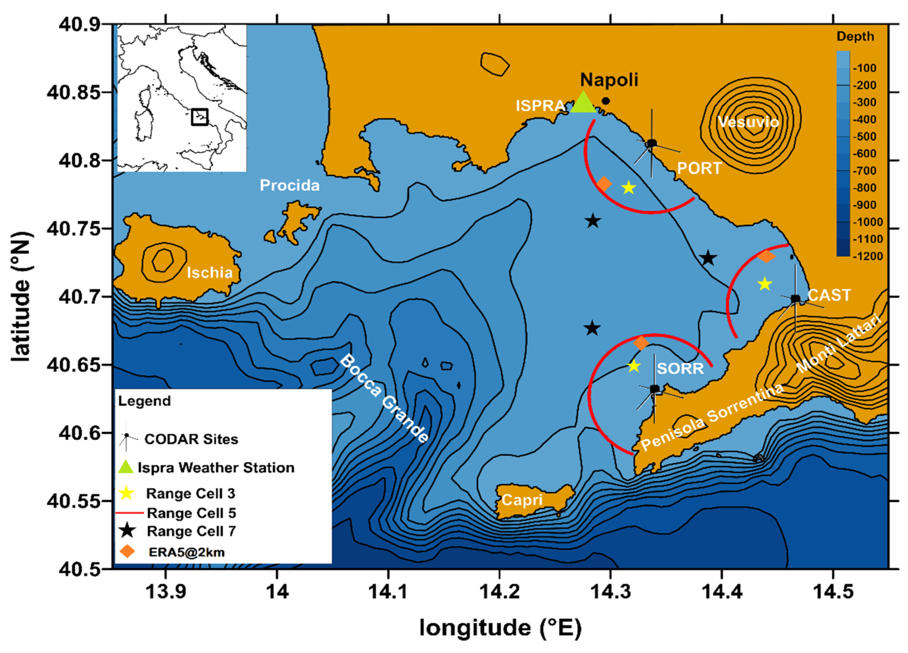
2.1. HFr Network

The GoN HFr network is composed of three sites, located in Portici (PORT), Castellammare di Stabia (CAST) and Massa Lubrense (SORR) (Figure 1). HFr measurements are provided by a CODAR HF system, managed by the Department of Science and Technologies of the Parthenope University, and the wind direction parameter is obtained from the first-order echo, i.e., the same part of the signal used to obtain surface currents [42].
Data are retrieved and averaged along range cells (RCs) centered on each antenna and regularly spaced by 1 km, providing a unique record along each single RC. Owing to this, the directional distribution of the Bragg waves is assumed to be homogeneous over each RC; see [10,43]. Hourly-averaged data from 1 May 2008 to 31 December 2010 and from 1 January 2012 to 31 December 2012 are used.
The performance of HFrs in data acquisition is limited by sources of uncertainty (e.g., environmental noise, distance, interpretation methods), as discussed by [44,45], and can affect the retrievals on RCs differently, as reported in [10]. For the present study, data of all three HFr sites were used. The events retrieved at the PORT site were compared with in situ measurements and model outputs. For the CAST and SORR sites, no comparison with in situ wind directions was possible due to the absence of weather stations in the areas. The results over the year 2011 are not shown due to recurrent failures of the CAST antenna and lower retrieval in these RCs.

2.2. ISPRA Weather Station

To assess the accuracy of the MWM model (see next section) and the HFr, the wind directions were compared with in situ wind observations collected by a weather station managed by Istituto Superiore per la Protezione e la Ricerca Ambientale (ISPRA) and located in the port of Naples (see [29]).
The ISPRA dataset represents, for the analyzed period (2008–2012), the only in situ measurements of the study area. The weather station is representative of local wind data, related to the coastal zone of Naples City affected by topographic steering. This dataset, considering the substantial gradients in the wind direction occurring in coastal regions, is not representative of the conditions of the entire GoN. Consequently, in the comparative analysis, ISPRA data were used only for PORT HF (the closest HF site, located at 13 km distance).
Hourly-averaged data from 1 May 2008 to 31 December 2012 were used in the study.

2.3. Mediterranean Wave Model

The MWM is a model-derived dataset of hourly wave and wind parameters starting from 1 January 1979 and obtained from a chain of the latest-generation models [46,47,48,49]. For more information, see Section 2.3 and Section 2.4 in [28]. The model domain covers the entire Mediterranean Sea, with a spatial resolution of approximately 0.1° (~10 km) in offshore areas, while, in coastal areas or in areas where the depth is less than 100 m, the spatial resolution increases up to approximately 0.03° (~3 km). The wave model is forced by the wind fields obtained from the atmospheric Weather Research and Forecasting Model (WRF). To calibrate and validate the WRF model, some comparisons among different experimental data were used over the Mediterranean (i.e., NOAA stations, ISPRA stations and Puerto del Estado stations). In particular, the Salerno ISPRA station (located in the Gulf of Salerno, south of the GoN) was used in the Tyrrhenian Sea as a reference. The comparison results showed that the model substantially overestimated the measured data. The most severe model overestimation occurrences were recorded when the wind direction was close to the N direction, due to the morphology of the bay and lack of co-located measurements [50].
In the study area, no moored weather buoys were present to use as primary ground truth datasets. To evaluate the model’s performance, a comparison with ERA5@2km in the grid points nearest to the MWM output was developed. Subsequently, a comparison with the Naples ISPRA station provided us with a further, geographically more consistent comparison in the Tyrrhenian Sea area, and it allowed us to compare data between the model and HFr in locations far from the coast, difficult to obtain as experimental measurements.
The comparison between HFr and MWM wind data was carried out along different RCs to assess the retrieval of the wind direction from offshore zones to the coast. HFr wind directions from RC3, RC5 and RC7 (i.e., 3, 5 and 7 km from the antenna, respectively) were analyzed in comparison to those obtained at co-located sites using the MWM model output.

2.4. Statistical Methods

The measurements from three wind data platforms (HFr, ISPRA weather station and MWM model) were analyzed over 44 months, from May 2008 to December 2010 and 2012. During this period, the sea storm events were identified and classified in terms of energy content following [28]. The HFr wind directions retrieved during the storm events were compared with the wind directions obtained from weather station measurements and MWM model outputs.
Wind parameters were seasonally grouped, divided into three-month seasons, as implemented in [28].
Statistical parameters were employed to compare HFr retrievals with the ISPRA and MWM datasets.
As suggested in [29,51], we applied circular statistics parameters for angular variables such as wind direction data to obtain the circular correlation coefficient (ρcc) and mean directional difference (θ) using the Matlab Toolbox CircStat; see [29].
ρ c c = i n sin θ i H F θ H F ¯ sin θ i s i t u θ s i t u ¯ i n sin θ i H F θ H F ¯ 2 n i n sin θ i s i t u θ s i t u ¯ 2 n
ρcc spans the ±1 range, where +1 (−1) indicates perfect correlation (anti-correlation) for two investigated series, while 0 indicates no correlation.
The wind speed comparison between MWM outputs and the ISPRA weather station related to HF PORT RC3 was assessed by means of box plots, correlation coefficients (CCs), root mean square error (RMSE) and the Hanna–Heinold index (HH) proposed in [52].
Box plots, used in descriptive statistics, are a method used to display the distribution of data based on the degree of dispersion and skewness, using five descriptors: the minimum, the maximum, the sample median and the first and third quartiles. The central rectangle spans the first quartile to the third quartile (interquartile range, IQR). A segment inside the rectangle shows the median, and “whiskers” above and below the box show the locations of the first and third quartiles. An outlier is defined as a data point that is located outside the whiskers of the box plot. Box plots that are visually overlapping in terms of the IQR identify statistically similar records.
Finally, the HH index allows us to overcome obstacles that may arise for the negatively biased simulations, i.e., that underestimate the quantities measured (see [53]).

3. Results

To assess the MWM model wind data’s accuracy, the first analysis involved a comparison between the model results and ERA5@2km dataset using the grid point nearest to the model output (RC5) (see Figure 1); subsequently, the comparison between MWM and in situ measurements was carried out.
The MWM model data used in the comparison with the ISPRA weather station were related to the PORT RCs, the HFr site closest to the ISPRA station. The comparison between ERA5@2km and ISPRA did not show significant differences from the comparison with MWM. Subsequently, the results of the comparison among the MWM model, ISPRA and HFr PORT during the storm events was performed. The storm events were analyzed over the entire period of occurrence and during the exceeding threshold of the wind speed.
Comparisons between the HFr sites of CAST and SORR and the MWM model were performed. Results regarding the differences found in the different RCs were obtained for all HFr sites and some of the most relevant events were analyzed in detail.

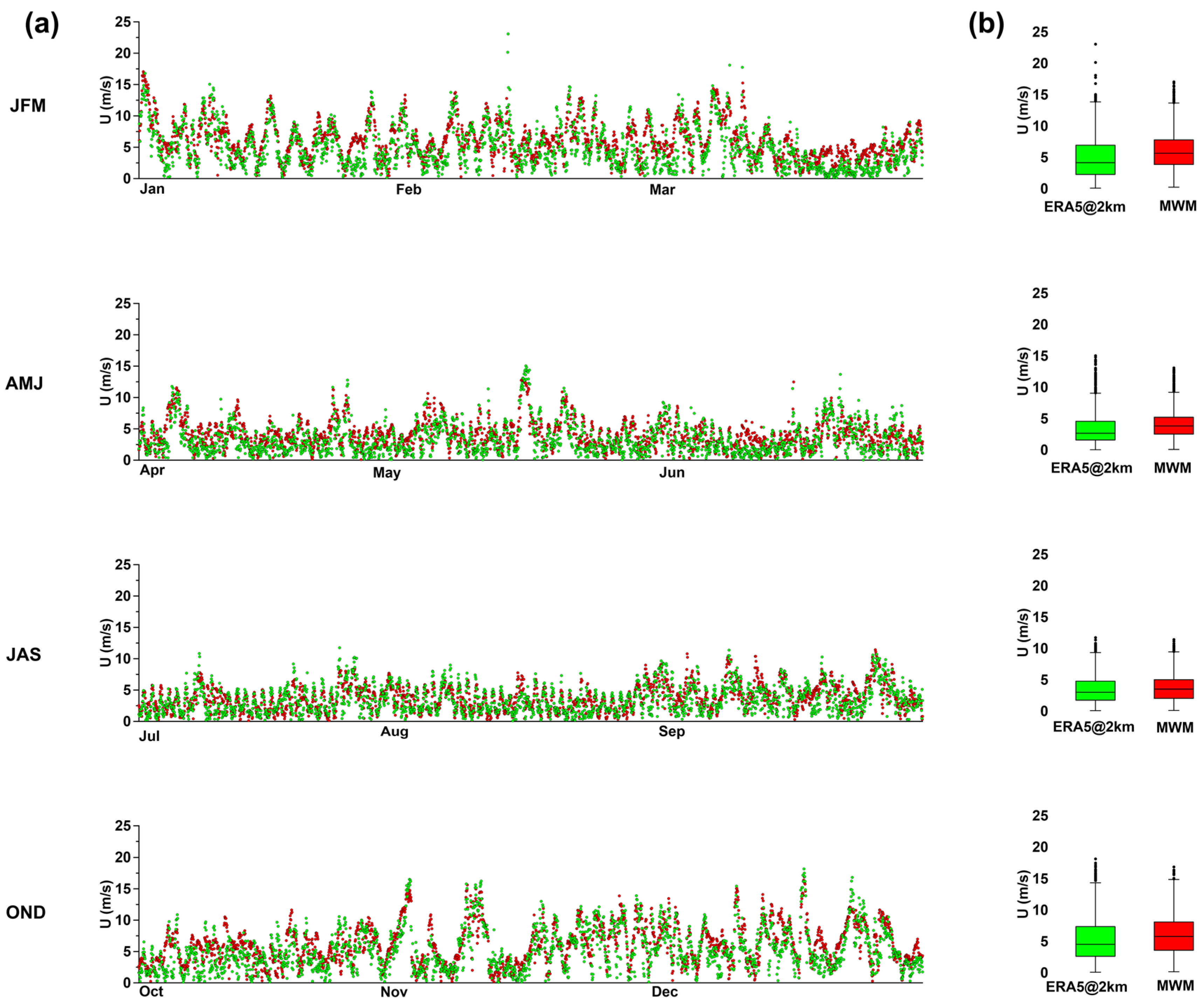
3.1. MWM/ERA5@2km Wind Speed and Wind Direction Comparisons

Figure 2 shows the wind speed time series during the 2010 seasonal trimester at the PORT site (time series in CAST and SORR sites show similar results, figures not presented) and the statistical box plots of both datasets. The comparison shows comparable data between the models during the seasons, as confirmed by the statistical results reported in Table 1 for all the HFr sites in the reference year 2010. The CC values are greater than 0.6 for all trimesters in each site. For each site, the CC values are higher in the autumn and winter seasons, reaching a value of 0.76 in the SORR site; the lower value, with a minimum of 0.6 in the CAST site, was observed during the summer trimester.
Figure 3 shows the wind roses of the MWM and ERA5@2km dataset for the year 2010. The discrepancies between the models are related mainly to the HFr site in the inner part of the GoN; in particular, the CAST site shows two prevalent sectors (NW and SE) in the ERA5@2km dataset, as opposed to the more homogeneous MWM dataset. In the SORR site, the wind directions are comparable over the seasons, likely because the data are related to an external area of the GoN that is less affected by the complex orography. This is confirmed by the statistical analysis shown in Table 2. The mean value over the year 2010 for ρcc is comparable in the SORR site, with a value of 0.63; instead, in PORT and CAST, the comparison does not show significant results. The mean differences over the year show a high value considering the entire dataset, which alternates between periods of agreement (autumn and winter seasons) and long periods of low agreement, in spring and summer, associated with the high atmospheric pressure, mainly in the PORT and CAST sites.

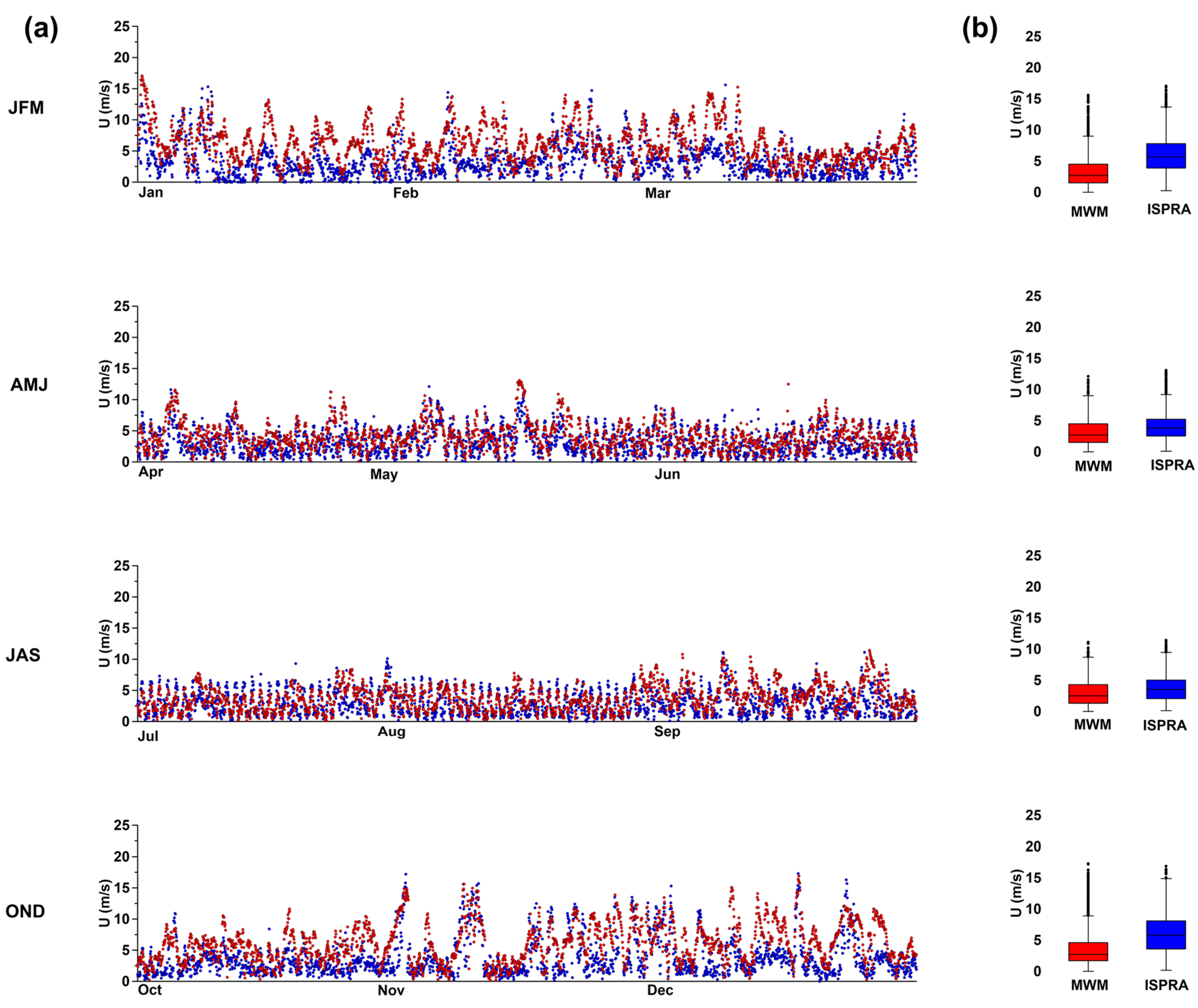
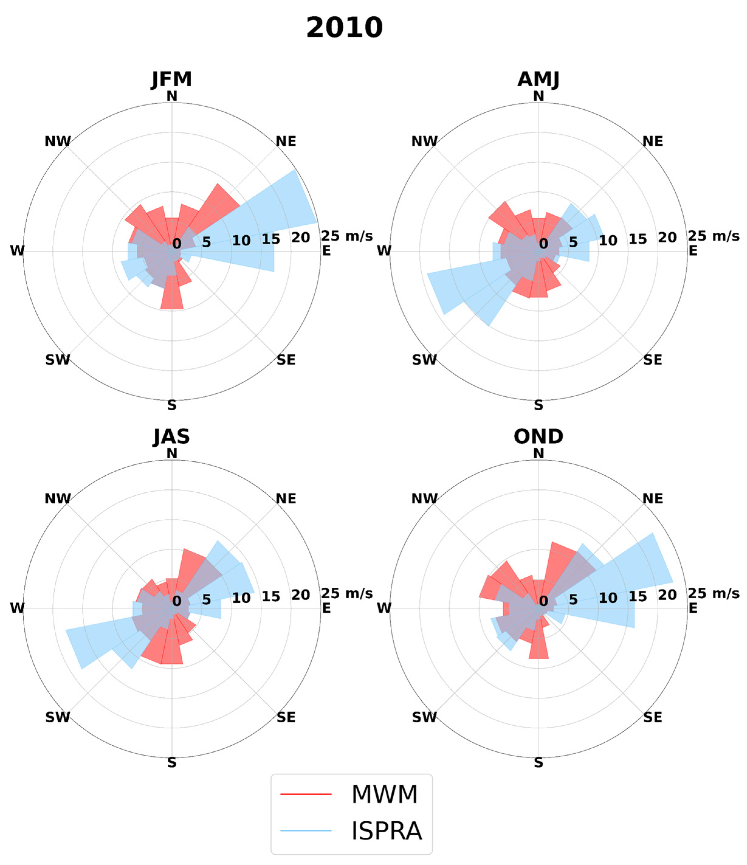
3.2. MWM/ISPRA Wind Speed and Wind Direction Comparisons

The comparison between the ISPRA weather station data and MWM model outputs over RC3, RC5 and RC7 of the PORT site showed discrepancies in the wind speed, mainly in the winter and autumn periods. The time series of wind speed U (m/s) retrieved by ISPRA and simulated by MWM for the year 2010 are presented in Figure 4 (for the complete dataset, see the Supplementary Materials (Figure S1)). Over the winter period, both datasets returned stronger wind events, but the MWM data showed an overestimation with respect to the ISPRA acquisitions. A similar model overestimation was found in previous comparisons in the Tyrrhenian Sea area [50] and can be explained by the strong topographic steering of weather stations in coastal areas (see Section 2.3). All the RCs show a recurrent pattern and values above the 5 m/s threshold are recorded during the winter and autumn seasons, while, during spring and summer, few measurements exceed the threshold. Figure 4b provides the box plot analysis of the wind speed for RC3, RC5 and RC7 related to the PORT site and ISPRA. This analysis confirms the model’s overestimation of the speed parameters in all the RCs; the median values of the ISPRA data are lower than the model outputs for all RCs, but the outlier values are comparable.
The statistical comparisons in Table 3 reveal that RC3 is the most comparable to the ISPRA weather station. RC3 shows CC > 0.5 during all seasons of the reference year 2010 (the complete dataset is shown in the Supplementary Materials (Table S1)). Similar results are found also for RC5; this is justified by the positions of the RCs (closer to the coast) and confirmed by the lower values of CC over the seasons in RC7, far from the coastal area. High values of CC in the summer season are attributable to frequent overestimations in the wind speed when the direction is close to N. The same results are obtained for RMSE, with a minimum value for RC3 in summer and a maximum value for RC7 in the winter season.
The HH index shows again the best results in the model’s performance over RC3, mainly in autumn (0.73), while RC7 in spring shows the highest HH index (0.83).
Figure 5 shows the seasonal wind rose diagrams relative to the year 2010 for the ISPRA and the MWM PORT RC3 data (complete data are shown in the Supplementary Materials (Figure S2–S4)). For ISPRA data, the highest frequencies are obtained for N-NE alternated with S-SW during winter, whereas, during summer and spring, daily alternating SW and NE directions can be observed during all seasons.
MWM shows a wide variety of directions, as shown in Table 4. The statistical parameters of the comparisons between ISPRA and the MWM model appear not to be high throughout the year; ρcc and θ are 0.41 and 58.4°, showing an improvement when using data over the threshold (U > 5 m/s), with values of 0.63 for ρcc and 32.2° for θ. A better result is obtained with respect to the ERA5@2km dataset related to the PORT site, where ρcc is 0.38 and θ is 103.9°.
Again, the MWM outputs show higher intensity than the ISPRA results, likely due to the model’s resolution limitations near the coast (as found in [29] using different model data) and related to the differences in exposure for ISPRA stations with respect to the MWM output point (Figure 1).

3.3. Wind Direction Analysis: MWM, ISPRA and HFr

The comparison between HFr, MWM and in situ data was possible only for the PORT site. The investigations over directions during the sea storm events over the entire period were analyzed, using all the retrievals during the events, and subsequently considering the wind direction data retrieved with wind speed U > 5 m/s. The threshold was identified using the ISPRA wind speed dataset to avoid problems regarding the overestimation of the wind speed by the model results. RC3, RC5 and RC7 of the HF PORT site were used in the comparisons to evaluate the reliability of the HFr retrievals during the storm events. The selection of RCs was based on results obtained in [28,29], where the best agreement was found for RC3 and RC9.
In Table 5, the statistical metrics of the comparison of HFr PORT vs. ISPRA and HFr PORT vs. MWM for the events retrieved in the reference year 2010 are reported considering the wind direction data retrieval with U > 5 m/s (complete dataset is shown in the Supplementary Materials (Table S2)).
The results show agreement among the platforms, with ρcc values > 0.5 in winter and autumn events in both comparisons (HFr vs. ISPRA and HFr vs. MWM). Generally, the HFr data show the best agreement with the ISPRA data, and a mean correlation that is similar for RC3 (0.71) and RC5 (0.71), with a higher correlation for RC7 (0.78). Moreover, the agreement with MWM increases with the distance from the coast, reaching 0.68 for RC7. In spring and summer events, the values of ρcc are lower, while the event in August shows ρcc equal to 0.49 for HFr vs. ISPRA and 0.25 for HFr vs. MWM at RC3, respectively. RMSEs are lower in the comparisons of HFr vs. ISPRA (41.9°) and HFr vs. MWM (45.13°) for RC7.
An analysis of selected events was carried out to demonstrate the differences in considering observations with wind speeds higher or lower than 5 m/s. The first event selected occurred from 4 to 8 December 2008. The upper panel of Figure 6 shows the temporal series of wind speeds (U (m/s)) of the ISPRA weather station and MWM PORT RC3. This event allowed us to investigate the overestimation of the MWM results: when the wind direction was close to the N direction, the model data returned a wind speed > 5 m/s, in conflict with the ISPRA wind speed data, although the wind direction showed agreement. This result was expected from the wind speed analysis (see Section 3.1) and was found in several events in the autumn and winter seasons.
The comparison of the wind directions shows agreement between the platforms when the threshold is exceeded; the maximum speed reached is 16 m/s. The HFr wind direction over the RCs shows a difference mainly in the data retrieved below the threshold. The statistical metrics of the comparison between ISPRA data and MWM data are shown in Table 6. The statistical variables (circular correlation coefficient (ρcc), RMSE and direction difference (θ) were computed over the entire storm period using only the values related to wind speed > 5 m/s. No correlation at RC3 and RC5 and an anticorrelation at RC7 for both comparisons (HF PORT vs. ISPRA and HF PORT vs. MWM) were found. Statistical metrics improved in the observations with U > 5 m/s, showing agreement between HFr PORT vs. ISPRA and HF PORT vs. MWM over RCs with ρcc values > 0.7 for both comparisons.
The event analyzed for HF PORT was observed also in the other two HFr sites. Comparisons between CAST, SORR and the MWM output in regard to RC3, RC5 and RC7 for each site, respectively, were carried out. Unfortunately, in situ data were not available for these two sites. Figure 7 shows the time series of the MWM output and the CAST (upper panel) and SORR sites (lower panel). Lower agreement between HFrs and MWM over RCs is shown, with anticorrelation between the platforms. Results improved at the CAST site when U > 5 m/s, as shown in Table 7. The best agreement was for RC3 at the CAST site, with ρcc of 0.64. The model outputs were similar over RCs in the SORR site, with a maximum value of ρcc equal to 0.7.
Figure 8 shows the event that occurred from 5 May 2010 to 8 May 2010. As shown in the time series, the wind speed exceeded the threshold, reaching a maximum of 12 m/s. Results show better agreement between HFr and ISPRA, with a ρcc value that decreased from the coast to offshore, with higher values at RC3 of 0.49 (0.68) over the entire period (with U > 5 m/s); see Table 8. The comparison with MWM data shows a ρcc value that increases from the coast toward the offshore region, with a ρcc value at RC7 of 0.41 (0.67) over the entire storm period (with U > 5 m/s). RMSE values are lower for the dataset U > 5 m/s for both platforms, while the direction difference is larger at RC7.
Comparisons between CAST, SORR and MWM in regard to RC3, RC5 and RC7 for each site, respectively, were carried out. Figure 9 shows the time series of the wind direction of the MWM at the CAST (upper panel) and SORR (lower panel) sites. Lower agreement between HFrs and MWM over the RCs is shown, and the model outputs are similar over the RCs, mainly in the SORR site. As shown in Table 9, the agreement improves when using data retrieved with U > 5 m/s. The SORR site’s results show an anticorrelation over the RCs with higher values at RC5, from −0.36 over the entire storm period to −0.58 with U > 5 m/s. The CAST site’s results show the best agreement at RC5, with a maximum value of 0.35 for the dataset with U > 5 m/s.

4. Discussion

Wind data at sea are in great demand for various oceanographic applications. Usually, such information can be obtained only from satellite measurements, which are intermittent and may miss important events, or are provided by models. The characteristics of HF radars, with their high spatial and temporal resolutions in coastal areas, make these instruments useful in providing wind data as well as surface currents and wave parameters [7,8].
Investigations of the wind directions retrieved by HF radar systems are rare in the literature, with results showing agreement only under specific wind speed conditions (U > 5 m/s) for both DF and BF systems [17,29].
In [29], a preliminary analysis of the wind direction from a SeaSonde system in the GoN over two months was presented; results were in line with previous studies [54], confirming an increase in the ρcc when the wind speed exceeded the threshold of 5 m/s.
In this work, 44 months of wind direction data from a HFr network were employed, along with MWM model data extracted from grid points corresponding to RC3, RC5 and RC7 of each antenna. During the analyzed period (2008–2010 and 2012), in situ wind measurements of the wind speed and direction were retrieved from the ISPRA weather station. These measurements were strictly linked to the local geomorphology of the GoN, and they were representative of the coastal area of Naples City. ISPRA data were used to validate the numerical data and to compare the HFr PORT sites with local observations and modeled ones.
The first comparative analysis was carried out for wind parameters (speed and direction) between the MWM model and ERA5@2km dataset to assess the quality of the MWM model. The comparison of the wind speed revealed comparable agreement, with a CC around 0.7, mainly in the autumn and winter seasons, in all HFr sites. The wind rose analysis of the PORT and CAST sites, located in the inner part of the GoN, showed a large discrepancy between the datasets due to the low resolutions of models in coastal areas. Instead, better results were obtained for the SORR site, with wind directions comparable over the seasons, due to the position of the grid model output, related to an external area of the GoN that was less affected by the complex morphology of the bay.
These results regarding the model analysis show the observational gaps in coastal regions, which are difficult to address with weather station installations. However, the use of HFr wind data could be a significant aid in improving the model results considering the high spatial and temporal resolutions of such systems [8].
Subsequently, the wind speed and direction obtained from the ISPRA weather station and the MWM model revealed an overestimation on the model data when the wind directions were closer to the N direction. This result confirms a model gap in this wind direction that was previously found during validation and comparison with other weather stations in the Tyrrhenian Sea [47].
Since a comparison with the in situ measurements was possible only for the HFr PORT site, storm events observed for this site were compared with the ISPRA data and MWM outputs, in regard to RC3, RC5 and RC7. The analysis over almost four years of retrieval showed a ρcc value that generally increased with the coastal distance, with a value during the sea storm events of ρcc > 0.7 in the autumn and winter seasons in both comparisons (HF vs. ISPRA and HF vs. MWM), while lower values of ρcc were found in the spring and summer seasons. The ρcc in the HF vs. ISPRA comparison was generally higher in RC3 and RC5, while, in the comparison of HF vs. MWM, the ρcc showed high values in RC7, due to the positions of RC3 and RC5 being closer to the coast and more similar to the ISPRA location, and also ascribable to the coarse resolution of the models in coastal areas [28].
HFr CAST and SORR observations could only be compared with the MWM model outputs. Results showed low agreement between the platforms, with the CAST site returning low ρcc values over the years, with a few cases of ρcc > 0.5 at RC5 during the storm events. On the other hand, the SORR site in the comparison with MWM over the RCs showed an anticorrelation that increased during the storm period, with ρcc > −0.7 in the autumn and winter seasons. The discrepancies in the comparison of CAST and SORR can be related to the lack of measurement of the wind speed. In fact, the reference used to identify the threshold (U > 5 m/s) was the ISPRA wind speed data, but, considering the geomorphology and the distance between the sites, the local response may be different. This confirms the requirement of in situ measurements co-located with HFr for data validation and to support investigations of inversion methods and possible parameters leading to measurement failure.
The HFr spectrum contains information about the local wind (wind sea) and swell (generated by winds away from the area), and the relationship between the local wind sea and wind speed depends on the fetch and duration. Recently, for WERA systems, an alternative approach was developed using machine learning to develop a physical model to extract the wind speed from the radar signal [16]. This method achieved acceptable accuracy, but further investigations are needed.

5. Conclusions

A comparison between in situ measurements and data from the MWM model has been employed using 44 months of retrievals, from May 2008 to December 2010 and 2012, by a network of three SeaSonde HFr systems in the GoN.
The MWM model data analysis highlights inconsistencies between the wind direction measurements compared to what was observed for the speed. In fact, comparisons between MWM, ERA5@2km and ISPRA show that further improvements are needed that better take into account the local conditions that may occur near the coast.
The results confirm that HFr retrievals are more comparable with other measurements (in situ or model data) when the wind speed exceeds 5 m/s, i.e., in the study area during sea storm events. The investigations in the GoN reveal the strong dependence of the wind data quality on the seasonality of the study area, characterized by short periods in which the conditions (speed > 5 m/s) are verified. These limitations reduce the potentiality of these instruments. To make HFr wind retrievals usable, it is necessary to investigate inversion methods and perform further investigations in other areas where SeaSonde systems are operational, to obtain surface current and wave data with dynamics that are different from those of the GoN. Once the results are validated, the HFr wind data could be used to improve the model results in coastal areas, i.e., through data assimilation.

Supplementary Materials

The following supporting information can be downloaded at: https://0-www-mdpi-com.brum.beds.ac.uk/article/10.3390/rs15122991/s1, Figure S1: (a). Temporal series of wind speed from May 2008 to December 2012 of ISPRA (blue) and DHI model at RC3, RC5, RC7 of PORT site (red); the black line represents the wind speed threshold (5 m/s). (b). Box plots of the dataset; the outliers are identified by red crosses. Table S1: Statistical metrics (correlation coefficient (CC), root mean square error (RMSE) and Hanna–Heinold index (HH)) of wind speed between the MWM model and ISPRA, seasonal comparison (2008-2009-2012). Year 2010 is shown in the text, see Table 3. Figure S2: The left panel shows the seasonal wind direction for the year 2008 at the ISPRA weather station. Right panel shows the seasonal wind direction for the year 2008 in the MWM model at PORT-RC3. Figure S3: The left panel shows the seasonal wind direction for the year 2009 at the ISPRA weather station. Right panel shows the seasonal wind direction for the year 2009 in the MWM model at PORT-RC3. Figure S4: The left panel shows the seasonal wind direction for the year 2012 at the ISPRA weather station. Right panel shows the seasonal wind direction for the year 2012 in the MWM model at PORT-RC3. Table S2: Statistical metrics of comparisons among HF PORT site, ISPRA weather station and MWM model wind directions with wind speed U > 5 m/s at RC5 for the years 2008, 2009 and 2012. Year 2010 is shown in the text, see Table 5.

Author Contributions

Methodology: S.S., D.C. and M.U.; software: S.S. and A.A.B.; validation: S.S., A.A.B., D.C. and M.U.; model data: F.K., L.A.C. and A.P.; data curation: A.A.B., F.K. and S.S.; writing—review and editing: S.S., A.A.B., D.C., M.U. and E.Z.; project administration: D.C. All authors have read and agreed to the published version of the manuscript.

Funding

S.S. was supported by Stazione Zoologica Anton Dohrn PON PRIMA (project CIR01_00029); E.Z. was partly supported by the 2017 PRIN project EMME (Exploring the fate of Mediterranean microplastic: from distribution pathways to biological effects), funded by the Italian Ministry for Research (grant agreement no. 2017WERYZP).

Data Availability Statement

The data presented in this study are openly available at the links provided in the text.

Acknowledgments

The Department of Science and Technology of the Parthenope University of Naples operates the HF radar system on behalf of the AMRA consortium (formerly CRdC AMRA), a regional competence center for the analysis and monitoring of environmental risks. Our remote radar sites are hosted by the ENEA Centre of Portici, the Villa Angelina Village of High Education and Professional Training and La Villanella resort in Massa Lubrense, and the Fincantieri shipyard in Castellammare di Stabia, whose hospitality is gratefully acknowledged. Mention of trade names or commercial products does not constitute endorsement or recommendation. We thank Roberta Di Lemma and Giovanni Esposito for the useful discussion on data analysis. Technical support from Giovanni Zambardino was invaluable for the proper functioning of the HF radar system.

Conflicts of Interest

The authors declare no conflict of interest.

References

  1. Roarty, H.; Cook, T.; Hazard, L.; George, D.; Harlan, J.; Cosoli, S.; Wyatt, L.; Alvarez Fanjul, E.; Terrill, E.; Otero, M.; et al. The Global High Frequency Radar Network. Front. Mar. Sci. 2019, 6, 164. [Google Scholar] [CrossRef]
  2. Huang, W.; Gill, E.W. (Eds.) Ocean Remote Sensing Technologies—High-Frequency, Marine and GNSS-Based Radar; SciTech Publishing: Luxembourg, 2021. [Google Scholar]
  3. Tseng, Y.H.; Lu, C.Y.; Zheng, Q.; Ho, C.R. Characteristic analysis of sea surface currents around Taiwan Island from CODAR observations. Remote Sens. 2021, 13, 3025. [Google Scholar] [CrossRef]
  4. Rubio, A.; Mader, J.; Corgnati, L.; Mantovani, C.; Griffa, A.; Novellino, A.; Quentin, C.; Wyatt, L.; Schulz-Stellenfleth, J.; Horstmann, J.; et al. HF radar activity in European coastal seas: Next steps toward a pan-European HF radar network. Front. Mar. Sci. 2017, 4, 8. [Google Scholar] [CrossRef] [Green Version]
  5. Gurgel, K.-W.; Antonischki, G.; Essen, H.-H.; Schlick, T. Wellen radar WERA: A new ground-wave HF radar for ocean remote sensing. Coast. Eng. 1999, 37, 219–234. [Google Scholar] [CrossRef]
  6. Barrick, D.E. Extraction of wave parameters from measured HF radar sea-echo Doppler spectra. Radio Sci. 1977, 12, 415–424. [Google Scholar] [CrossRef]
  7. Lorente, P.; Aguiar, E.; Bendoni, M.; Berta, M.; Brandini, C.; Cáceres-Euse, A.; Capodici, F.; Cianelli, D.; Ciraolo, G.; Corgnati, L.; et al. Coastal high-frequency radars in the Mediterranean—Part 1: Status of operations and a framework for future development. Ocean Sci. 2022, 18, 761–795. [Google Scholar] [CrossRef]
  8. Reyes, E.; Aguiar, E.; Bendoni, M.; Berta, M.; Brandini, C.; Cáceres-Euse, A.; Capodici, F.; Cardin, V.; Cianelli, D.; Ciraolo, G.; et al. Coastal high-frequency radars in the Medi-terranean—Part 2: Applications in support of science priorities and societal needs. Ocean Sci. 2022, 18, 797–837. [Google Scholar] [CrossRef]
  9. Wyatt, L. Ocean wave measurement. In Ocean Remote Sensing Technologies—High-Frequency, Marine and GNSS-Based Radar; Huang, W., Gill, E.W., Eds.; SciTech Publishing: Raleigh, NC, USA, 2021; pp. 145–178. [Google Scholar]
  10. Saviano, S.; Kalampokis, A.; Zambianchi, E.; Uttieri, M. A year-long assessment of wave measurements retrieved from an HF radar network in the Gulf of Naples (Tyrrhenian Sea, Western Mediterranean Sea). J. Oper. Oceanogr. 2019, 12, 1–15. [Google Scholar] [CrossRef]
  11. Saviano, S.; De Leo, F.; Besio, G.; Zambianchi, E.; Uttieri, M. HF Radar Measurements of Surface Waves in the Gulf of Naples (Southeastern Tyrrhenian Sea): Comparison With Hindcast Results at Different Scales. Front. Mar. Sci. 2020, 7, 492. [Google Scholar] [CrossRef]
  12. Basañez, A.; Lorente, P.; Montero, P.; Álvarez-Fanjul, E.; Pérez-Muñuzuri, V. Quality Assessment and practical interpretation of the wave parameters estimated by HF Radars in NW Spain. Remote Sens. 2020, 12, 598. [Google Scholar] [CrossRef] [Green Version]
  13. Bué, I.; Semedo, Á.; Catalão, J. Evaluation of HF Radar Wave Measurements in Iberian Peninsula by Comparison with Satellite Altimetry and in Situ Wave Buoy Observations. Remote Sens. 2020, 12, 3623. [Google Scholar] [CrossRef]
  14. Lorente, P.; Lin-Ye, J.; García-León, M.; Reyes, E.; Fernandes, M.; Sotillo, M.G.; Espino, M.; Ruiz, M.I.; Gracia, V.; Perez, S.; et al. On the Performance of High Frequency Radar in the Western Mediterranean During the Record-Breaking Storm Gloria. Front. Mar. Sci. 2021, 8, 205. [Google Scholar] [CrossRef]
  15. Ludeno, G.; Uttieri, M. Editorial for Special Issue “Radar Technology for Coastal Areas and Open Sea Monitoring”. J. Mar. Sci. Eng. 2020, 8, 560. [Google Scholar] [CrossRef]
  16. Wyatt, L.R. Progress towards an HF Radar Wind Speed Measurement Method Using Machine Learning. Remote Sens. 2022, 14, 2098. [Google Scholar] [CrossRef]
  17. Wyatt, L.R.; Green, J.J. Swell and wind-sea partitioning of HF radar directional spectra. J. Oper. Oceanogr. 2022. [Google Scholar] [CrossRef]
  18. Lopez, G.; Conley, D.C. Comparison of HF Radar Fields of Directional Wave Spectra Against In Situ Measurements at Multiple Locations. J. Mar. Sci. Eng. 2019, 7, 271. [Google Scholar] [CrossRef] [Green Version]
  19. Wyatt, L.R. A comparison of scatterometer and HF radar wind direction measurements. J. Oper. Oceanogr. 2018, 11, 54–63. [Google Scholar] [CrossRef]
  20. Falco, P.; Buonocore, B.; Cianelli, D.; De Luca, L.; Giordano, A.; Iermano, I.; Kalampokis, A.; Saviano, S.; Uttieri, M.; Zambardino, G. Dynamics and sea state in the Gulf of Naples: Potential use of high-frequency radar data in an operational oceanographic context. J. Oper. Oceanogr. 2016, 9, 33–45. [Google Scholar] [CrossRef] [Green Version]
  21. Mali, M.; Di Leo, A.; Giandomenico, S.; Spada, L.; Cardellicchio, N.; Calò, M.; Fedele, A.; Ferraro, L.; Milia, A.; Renzi, M.; et al. Multivariate tools to investigate the spatial contaminant distribution in a highly anthropized area (Gulf of Naples, Italy). Environ. Sci. Pollut. Res. 2022, 29, 62281–62298. [Google Scholar] [CrossRef]
  22. Del Gaizo, G.; Russo, L.; Abagnale, M.; Buondonno, A.; Furia, M.; Saviano, S.; Vargiu, M.; Conversano, F.; Margiotta, F.; Saggiomo, M.; et al. An autumn biodiversity survey on heterotrophic and mixotrophic protists along a coast-to-offshore transect in the Gulf of Naples (Italy). Adv. Oceanogr. Limnol. 2021, 12. [Google Scholar] [CrossRef]
  23. Uttieri, M.; Cianelli, D.; Buongiorno Nardelli, B.; Buonocore, B.; Falco, P.; Colella, S.; Zambianchi, E. Multiplatform observation of the surface circulation in the Gulf of Naples (Southern Tyrrhenian Sea). Ocean Dyn. 2011, 61, 779–796. [Google Scholar] [CrossRef]
  24. Cianelli, D.; D’Alelio, D.; Uttieri, M.; Sarno, D.; Zingone, A.; Zambianchi, E.; Ribera d’Alcalà, M. Disentangling physical and biological drivers of phytoplankton dynamics in a coastal system. Sci. Rep. 2017, 7, 15868. [Google Scholar] [CrossRef] [PubMed] [Green Version]
  25. Kokoszka, F.; Saviano, S.; Botte, V.; Iudicone, D.; Zambianchi, E.; Cianelli, D. Gulf of Naples Advanced Model (GNAM): A Multiannual Comparison with Coastal HF Radar Data and Hydrological Measurements in a Coastal Tyrrhenian Basin. J. Mar. Sci. Eng. 2022, 10, 1044. [Google Scholar] [CrossRef]
  26. Iermano, I.; Moore, A.M.; Zambianchi, E. Impacts of a 4-dimensional variational data assimilation in a coastal ocean model of southern Tyrrhenian Sea. J. Mar. Syst. 2016, 154, 157–171. [Google Scholar] [CrossRef]
  27. Saviano, S.; Cianelli, D.; Zambianchi, E.; Conversano, F.; Uttieri, M. An Integrated Reconstruction of the Multiannual Wave Pattern in the Gulf of Naples (South-Eastern Tyrrhenian Sea, Western Mediterranean Sea). J. Mar. Sci. Eng. 2020, 8, 372. [Google Scholar] [CrossRef]
  28. Saviano, S.; Biancardi, A.A.; Uttieri, M.; Zambianchi, E.; Cusati, L.A.; Pedroncini, A.; Contento, G.; Cianelli, D. Sea Storm Analysis: Evaluation of Multiannual Wave Parameters Retrieved from HF Radar and Wave Model. Remote Sens. 2022, 14, 1696. [Google Scholar] [CrossRef]
  29. Saviano, S.; Esposito, G.; Di Lemma, R.; de Ruggiero, P.; Zambianchi, E.; Pierini, S.; Falco, P.; Buonocore, B.; Cianelli, D.; Uttieri, M. Wind Direction Data from a Coastal HF Radar System in the Gulf of Naples (Central Mediterranean Sea). Remote Sens. 2021, 13, 1333. [Google Scholar] [CrossRef]
  30. Menna, M.; Mercatini, A.; Uttieri, M.; Buonocore, B.; Zambianchi, E. Wintertime transport processes in the Gulf of Naples investigated by HF radar measurements of surface currents. II Nuovo Cim. C 2007, 30, 605–622. [Google Scholar]
  31. Prati, M.V.; Costagliola, M.A.; Quaranta, F.; Murena, F. Assessment of ambient air quality in the port of Naples. J. Air Waste Manag. Assoc. 2015, 65, 970–979. [Google Scholar] [CrossRef] [Green Version]
  32. Montuori, A.; de Ruggiero, P.; Migliaccio, M.; Pierini, S.; Spezie, G. X-band COSMO- SkyMedc wind field retrieval, with application to coastal circulation modeling. Ocean Sci. 2013, 9, 121–132. [Google Scholar] [CrossRef] [Green Version]
  33. de Ruggiero, P. A high-resolution ocean circulation model of the Gulf of Naples and adjacent areas. II Nuovo Cim. C 2013, 36, 143–150. [Google Scholar]
  34. Hatzaki, M.; Flocas, H.A.; Simmonds, I.; Kouroutzoglou, J.; Keay, K.; Rudeva, I. Seasonal aspects of an objective climatology of anticyclones affecting the Mediterranean. J. Clim. 2014, 27, 9272–9289. [Google Scholar] [CrossRef]
  35. de Ruggiero, P.; Esposito, G.; Napolitano, E.; Iacono, R.; Pierini, S.; Zambianchi, E. Modelling the marine circulation of the Campania coastal system (Tyrrhenian Sea) for the year 2016: Analysis of the dynamics. J. Mar. Syst. 2020, 210, 103388. [Google Scholar] [CrossRef]
  36. Castagno, P.; de Ruggiero, P.; Pierini, S.; Zambianchi, E.; De Alteris, A.; De Stefano, M.; Budillon, G. Hydrographic and dynamical characterisation of the Bagnoli-Coroglio Bay (Gulf of Naples, Tyrrhenian Sea). Chem. Ecol. 2020, 36, 598–618. [Google Scholar] [CrossRef]
  37. De Maio, A.; Moretti, M.; Sansone, E.; Spezie, G.; Vultaggio, M. Outline of marine currents in the Bay of Naples and some considerations on pollutant transport. II Nuovo Cim. C 1985, 8, 955–969. [Google Scholar] [CrossRef]
  38. Cianelli, D.; Uttieri, M.; Buonocore, B.; Falco, P.; Zambardino, G.; Zambianchi, E. Dynamics of a Very Special Mediterranean Coastal Area: The Gulf of Naples, in Mediterranean Ecosystems: Dynamics, Management and Conservation; Williams, G., Ed.; Nova Science Publishers: New York, NY, USA, 2012; pp. 129–150. [Google Scholar]
  39. Landberg, L.; Giebel, G.; Nielsen, H.A.; Nielsen, T.; Madsen, H. Short-term prediction—An overview. Wind Energy 2003, 6, 273–280. [Google Scholar] [CrossRef]
  40. Hersbach, H.; Bell, B.; Berrisford, P.; Hirahara, S.; Horányi, A.; Muñoz-Sabater, J.; Nicolas, J.; Peubey, C.; Radu, R.; Schepers, D.; et al. The ERA5 global reanalysis. Q. J. R. Meteorol. Soc. 2020, 146, 1999–2049. [Google Scholar] [CrossRef]
  41. Reder, A.; Raffa, M.; Padulano, R.; Rianna, G.; Mercogliano, P. Characterizing extreme values of precipitation at very high resolution: An experiment over twenty European cities. Weather. Clim. Extrem. 2022, 35, 100407. [Google Scholar] [CrossRef]
  42. Lipa, B.; Daugharty, M.; Fernandes, M.; Barrick, D.; Alonso-Martinera, A.; Roarty, H.; Dicopoulos, J.; Whelan, C. Developments in compact HF-radar ocean wave measurement. In Advances in Sensors: Reviews; Yurish, S.Y., Ed.; IFSA Publishing: Barcelona, Spain, 2018; Volume 5, pp. 469–495. [Google Scholar]
  43. Lipa, B.; Barrick, D.; Alonso-Martirena, A.; Fernandes, M.; Ferrer, M.I.; Nyden, B. Brahan project high frequency radar ocean measurements: Currents, winds, waves and their interactions. Remote Sens. 2014, 6, 12094–12117. [Google Scholar] [CrossRef] [Green Version]
  44. Laws, K.; Paduan, J.D.; Vesecky, J. Estimation and assessment of errors related to antenna pattern distortion in CODAR SeaSonde high-frequency radar ocean current measurements. J. Atmos. Ocean. Technol. 2010, 27, 1029–1043. [Google Scholar] [CrossRef] [Green Version]
  45. Lipa, B.; Nyden, B.; Barrick, D.; Kohut, J. HF radar sea-echo from shallow water. Sensors 2008, 8, 4611–4635. [Google Scholar] [CrossRef] [PubMed]
  46. Saha, S.; Moorthi, S.; Pan, H.-L.; Wu, X.; Wang, J.; Nadiga, S.; Tripp, P.; Kistler, R.; Woollen, J.; Behringer, D.; et al. NCEP Climate Forecast System Reanalysis (CFSR) Selected Hourly Time-Series Products, January 1979 to December 2010. Bull. Am. Meteorol. Soc. 2010, 91, 1015–1058. [Google Scholar] [CrossRef] [Green Version]
  47. Skamarock, W.C.; Klemp, J.B. A time-split nonhydrostatic atmospheric model for weather research and forecasting applications. J. Comput. Phys. 2008, 227, 3465–3485. [Google Scholar] [CrossRef]
  48. Michalakes, J.; Chen, S.; Dudhia, J.; Hart, L.; Klemp, J.; Middlecoff, J.; Skamarock, W. Development of a Next Generation RegionalWeather Research and Forecast Model. Developments in Teracomputing. In Developments in Teracomputing, Proceedings of the 9th ECMWF Workshop on the Use of High Performance Computing in Meteorology; Reading, UK, 13–17 November 2000; Zwieflhofer, W., Kreitz, N., Eds.; World Scientific: Singapore, 2001; pp. 269–276. [Google Scholar]
  49. Sorensen, O.R.; Kofoed-Hansen, H.; Rugbjerg, M.; Sorensen, L.S. A Third Generation Spectral Wave Model Using an Unstructured Finite Volume Technique. In Proceedings of the 29th International Conference of Coastal Engineering, Lisbon, Portugal, 19–24 September 2004. [Google Scholar]
  50. Technical Report SEAPOL Project. Sistema modellistico ad Elevata risoluzione per l’Analisi storica e la Previsione del moto Ondoso nel mar Ligure POR-FESR (2007–2010)—Asse 1 Innovazione e Competitività, Bando DLTM, Azione 1.2.2 “Ricerca industriale e sviluppo sperimentale a favore delle imprese del Distretto Ligure per le Tecnologie Marine (DLTM), Pos. n° 47”. DHI Italia.
  51. Ranalli, M.; Lagona, F.; Picone, M.; Zambianchi, E. Segmentation of sea current fields by cylindrical hidden Markov models: A composite likelihood approach. J. R. Stat. Soc. Ser. C 2018, 67, 575–598. [Google Scholar] [CrossRef]
  52. Hanna, S.; Heinold, D. Development and Application of a Simple Method for Evaluating Air Quality; Technical Report; American Petroleum Institute, Health and Environmental Affairs Department, Pennsylvania State University: State College, PA, USA, 1985. [Google Scholar]
  53. Mentaschi, L.; Besio, G.; Cassola, F.; Mazzino, A. Problems in RMSE-based wave model validations. Ocean Modell. 2013, 72, 53–58. [Google Scholar] [CrossRef]
  54. Shen, W.; Gurgel, K.-W. Wind direction inversion from narrow-beam HF Radar backscatter signals in low and high wind conditions at different radar frequencies. Remote Sens. 2018, 10, 1480. [Google Scholar] [CrossRef] [Green Version]
Figure 1. Map of the Gulf of Naples (Central Tyrrhenian Sea, Western Mediterranean Sea) with the locations of the three HF radar sites (antennas) and of the ISPRA weather station (green triangle). The red semi-circles represent Range Cell 5 (RC5); yellow and black stars represent Range Cell 3 (RC3) and Range Cell 7 (RC7), respectively (see text). MWM model data are co-located with RC3, RC5 and RC7 for each site. Orange diamonds indicate the ERA5@2km grid points. The bathymetric contours are spaced every 100 m; the orographic ones are spaced every 300 m.
Remotesensing 15 02991 g001
Figure 2. (a) shows the temporal series of wind speed for the seasonal trimesters of 2010 for the MWM model (red) and ERA5@2km dataset (green) at RC5 in the PORT site; (b) shows the statistical box plots of the dataset.
Remotesensing 15 02991 g002
Figure 3. Wind rose comparison of MWM (red) and ERA5@2km (green) for each site for the year 2010.
Remotesensing 15 02991 g003
Figure 4. (a) shows a seasonal temporal series of wind speed for 2010 for ISPRA (blue) and the MWM model at RC5 in PORT site (red); (b) reports the box plots of the dataset, where the outliers are identified by crosses.
Remotesensing 15 02991 g004
Figure 5. The panels show the seasonal wind roses for the year 2010 for the ISPRA weather station (light blue) and MWM model (red) at PORT for RC3.
Remotesensing 15 02991 g005
Figure 6. Event that occurred from 4 December 2008 to 8 December 2008. First panel shows wind speed (U (m/s)) from ISPRA (blue) and MWM PORT RC3 (red), with dotted line representing the threshold of 5 m/s. Lower panels show the wind direction (Dir(°)) of HFr PORT RC3, RC5, RC7 with ISPRA and MWM datasets, respectively.
Remotesensing 15 02991 g006
Figure 7. Event that occurred from 4 December 2008 to 8 December 2008. The upper panels show the wind direction (Dir(°)) at RC3, RC5, RC7 for HFr CAST site and MWM output over RCs. The lower panels show the wind direction (Dir(°)) at RC3, RC5, RC7 for the HFr SORR site and the MWM in regard to the three RCs, respectively.
Remotesensing 15 02991 g007
Figure 8. Event that occurred from 5 May 2010 to 8 May 2010. First panel shows wind speed (U (m/s)) from ISPRA (blue) and MWM PORT RC3 (red), with dotted line representing the threshold of 5 m/s. Lower panels show the wind direction (Dir(°)) of HFr PORT RC3, RC5, RC7 with ISPRA and MWM datasets, respectively.
Remotesensing 15 02991 g008
Figure 9. Event that occurred from 5 May 2010 to 8 May 2010. The upper panels show the wind direction (Dir(°)) at RC3, RC5, RC7 for HFr CAST site and MWM output over RCs. The lower panels show the wind direction (Dir(°)) at RC3, RC5, RC7 for HFr SORR site and MWM output over RCs, respectively.
Remotesensing 15 02991 g009
Table 1. Statistical metrics (correlation coefficient (CC), root mean square error (RMSE) and Hanna–Heinold index (HH)) of wind speed between the MWM model and ERA5@2km, seasonal comparison (2010) at RC5 of PORT, CAST and SORR sites.
2010MWM vs. ERA5@2km
TrimesterPORTCASTSORR
CCRMSEHHCCRMSEHHCCRMSEHH
JFM0.712.680.440.672.880.440.732.830.38
AMJ0.642.140.510.622.260.50.672.430.49
JAS0.631.830.460.61.950.460.632.150.48
OND0.712.60.410.662.980.450.762.650.35
Table 2. Statistical parameters (ρcc, RMSE and θ) in the comparisons between the MWM model and ERA5@2km wind direction in the year 2010 at RC5 for PORT, CAST and SORR sites.
MWM vs. ERA5@2km
2010PORTCASTSORR
ρccRMSEθρccRMSEθρccRMSEθ
0.3842.1583.90.2281.997.30.6367.0567.9
Table 3. Statistical metrics (correlation coefficient (CC), root mean square error (RMSE) and Hanna–Heinold index (HH)) of wind speed between the MWM model and ISPRA, seasonal comparison (2010).
ISPRA vs. MWM
Wind Speed
RC3RC5RC7
2010 TrimesterCCRMSE (m/s)HHCCRMSE (m/s)HHCCRMSE (m/s)HH
Winter (JFM)0.513.650.760.493.930.80.474.290.86
Spring (AMJ)0.52.210.580.492.350.60.472.540.64
Summer (JAS)0.472.120.610.442.260.640.42.460.68
Autumn (OND)0.623.30.630.613.550.670.593.870.71
Table 4. Statistical parameters (ρcc, RMSE and θ) of the comparisons between the MWM model and ISPRA wind direction in the year 2010 at the PORT site.
MWM vs. ISPRA
PORT
ρccRMSEθ
20100.4141.658
2010 (U > 5 m/s)0.6733.332
Table 5. Statistical metrics of the comparisons among the HF PORT site, ISPRA weather station and MWM model wind directions in 2010 for wind speed U > 5 m/s.
2010RC3
HF vs. ISPRAHF vs. MWM
Eventρccθ (°)RMSE (°)ρccθ (°)RMSE (°)
Jan_1_30.6436.347.30.5221.336.9
Feb_5_70.87−7.94310.93−10.439.8
Apr_1_60.8216.158.280.74−3.1542.8
Apr_19_210.7820.943.90.96−1035.7
May_5_80.68−10.954.50.61−28.859.9
May_13_180.6140.757.40.3623.935.4
Aug_28_300.49−1641.80.25−47.756.8
Sep_25_290.661648.40.395.437.3
Nov_18_230.69−2643.70.64−44.156.8
Dic_1_50.84−11.148.80.77−26.948.5
Dic_23_260.69−32.648.20.56−46.656.2
Mean0.712.3348.70.61−15.246.01
RC5
Jan_1_30.6923.6543.230.579.135.14
Feb_5_70.91−3.8335.770.89−6.6637.77
Apr_1_60.824.5358.810.724.2439.27
Apr_19_210.797.5651.270.94−22.748.73
May_5_80.55−28.454.580.54−4662.23
May_13_180.5634.3957.090.46−46.528.35
Aug_28_300.58−6.5735.540.3314.351.79
Sep_25_290.5926.146.880.3516.3728.68
Nov_18_230.71−29.541.650.67−47.255.32
Dic_1_50.79−19.740.610.65−37.144.37
Dic_23_260.86−31.544.740.8−42.752.58
Mean0.71−0.3646.40.63−18.644.02
RC7
Jan_1_30.66−21.646.50.73−37.851.7
Feb_5_70.88−17.334.20.9−22.239.8
Apr_1_60.82−2.5548.530.7−20.532.6
Apr_19_210.811.8546.830.94−22.845.07
May_5_80.63−43.752.220.67−62.467.7
May_13_180.7−17.349.50.27−41.431.2
Aug_28_300.81−16.639.10.56−38.449.3
Sep_25_290.89−5.4538.170.44−19.428.3
Nov_18_230.85−31.536.530.76−51.956.2
Dic_1_50.76−29.334.550.69−48.747.9
Dic_23_260.81−28.735.050.82−41.946.65
Mean0.78−18.441.90.68−37.145.13
Table 6. Statistical parameters (ρcc, RMSE and θ) of the comparisons between HFr PORT, ISPRA weather station and MWM model during the event on 4–8 December 2008.
Comparison
Event 4–8 December 2008
Observation Number (h)ρccRMSE (°)θ (°)Observation Number
(U > 5 m/s)
ρcc
(U > 5 m/s)
RMSE (°)
(U > 5 m/s)
θ (°)
(U > 5 m/s)
RC3
HFr-ISPRA109−0.0448.8571280.7450.8847
HFr-MWM1090.1347.9674.01280.8461.956.47
RC5
HFr-ISPRA109−0.1839.6575280.6949.747
HFr-MWM109053.9971.23280.7765.462.43
RC7
HFr-ISPRA109−0.5934.8562280.7338.9936
HFr-MWM109−0.5255.0470.17280.8458.9157.99
Table 7. Statistical parameters (ρcc, RMSE and θ) of the comparisons between HFr (CAST and SORR) and MWM model related to the event (4–8 December 2008).
Comparison
Event 4–8
December 2008
Observation Number (h)ρccRMSE (°)θ (°)Observation Number
(U > 5 m/s)
ρcc
(U > 5 m/s)
RMSE (°)
(U > 5 m/s)
θ (°)
(U > 5 m/s)
RC3
CAST-MWM109−0.6549.9877.52280.6471.1473.17
SORR-MWM1090.623.8745.8228−0.3823.4519.68
RC5
CAST-MWM109−0.5947.3759.11280.3060.561.89
SORR-MWM109−0.932.0341.9828−0.6724.718.99
RC7
CAST-MWM1090.5845.5261.32280.0552.3717.37
SORR-MWM109−0.8331.8246.2928−0.728.126.12
Table 8. Statistical parameters (ρcc, RMSE and θ) of the comparisons between HFr PORT, ISPRA weather station and MWM model related to event (5–8 May 2010).
Comparison
Event 5–8 May 2010
Observation Number (h)ρccRMSE (°)θ (°)Observation Number
(U > 5 m/s)
ρcc
(U > 5 m/s)
RMSE (°)
(U > 5 m/s)
θ (°)
(U > 5 m/s)
RC3
HFr-ISPRA960.4955.761390.6854.550
HFr-MWM960.3163.569.04390.6159.957.93
RC5
HFr-ISPRA960.4453.460390.5554.649
HFr-MWM960.3363.965.9390.5462.258.48
RC7
HFr-ISPRA960.3952.761390.6352.247
HFr-MWM960.4167.570.98390.6767.763.65
Table 9. Statistical parameters (ρcc, RMSE and θ) of the comparisons between HFr (CAST and SORR) and MWM model related to the event (5–8 May 2010).
Comparison
Event 5–8 May 2010
Observation Number (h)ρccRMSE (°)θ (°)Observation Number
(U > 5 m/s)
ρcc
(U > 5 m/s)
RMSE (°)
(U > 5 m/s)
θ (°)
(U > 5 m/s)
RC3
CAST-MWM96−0.0866.372.45390.3162.855.4
SORR-MWM96−0.3234.781.0239−0.4321.943.75
RC5
CAST-MWM960.0555.0265.73390.355349.07
SORR-MWM96−0.3622.756.239−0.5826.729.08
RC7
CAST-MWM96−0.2230.582.8639−0.4144.468.78
SORR-MWM96−0.3626.250.5839−0.5424.228.87
Disclaimer/Publisher’s Note: The statements, opinions and data contained in all publications are solely those of the individual author(s) and contributor(s) and not of MDPI and/or the editor(s). MDPI and/or the editor(s) disclaim responsibility for any injury to people or property resulting from any ideas, methods, instructions or products referred to in the content.

