


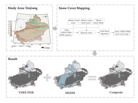
Snow Cover Mapping Based on SNPP-VIIRS Day/Night Band: A Case Study in Xinjiang, China

Institute of Remote Sensing and Geographic Information Systems, Peking University, 5 Summer Palace Road, Beijing 100871, China
*
Author to whom correspondence should be addressed.
Remote Sens. 2023, 15(12), 3004; https://0-doi-org.brum.beds.ac.uk/10.3390/rs15123004
Submission received: 26 April 2023
/
Revised: 30 May 2023
/
Accepted: 6 June 2023
/
Published: 8 June 2023
(This article belongs to the Special Issue Remote Sensing of Night-Time Light II)
Abstract
:Detailed snow cover maps are essential for estimating the earth’s energy balance and hydrological cycle. Mapping the snow cover across spatially extensive and topographically complex areas with less or no cloud obscuration is challenging, but the SNPP-VIIRS Day/Night Band (DNB) nighttime light data offers a potential solution. This paper aims to map snow cover distribution at 750 m resolution across the diverse 1,664,900 km2 of Xinjiang, China, based on SNPP-VIIRS DNB radiance. We implemented a swarm intelligent optimization technique Krill Herd algorithm, which finds the optimal threshold value by taking Otsu’s method as the objective function. We derived SNPP-VIIRS DNB snow maps of 14 consecutive scenes in December 2021, compared our snow-covered area estimations with those from MODIS and AMSR2 standard snow cover products, and generated composite snow maps by merging MODIS and SNPP-VIIRS DNB data. Results show that SNPP-VIIRS DNB snow maps are capable of providing reliable snow cover maps superior to MODIS and AMSR2, with an overall accuracy level of 84.66%. The composite snow maps at 500 m spatial resolution provided 55.85% more information on snow cover distribution than standard MODIS products and achieved an overall accuracy of 84.69%. Our study demonstrated the feasibility of snow cover detection in Xinjiang based on SNPP-VIIRS DNB, which can serve as a supplementary dataset for MODIS estimations where clouded pixels are present.
1. Introduction
Snow performs a prominent role in estimating the earth’s energy balance and hydrological cycle [1,2,3]. Heavy snowfalls and rapid snowmelt can result in economic damage and loss of life [4]. To effectively monitor these events, daily and accurate quantifications of snow-covered areas (SCA) are essential for tracking trends and changes in the spatial extent and duration of snow-covered land surfaces [1,5]. Additionally, snow depth (SD) measurements serve as auxiliary data for SCA estimation and could be obtained through remote sensing [6].
Various optical sensors have been developed for automated snow cover detection, including the Moderate Resolution Imaging Spectroradiometer (MODIS) on the Terra and Aqua satellites launched by NASA [7,8,9,10]. While MODIS provides daily snow cover maps at a moderate resolution of 500 m, it faces challenges, such as data gaps caused by cloud obscuration [1], degradation in accuracy over dense forest areas and shallow snow areas [7,11], and limited to daytime conditions [12,13].
The estimated accuracy of MODIS snow cover products is generally over 90% at locations worldwide [14]. However, these results were achieved mainly by overestimating cloud-contaminated pixels [5], which leaves a limited set of comparable data available for validation purposes and is more likely to achieve higher accuracy. Given that the mean cloud coverage of daily MODIS snow cover products is around 50% in Northern Xinjiang, China [9], cloud contamination is a severe impairment in applications of SCA mapping in Xinjiang solely based on MODIS snow products [15]. In contrast, passive microwave remote sensing can penetrate clouds and operate during the day and nighttime but offers a much lower spatial resolution [1,13]. As a result, microwave-based snow products are well suited for global snow mapping but are unable to resolve detailed landscape features of regional snow at a local scale of ≤1 km [1].
Nighttime light (NTL) data offers another approach to mapping SCA. Foster, in 1983, first implemented NTL for SCA detection using observations from the Defense Meteorological Satellite Program’s Operational Line-Scan System (DMSP-OLS) [16]. However, the use of DMSP-OLS data for SCA retrieval was limited due to its saturation effect and coarse spatial resolution [17]. The Visible Infrared Imaging Radiometer Suite (VIIRS) Day/Night Band (DNB) onboard the Suomi National Polar-orbiting Partnership (SNPP) launched in October 2011 overcomes these limitations [18,19]. The DNB is a panchromatic band that measures night lights and reflected solar (or lunar) lights at a spatial resolution of 750 m and captures an image twice a day, around 1:30 pm and 1:30 am local time. Within undeveloped and uninhabited regions with low or no artificial light source at the local crossing time of 1:30 am, VIIRS DNB data directly embodies the reflected lunar illuminance by the observed surface and indicates the presence of snow covers. Compared with conventional optical-based satellite observations, the advantages of mapping snow using NTL data include (1) the capability of retrieving SCA information under low-light conditions, particularly useful in areas with limited daytime hours due to high latitudes, or even perpetual nighttime conditions in the winters of the North and South Pole [20,21]; and (2) better data consistency (less cloud obscuration) because continental cloud coverage occurs less during nighttime compared to daytime [16,22]. In the current study focused on Xinjiang, the cloud coverage across the 14 consecutive scenes of VIIRS DNB during nighttime (~1:30 am) ranges from 3.07% to 49.04%, while the cloud coverage of MODIS (~10:30 am) ranges from 23.86% to 57.27%.
Following the launch of SNPP-VIIRS in 2011, Miller et al. [23] qualitatively demonstrated that the snow cover distribution details of a single VIIRS DNB imagery and a daytime VIIRS pass (true color) are consistent. Although this study provided evidence for the potential viability of VIIRS DNB for snow cover detection, the identification was based solely on visual interpretation and limited to a single pair of images.
Quantitative demonstrations of utilizing NTL on the retrieval of SCA were recently brought out by Huang et al. [21], in which a Minimum Error Thresholding algorithm was implemented for deriving SCA from VIIRS DNB data, with the accuracy of 80.3% and 76.7% for two case study areas, respectively. Additionally, this study highlighted the possibility of deriving accurate SCA maps with fewer data gaps by combining MODIS and VIIRS DNB imagery. So far, to the best of our knowledge, only this study has provided empirical evidence that combining MODIS and VIIRS DNB can map SCA accurately and thus require further affirmations. It is unclear if this approach can also achieve high-accuracy results for large areas and across a wider range of topographic characteristics.
In addition, Stopic and Dias [20] tested seven automated algorithms (i.e., Otsu, Li, Yen, triangle, minimum, mean, and Isodata) on four different case study areas (i.e., Colorado, USA; Ontario, Canada; Alaska, USA; Saskatchewan, Canada). To ensure the variety of multiple characteristics among the study areas, this study selected four regions with different traits in terms of latitudes, elevations, land cover types, and topographies. The results indicate that the higher overall accuracies achieved by the mean thresholding algorithm in Colorado and Alaska are attributed to their mountainous terrain features. Moreover, this study found that compared to MODIS, the VIIRS DNB snow extent tends to underestimate snow cover, which was explained by the presence of forest land covers. Although the effects of forests on the accuracy of snow detection are not surprising, it is important to note that the SCA estimations of MODIS substantially decrease over forested areas and shallow or patchy snow-covered surfaces. In other words, MODIS-derived SCA maps might not be the best dataset to take as “ground truth” reference maps. Lastly, the four study areas elected for examinations are all located in North America; hence they are insufficient to represent the spatial characteristics worldwide. This raises the question of whether these conclusions could transfer to Asia, particularly in Xinjiang, where an extensive variety of elevations, land cover types, and landforms are present.
Compared to the abovementioned snow maps generated from satellite observations through automated algorithms, the snow cover maps produced interactively with manual inputs by NOAA’S Interactive Multisensor Snow and Ice Mapping System (IMS) are a costly though highly reliable data source [5,24]. The production of IMS maps is dependent on visual interpretations by human analysts. Analysts are assigned to examine various available satellite imagery, automated snow mapping algorithms, and other ancillary data to map the snow distribution over clouds [25]. For a given pixel, when analysts do not have enough information to change the analysis, the IMS product for the present day is not updated, and the analysis from the previous day remains in effect [25]. This allows the IMS maps free of clouded pixels but makes the production of IMS maps time-consuming and expensive. However, these efforts have been proven to be valuable and worthwhile. Recent studies have shown that IMS maps of snow and ice are highly accurate and therefore are used as the reference data source for validations [26]. The consistency between the IMS product and in situ data has been evaluated by Chen et al. [26], who concluded a daily rate agreement of about 80–90% over the United States and southern Canada. Other validation results based on in situ measurements have shown an accuracy of over 90% in the Tibetan Plateau [27,28]. As all IMS SCA maps are obtained using the same procedure based on the same data source, it is within reason to postulate that the IMS SCA mapping is a reliable reference data for areas located in the northern hemisphere. Thus, in this study, we regarded IMS as the ground-truth reference data for accuracy assessment.
Accordingly, our study is placed in the context of the need for affirmations of automated snow cover mapping with VIIRS DNB data for large and topographically complicated areas in arid central Asia, particularly in Xinjiang, where the distribution of snow is of great importance. The main objectives of this study are to: (1) attempt a novel approach for the daily mappings of snow cover distribution utilizing VIIRS DNB data; (2) alleviate the data gaps of optical-based snow maps by providing snow cover information with the support of VIIRS DNB data, particularly in regions with frequent cloud obscurations and higher latitudes; and (3) reveal the strengths and short-comings of various snow mapping methods at a local scale.
2. Materials and Methods
2.1. Study Area
Xinjiang Uyghur Autonomous Region encompasses an area of ~1,664,900 km2, spanning ~1950 km from east to west and ~1550 km from north to south. Xinjiang is one of the most stable snow-covered areas in China, where the primary water resources rely heavily on snowmelt, and the effects of global warming are the most severe due to its semi-arid climate conditions [29]. Divided by the Tianshan Mountains, Xinjiang is separated into northern and southern portions. The Tianshan Mountains pose as a substantial obstacle to stable air flow and cause clouds and precipitation to form in Northern Xinjiang. A strong topographic contrast is present across Xinjiang (Figure 1). Studies have shown that under the effects of global warming, the mountainous terrain areas of Xinjiang, namely, Northern Xinjiang and the Tianshan Mountains, are undergoing a notable trend of precipitation changes [30,31,32] and variation in snow phenology [10]. Changes in snow coverage are related to regional climate conditions, water supplies, and natural disasters [33,34,35]. Therefore, studying the spatial variation of SCA in Xinjiang is of great importance.
2.2. Data Acquisition
2.2.1. Nighttime Light Data: SNPP-VIIRS DNB and Cloud Mask
The estimation of SCA through NTL relies on lunar illuminance levels [21]. The lunar phase is a commonly used proxy for lunar illuminance levels. Lunar phase refers to the fraction of illuminated moon surface visible to the observer and is formed by the relative positions of the earth, moon, and sun, often considered stable over a certain night. While lunar phase is commonly used for its convenience and straightforwardness, it has been proven to be a poor proxy, mainly because actual moonlight intensity on the ground does not show a simple correlation with it [36]. The lunar illuminance conditions of each day during the lunar month of December 2021 are given in Figure 2.
Aside from the lunar phase, the incident angle also has a prominent effect on lunar illuminance [36]. Recently, Śmielak proposed a model for estimating lunar illuminance, which significantly outperforms the lunar phase. This model succeeded in explaining 92% of the variation in the illuminance levels with a residual standard error of 1.4% [36]. The model considered five factors, namely, the relative moonlight intensity, the lunar disk brightness, the correction for the distance to the moon, the correction for atmospheric extinction, the correction for moon visibility, and the correction for the angle of incidence. Referring to this approach, we include the lunar elevation angle as one of the two measures for data filtering. The SNPP-VIIRS DNB data images utilized in this case study are filtered abiding by the following rules:
First, the lunar elevation angle has to exceed 10 degrees. Lunar illuminance increases notably when the moon is above the horizon [37] and is very likely to reach a peak value if and when the moon reaches the zenith due to light transmission mechanisms. However, the moon never reaches the zenith for locations beyond the latitude of 28°N/S worldwide [36]. In fact, every December, the lunar elevation angle reaches its local annual maximum value [37] of ~60 degrees in Xinjiang. The disparity of lunar illuminance over a year is larger in higher latitudes and decreases to almost zero on the equator [36]. Consistent with previous research [21], we chose to apply a threshold value of 10 degrees to indicate adequate lunar illuminance.
Second, cloud coverage has to be less than 60%. The actual lunar intensity on the ground varies with cloud coverage [36]. Generally, increasing cloud coverage would lead to a decrease in lunar illuminance levels due to the screening effect clouds have on downwelling radiation [37]. Conversely, cloud coverage might also result in increasing the ground lunar intensity levels because clouds tend to reflect more upwelling radiation. Following the first criterion, 14 scenes of SNPP-VIIRS DNB from the lunar cycle in December 2021 were extracted, spanning 15–28 December. We then examined the daily variation of cloud coverage in the corresponding MODIS scenes and found that the maximum cloud coverage of MODIS was 57.27%. For the sake of comparison, we settled on a likely threshold of 60% for cloud coverage in the selection of DNB scenes.
We found that the 14 consecutive days derived from the first criterion also met the second criterion. Thus, these 14 scenes were interpreted as available for snow cover detection (15–28 December). The acquired data product is the VIIRS Sensor Data Record Operational (JPSS VIIRS SDR), Version 1.3 product, which has gone through radiometric correction and georeferencing and can be freely accessed at the National Oceanic and Atmospheric Administration (NOAA) Comprehensive Large Array-data Stewardship System (CLASS), stored as the HDF-5 format [38]. All images in this study were reprojected into WGS 1984—UTM zone 45 N (EPSG: 32645) projection.
The SNPP-VIIRS L2 Cloud Mask is a product designed to sustain the long-term records of VIIRS [39]. This product contains both geophysical and geolocation data at a spatial resolution of 750 m. Frey et al. [15] demonstrated comparisons of this product against Cloud-Aerosol Lidar with Orthogonal Polarization (CALIOP) observations and evaluated hit rates of 90.0% for the 60°S–60°N land night from June through August 2018.
Additionally, we also acquired the monthly composite data of VIIRS DNB NTL data from Google Earth Engine Python API from January to December 2021.
2.2.2. Reference Data: IMS Snow Cover Extent
Since 2004, the IMS operated by NOAA National Environmental Satellite, Data, and Information Service (NESDIS) has been providing manually generated daily snow and ice cover maps for the Northern Hemisphere at three available resolutions (1 km, 4 km, and 24 km), spanning data from February 1997 to the present day. What is especially noteworthy is that this dataset is completely uncontaminated by clouds, owing to the use of multiple sources of satellite imagery, field data, and human analysts to discern snow cover from cloud cover.
In this paper, we collected the IMS maps for benchmarking the performance of VIIRS DNB snow extent estimates and the other two standard SCA products, MODIS and AMSR2. The 1 km IMS maps from 15 to 28 December 2021 were acquired from the National Snow and Ice Data Center (NSIDC) in the format of GeoTIFF [25].
2.2.3. Standard SCA Products: MODIS and AMSR2
Being one of the most prevalent data sources for SCA mapping, the MODIS suite of snow products includes global maps of SCA at a moderate resolution (500 m) and various temporal resolutions (daily, 8-day, 16-day, and monthly). We accessed the MODIS/Terra Snow Cover Daily L3 Global 500 m SIN Grid Version 6.1 dataset at the NSIDC repository [40] from 15–28 December 2021. In this study, six tiles of the MOD10A1 product (h23v04, h23v05, h24v04, h24v05, h25v04, and h25v05) were obtained for Xinjiang as our case study area.
The Advanced Microwave Scanning Radiometer 2 (AMSR2) was launched in 2012 onboard the Global Change Observation Mission First-Water satellite (GCOM-W1). We collected the GCOM-W1 AMSR2 Level 3 Snow Depth data via Globe Portal System (G-Portal), provided by the sensors on Earth Observation Satellites of Japan Aerospace Exploration Agency (JAXA). The selected dataset is at a spatial resolution of 10 km (0.1 deg), ascending orbit direction. We applied a thresholding value of 1 cm to convert the AMSR2 data from SD to SCA, corresponding with a previous study [6].
2.2.4. Auxiliary Data
We accessed the Landsat 8 Collection 1 Tier 1 Annual NDVI Composite dataset of 2021 derived from Landsat 8, distributed by Google Earth Engine, courtesy of the U.S. Geological Survey “https://developers.google.com/earth-engine/datasets/catalog/LANDSAT_LC08_C01_T1_ANNUAL_NDVI#terms-of-use (accessed on 5 June 2023)”.
The China lake dataset (1960s–2020) provided by the Tibet Plateau Data Center (TPDC) is a vector dataset in shapefile format, generated based on 4215 Landsat scenes and topographic maps [41]. This study used the 2020 subset of the China lake dataset as the data source for the extraction of water bodies. Table 1 lists the datasets used, the acquisition date, spatial resolution, and other measurement characteristics.
2.3. Methodology
The workflow for producing snow maps in this study included three steps: (1) Data Preparation, (2) NTL SCA Mapping, and (3) NTL and MODIS combined SCA Mapping. We then evaluated the produced snow maps through (4) cross-referenced assessments and (5) RMSE analyses. A conceptual map of the steps taken is given in Figure 3. The left column of Figure 3. focuses on the three production steps that are further described in Section 2.3.1, Section 2.3.2 and Section 2.3.3.
The right column of Figure 3. shows an example workflow of cross-referenced assessments and RMSE analyses when comparisons are between VIIRS DNB and IMS snow maps. In the workflow of cross-referenced assessment (Figure 3(4)), the left input branch is the dataset with a relatively finer resolution and needs to be resampled. Additionally, we also implemented McNemar’s statistical tests to find out whether DNB, MODIS, and AMSR2 maps are significantly divergent from each other. McNemar’s tests are completed based on cross-referenced assessments and do not require further image data processing; thus, we did not plot the workflow for this test in Figure 3. In the workflow of RMSE analyses (Figure 3(5)), the left input branch should be the dataset being evaluated (VIIRS DNB, MODIS, AMSR2, and Composite), while the right branch input is the reference dataset (IMS). These evaluation approaches are presented in Section 2.3.4, Section 2.3.5 and Section 2.3.6.
2.3.1. Data Preparation
The average DNB radiance of the daily VIIRS DNB data aggregated across Xinjiang increased significantly by several orders of magnitude on nights close to a full moon. Additionally, on such moonlit nights close to a full moon, the brighter surface radiance obtained from VIIRS DNB indicates snow cover. However, the brighter radiance of a given pixel could also be caused by the occurrence of clouds and artificial lights in urban areas.
To address cloud cover, we utilized the VIIRS integer cloud mask provided in the SNPP-VIIRS L2 Cloud Mask dataset. We located where the VIIRS integer cloud mask was marked as confidently cloudy to create a binary cloud mask.
Urban areas are illuminated by artificial lighting throughout the year and could be plotted using annual NTL data. In this study, urban areas were plotted based on the Vegetation Adjusted NTL Urban Index (VANUI) [42], as seen in Equation (1),
where is the obtained annual composite data, is the normalized DN value, calculated as follows (Equation (2)), where is the minimum DN value, and is the maximum DN value.
We calculated the annual VIIRS DNB imagery of 2021 by averaging monthly DNB images. Combined with the NDVI imagery of 2021, we generated the VANUI map of Xinjiang and performed a binary image segmentation using Otsu Algorithm to plot the urban areas (Figure 1). Apart from the masking of urban areas, pixels with anomalously high radiance (greater than that of the maximum annual radiance data within the urban areas) are considered outliers and removed as well.
Lastly, water body pixels should be masked before deriving the optimal threshold for snow cover detection. Most lakes in Xinjiang are frozen in December every year [43,44], and snow-covered ice lakes are not uncommon. As underlying surfaces inevitably factor in the reflectance of snow cover [45], snow-covered lake ice and snow-covered land might not exhibit the same level of reflectance. Moreover, when lake surfaces are not blanketed in snow, studies have shown that the radiance of pixels within and around water bodies is higher under moonlight due to the glint effect of water and (or) ice, also known as the light contamination effect [19]. Human activities, such as illegal fishing during nighttime, will also likely introduce errors within lakes [17,46]. Considering the above effects, we believe it necessary to mask water bodies away from DNB scenes. To obtain a binary water body mask, we converted the China lake dataset (2020) from vector to raster format, resampled it to 750 m, and extracted the pixels from the daily DNB radiance scenes. By doing this, we focus on the monitoring of snow-covered land surfaces, and any pixel with a radiance value below the derived optimal threshold would be identified as a snow-free land surface pixel.
2.3.2. NTL SCA Mapping: Krill Herd Algorithm
Among the many prevalent techniques for image segmentation based on bi-level thresholding, Otsu’s method is proved to be one of the most propitious objective functions [47,48]. The Krill Herd (KH) Algorithm [47] is a swarm intelligent optimization technique which finds the optimal value for an objective function while satisfying certain constraints. The objective function is normally implemented as conventional threshold-based image segmentation methods, such as Otsu’s [49] or Kapur’s method [50]. The KH algorithm was first proposed by Gandomi et al. in 2012 [51] and was later on tested in many studies that proved its main strengths in a better convergence speed when dealing with multilevel thresholding problems. A comparison of image segmentation based on KH-Otsu and Otsu was demonstrated by Geng et al. [52]. Their results showed that when performing double-threshold image segmentation, the number of iterations of Otsu segmentation increases exponentially, whereas, with the KH-Otsu algorithm, the number of iterations and execution time improves notably.
The KH algorithm takes inspiration from the behavior of krill swarms, where every individual krill’s herding behavior is dependent upon two factors: the density of krill and the concentration of food. In other words, the objective function is defined as a combination of the distance from the food and from the highest density of the krill swarm [47]. Meanwhile, the kth movement of the ith krill individual is depicted as three separate motions: (1) Movement induced by other krill individuals; (2) Foraging activity; and (3) Random diffusion. The time-dependent position of the ith krill is as seen in Equation (3).
where is the movement induced by other krill individuals, is the foraging activity, and is the random physical diffusion effect.
The movement induced by other krill individuals is considered because krills always intend to maintain a high density. For the kth movement of the ith krill, this effect could be denoted as Equation (4):
where represent the maximum guided speed, is the guided direction, is the previous motion speed, and is the inertia weight associating between and , which represents the tendency of staying the same, ranging from 0 to 1. The guided direction could be estimated from the local guidance effect induced by neighboring krills , and the target guidance effect induced by the optimal krill in the current population , as seen in Equation (5),
Foraging activity is the movement induced by two main factors: the food location, and the previous experience the previous food location provided, as seen in Equation (6),
where is the foraging speed, is the source of attraction of the foraging movement, represents the previous foraging movement, and is the inertia weight associating between and , which represents the tendency of staying the same, and ranges from 0 to 1. The source of attraction of the foraging movement is defined as Equation (7),
where is the food attraction perceived by the ith krill, and represents the attraction effect of the ith krill’s best fitness in previous locations. The random physical diffusion effect is a random process expressed by the maximum diffusion speed and the current random directional vector , as shown in Equation (8), where is the actual iteration number and is the maximum iteration number:
The KH algorithm is implemented in the following steps: (1) Initialization of KH parameters (, , , , and the initial population position of krills ); (2) Fitness evaluation of every krill individual in its initial position based on objective function; (3) Motion calculation given in Equation (3); (4) Genetic operators for reproduction; and (5) Update krills’ positions and fitness values. Detailed illustrations of the KH algorithm can be found in [51].
For each given VIIRS DNB image, an optimal threshold for the segmentation of snow and non-snow pixels is obtained, forming 14 days of SCA mapping. The source code of the KH algorithm and Otsu thresholding technique were both obtained from MathWorks [49,51]. Pixel-based evaluations, including cross-referenced assessments, McNemar tests, and RMSE analyses, were brought out for the snow cover extent extracted by this procedure and the standard snow cover maps of MODIS and AMSR2.
2.3.3. NTL and MODIS Combined SCA Mapping
As mentioned above, the main drawbacks of MODIS snow cover products are data gaps caused by cloud covers and the limited operating conditions (daytime). Multiple solutions to these issues have been brought out. Combining multiple daily observations is an approach that has been put into practice successfully (e.g., the 8-day composite MODIS snow cover data). Although this approach improves snow mapping accuracy and circumvents the cloud obscuration problem, it is achieved at the expense of temporal resolution [1].
In contrast, merging optical-based and microwave-based snow products provides a method for removing cloud obscurations while preserving spatial and temporal resolutions [12,13]. However, this approach is often unsatisfactory in cases where cloud coverage is too high, which might introduce errors through the rough spatial resolution of the microwave-based data [12,13]. As the DNB snow maps offer a much higher resolution (750 m) than microwave-based data (≥10 km), an alternative approach for an improved SCA interpretation is combining snow maps of MODIS with VIIRS-DNB. In this study, we used band math to substitute the clouded pixels of MODIS with the snow cover distribution of VIIRS DNB maps and produced composite snow maps of 500 m for Xinjiang. To validate this approach, we conducted cross-referenced assessments, McNemar statistical tests, and RMSE analyses, all of which will be described in Section 2.3.4, Section 2.3.5 and Section 2.3.6.
2.3.4. Cross-Referenced Assessment
In this section, we compared the SCA mappings derived from DNB nighttime light data with two standard snow cover products, namely, MODIS and AMSR2. The DNB, MODIS, and AMSR2 daily snow maps (14 scenes for each dataset) were all separately cross-referenced to the IMS daily maps, providing a statistical analysis of a range of metrics, including overall accuracy, F-1 score, precision, recall, false positives, and false negatives.
Within each pair of scenes for cross-referenced assessment, the scene with the relatively finer resolution was resampled to the spatial resolution of the other. Then, we calculated the union set of the urban and water body mask from each of the two scenes, and this union set was masked away mutually in both scenes. In other words, we removed the urban and water body pixels from consideration, leaving only pixels marked as either snow-covered, snow-free, or clouded for a session of cross-referenced assessment. A confusion matrix was calculated in each session of assessment, in which the two rows represent the classified outcomes of the predicted dataset (DNB, MODIS, AMSR2, or the composite maps), and the two columns represent the classified outcomes of the ground-truth dataset (IMS). Thus, we can calculate the number of pixels classified correctly as snow (true positive, TP) or snow-free (true negative, TN) and the pixels falsely classified as snow (false positive) or snow-free (false negative). Based on these four measures, we derived the overall accuracy, F-1 score, precision, recall, false positive rates, and false negative rates for each pair of scenes.
In addition, we slightly altered the terminology of false negatives (FN) to take into account the effects of cloud obscurations. Specifically, we denoted FN as the number of pixels that the assessed dataset misclassified as either snow-free or clouded. Based on these four measures, we also obtained the same range of metrics.
2.3.5. McNemar’s Statistical Test
McNemar’s test [53] is a statistical test to analyze the differences between two prediction datasets used on non-parametric paired nominal data with a dichotomous trait. In this study, McNemar’s test is applied to a 2 2 contingency table which includes the pixels correctly and incorrectly classified by the two datasets, using IMS maps as ground-truth reference data. The null hypothesis is that there are no significant differences between the two given datasets and that the two marginal probabilities for each classified outcome are the same, i.e.,
where is the number of samples correctly identified by both datasets, is the number of samples identified correctly exclusively by the first dataset, is the number of samples identified correctly exclusively by the second dataset, and is the number of samples incorrectly identified by both datasets. Both Equations (9) and (10) indicate:
Thus, estimating the McNemar with one degree of freedom using Equation (12) would offer us information on whether the null hypotheses can be assured or rejected.
For instance, to conduct a McNemar test between two selected prediction datasets, we first resampled them into the coarser resolution of the two datasets. We then intersected the areas where both prediction datasets provide snow distribution information. This approach removes urban, water body, and clouded pixels, leaving only snow-covered and snow-free pixels for paired examination. We then calculated with one degree of freedom using Equation (12). If the McNemar exceeds the critical value of with one degree of freedom, 3.84, then the null hypotheses can be rejected, signaling a significant statistical difference in the accuracy of the two selected datasets. In this case, if , then it could be concluded that the first dataset shows significantly better results than the second dataset, and vice versa.
A significant statistical difference between DNB and MODIS datasets is desirable since this indicates that DNB and MODIS are complementary to each other, which supports our approach of combining DNB with MODIS to produce composite maps. We performed McNemar tests upon 42 pairings of the snow maps of DNB, MODIS, and AMSR2 (14 days of 3 pairs of prediction datasets: DNB versus MODIS, DNB versus AMSR2, and MODIS versus AMSR2).
2.3.6. RMSE Analyses
Another way to describe the correspondence between predicted values and ground-truth values is by estimating the Root Mean Square Errors (RMSE). We calculated the daily RMSE values (Equation (13)) of VIIRS DNB, MODIS, and AMSR2, using IMS daily maps as reference data, spanning 15–28 December.
In Equation (13), was the number of pixels, and and were estimated and referenced data, respectively. In this study, each pixel was estimated as either snow-free (assigned 0) or snow-covered (assigned 1); thus, the RMSE values are dimensionless as they only describe the correspondence of snow cover spatial distribution between what was predicted and what was observed.
We also calculated the relative measure of RMSE (RRMSE) by dividing RMSEs with the average SCA values of referenced data using Equation (14),
in which was calculated following Equation (13), where was the number of days, and and were daily estimated and referenced SCA values, respectively.
3. Results
3.1. SCA Mapping in Xinjiang
As mentioned in Section 2.3.1 and Section 2.3.2, snow cover maps at 750 m spatial resolution across Xinjiang, spanning 15–28 December 2021, were derived based on the KH algorithm and daily DNB nighttime light images. By combining DNB and MODIS snow maps using the method described in Section 2.3.3, we obtained the daily composite data of snow distribution in Xinjiang.
Figure 4a–e shows the snow distribution in Xinjiang based on VIIRS DNB, AMSR2, MODIS, IMS, and the composite map. Overall, the large spatial variability of snow distribution is captured in all four datasets. Large snow patches are mainly distributed in Northern Xinjiang and the Kunlun Mountains. Across Xinjiang, extensive snow cover could be detected in Altay Mountains, Ili River Valley, Tianshan Mountains, Altun Mountains, and Kunlun Mountains, while the main snow-free regions are Tarim Basin, Junggar Basin, and Yiwu County. The distribution of snow in Northern Xinjiang is more evenly and continuous, scoring higher SCA values, while in Southern Xinjiang, the distribution of snow tends to be more incoherent, presenting lower SCA values.
To reflect the amount of snow cover information that can be provided in each dataset, we obtained the average snow and cloud coverage of VIIRS DNB, MODIS, AMSR2, IMS, and the composite maps from 15th to 28th December (Table 2).
Despite the similar spatial characteristics among these five datasets (Figure 4), cloud coverage loomed the largest in MODIS (on average 42.21%), which considerably limited its spatial extent for SCA mapping. The results also suggest that among VIIRS DNB, MODIS, and AMSR2, the SCA values obtained using VIIRS DNB data are the closest to those of IMS maps. Furthermore, the results of Table 2 show that the composite data maps provided much lower cloud coverage (11.15%) than standard MODIS snow maps (42.21%), alleviating the data gaps of MODIS that were caused by cloud obscuration. The mean value of the cloud-covered area dropped markedly from 6.91 to 1.83 × 10⁵ km2 (Figure 5). Meanwhile, the mean value of SCA increased considerably from 2.66 to 4.54 × 10⁵ km2 (Table 2). Pixels available for providing snow cover distribution, namely the sum of snow-free pixels and snow-covered pixels, increased in all 14 days, with an average increasing percentage of 55.85% and approximately 46.57% on the full moon night.
3.2. Cross-Referenced Assessment
As described in Section 2.3.4, we conducted two types of cross-referenced assessments for all four predicted datasets, and the results are given in Table 3 and Table 4.
During cross-referenced assessments with clouded pixels omitted (Table 3), we found that over the whole course of the selected 14 days, VIIRS DNB and the composite maps substantially outperformed AMSR2 almost every day. However, when compared to MODIS (86.21%), the average overall accuracies of DNB (84.66%), and the composite maps (84.69%) were lower than MODIS by approximately 2%.
Moreover, DNB maps scored the highest precision and lowest false positive rates, while MODIS maps scored the highest recall and lowest false negative rates (Table 3). The composite maps exhibited the highest F-1 score among the four predicted datasets. Under this method of assessment, AMSR2 proved to be the least competent among all four datasets.
After expanding the definition of false negative pixels by including misclassified clouded pixels, our results (Table 4) showed that the highest overall accuracy and F-1 score were achieved by the composite maps, closely followed by DNB and AMSR2. Showing remarkable contradictions to the results in Table 3, under this assessment, MODIS scored the lowest overall accuracy and F-1 score. Although DNB, MODIS, and the composite maps all showed a decrease in Table 4 compared to Table 3, the performances of MODIS dropped the most dramatically. AMSR2 maps are uncontaminated by clouds. Hence, all six metrics of the AMSR2 dataset remained the same as in Table 3. Additionally, since this approach only affected the FN values of each dataset, the precision, and false positive rates under this method (Table 4) remained the same as in Table 3.
We also plotted the daily variation of the overall accuracy when clouded pixels were omitted or included (Figure 6).
A decrease in accuracy was found on 21 December for both types of cross-referenced assessments because of sizable cloud coverage in MODIS, DNB, and composite datasets on this day (54.66%, 49.04%, and 32.99%, respectively). Moreover, as seen in Figure 6a, when clouded pixels were omitted, VIIRS DNB only slightly outperformed MODIS during 17–25 December (VIIRS DNB: overall accuracy 87.92%, F-1 score 0.8045; MODIS overall accuracy: 87.17%, F-1 score 0.7726). The occurrence of a full moon on 19th December is likely accountable for the preferable performances on 17–25 December of VIIRS DNB. Aside from these statistics, it is also crucial to consider the area available for performing cross-referenced assessments when clouded pixels were omitted (Table 5).
Overall, the composite maps provided the most extensive area for cross-referenced assessments, exceeding AMSR2. This is because although AMSR2 is uncontaminated by clouds, the path of the satellite orbit prevents it from collecting Xinjiang’s full coverage data in a single overpass (Figure 4b). Hence, in Table 5, the area available for cross-referenced assessment between AMSR2 and IMS varies within the 14 scenes, presenting a maximum of 94.79% coverage across the whole area of Xinjiang in a single scene. Although combining the ascending and descending overpassing scenes collected by AMSR2 would easily provide full daily coverage of Xinjiang, we only utilized the ascending scene. The reason is that implementing different algorithms for the combination of ascending and descending scenes would introduce additional uncertainties and greatly influence the outcome performances, which is not the main focus of this paper.
3.3. McNemar’s Statistical Test
To check if DNB and MODIS maps are complementary to each other, we carried out a McNemar’s test (DNB versus MODIS) and hope to discover a statistically significant difference in DNB and MODIS. This test was also applied to DNB versus AMSR2, and MODIS versus AMSR2, to gain more insight into the performances of each independently predicted dataset. The minimum, maximum, and average statistics of daily test results in each set of comparisons were derived and presented in Table 6.
As mentioned in Section 2.3.5, the critical value of at 95% confidence is 3.84. In each pair of datasets for comparison, the common logarithm of exhibited larger values than the common logarithm value . This indicated a statistically significant difference in the spatial distribution of incorrectly classified pixels among DNB, MODIS, and AMSR2.
In Table 6, the values were consistently higher than in each set of comparison. The sub-column of within each pair of datasets in comparison denotes the number of pixels where Dataset 1 predicted correctly while Dataset 2 did not. Thus, Table 6 suggested a significant superiority of DNB to both MODIS and AMSR2. Likewise, MODIS was also proved to be significantly more accurate than AMSR2.
3.4. RMSE Analyses
The daily RMSEs of VIIRS DNB, MODIS, AMSR2, and the composite maps compared with IMS maps are shown below in Table 7.
Lower RMSE values generally imply more precise predictions. In Table 7, the composite maps achieved the lowest mean RMSE, closely followed by MODIS and VIIRS DNB maps, and lastly, the AMSR2 dataset offered the highest RMSE values. These results are consistent with the clouded pixels omitted cross-referenced assessment results of Table 3, where VIIRS DNB, MODIS, and the composite maps achieved a similar level of overall accuracy and F-1 Score results that were superior to AMSR2. We plotted the daily variation of DNB radiance alongside RMSE in Figure 7, which shows a general decrease in RMSE and an increase in DNB radiance when close to the full moon occurrence. These tendencies are similar to those of the cross-referenced results in Section 3.2 (Figure 7).
We derived the RRMSEs of the composite and MODIS maps (Figure 8) using the method described in Section 2.3.6. In contrast to the dimensionless RMSEs in Table 7 and Figure 7, the RMSE values in Figure 8 represent the difference in SCA values detected by MODIS and the composite maps in the units of km2. Meanwhile, RRMSEs are dimensionless and represent the relative differences between estimated (MODIS or composite maps) and expected (IMS maps) SCA values. The SCA values of the composite data maintained an agreeable linearity with IMS maps (Figure 8). In this study, we consider model accuracy to be excellent when RRMSE < 10%, good when 10% < RRMSE < 20%, fair if 20% < RRMSE < 30%, and poor if RRMSE exceeds 30% [54,55]. According to the performance of 10.58% in RRMSE, the composite data was in close proximity to excellent accuracy.
4. Discussion
4.1. SCA Mapping Based on SNPP-VIIRS DNB
The VIIRS DNB nighttime light snow maps generated in this study performed well in demonstrating the spatial pattern of snow cover distributed across the topographically complex Xinjiang and agree well with previous research [10,13,56]. However, as seen in Table 2, the average SCA detected by DNB (3.5513 × 10⁵ km2) was significantly lower than the SCA mapped by IMS (5.9285 × 10⁵ km2). Aside from the influence of clouds, another major reason for the difference is the snow cover in urban areas. IMS maps can provide snow distribution information over urban areas in Xinjiang, while the SCA mapping in this study does not apply to urban areas. This is because the differentiation of artificial illumination and the moonlight reflected by snow cover in urban areas is yet an unresolved challenge, and so urban areas were masked away as noise pixels in data preparation.
For pixel-based accuracy assessments, DNB, MODIS, and AMSR2 were separately compared against the daily IMS maps from 15 to 28 December using cross-referenced assessments, McNemar’s tests, and RMSE analyses.
We found that when clouded pixels were omitted for cross-referenced assessments (Table 3), the overall accuracies of VIIRS DNB (84.66%) were lower than MODIS (86.21%) over the whole course of the selected 14 days with adequate lunar illuminance. We also found that VIIRS DNB (87.92%) only slightly outperformed MODIS (87.17%) from 17th to 25th December (Figure 6a). Furthermore, our evaluation of the relationship between RMSE and average DNB radiance (Figure 7) demonstrated a negative correlation. These results strongly suggest that although the criteria given in Section 2.2.1 worked well when selecting data for reliable snow detection, to achieve an overall accuracy as high as MODIS, sufficient lunar illuminance is required. Owing to the fact that the vast majority of snow is distributed in the peaks and foothills of mountains, when the lunar elevation angle is low, the lunar illuminance is insufficient to support the accurate mapping of SCA.
Our cross-referenced results (Table 3 and Table 4) also showed that AMSR2 maps tend to underestimate the snow cover distribution in Xinjiang. This underestimation of snow cover could be potentially explained by the coarse spatial resolution of 10 km, which is too coarse for the mapping of SCA at the landscape level. Furthermore, the false negatives were considerably and consistently higher than false positives, for all three independent datasets (i.e., VIIRS DNB, MODIS, and AMSR2). This corroborates with previous findings [20], where the difference between false positives and false negatives was explained by the underestimation of snow extent by the VIIRS DNB data. False negatives occur when pixels are incorrectly classified as snow-free, signaling an underestimation of snow cover. Stopic and Dias explained this underestimation of snow extent by the presence of open and closed evergreen needle leaf forests [20]. Many studies have demonstrated that because below-canopy snow covers are often present in mixed pixels, they are commonly misclassified as snow-free in pixel-based optical snow mapping, causing an underestimation of snow cover over forested areas [1,14,57,58]. For this reason, there is a very high probability that forested pixels of the mountainous areas are partly accountable for the high false negative rates for DNB, MODIS, and AMSR2 datasets in this study.
Although our cross-referenced results (Table 3) showed that MODIS yielded a higher overall accuracy over DNB, we believe that VIIRS DNB provided more reliable estimations of SCA. First, it is more likely to achieve better results when fewer pixels are available for cross-referenced assessment, and DNB was able to provide an average of 80.84% area available for assessment, while MODIS provided only 57.62% (Table 5). Second, during McNemar’s tests, we found more pixels misclassified by MODIS while correctly classified by DNB than the reverse condition (Table 6). This signifies that when DNB and MODIS both can provide snow cover distribution information, DNB is more in agreement with the ground-truth IMS dataset than MODIS.
However, a hindrance in mapping SCA with DNB data is the limited temporal availability. Only around 14 nights in each month have adequate lunar illuminance for snow cover detection, and according to our findings, only 9 consecutive nights demonstrated a similar level of performance to that of MODIS. In other words, this data might not be suitable for long-term sequential daily observations of SCA.
Moreover, high-order scattering effects caused by terrain features over hilly and mountainous areas intensify the reflection of moonlight per se, regardless of their snow cover distribution [19]. This affects the radiance of VIIRS data fundamentally and consequently influences the reliability of snow detection in mountainous regions when applying threshold-based image segmentation techniques.
In summary, estimating daily SCA values by utilizing VIIRS DNB nighttime light data is an attainable and reliable approach. In the near future, to further highlight the strengths of this approach, we propose using this method to produce snow maps during polar nights, when daytime observations by MODIS are ineffective.
4.2. Composite SCA Mapping with MODIS and SNPP-VIIRS DNB
VIIRS DNB can act as supplements to MODIS SCA estimations, by providing invaluable information for clouded pixels in MODIS scenes. Spatial disparities between DNB and MODIS are beneficial when them to obtain composite maps. The results from cross-referenced assessments indicated that DNB and MODIS are complementary to each other. When clouded pixels were omitted (Table 3), DNB presented better performances in precision (86.11%) and false positive rate (6.11%) than MODIS (precision 74.17%, false positive rate 9.58%). Meanwhile, DNB exhibited a lower recall (66.43%) and higher false negative rate (33.57%) than MODIS (recall 74.65%, false negative rate 25.35%). These results suggest that compared to MODIS, DNB snow maps are less likely to misclassify snow-free pixels as snow-covered pixels, and more likely to misclassify snow-covered pixels as snow-free pixels.
To further check if DNB and MODIS data are complementary to each other, we conducted a series of McNemar’s statistical tests. Our results (Table 6) proved that the spatial distribution of misclassified pixels in DNB and MODIS were statistically divergent. In other words, when a certain pixel is misclassified by one of the two datasets, it is very likely to be correctly classified by the other.
Another reason combining DNB and MODIS is beneficial, is that cloud obscuration is a serious concern in snow cover mapping for optical sensors operating in daytime. Cloud obscuration largely limits their applications in SCA predictions for larger areas, such as Xinjiang. In this regard, VIIRS DNB presents an advantage of offering snow maps with much lower cloud coverage than MODIS because continental cloud coverage is less during nighttime than daytime [22]. The average cloud coverage (Table 2) of MODIS snow maps in this study was as high as 42.21% over the selected 14 days, which agrees with previous findings [9,59]. In contrast, 18.87% of the area across Xinjiang was obscured by clouds in DNB, and even less in composite maps (11.15%). The low cloud coverage of composite maps resulted in 55.85% more area for snow cover mapping.
The effects of cloud obscuration on each dataset were also implied through the cross-referenced assessments (Table 3 and Table 4). After the term ‘false negative’ was expanded to the number of pixels where IMS marked as snow-covered while MODIS marked as cloud-covered or snow-free, the overall accuracy of MODIS dropped drastically from the best (85.21%) to the worst (63.44%) among the four predicted datasets. In contrast, the performances of DNB maintained an overall accuracy of well over 75%. In Table 3 and Table 4, the composite maps provided desirable overall accuracy and F-1 score results. By alleviating the data gaps from MODIS, the composite maps provided a higher precision than MODIS, a higher recall than DNB, about the same level of the false positive rate as MODIS, and a lower false negative rate than DNB. The improvements in recall and precision were reflected through the high F-1 scores (0.7592 and 0.6969) of the composite data, the highest among all four predicted datasets. Additionally, the RRMSE evaluations of the composite maps (Figure 8) demonstrated strong and positive linearity with IMS maps, which confirms the superiority of the composite maps to MODIS.
It is also worth mentioning some limitations to composite SCA mapping. Our method of replacing clouded pixels from MODIS with the corresponding pixels from DNB data inevitably allows all false positive errors in the MODIS scenes to directly propagate into the composite maps. Consequently, in both Table 3 and Table 4, the composite maps yielded a similar level of false positive rates to MODIS.
Although composite maps offer desirable cross-referenced results, some underlying assumptions in this study are very likely a source of uncertainty in the estimation of SCA. During the combination of DNB and MODIS maps, the clouded pixels of MODIS were directly replaced by the snow distribution in DNB, despite the slight temporal differences in data acquisition between these two datasets. Freshly fallen snow observed during the daytime by Terra-MODIS could melt before the following nighttime observation by SNPP-VIIRS DNB. Thus, the assumption that the diurnal changes of snow distribution on a local scale are negligible, is partly accounted for the errors of the composite SCA maps.
5. Conclusions
This paper presented an approach for obtaining nighttime SCA maps over large areas with diverse topography conditions in Xinjiang, based on VIIRS DNB nighttime light data. We demonstrated the utility of snow cover detection, and of combining daily VIIRS DNB measures with MODIS snow maps to map SCA across ~1,664,900 km2 of Xinjiang Province. Our method yielded reliable SCA estimations that outperformed AMSR2 snow cover products.
The overall accuracy of our SCA predictions was satisfactory though not outstanding when compared to MODIS. However, the ability to provide more snow distribution information is invaluable, and therefore, VIIRS DNB serves well as a complementary dataset for MODIS snow maps.
The results of this work motivate future research focused on improving SCA mapping based on VIIRS DNB and MODIS to introduce certain temporal corrections before combining the observations from these two datasets. Additionally, in situ observations of SCA from meteorological stations are indispensable for higher credibility in data validation. Furthermore, a long-term case study is essential to confirm the feasibility of improving MODIS snow cover mapping by integrating VIIRS DNB data. We also propose using this method to produce snow maps during polar nights, when daytime observations by MODIS are ineffective.
Author Contributions
Data processing, implementation and draft preparation, B.C.; funding acquisition, conceptualization, and review and editing, X.Z.; data curation, M.R.; algorithm implementation, X.C.; and statistic test, J.C. All authors have read and agreed to the published version of the manuscript.
Funding
This research was funded by National Natural Science Foundation of China, grant number 42171327.
Data Availability Statement
See Section 2.2 for information about how to access the data used in this study.
Conflicts of Interest
The authors declare no conflict of interest.
References
- Dietz, A.J.; Kuenzer, C.; Gessner, U.; Dech, S. Remote sensing of snow—A review of available methods. Int. J. Remote Sens. 2011, 33, 4094–4134. [Google Scholar] [CrossRef]
- Che, T.; Dai, L.; Zheng, X.; Li, X.; Zhao, K. Estimation of snow depth from passive microwave brightness temperature data in forest regions of northeast China. Remote Sens. Environ. 2016, 183, 334–349. [Google Scholar] [CrossRef]
- Nayak, A.; Marks, D.; Chandler, D.G.; Seyfried, M. Long-term snow, climate, and streamflow trends at the Reynolds Creek Experimental Watershed, Owyhee Mountains, Idaho, United States. Water Resour. Res. 2010, 46, 1–15. [Google Scholar] [CrossRef]
- Cousins, K. The Economic Benefits and Costs of Snow in the Upper Colorado Basin; Earth Economics: Tacoma, WA, USA, 2017. [Google Scholar]
- Kongoli, C.; Romanov, P.; Ferraro, R. Snow Cover Monitoring from Remote-Sensing Satellites: Possibilities for Drought Assessment. In Remote Sensing of Drought: Innovative Monitoring Approaches; CRC Press: Boca Raton, FL, USA, 2012; Volume 554, pp. 359–385. [Google Scholar]
- Bian, Q.; Xu, Z.; Zheng, H.; Li, K.; Liang, J.; Fei, W.; Shi, C.; Zhang, S.; Yang, Z.L. Multiscale Changes in Snow Over the Tibetan Plateau During 1980–2018 Represented by Reanalysis Data Sets and Satellite Observations. J. Geophys. Res. Atmos. 2020, 125, 1–17. [Google Scholar] [CrossRef]
- Ault, T.W.; Czajkowski, K.P.; Benko, T.; Coss, J.; Struble, J.; Spongberg, A.; Templin, M.; Gross, C. Validation of the MODIS snow product and cloud mask using student and NWS cooperative station observations in the Lower Great Lakes Region. Remote Sens. Environ. 2006, 105, 341–353. [Google Scholar] [CrossRef]
- Huang, X.; Liang, T.; Zhang, X.; Guo, Z. Validation of MODIS snow cover products using Landsat and ground measurements during the 2001–2005 snow seasons over northern Xinjiang, China. Int. J. Remote Sens. 2011, 32, 133–152. [Google Scholar] [CrossRef]
- Liang, T.; Huang, X.; Wu, C.; Liu, X.; Li, W.; Guo, Z.; Ren, J. An application of MODIS data to snow cover monitoring in a pastoral area: A case study in Northern Xinjiang, China. Remote Sens. Environ. 2008, 112, 1514–1526. [Google Scholar] [CrossRef]
- Wang, Q.; Ma, Y.; Li, J. Snow Cover Phenology in Xinjiang Based on a Novel Method and MOD10A1 Data. Remote Sens. 2023, 15, 1474. [Google Scholar] [CrossRef]
- Simic, A.; Fernandes, R.; Brown, R.; Romanov, P.; Park, W. Validation of VEGETATION, MODIS, and GOES+ SSM/I snow-cover products over Canada based on surface snow depth observations. Hydrol. Process. 2004, 18, 1089–1104. [Google Scholar] [CrossRef]
- Gao, Y.; Xie, H.; Lu, N.; Yao, T.; Liang, T. Toward advanced daily cloud-free snow cover and snow water equivalent products from Terra–Aqua MODIS and Aqua AMSR-E measurements. J. Hydrol. 2010, 385, 23–35. [Google Scholar] [CrossRef]
- Liang, T.; Zhang, X.; Xie, H.; Wu, C.; Feng, Q.; Huang, X.; Chen, Q. Toward improved daily snow cover mapping with advanced combination of MODIS and AMSR-E measurements. Remote Sens. Environ. 2008, 112, 3750–3761. [Google Scholar] [CrossRef]
- Hall, D.K.; Riggs, G.A. Accuracy assessment of the MODIS snow products. Hydrol. Process. 2007, 21, 1534–1547. [Google Scholar] [CrossRef]
- Frey, R.A.; Ackerman, S.A.; Holz, R.E.; Dutcher, S.; Griffith, Z. The Continuity MODIS-VIIRS Cloud Mask. Remote Sens. 2020, 12, 3334. [Google Scholar] [CrossRef]
- Foster, J.L. Night-time observations of snow using visible imagery. Int. J. Remote Sens. 1983, 4, 785–791. [Google Scholar] [CrossRef]
- Levin, N.; Kyba, C.C.M.; Zhang, Q.; Sánchez de Miguel, A.; Román, M.O.; Li, X.; Portnov, B.A.; Molthan, A.L.; Jechow, A.; Miller, S.D.; et al. Remote sensing of night lights: A review and an outlook for the future. Remote Sens. Environ. 2020, 237, 111443. [Google Scholar] [CrossRef]
- Hillger, D.; Seaman, C.; Liang, C.; Miller, S.; Lindsey, D.; Kopp, T. Suomi NPP VIIRS Imagery evaluation. J. Geophys. Res. Atmos. 2014, 119, 6440–6455. [Google Scholar] [CrossRef]
- Wang, Z.; Román, M.O.; Kalb, V.L.; Miller, S.D.; Zhang, J.; Shrestha, R.M. Quantifying uncertainties in nighttime light retrievals from Suomi-NPP and NOAA-20 VIIRS Day/Night Band data. Remote Sens. Environ. 2021, 263, 112557. [Google Scholar] [CrossRef]
- Stopic, R.; Dias, E. Examining Thresholding and Factors Impacting Snow Cover Detection Using Nighttime Images. Remote Sens. 2023, 15, 868. [Google Scholar] [CrossRef]
- Huang, Y.; Song, Z.; Yang, H.; Yu, B.; Liu, H.; Che, T.; Chen, J.; Wu, J.; Shu, S.; Peng, X.; et al. Snow cover detection in mid-latitude mountainous and polar regions using nighttime light data. Remote Sens. Environ. 2022, 268, 112766. [Google Scholar] [CrossRef]
- Dong, X.; Minnis, P.; Xi, B. A Climatology of Midlatitude Continental Clouds from the ARM SGP Central Facility: Part I: Low-Level Cloud Macrophysical, Microphysical, and Radiative Properties. J. Clim. 2005, 18, 1391–1410. [Google Scholar] [CrossRef] [Green Version]
- Miller, S.; Straka, W.; Mills, S.; Elvidge, C.; Lee, T.; Solbrig, J.; Walther, A.; Heidinger, A.; Weiss, S. Illuminating the Capabilities of the Suomi National Polar-Orbiting Partnership (NPP) Visible Infrared Imaging Radiometer Suite (VIIRS) Day/Night Band. Remote Sens. 2013, 5, 6717–6766. [Google Scholar] [CrossRef] [Green Version]
- Chiu, J.; Paredes-Mesa, S.; Lakhankar, T.; Romanov, P.; Krakauer, N.; Khanbilvardi, R.; Ferraro, R. Intercomparison and Validation of MIRS, MSPPS, and IMS Snow Cover Products. Adv. Meteorol. 2020, 2020, 4532478. [Google Scholar] [CrossRef]
- National Ice Center. IMS Daily Northern Hemisphere Snow and Ice Analysis at 1 km, 4 km, and 24 km Resolutions, Version 1; NASA National Snow and Ice Data Center, Distributed Active Archive Center: Boulder, CO, USA, 2008; updated daily. [Google Scholar]
- Chen, C.; Lakhankar, T.; Romanov, P.; Helfrich, S.; Powell, A.; Khanbilvardi, R. Validation of NOAA-Interactive Multisensor Snow and Ice Mapping System (IMS) by Comparison with Ground-Based Measurements over Continental United States. Remote Sens. 2012, 4, 1134–1145. [Google Scholar] [CrossRef] [Green Version]
- Yang, J.; Jiang, L.; Ménard, C.B.; Luojus, K.; Lemmetyinen, J.; Pulliainen, J. Evaluation of snow products over the Tibetan Plateau. Hydrol. Process. 2015, 29, 3247–3260. [Google Scholar] [CrossRef]
- Li, W.; Guo, W.; Qiu, B.; Xue, Y.; Hsu, P.C.; Wei, J. Influence of Tibetan Plateau snow cover on East Asian atmospheric circulation at medium-range time scales. Nat. Commun. 2018, 9, 4243. [Google Scholar] [CrossRef] [PubMed] [Green Version]
- Ye, L.; Grimm, N.B. Modelling potential impacts of climate change on water and nitrate export from a mid-sized, semiarid watershed in the US Southwest. Clim. Change 2013, 120, 419–431. [Google Scholar] [CrossRef]
- Hu, W.; Yao, J.; He, Q.; Chen, J. Changes in precipitation amounts and extremes across Xinjiang (northwest China) and their connection to climate indices. PeerJ 2021, 9, e10792. [Google Scholar] [CrossRef]
- Yao, J.; Chen, Y.; Zhao, Y.; Mao, W.; Xu, X.; Liu, Y.; Yang, Q. Response of vegetation NDVI to climatic extremes in the arid region of Central Asia: A case study in Xinjiang, China. Theor. Appl. Climatol. 2017, 131, 1503–1515. [Google Scholar] [CrossRef]
- Zhang, M.; Chen, Y.; Shen, Y.; Li, B. Tracking climate change in Central Asia through temperature and precipitation extremes. J. Geog. Sci. 2019, 29, 3–28. [Google Scholar] [CrossRef] [Green Version]
- Cohen, J.; Rind, D. The Effect of Snow Cover on the Climate. J. Clim. 1991, 4, 689–706. [Google Scholar] [CrossRef]
- Hui, R.; Zhao, R.; Liu, L.; Li, X. Effect of snow cover on water content, carbon and nutrient availability, and microbial biomass in complexes of biological soil crusts and subcrust soil in the desert. Geoderma 2022, 406, 115505. [Google Scholar] [CrossRef]
- Caretta, M.A.; Mukherji, A.; Arfanuzzaman, M.; Betts, R.A.; Gelfan, A.; Hirabayashi, Y.; Lissner, T.K.; Liu, J.; Lopez, G.E.; Morgan, R.; et al. Water. In Climate Change 2022: Impacts, Adaptation, and Vulnerability. Contribution of Working Group II to the Sixth Assessment Report of the Intergovernmental Panel on Climate Change; Pörtner, H.-O., Roberts, D.C., Tignor, M., Poloczanska, E.S., Mintenbeck, K., Alegría, A., Craig, M., Langsdorf, S., Löschke, S., Möller, V., et al., Eds.; Cambridge University Press: Cambridge, UK; New York, NY, USA, 2022; in press. [Google Scholar]
- Śmielak, M.K. Biologically meaningful moonlight measures and their application in ecological research. Behav. Ecol. Sociobiol. 2023, 77, 21. [Google Scholar] [CrossRef]
- Krieg, J. Influence of moon and clouds on night illumination in two different spectral ranges. Sci. Rep. 2021, 11, 20642. [Google Scholar] [CrossRef]
- National Centers for Environmental Information. Available online: https://www.ncei.noaa.gov/metadata/geoportal/rest/metadata/item/gov.noaa.ncdc%3AC00864/html (accessed on 5 June 2023).
- NASA Level1 and Atmosphere Archive & Distribution System (LAADS) Distributed Active Archive Center (DAAC). Available online: https://ladsweb.modaps.eosdis.nasa.gov/missions-and-measurements/products/CLDMSK_L2_VIIRS_SNPP/ (accessed on 5 June 2023).
- National Snow and Ice Data Center. Available online: https://nsidc.org/data/mod10a1/versions/61 (accessed on 5 June 2023).
- Zhang, G.; Yao, T.; Chen, W.; Zheng, G.; Shum, C.K.; Yang, K.; Piao, S.; Sheng, Y.; Yi, S.; Li, J.; et al. Regional differences of lake evolution across China during 1960s–2015 and its natural and anthropogenic causes. Remote Sens. Environ. 2019, 221, 386–404. [Google Scholar] [CrossRef]
- Zhang, Q.; Schaaf, C.; Seto, K.C. The Vegetation Adjusted NTL Urban Index: A new approach to reduce saturation and increase variation in nighttime luminosity. Remote Sens. Environ. 2013, 129, 32–41. [Google Scholar] [CrossRef]
- Jing, Y.; Zhang, F.; Wang, X. Monitoring dynamics and driving forces of lake changes in different seasons in Xinjiang using multi-source remote sensing. Eur. J. Remote Sens. 2018, 51, 150–165. [Google Scholar] [CrossRef] [Green Version]
- Cai, Y.; Ke, C.-Q.; Yao, G.; Shen, X. MODIS-observed variations of lake ice phenology in Xinjiang, China. Clim. Chang. 2020, 158, 575–592. [Google Scholar] [CrossRef]
- Wiscombe, W.J.; Warren, S.G. A Model for the Spectral Albedo of Snow. I: Pure Snow. J. Atmos. Sci. 1980, 37, 2712–2733. [Google Scholar] [CrossRef]
- Elvidge, C.; Zhizhin, M.; Baugh, K.; Hsu, F.-C. Automatic Boat Identification System for VIIRS Low Light Imaging Data. Remote Sens. 2015, 7, 3020–3036. [Google Scholar] [CrossRef] [Green Version]
- Baby Resma, K.P.; Nair, M.S. Multilevel thresholding for image segmentation using Krill Herd Optimization algorithm. J. King Saud Univ. Comput. Inf. Sci. 2021, 33, 528–541. [Google Scholar] [CrossRef]
- Pare, S.; Kumar, A.; Singh, G.K.; Bajaj, V. Image Segmentation Using Multilevel Thresholding: A Research Review. Iran. J. Sci. Technol. Trans. Electr. Eng. 2019, 44, 1–29. [Google Scholar] [CrossRef]
- Otsu, N. A Threshold Selection Method from Gray-Level Histograms. IEEE Trans. Syst. Man Cybern. 1979, 9, 62–66. [Google Scholar] [CrossRef] [Green Version]
- Kapur, J.N.; Sahoo, P.K.; Wong, A.K.C. A New Method for Gray-Level Picture Thresholding Using the Entropy of the Histogram. Comput. Vis. Graph. Image Process. 1985, 29, 273–285. [Google Scholar] [CrossRef]
- Gandomi, A.H.; Alavi, A.H. Krill herd: A new bio-inspired optimization algorithm. Commun. Nonlinear Sci. Numer. Simul. 2012, 17, 4831–4845. [Google Scholar] [CrossRef]
- Geng, Q.; Yan, H.; Kumar, V. Image Segmentation under the Optimization Algorithm of Krill Swarm and Machine Learning. Comput. Intell. Neurosci. 2022, 2022, 8771650. [Google Scholar] [CrossRef] [PubMed]
- McNemar, Q. Note on the sampling error of the difference between correlated proportions or percentages. Psychometrika 1947, 12, 153–157. [Google Scholar] [CrossRef]
- Despotovic, M.; Nedić, V.; Despotović, D.; Cvetanović, S. Evaluation of empirical models for predicting monthly mean horizontal diffuse solar radiation. Renew. Sustain. Energy Rev. 2016, 56, 246–260. [Google Scholar] [CrossRef]
- Li, M.-F.; Tang, X.-P.; Wu, W.; Liu, H.-B. General models for estimating daily global solar radiation for different solar radiation zones in mainland China. Energy Convers. Manag. 2013, 70, 139–148. [Google Scholar] [CrossRef]
- Chen, W.; Ding, J.; Wang, J.; Zhang, J.; Zhang, Z. Temporal and spatial variability in snow cover over the Xinjiang Uygur Autonomous Region, China, from 2001 to 2015. PeerJ 2020, 8, e8861. [Google Scholar] [CrossRef] [Green Version]
- Luo, J.; Dong, C.; Lin, K.; Chen, X.; Zhao, L.; Menzel, L. Mapping snow cover in forests using optical remote sensing, machine learning and time-lapse photography. Remote Sens. Environ. 2022, 275, 113017. [Google Scholar] [CrossRef]
- Nolin, A.W. Recent advances in remote sensing of seasonal snow. J. Glaciol. 2010, 56, 1141–1150. [Google Scholar] [CrossRef] [Green Version]
- Wang, X.; Xie, H.; Liang, T. Evaluation of MODIS snow cover and cloud mask and its application in Northern Xinjiang, China. Remote Sens. Environ. 2008, 112, 1497–1513. [Google Scholar] [CrossRef]
Figure 1.
Case study area: Xinjiang. Urban areas were plotted in the color magenta, based on annual DNB nighttime light data: (1) Karamay, (2) Fule, (3) Yining, (4) Shihezi, (5) Urumqi, (6) Hami, (7) Korla, (8) Kuqa, (9) Aksu, and (10) Kashgar.
Figure 1.
Case study area: Xinjiang. Urban areas were plotted in the color magenta, based on annual DNB nighttime light data: (1) Karamay, (2) Fule, (3) Yining, (4) Shihezi, (5) Urumqi, (6) Hami, (7) Korla, (8) Kuqa, (9) Aksu, and (10) Kashgar.

Figure 2.
Lunar illuminance conditions (the lunar phase of December 2021).

Figure 3.
Workflow of this study. (Left): production of snow maps. (Right): cross-referenced assessments and RMSE analyses.
Figure 3.
Workflow of this study. (Left): production of snow maps. (Right): cross-referenced assessments and RMSE analyses.

Figure 4.
Snow cover distribution in Xinjiang on 19 December 2021: (a) derived from VIIRS DNB based on KH algorithm; (b) AMSR2 standard product; (c) MODIS standard product; (d) IMS standard product; (e) composite product of VIIRS DNB and MODIS.
Figure 4.
Snow cover distribution in Xinjiang on 19 December 2021: (a) derived from VIIRS DNB based on KH algorithm; (b) AMSR2 standard product; (c) MODIS standard product; (d) IMS standard product; (e) composite product of VIIRS DNB and MODIS.

Figure 5.
Daily variation of the cloud-covered area in Xinjiang (composite and MODIS maps).

Figure 6.
Daily variation of overall accuracy during cross-referenced assessments with clouded pixels (a) omitted; and (b) included.
Figure 6.
Daily variation of overall accuracy during cross-referenced assessments with clouded pixels (a) omitted; and (b) included.

Figure 7.
Daily variation of VIIRS DNB radiance and RMSE (15–28 December 2021).

Figure 8.
Scatterplots of cross-referenced SCA (composite and MODIS maps).


Table 1.
Characteristics of the study datasets.
| Datasets | Observation Date | Spatial Resolution | Temporal Resolution | |
|---|---|---|---|---|
| Nighttime Light Data | VIIRS-DNB/SNPP | 15–28 December 2021 | 750 m | daily |
| VIIRS-DNB/SNPP | January–December 2021 | 750 m | monthly | |
| VIIRS/SNPP L2 Cloud Mask | 15–28 December 2021 | 750 m | daily | |
| Reference Data | IMS | 15–28 December 2021 | 1 km | daily |
| Standard SCA Products | MODIS/Terra | 15–28 December 2021 | 500 m | daily |
| AMSR2/GCOM-W1 | 15–28 December 2021 | 10 km | daily | |
| Auxiliary Data | NDVI | 2021 | 30 m | annual |
| China lake (1960s–2020) | 2020 | None * | annual | |
* vector data.
Table 2.
Average SCA Daily Mapping Coverage (15–28 December 2021).
| Datasets | NTL | Standard SCA Products | Composite | Reference | |
|---|---|---|---|---|---|
| VIIRS DNB | MODIS | AMSR2 | IMS | ||
| snow | 3.5513 × 10⁵ km2 (21.69%) | 2.6624 × 10⁵ km2 (16.01%) | 3.3877 × 10⁵ km2 (20.69%) | 4.5436 × 10⁵ km2 (27.74%) | 5.9285 × 10⁵ km2 (36.20%) |
| cloud | 3.0897 × 10⁵ km2 (18.87%) | 6.9137 × 10⁵ km2 (42.21%) | None * | 1.8265 × 10⁵ km2 (11.15%) | None * |
* AMSR2 and IMS maps are uncontaminated by clouds.
Table 3.
Cross-referenced assessments with clouded pixels omitted (15–28 December 2021).
| Clouded Pixels Omitted | ||||
|---|---|---|---|---|
| Assessed Data | VIIRS DNB | MODIS | AMSR2 | Composite |
| Overall Accuracy | 0.8466 | 0.8621 | 0.7453 | 0.8469 |
| F-1 Score | 0.7472 | 0.7427 | 0.5808 | 0.7593 |
| Precision | 0.8611 | 0.7417 | 0.7432 | 0.7993 |
| Recall | 0.6643 | 0.7465 | 0.4958 | 0.7246 |
| False Positive Rate | 0.0611 | 0.0958 | 0.1063 | 0.0943 |
| False Negative Rate | 0.3357 | 0.2535 | 0.5042 | 0.2754 |
Table 4.
Cross-referenced assessments with clouded pixels included (15–28 December 2021).
| Clouded Pixels Included | ||||
|---|---|---|---|---|
| Assessed Data | VIIRS DNB | MODIS | AMSR2 | Composite |
| Overall Accuracy | 0.7634 | 0.6344 | 0.7453 | 0.7925 |
| F-1 Score | 0.6427 | 0.4563 | 0.5898 | 0.6969 |
| Precision | 0.8611 | 0.7417 | 0.7432 | 0.7993 |
| Recall | 0.5215 | 0.3355 | 0.4958 | 0.6235 |
| False Positive Rate | 0.0611 | 0.0958 | 0.1063 | 0.0943 |
| False Negative Rate | 0.4785 | 0.6645 | 0.5042 | 0.3765 |
Table 5.
Available area for cross-referenced assessment (15–28 December 2021).
| VIIRS DNB | MODIS | AMSR2 | Composite | |||||
|---|---|---|---|---|---|---|---|---|
| Area | Absolute (×105 km2) | Relative (%) | Absolute (×105 km2) | Relative (%) | Absolute (×105 km2) | Relative (%) | Absolute (×105 km2) | Relative (%) |
| Min | 8.3089 | 50.75 | 6.9883 | 42.67 | 12.2459 | 74.61 | 10.9118 | 66.62 |
| Mean | 13.2357 | 80.84 | 9.4366 | 57.62 | 13.4846 | 82.16 | 14.4794 | 88.40 |
| Max | 15.8018 | 96.51 | 12.4364 | 75.93 | 15.5577 | 94.79 | 16.0466 | 97.97 |
Table 6.
McNemar’s statistical test for each of the two datasets selected for comparison.
| Dataset 1 | VIIRS DNB | VIIRS DNB | MODIS | ||||||
|---|---|---|---|---|---|---|---|---|---|
| Dataset 2 | MODIS | AMSR2 | AMSR2 | ||||||
| Min | 2.16 | 4.54 | 4.37 | −2.42 | 2.98 | 2.52 | 1.51 | 2.86 | 2.60 |
| Average | 3.49 | 4.80 | 4.77 | 2.30 | 3.23 | 2.83 | 2.11 | 3.03 | 2.76 |
| Max | 5.01 | 4.98 | 5.32 | 3.01 | 3.40 | 3.31 | 2.60 | 3.15 | 2.96 |
Table 7.
RMSE assessment (15–28 December 2021).
| RMSE | VIIRS DNB | MODIS | AMSR2 | Composite |
|---|---|---|---|---|
| Min | 0.3206 | 0.3391 | 0.5381 | 0.2568 |
| Mean | 0.3843 | 0.3652 | 0.5500 | 0.2744 |
| Max | 0.5850 | 0.3893 | 0.5593 | 0.3245 |
| Standard Deviation | 0.0750 | 0.0162 | 0.0072 | 0.0213 |
Disclaimer/Publisher’s Note: The statements, opinions and data contained in all publications are solely those of the individual author(s) and contributor(s) and not of MDPI and/or the editor(s). MDPI and/or the editor(s) disclaim responsibility for any injury to people or property resulting from any ideas, methods, instructions or products referred to in the content. |
© 2023 by the authors. Licensee MDPI, Basel, Switzerland. This article is an open access article distributed under the terms and conditions of the Creative Commons Attribution (CC BY) license (https://creativecommons.org/licenses/by/4.0/).
Share and Cite
MDPI and ACS Style
Chen, B.; Zhang, X.; Ren, M.; Chen, X.; Cheng, J. Snow Cover Mapping Based on SNPP-VIIRS Day/Night Band: A Case Study in Xinjiang, China. Remote Sens. 2023, 15, 3004. https://0-doi-org.brum.beds.ac.uk/10.3390/rs15123004
AMA Style
Chen B, Zhang X, Ren M, Chen X, Cheng J. Snow Cover Mapping Based on SNPP-VIIRS Day/Night Band: A Case Study in Xinjiang, China. Remote Sensing. 2023; 15(12):3004. https://0-doi-org.brum.beds.ac.uk/10.3390/rs15123004
Chicago/Turabian StyleChen, Baoying, Xianfeng Zhang, Miao Ren, Xiao Chen, and Junyi Cheng. 2023. "Snow Cover Mapping Based on SNPP-VIIRS Day/Night Band: A Case Study in Xinjiang, China" Remote Sensing 15, no. 12: 3004. https://0-doi-org.brum.beds.ac.uk/10.3390/rs15123004
Note that from the first issue of 2016, this journal uses article numbers instead of page numbers. See further details here.