
Using NDT Data to Assess the Effect of Pavement Thickness Variability on Ride Quality

1
Department of Transportation Planning and Engineering, School of Civil Engineering, National Technical University of Athens, 15773 Athens, Greece
2
Department of Civil Engineering, School of Engineering, University of the Peloponnese, 26334 Patra, Greece
*
Author to whom correspondence should be addressed.
Remote Sens. 2023, 15(12), 3011; https://0-doi-org.brum.beds.ac.uk/10.3390/rs15123011
Submission received: 28 April 2023
/
Revised: 30 May 2023
/
Accepted: 6 June 2023
/
Published: 8 June 2023
(This article belongs to the Special Issue Sensing, Processing and Data Fusion for Non-destructive Testing and Earth Observation)
Abstract
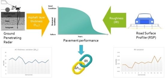
:Pavement condition largely determines its long-term behavior and is of paramount importance for rehabilitation and maintenance management. The use of non-destructive testing (NDT) systems to assess pavement condition has gained much popularity. Often, well-known NDT systems are combined to take full advantage of the capabilities of each system. Combining independent NDT systems to optimize the assessment process is a scientific challenge. With this in mind, the purpose of this paper is to investigate the extent to which data from two independent NDT systems can be combined: pavement thickness obtained with ground penetrating radar (GPR) and roughness data obtained with a road surface profiler (RSP). In particular, the objective of this study is to determine whether the expected variations in asphalt layer thickness, due to the construction process and the different pavement cross sections along the same road/highway road, may have an impact on pavement roughness as expressed in International Roughness Index (IRI) values. GPR and roughness data are collected, processed, and analyzed. The analysis results show that thickness variations are reflected in pavement roughness. The greater the variation in asphalt layer thickness, the greater the IRI values. Furthermore, it is argued that the GPR capabilities can be used for an initial assessment of the expected pavement quality.
1. Introduction
The deterioration rate of asphalt pavements depends on several factors, including not only material properties and pavement design, but also external factors such as the environment and traffic loading. Pavements are designed to withstand the effects of environmental and traffic stresses, and their long-term behavior determines the pavement’s performance. Evaluating pavement condition through monitoring provides valuable information for predicting pavement behavior and thus performance.
Non-destructive testing (NDT) of in-service pavements has become the preferred and most accurate method for evaluating pavement performance. It has the advantage over conventional methods (e.g., core drilling) of not affecting pavement structure and being less time consuming. In addition, most NDT systems allow continuous measurements at steady or high travel speeds.
NDT systems used for pavement evaluation and monitoring include ground penetrating radar (GPR), profilometers, deflectometers, and skid resistance measurement systems. GPR is mainly used for crack detection, determination of pavement layer thickness, and detection of voids and moisture damage [1,2,3]. Deflectometers record the response of the pavement when subjected to an impulse load. Vertical deflections are measured with sensors placed at a specific distance from the center of load and can be used to assess the structural condition of pavements through appropriate processing and analysis. Profilometers are used to determine the roughness, rutting, and texture of pavements.
With the fast development of intelligent transportation systems, multiple sensors including LiDAR and cameras are available on the ground/aerial autonomous vehicles [4,5,6,7] that have the potential to be used to assess the pavement conditions [8]. In a recent study [9], the Unmanned Aerial Vehicle (UAV) was utilized for assessing pavement conditions using the Pavement Condition Index and Surface Distress Index. These methods gain popularity due to the speed of the data acquisition which is one of the major advantages. They are currently capable of capturing various surface defects, such as alligator cracking, bleeding, block cracking, lane/shoulder drop off, longitudinal and transversal cracking, patching, polished aggregate, potholes, rutting, swell, and weathering/raveling, and can at some point replace the traditional visual inspection survey. However, the structural pavement condition and some functional characteristics of the pavement (such as texture and skid resistance) cannot be assessed. Additionally, the data cannot be processed to compute certain pavement evaluation indexes. Therefore, currently these systems can be used as a supportive tool for visual inspection and in conjunction with NDTs for an overall pavement assessment.
The use of GPR has been studied for a variety of pavement surveys, ranging from local pavement deterioration to pavement assessment in a network level [10]. The accuracy of the thickness estimation through GPR has been studied by various researchers [11,12,13]. Depending on the structure of the surveyed pavement, the accuracy of the estimated layer thickness in terms of average absolute error ranges from 2.9 to 7.5%. Apart from thicknesses, air void content can be measured. The basic idea is that the dielectric constant of the asphalt mix is a combination of the dielectric constant of its constitutes and their proportion in the mix. Air void content is directly connected to the compaction. During compaction, the air volume of the asphalt mix is reduced and the volumetrics of the other components of the asphalt mix (asphalt and aggregate) are increased. Since the dielectric value of air (=1.0) is substantially lower than that of either bitumen (≈2.6) or aggregate (≈6.0), as the asphalt is compacted its dielectric value will increase [14]. Another GPR application in flexible pavements is the detection of moisture. The presence of moisture causes easily identified alterations in reflection and transmission patterns [15]. Based on the volumetric mixing model, an expression for calculating the volumetric water content as a function of the porosity, the dielectric constants of air, solid, and water components of the mixture, and the dialectic constant obtained from the electromagnetic measurement is given [16]. The GPR technique has been widely used to detect the location and extent of stripping with varying success [17,18,19]. In most cases, stripping can be seen as an additional positive or negative (reversed reflection polarity) reflection in the pavement [20]. However, similar reflection can be received from an internal asphalt layer with different electrical properties. Due to this fact, reference data such as drill cores and FWD data should always be used to confirm the interpretation [20]. The location of cracks can be determined through the analysis of GPR data, but cracks cannot be further characterized in terms of their length and depth [21].
In recent years, much of the research has focused on the goal of combining NDT systems to derive the maximum benefit from these techniques for pavement evaluation [22,23]. A recent study [24] used GPR in combination with FWD and developed a methodology to determine and quantify the evaluation parameters associated with the deformation data, such as test frequency and acceptance criterion. The importance of determining pavement thickness with GPR was demonstrated in [25] and elsewhere. It was found that the thickness of asphalt pavements estimated with acceptable accuracy using GPR can deviate from the design thickness, which has a great impact on the pavement performance. In addition, a more accurate structural evaluation of the pavement can be achieved by combining FWD (falling weight deflectometer) measurements. In [26], a combined approach of GPR and FWD was used to determine the cause of the observed damage (fatigue cracking and rutting) in a foamed asphalt pavement. Additionally, in [27], the pavement thickness accuracy achieved with GPR allowed the evaluation of a full depth rehabilitation with foamed asphalt (FDR-FA). The combination of GPR and FWD proved to be extremely useful for locating and identifying asphalt delamination and moisture-prone areas [28].
The literature review revealed that the most common practice is to combine GPR with other NDT systems such as FWD to assess the structural condition of the pavement or damage within the pavement structure. However, the main function of pavements is to provide a smooth surface, i.e., a surface with low roughness. Roughness is directly related to ride quality and comfort, but also largely determines pavement life and maintenance costs [29]. Therefore, roughness is one of the different types of deterioration that measure the functional condition of pavements. Roughness can be affected by several parameters, such as road category (urban vs. rural), base type, HMA mix classification, construction and materials quality, age/traffic, and environmental parameters over time. Rural pavements have lower IRI values compared to urban, which can be associated with the fact that rural pavement construction generally has fewer interruptions, resulting in a smoother surface [30]. The HMA mix seems to have an effect on roughness especially in the case of SMA (stone mastic asphalt). SMA mixes are produced with a higher content of coarse aggregate than dense graded mixes, leading to a rough surface [31]. Open graded base courses are associated with higher level of roughness resulting from the absence of fine aggregates that poses a negative effect on workability and compaction [30]. According to [32], the traffic level (accumulated traffic with the passage of time) affects the roughness but does not affect the deterioration rate for a pavement constructed on a good quality subgrade. It was also demonstrated that the roughness deterioration rate under low temperature condition is higher than under medium temperature condition.
For the evaluation of pavement roughness, the International Roughness Index (IRI) is considered a reliable index [33]. The IRI is a measure for roughness based on the response of a generic motor vehicle to roughness of the road surface. Essentially, it describes the mounting and dropping of a lateral profile of the total investigated length. Therefore, it is determined based on the geometric characteristics of the road surface. Various measurement systems are available for the recording and measurement of IRI. According to [34], they are categorized into four levels depending on their accuracy. The most accurate are those that record the pavement surface profile and convert it to an IRI value. Systems that fall into this category are laser profilers, dipstick, walking profiler, profilometers, and inertial profilers.
The recording and evaluation of the IRI index has two objectives: acceptance of a new pavement as part of quality control and monitoring of the functional condition of the pavement during its service life in order to plan necessary maintenance measures.
However, as mentioned earlier, pavement thickness plays an important role in pavement quality and performance. Given the importance of evaluating pavement roughness on the one hand and the dependence of pavement performance on pavement thickness on the other, the question arises whether profilometer and GPR data can be combined to provide more comprehensive information on pavement quality. So far, not much attention has been paid to this research area, and there are only a few studies that address the relationship between IRI and pavement thickness. According to the analysis results of [30], the initial roughness of asphalt pavements is highly dependent on asphalt layer thickness. An increase in asphalt layer thickness leads to a decrease in IRI. This is consistent with another study [32], which investigated the factors affecting pavement roughness. Pavement thickness was calculated as the sum of the equivalent asphalt layer thickness for each layer of the pavement structure. Various conditions such as precipitation, temperature, traffic, and subgrade were considered. In almost all cases, the increase in pavement thickness had a noticeable effect on pavement roughness, in the sense that the thicker the pavement, the lower the IRI value. In a recent study, the factors contributing to pavement performance were investigated using different approaches to analyze Long-Term Pavement Performance Program (LTPP) data [35]. One of the main findings was that asphalt layer thickness is a statistically significant parameter affecting pavement roughness. In particular, the mean IRI value decreases with increasing asphalt layer thickness. A recent study [36] investigated the combined use of FWD, GPR, and profilometers to evaluate pavement roughness. GPR thickness data were used along with deflection data from FWD as input for estimating the structural condition of the pavement. The analysis of the integration of GPR, FWD, and profilometer data clearly showed that there is a relationship between the condition of the subgrade and the pavement quality.
All the afore-mentioned studies recognize that pavement has the most noticeable effect on roughness.
With this in mind, this study addresses the integration of GPR thickness data with roughness data to better assess pavement quality and performance. Along a highway section, the thickness of the asphalt layers varies due to the different pavement cross sections resulting from the pavement design. However, variations also occur within the same cross section mainly due to the construction process and poor-quality control procedures. The asphalt mixture construction depends on a variety of factors, including environmental conditions, characteristics of the mixture, and operating systems parameters (i.e., type of compaction system). In other words, the thickness of asphalt layers in paved condition can be expected to vary around the target thickness (design thickness) of a road section. Similar research has shown that there is a large variation in thickness between the designed thickness and the actual paved thickness [37,38]. These variations follow a normal distribution [39,40,41]. On the other hand, thickness variation along a road section appears due to alternative pavement cross sections. These variations are random.
Based on the above, this study aims to extend the results of previous studies by focusing on the effects of thickness variation (instead of absolute thickness) on pavement ride quality, expressed in IRI values. Thickness variations resulting either from expected variations between the design and paved condition or from the transition from one cross section to another along the same highway road were considered. Investigating the effects of thickness variation on pavement performance (in terms of ride quality) enables the assessment of performance models and equations.
2. Materials and Methods
2.1. Test Sections
To achieve the objective of the present study, a road test was conducted. Specifically, NDT measurements were made along two highway flexible pavement sections (A and B). The total length was 60 km. Both cross sections consist of the asphalt layers, the base, the subbase, and the subgrade. Asphalt layers consist of the wearing course and the asphalt base layer. The wearing course is a semi open graded mixture with 80–100 asphalt penetration modified with SBS 4% and limestone and steel slag aggregate. The asphalt base layer mixture is dense graded and was produced using 50–70 grade asphalt penetration and limestone aggregates. The base and subbase courses are dense graded and consist of unbound aggregates. The subgrade support is considered good (CBR > 20%). Each highway section was further divided in subsections with the same thickness design. The asphalt layers design thicknesses are given in Table 1. The climatic conditions prevailing in regions of the two highways do not show significant differences (Mediterranean climate). Highway sections A and B are part of a periodical monitoring system and as such a data base of the pavements characteristics is available and is updated with a new set of collected data on an annual basis. Roughness measurements are realized once in a year during the same period of the year. Therefore, in order to eliminate the effect of traffic in the analysis, the roughness data were retrieved from the database so that traffic (accumulated annual average daily traffic) was on approximately the same level for all sections.
Given that the parameters of materials, the traffic, and the climatic conditions are more or less common in all sections, the analysis will include only the effect of asphalt mix thickness variation in roughness index IRI.
For the measurements, a GPR system was used to determine the asphalt layer thickness and an inertial profiler called Road Surface Profilometer-RSP was used to determine the IRI index.
2.2. GPR Survey
In order to record the pavement stratigraphy and determine the layer thicknesses, an air-coupled GPR system was used with an antenna of 1000 MHz frequency Type 4108 Horn [42]. The fundamental operating principle of the system is based on the electromagnetic theory, since the signals that are emitted are electromagnetic waves that can be mathematically described by the equations of electromagnetic theory (Maxwell). The GPR system is positioned close to the under-investigation surface, so that the waves are directed to it. When they encounter material with different electromagnetic properties (in this case different pavement layers), on the one hand part of them is reflected back to the receiver and on the other hand the propagation velocity changes. Principally, the GPR system measures the two-way travel time of emitted and reflected EM wave. Based on this time and the properties of the materials, the thicknesses of the individual layers of the pavement are calculated.
Figure 1 presents an example of the amplitudes and time intervals observed in case of a flexible pavement. The key component with a direct effect on the wave velocity is the dielectric constant of the materials. Pavement layers constitute of different materials and as such each layer has a different dielectric constant. The relationship between dielectric constant and velocity is inversely proportional. Thus, the higher the dielectric constant, the lower the electromagnetic wave velocity. Dielectric constant of the various pavement layers can be calculated considering the peak amplitudes (A0, A1, …, Ai) of the interfaces and the amplitude of the incident GPR signal [43]. For the determination of the incident GPR signal, a perfect electromagnetic reflector (copper plate) is used (Figure 2).
The basic apparatus of a GPR system is the following:
2.3. RSP Survey
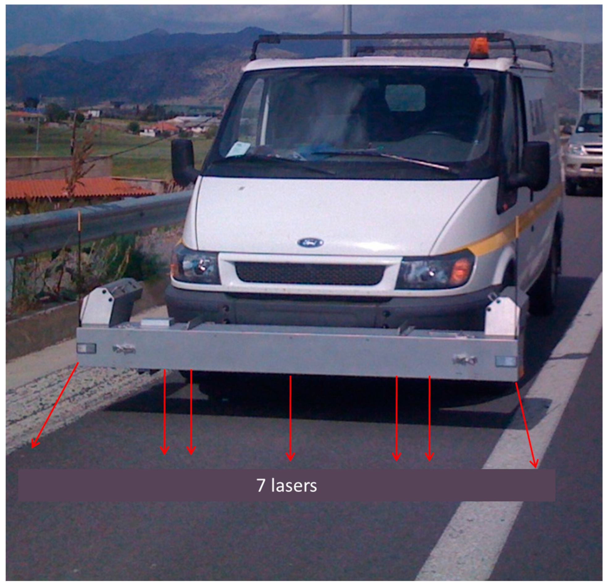
RSP is an inertial profiler that uses a combination of laser and accelerometer to measure the longitudinal elevation profile of the road for high degree accuracy at highway speeds [46]. Its basic unit is a rigid beam of 3.2 m length, where seven lasers and two accelerometers are embedded. The beam is adapted to the front of a properly configured vehicle (Figure 3). RSP records the following parameters every 25 mm during the vehicle movement:
- The vertical displacement of the beam from the road surface.
- The vertical acceleration of the beam.
- The time and distance that the two aforementioned parameters are recorded.
The profile is then analyzed to calculate IRI values for road surface. It is calculated using a quarter-car vehicle math model, whose response is accumulated to yield a roughness index with units of slope (m/km). The quarter-car model is a theoretical system that consists of the vehicle wheel, the mass of the vehicle that corresponds to a single wheel, of the suspension–damping system, and of the mass of the axle–wheel–tire system (Figure 4).
Specifically, the quarter-car model used for the calculation of IRI index consist of the following:
- The sprung mass—ms (kg), which is the mass of the part of the vehicle that burdens the suspension and includes a percent of the weight of the suspension.
- The unsprung mass—mu (kg), which is the mass corresponding to the weight that does not burden the suspension system but is supported by the wheel or the tire and follows its displacements.
- The suspension spring with coefficient ks (kN/m).
- The suspension damping coefficient (cs) (kN s/m).
- The tire spring rate (kt) (kN/m).
For the calculation of the IRI index, the values of the aforementioned parameters need to be determined. The set of values as described in [47] that are used for the calculation of the IRI, through appropriate algorithm, constitute the “golden car”. In other words, it is the quarter car with specific values of the parameters. The principal idea for the IRI calculation is to model the movement of the quarter car on the pavement surface and the calculation of the total displacement of the suspension. IRI values equal to zero correspond to a totally smooth pavement, while IRI values around ten (10 m/km) indicate a practically impassable road surface [48].
Profile elevations were measured in both wheel paths simultaneously. For the analysis, the average value of the IRI in the wheel paths was considered. The data collection field program [49] gives step-by-step guide for the calibration of lasers, accelerometers, and distance measuring instrument (DMI), making calibration simple and easy to perform.
2.4. Data Processing
There are various studies dealing with the methodology followed for the analysis of the GPR data [21]. The determination of the thickness through the time interval between the reflected pulses from different layers and the dielectric properties of the layer was found to have an average error of about 5% when the core thickness was paralleled the corresponding data recorded by the GPR system [50]. The use of multi-offset array test (MOA) procedure resulted in low accuracy of the estimated thicknesses [51]. In the same study, the reflection amplitude coefficient methodology (RAC) procedure produced errors ranging from 5 to 9% with a tendency to increase for larger depths [51]. In another study [52], the common mid-point approach (CMP) was investigated for its accuracy in estimating the pavement thickness. For this purpose, two sets of antennas were used (air-coupled). Furthermore, the results of the CMP approach were compared to the ones of the surface reflection method (SRM). It was concluded that the CMP approach leads to more accurate results for asphalt layers of about 6 cm, since the average error was about 6% compared to 18% for the SRM. For asphalt layer thicknesses up to 13 cm, errors from both approached reached 7%. An extended CMP method was developed by using two air-coupled GPR systems [53]. The prediction error of the asphalt thickness ranged from 2 to 23%. Higher error was observed in the case of asphalt layer thickness up to 6.3 cm, while for larger thicknesses, the error decreased. Other procedures studied involve the use of a multi-offset array [54], image processing algorithms [53], and truncation algorithm [55].
In light of the above, it is evident that a lot of approaches have been developed for the analysis of GPR data in an effort to minimize the errors in the estimation of pavement thicknesses. In most of the cases, the minimum error achieved was around 5%. In this study, the thickness determination was achieved by combining the time interval and the dielectric constant calibrated with core data, as presented in [50], due to the simplicity of the method and the low average error.
GPR data processing and analysis was performed using appropriate software [56]. The GPR analysis consists of the following steps: preprocessing, processing, and interpretation.
In the preprocessing phase, GPR data are edited in such a way that the raw data itself will not be changed. In this phase, the GPR editing features normally used are file reversal, cutting and combining, scaling, and linking data to GPS coordinates or to different road address data bases [56]. During preprocessing, it must be ensured that GPR signal polarity and color scales follow certain rules. In a measured pulse from a metal plate in a single scan mode, the maximum peak should always point to the right, and it should be referred to as the positive reflection, and in a line scan format using a grey scale, it should be white. The two smaller peaks around the positive peaks are called negative peaks, and in a line scan format using a grey scale, they should be black [57].
In the processing phase, signals from raw pavement data, end reflection, and metal reflection are elaborated [57]. The end reflection is a pulse, which is removed from the actual road measurement data, so one could check that the gain and the data format correspond with those of the road measurement. It is only necessary to do this if the direct wave has clutter below the pavement surface level. The template pulse is needed to improve the vertical resolution in the upper part of the GPR data (pavement bottom), as well as for calculating the dielectric value of the pavement.
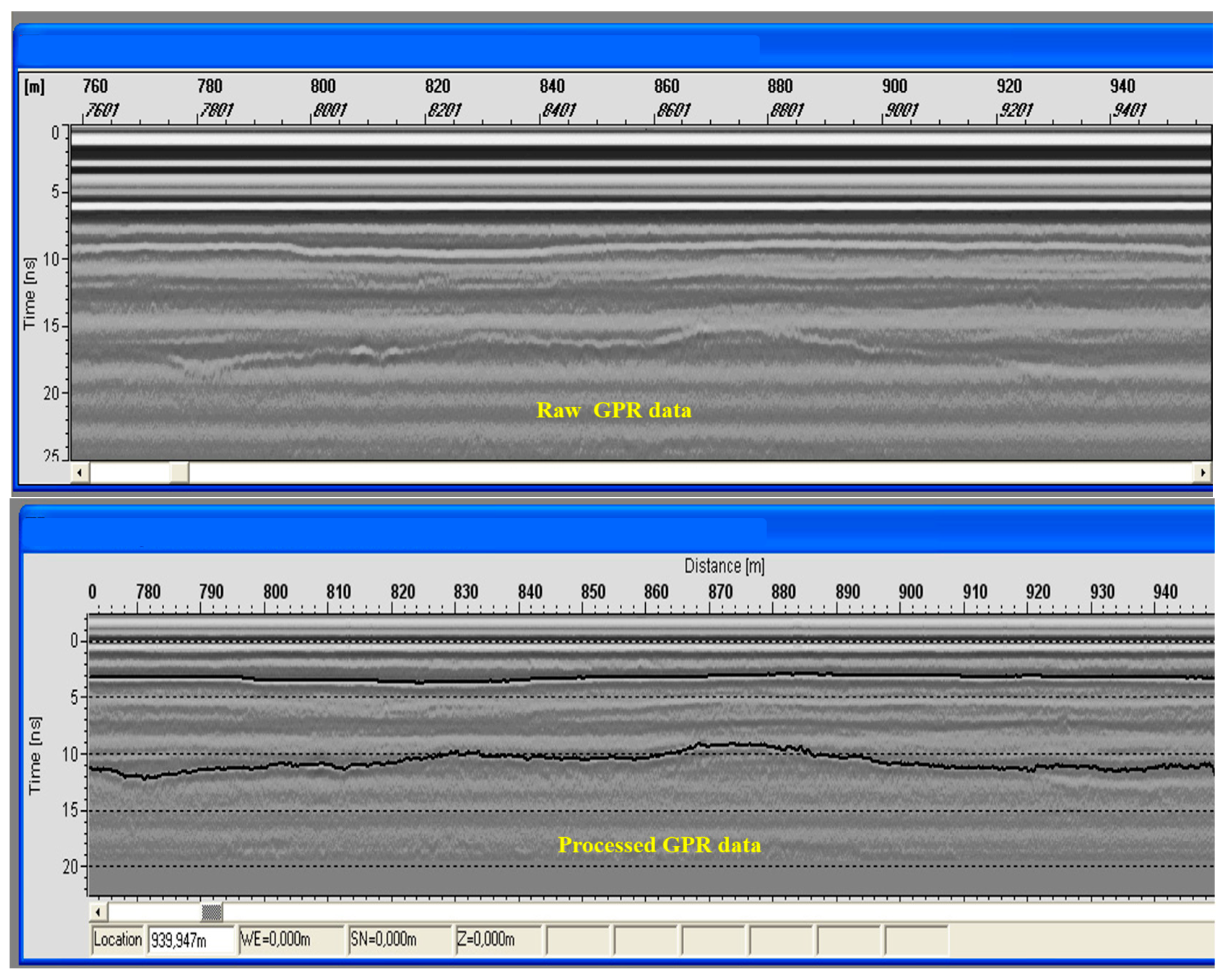
During the processing phase, data filtering must be also performed. Different filter settings can be tested in order to see if they improve the data quality. After the metal plate calibration and template subtraction, other filters can be used. A special “background removal” filter has also been proven to improve the data quality. In Figure 5, raw data as well as data after processing are presented.
GPR data analysis in the case of pavements is a complex procedure, due to the fact that it consists of different layers with non-homogenous materials. For the determination of their dielectric constant, the use of relevant bibliography is not recommended. In order to accomplish the maximum possible accuracy in estimating the thicknesses, limited core sampling was performed in all subsections. This way, it was possible to calculate the parameters that are needed for converting time to thickness.
The thickness of a pavement layer using GPR can be determined by recording the time difference between the reflected pulses from different layers and the dielectric properties of the surveyed layer. The thickness of the nth layer could be computed according to the following equation [43]:
where dn is the thickness of the nth layer, tn is the electromagnetic (EM) two-way travel time through the nth layer as shown in Figure 1, c is the speed of light free space (≈3 × 10⁸ m/s), and εr,n is the dielectric constant of the nth layer. In order for the layer thickness to be estimated based on the above-mentioned equation, the knowledge of the dielectric properties of layer materials is necessary.
Table 2 presents the estimated through the GPR measurements asphalt layer average thickness per subsection and the standard deviation. Thickness data were exported at an interval of 10 m.
The average as built thicknesses are close to the design thicknesses in each subsection and the standard deviation is low for most of the cases.
RSP measurements were continuous, and IRI data were exported at 10 m intervals. The data were recorded continuously and were exported at 10 m intervals. For the analysis, the AC thickness difference in segments of 100 m was calculated (i.e., ΔhAC = hAC at position 100 m-hAC at position 200 m). The IRI average value (IRIav) was calculated for the same 100 m segments.
3. Results
Figure 6 presents an overall of the data used for the analysis. X axis is the number of the 100 m segments (600 segments in a total length of 60 km). Differences in hAC within the segments vary from 0 to 9 cm, while IRIav values range between 0.16 and 2.65. It is noted that in most cases, differences in hAC greater than 6 cm are due to the transaction from one subsection to another along the same highway section (i.e., the transaction from A1 to A2).
From a first glance, it is not evident whether the IRI values can be correlated with the thickness difference of the asphalt layers. However, a trend is scarcely noticeable in which IRIav values seem to be higher at higher ΔhAC values.
Further analysis was conducted in which the ΔhAC values were grouped in three categories:
- 0 ≤ ΔhAC ≤ 2 cm
- 2 < ΔhAC ≤ 5 cm
- ΔhAC > 5 cm
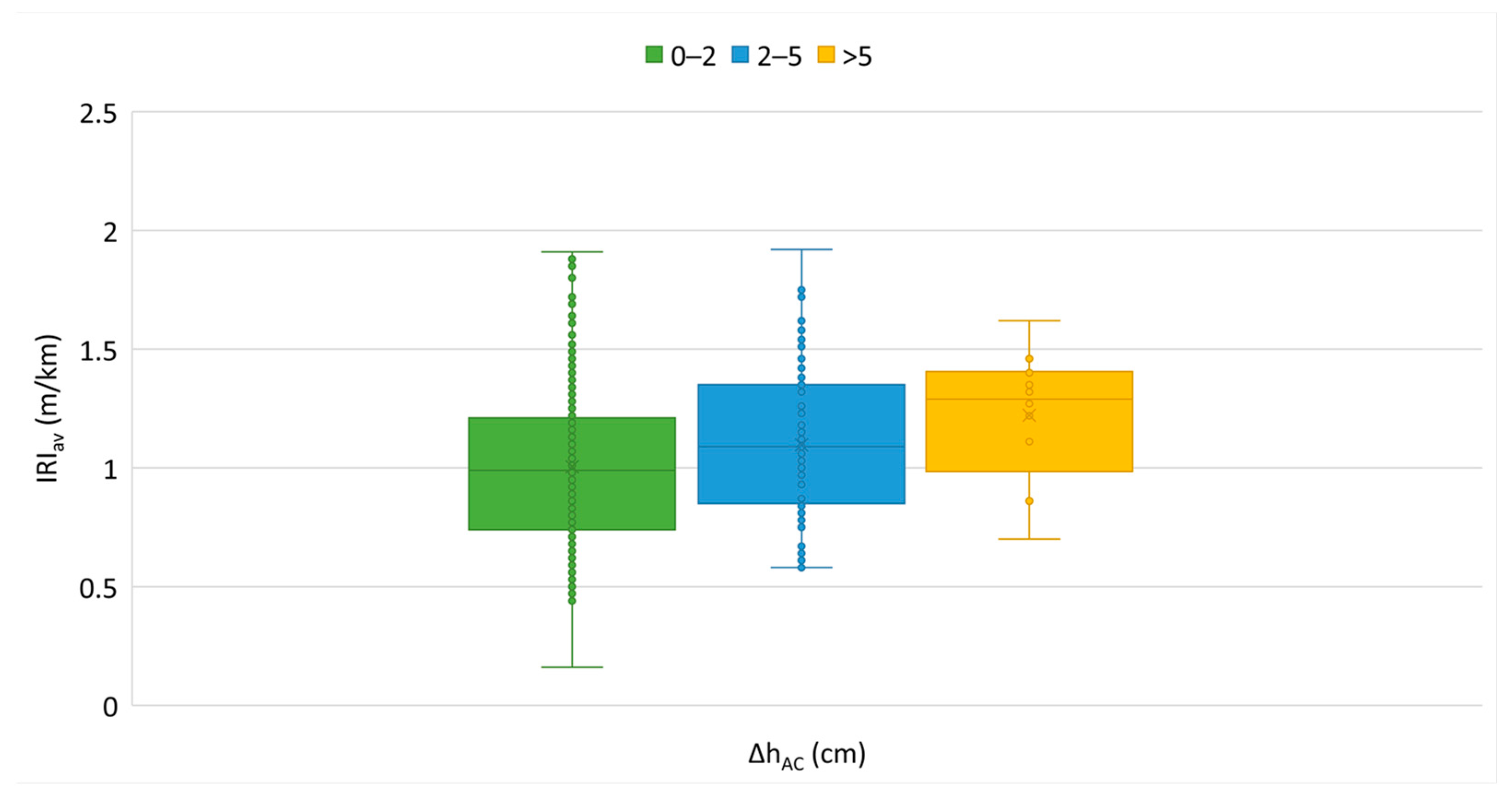
The IRIav values that fall in each one of these ΔhAC categories are presented in Figure 7 in the form of boxplots.
The boxplot is an efficient way of displaying five numerical data of a series of observations: of the smallest observation of the first quartile (Q1), the median of the third quartile (Q3), and the greatest observation. The distances between the different parts of the boxplot are indicative of the dispersion and asymmetry of the data.
The focal observation from Figure 7 is that there is the tendency for higher IRIav values with the increase in ΔhAC values. Table 3 contains the descriptive statistics of the IRIav values for the three ΔhAC categories.
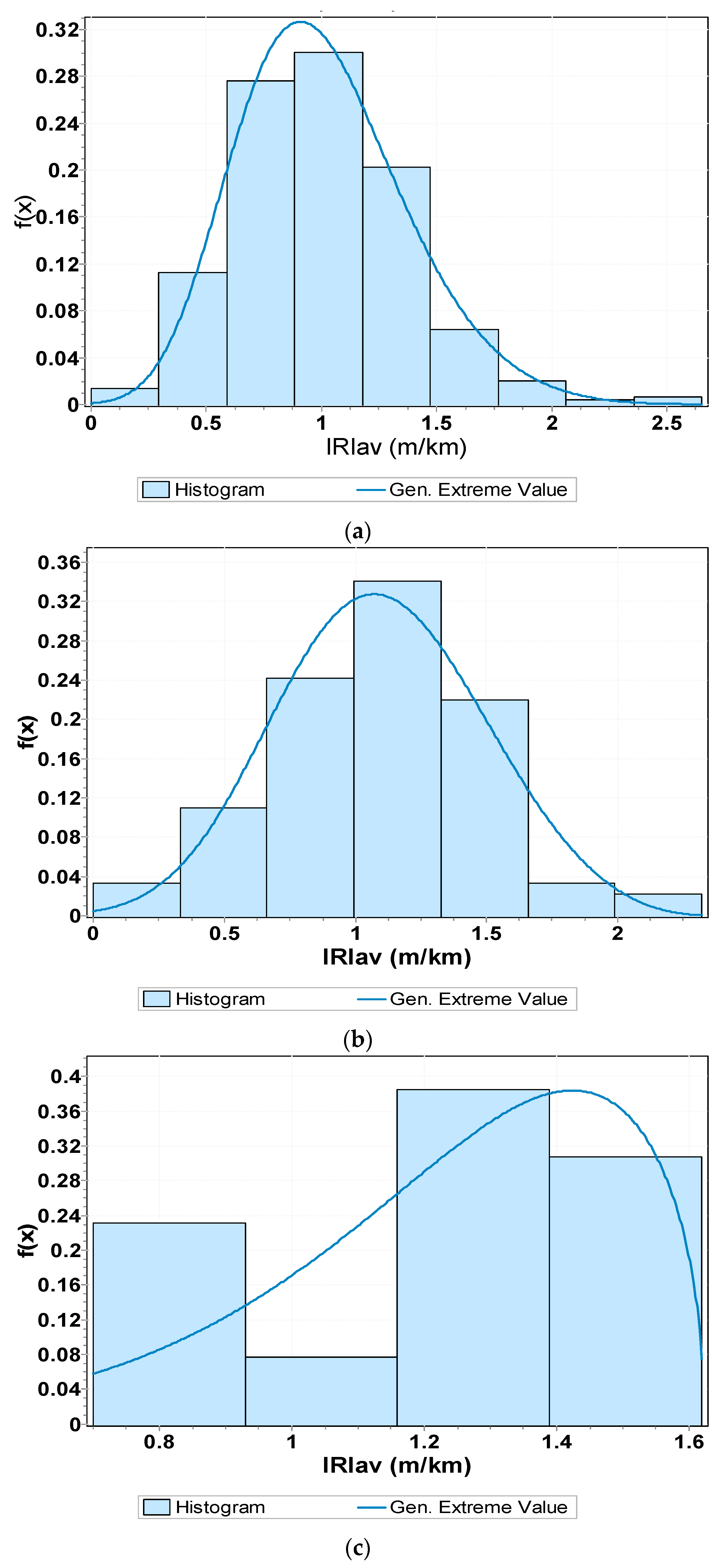
The high value of the coefficient of variance (>0.10) indicates that there is a large variation in IRIav values. This is expected since IRI values grouped in these categories do not represent the smoothness of a single pavement section, but rather IRI data from all sections and subsections. Thus, the riding quality cannot be represented by the mean value. On these grounds, it was investigated whether a distribution can be applied in order to describe the data. The generalized extreme value (Gen. Extreme) distribution was examined. This distribution is a model that combines the Gumbel, Frechet, and Weibull distributions [58]. The parameters of the density probability function are z = (x − μ)/σ, σ and k, where μ is the location parameter, σ is the scale parameter (σ > 0), and k is the shape parameter. Depending on the k value, we can have each of the following distributions:
- k = 0 Gumbel Distribution
- k > 0 Frechet Distribution
- k < 0 Weibull Distribution
Figure 8 describes the distribution of the IRIav values. The parameters of the generalized extreme value distribution are presented in Table 2. For the goodness of fit, the Kolmogorov–Smirnov test was applied, and the results (test statistic along with significance level) are shown in Table 4. The location parameter μ is considered representative of the samples since it is the value with the maximum probability of occurrence.
Based on parameter μ value, the tendency for higher IRIav values with the increase in ΔhAC values becomes more evident and justified. To thoroughly elaborate the analysis results, the μ values are used to demonstrate the roughness level as well as the percentage difference of IRI values with asphalt layers thickness variation (Figure 9).
Figure 9 indicates that higher AC thickness variations (>5 cm) result in a greater percentage increase of IRI. It should be noted, however, that the cases in which the thickness varies by more than 5 cm correspond to the change in the pavement cross section along the same highway.
4. Discussion
The evaluation of the structural and functional condition of pavements requires the use of different NDT systems that operate according to different principles. Each of these systems provides specific data on its own, which limits their capabilities. The combination of NDT systems and the integrated analysis of their data can overcome these limitations and provide a more comprehensive pavement assessment.
In this study, the possible relationship between asphalt layer thickness variation and pavement roughness was investigated. GPR and profilometer measurements were performed in sections of two different highways. The analytical results presented in this paper show that the pavement performance in terms of pavement roughness is related to the variation of asphalt layer thickness. In particular, this study proves that it is useful to investigate the effects of asphalt layer thickness on roughness in addition to other studies, since the IRI values seem to be affected by the variation of asphalt layer thickness. The more the layer thickness varies, the lower the ride quality of the pavement surface.
Specifically, the variation in asphalt layer thickness was divided into three categories to investigate whether the effects on IRI remained constant. The IRI values in each of the three categories can be described by the generalized extreme value (Gen. Extreme) distribution. Based on the characteristic value, it can be concluded that asphalt layer thickness variations greater than 5 cm result in a larger percentage increase in IRI. In other words, it is proved that pavement sections with a high degree of asphalt layer thickness inhomogeneity tend to have poorer ride quality.
Consistent with the above, it is argued that GPR capabilities can be extended beyond pavement thickness determination and structural evaluation to an initial assessment of expected pavement ride quality (when surface elevation is considered).
5. Conclusions
In this research study, an approach was developed in which in situ collected pavement data (pavement profile and stratigraphy) were analyzed together to demonstrate a favorable quality control framework for identifying areas that may exhibit more rapid deterioration in ride quality during pavement operation. Variation in asphalt layer thickness was shown to affect pavement roughness. It was shown that, for a given pavement cross section, the layer thicknesses accumulate around the design value during the construction phase, especially during paving and compaction of the asphalt mix. In this study, it was demonstrated that these variations are reflected in the roughness of the pavement. Moreover, it is proved that the transition from a pavement cross section to another along the same road/highway section affects ride quality due to the thickness variations. In general, it can be stated that the more the thickness of the asphalt layer varies, the higher the IRI values.
Because roughness is an extremely important indicator of pavement performance that directly affects road user safety, areas with elevated IRI values should be monitored as part of a pavement monitoring system to determine rehabilitation actions in a timely manner. In this sense, the relationship between IRI and thickness change can be considered a useful tool for planning maintenance systems.
Overall, the approach developed is considered a robust method that optimizes the required testing. Further investigation is needed, and more pavement sections should be considered to support the numerical results. In addition, it should be investigated whether the variation of the base/subbase course thickness has an influence on the pavement roughness. The results could be further validated with a more systematic approach that considers a broader range of roads in terms of base type, asphalt mix classification, construction and material quality, age/traffic, and environmental parameters. In addition, various approaches to GPR data processing could be applied, including methods to handle in situ noise and mechanical vibration of the GPR antennas during high-speed measurements.
Author Contributions
Conceptualization C.P., K.G. and A.L.; methodology, C.P.; analysis, K.G.; writing—original draft preparation, K.G.; writing—review and editing, C.P. and A.L. All authors have read and agreed to the published version of the manuscript.
Funding
This research received no external funding.
Data Availability Statement
Not applicable.
Conflicts of Interest
The authors declare no conflict of interest.
References
- Plati, C.; Loizos, A.; Gkyrtis, K. Assessment of Modern Roadways Using Non-destructive Geophysical Surveying Techniques. Surv. Geophys. 2020, 41, 395–430. [Google Scholar] [CrossRef]
- Benedetto, A.; Tosti, F.; Ortuani, B.; Giudici, M.; Mele, M. Mapping the spatial variation of soil moisture at the large scale using GPR for pavement applications. Near Surf. Geophys. 2015, 13, 269–278. [Google Scholar] [CrossRef]
- Benedetto, A.; Tosti, F.; Bianchini Ciampoli, L.; D’Amico, F. An overview of ground-penetrating radar signal processing techniques for road inspections. Signal Process. 2017, 132, 201–209. [Google Scholar] [CrossRef]
- Xia, X.; Meng, Z.; Han, X.; Li, H.; Tsukiji, T.; Xu, R.; Zheng, Z.; Ma, J. An automated driving systems data acquisition and analytics platform. Transp. Res. Part C 2023, 151, 104–120. [Google Scholar] [CrossRef]
- Liu, W.; Quijano, K.; Crawford, M.M. YOLOv5-Tassel: Detecting Tassels in RGB UAV Imagery with Improved YOLOv5 Based on Transfer Learning. IEEE J. Sel. Top. Appl. Earth Obs. Remote Sens. 2022, 15, 8085–8094. [Google Scholar] [CrossRef]
- Xia, X.; Hashemi, E.; Xiong, L.; Khajepour, A. Autonomous Vehicle Kinematics and Dynamics Synthesis for Sideslip Angle Estimation Based on Consensus Kalman Filter. IEEE Trans. Control. Syst. Technol. 2023, 31, 179–192. [Google Scholar] [CrossRef]
- Gao, L.; Xiong, L.; Xia, X.; Lu, Y.; Yu, Z.; Khajepour, A. Improved Vehicle Localization Using On-Board Sensors and Vehicle Lateral Velocity. IEEE Sens. J. 2022, 22, 6818–6831. [Google Scholar] [CrossRef]
- Ravi, R.; Habib, A.; Bullock, D. Pothole Mapping and Patching Quantity Estimates using LiDAR-Based Mobile Mapping Systems. Transp. Res. Rec. 2020, 2674, 124–134. [Google Scholar] [CrossRef]
- Astor, Y.; Nabesima, Y.; Utami, R.; Sihombing, A.V.R.; Adli, M.; Firdaus, M.R. Unmanned aerial vehicle implementation for pavement condition survey. Transp. Eng. 2023, 12, 100168. [Google Scholar] [CrossRef]
- Maser, K.R. Condition Assessment of Transportation Infrastructure Using Ground Penetrating Radar. J. Infrastruct. Syst. 1996, 2, 94–101. [Google Scholar] [CrossRef]
- Lahouar, S.; Al-Qadi, I.L.; Loulizi, A.; Clark, T.M.; Lee, D.T. Approach to Determining In Situ Dielectric Constant of Pavements: Development and Implementation at Interstate 81 in Virginia. In Transportation Research Record: Journal of the Transportation Research Board; No. 1806; Transportation Research Board of the National Academies: Washington, DC, USA, 2002; pp. 81–87. [Google Scholar]
- Al-Qadi, I.L.; Lahouar, S.; Loulizi, A. Successful Application of Ground-Penetrating Radar for Quality Assurance—Quality Control of New Pavements. In Transportation Research Record: Journal of the Transportation Research Board; No. 1861; Transportation Research Board of the National Academies: Washington, DC, USA, 2003; pp. 86–97. [Google Scholar]
- Maser, K.R.; Scullion, T. Automated Pavement Subsurface Profiling Using Radar: Case Studies of Four Experimental Field Sites. In Transportation Research Record: Journal of the Transportation Research Board; No. 1344; Transportation Research Board of the National Academies: Washington, DC, USA, 1992; pp. 148–154. [Google Scholar]
- Loken, M. Current State of the Art and Practise of Using GPR for Minnesota Roadway Applications; Minnesota Local Research Board; Office of Research Activities: St. Louis, MN, USA, 2005. [Google Scholar]
- Grote, K.; Hubbard, S.; Harvey, J.; Rubin, Y. Evaluation of Infiltration in Layered Pavements Using Surface GPR Reflection Techniques. J. Appl. Geophys. 2005, 57, 129–153. [Google Scholar] [CrossRef]
- Roth, K.; Schulin, R.; Fluhler, H.; Attinger, W. Calibration of Time Domain Reflectometry for Water Content Measurements Using Composite Dielectric Approach. Water Resour. Res. 1990, 26, 2267–2273. [Google Scholar] [CrossRef]
- Rmelie; Scullion, T. Detecting Stripping in Asphalt Concrete Layers Using Ground Penetrating Radar. In Transportation Research Record: Journal of the Transportation Research Board; No 1568; Transportation Research Board of the National Academies: Washington, DC, USA, 1997; pp. 165–174. [Google Scholar]
- Hammons, M.I.; Von Quintus, H.; Geary, G.M.; Wu, P.Y.; Jared, D.M. Detection of Stripping in Hot-Mix Asphalt. In Transportation Research Record: Journal of the Transportation Research Board; No. 1949; Transportation Research Board of the National Academies: Washington, DC, USA, 2006; pp. 20–31. [Google Scholar]
- Scullion, T.; Rmeili, E.H. Detection of Stripping in Asphalt Concrete Layers Using Ground Penetrating Radar; Research report 2964-S; Texas Transportation Institute: College Station, TX, USA, 1997.
- Saarenketo, T.; Scullion, T. Road Evaluation with Ground Penetrating Radar. J. Appl. Geophys. 2000, 43, 119–138. [Google Scholar] [CrossRef]
- Ahmad, N.; Lorenzl, H.; Wistuba, M.P. Crack detection in asphalt pavements—How useful is the GPR? In Proceedings of the 6th International Workshop on Advanced Ground Penetrating Radar (IWAGPR), Aachen, Germany, 22–24 June 2011; pp. 1–6. [Google Scholar]
- Tosti, F.; Bianchini Ciampoli, L.; D’Amico, F.; Alani, A.M.; Benedetto, A. An experimental-based model for the assessment of the mechanical properties of road pavements using ground-penetrating radar. Constr. Build. Mater. 2018, 165, 966–974. [Google Scholar] [CrossRef]
- Elseicy, A.; Alonso-Díaz, A.; Solla, M.; Rasol, M.; Santos-Assunçao, S. Combined Use of GPR and Other NDTs for Road Pavement Assessment: An Overview. Remote. Sens. 2022, 14, 4336. [Google Scholar] [CrossRef]
- Xiong, C.; Yu, J.; Zhang, X. Use of NDT systems to investigate pavement reconstruction needs and improve maintenance treatment decision-making. Int. J. Pavement Eng. 2021, 1–15. [Google Scholar] [CrossRef]
- Marecos, V.; Fontul, S.; de Lurdes Antunes, M.; Solla, M. Evaluation of a highway pavement using non-destructive tests: Falling Weight Deflectometer and Ground Penetrating Radar. Constr. Build. Mater. 2017, 154, 1164–1172. [Google Scholar] [CrossRef]
- Chen, D.-H.; Bilyeu, J.; Scullion, T.; Nazarian, N.; Chiu, C.-T. Failure Investigation of a Foamed-Asphalt Highway Project. J. Infrastruct. Syst. 2006, 12, 33–40. [Google Scholar] [CrossRef]
- Plati, C.; Georgouli, K.; Cliatt, B.; Loizos, A. Incorporation of GPR data into genetic algorithms for assessing recycled pavements. Constr. Build. Mater. 2017, 154, 1263–1271. [Google Scholar] [CrossRef]
- Chen, D.H.; Scullion, T. Forensic Investigations of Roadway Pavement Failures. J. Perform. Constr. Facil. 2008, 22, 35–44. [Google Scholar] [CrossRef] [Green Version]
- Hong-hai, L.; Zhong-xin, X.; Zhi-geng, Z.; Bing, L. Research and verification of transfer model for roughness conditions of pavement constructio. Int. J. Pavement Res. Technol. 2016, 9, 222–227. [Google Scholar] [CrossRef] [Green Version]
- Wen, H. Design Factors Affecting the Initial Roughness of Asphalt Pavements. Int. J. Pavement Res. Technol. 2011, 4, 268–273. [Google Scholar]
- Yero, S.A.; Hainin, M.R.; Yaacob, H. Determination of Surface Roughness Index of Various Bituminous Pavements. Int. J. Res. Rev. Appl. Sci. 2012, 13, 98–103. [Google Scholar]
- Elbheiry, M.; Kandil, K.; Kotb, A. Investigation of Factors Affecting Pavement Roughness. Eng. Res. J. 2011, 132, 1–13. [Google Scholar]
- Sun, X.; Wang, H.; Mei, S. Highway performance prediction model of International Roughness Index based on panel data analysis in subtropical monsoon climate. Constr. Build. Mater. 2023, 366, 130232. [Google Scholar] [CrossRef]
- Wang, G.; Burrow, M.; Ghataora, G. Study of the Factors Affecting Road Roughness Measurement Using Smartphones. J. Infrastruct. Syst. 2020, 26, 4020020. [Google Scholar] [CrossRef]
- Bhandari, S.; Luo, X.; Wang, F. Understanding the effects of structural factors and traffic loading on flexible pavement performance. Int. J. Pavement Res. Technol. 2022, 12, 258–272. [Google Scholar] [CrossRef]
- Gkyrtis, K.; Loizos, A.; Plati, C. Integrating Pavement Sensing Data for Pavement Condition Evaluation. Sensors 2021, 21, 3104. [Google Scholar] [CrossRef]
- Mladenovic, G.; Jiang, Y.J.; Selezneva, O.; Aref, S.; Darter, M. Comparison of As-Constructed and As-Designed Flexible Pavement Layer Thicknesses. In Transportation Research Record: Journal of the Transportation Research Board; Transportation Research Board of the National Academies: Washington, DC, USA, 2003; Volume 1853, pp. 165–176. [Google Scholar]
- Xu, T.; Huang, X. Investigation into causes of in-place rutting in asphalt pavement. Constr. Build. Mater. 2012, 28, 525–530. [Google Scholar] [CrossRef]
- Timm, D.H.; Newcomb, D.E.; Galambos, T.V. Incorporation of reliability into mechanistic-empirical pavement design. Transp. Res. Rec. J. Transp. Res. Board 2000, 1730, 73–80. [Google Scholar] [CrossRef]
- Noureldin, A.; Sharaf, E.; Arafah, A.; Al-Sugair, F. Estimation of standard deviation of predicted performance of flexible pavements using AASHTO Model. Transp. Res. Rec. 1994, 1449, 46–56. [Google Scholar]
- Aguiar-Moya, J.P.; Banerjee, A.; Prozzi, J.A. Sensitivity analysis of the M-E PDG using measured probability distributions of pavement layer thickness. In Proceedings of the 88th Transportation Research Board Annual Meeting, Washington, DC, USA, 11–15 January 2009. Paper no. 09-0412. [Google Scholar]
- Geophysical Survey Sytems Inc. Model 4108 Horn Antenna. In System Settings and User Notes; Geophysical Survey Sytems Inc.: Nashua, NH, USA, 2002. [Google Scholar]
- Al-Qadi, I.L.; Lahouar, S. Measuring Layer Thicknesses with GPR—Theory to Practice. Constr. Build. Mater. 2005, 19, 763–772. [Google Scholar] [CrossRef]
- Geophysical Survey Sytems Inc. Radan for Windows. User’s Manual, Geophysical Survey Systems INC (GSSI); Geophysical Survey Sytems Inc.: Nashua, NH, USA, 2002. [Google Scholar]
- Roadscanners. Road Doctor Software, User’s Guide, Version 1.1; Roadscanners: Rovaniemi, Finland, 2001.
- Dynatest. Dynatest 5051 Mark III/IV, Road Surface Profiler, Test Systems. Owner’s Manual, Version 2.3.4; Dynatest: Søborg, Denmark, 2007.
- Sayers, M.W.; Karamihas, S.M. The Little Book of Profiling: Basic Information about Measuring and Interpreting Road Profiles; Transportation Research Institute: Ann Arbor, MI, USA, 1998. [Google Scholar]
- ASTM. E 1926–98; Standard Practice for Computing International Roughness Index of Roads from Longitudinal Profile Measurements. American Society for Testing and Materials: West Conshohocken, PA, USA, 2021.
- Dynatest. Dynatest Data Collection (DDC); Dynatest: Søborg, Denmark, 2007. [Google Scholar]
- Wang, L.; Gu, X.; Liu, Z.; Wu, W.; Wang, D. Automatic detection of asphalt pavement thickness: A method combining GPR images and improved Canny algorithm. Measurement 2022, 196, 111248. [Google Scholar] [CrossRef]
- Loizos, A.; Plati, C. Accuracy of pavement thicknesses estimation using different ground penetrating radar analysis approaches. NDT E Int. 2007, 40, 147–157. [Google Scholar] [CrossRef]
- Liuzzo-Scorpo, A.; Cook, A. Accuracy evaluation of traffic-speed coreless GPR techniques in pavement layer thickness estimation. In Proceedings of the 9th International Workshop on Advanced Ground Penetrating Radar (IWAGPR), Edinburgh, UK, 28–30 June 2017; pp. 1–6. [Google Scholar] [CrossRef]
- Marecos, V.; Fontul, S.; Solla, M.; de Lurdes Antunes, M. Evaluation of the feasibility of Common Mid-Point approach for air-coupled GPR applied to road pavement assessment. Measurement 2018, 128, 295–305. [Google Scholar] [CrossRef]
- Leng, Z.; Al-Qadi, I.L. An innovative method for measuring pavement dielectric constant using the extended CMP method with two air-coupled GPR systems. NDTE Int. 2014, 66, 90–98. [Google Scholar] [CrossRef]
- Chen, Z.; Olatubosun, O.O.; Zhang, H.; Sun, R. Automatic detection of asphalt layer thickness based on Ground Penetrating Radar. In Proceedings of the 2nd IEEE International Conference on Computer and Communications (ICCC), Chengdu, China, 14–17 October 2016; pp. 2850–2854. [Google Scholar] [CrossRef]
- Wang, S.; Zhao, S.; Al-Qadi, I.L. Continuous real-time monitoring of flexible pavement layer density and thickness using ground penetrating radar. NDT E Int. 2018, 100, 48–54. [Google Scholar] [CrossRef]
- Saarenketo, T. Electrical Properties of Road Materials and Subgrade Soils and the Use of Ground Penetrating Radar in Traffic Infrastructure Surveys. Ph.D. Thesis, University of Oulu, Oulu, Finland, 2006. [Google Scholar]
- Przybyla, C.P.; McDowell, D.L. Simulation-based extreme value marked correlations in fatigue of advanced engineering alloys. Procedia Eng. 2010, 2, 1045–1056. [Google Scholar] [CrossRef] [Green Version]
Figure 1.
Amplitudes and time intervals from a flexible pavement.

Figure 2.
Determination of the incident GPR signal (copper plate placed on the pavement surface).

Figure 3.
Measurements with RSP [47].
Figure 3.
Measurements with RSP [47].

Figure 4.
Quarter-car model [47].
Figure 4.
Quarter-car model [47].

Figure 5.
Raw and processed GPR data.

Figure 6.
ΔhAC and IRIav values.

Figure 7.
Range of IRIav values.

Figure 8.
Distribution fit of IRIav values for (a) 0 ≤ ΔhAC ≤ 2 cm, (b) 2 < ΔhAC ≤ 5 cm, (c) ΔhAC > 5 cm.
Figure 8.
Distribution fit of IRIav values for (a) 0 ≤ ΔhAC ≤ 2 cm, (b) 2 < ΔhAC ≤ 5 cm, (c) ΔhAC > 5 cm.

Figure 9.
Comparison of μ characteristic values.


Table 1.
Design asphalt layer thickness.
| Highway Section | Subsection | Design Thickness (cm) |
|---|---|---|
| A | A1 | 20 |
| A2 | 22 | |
| A3 | 18 | |
| A4 | 24 | |
| A5 | 21 | |
| B | B1 | 13 |
| B2 | 17 | |
| B3 | 15 | |
| B4 | 20 | |
| B5 | 15 | |
| B6 | 17 | |
| B7 | 15 | |
| B8 | 19 |
Table 2.
As built asphalt layer thicknesses.
| Highway Section | Subsection | Design Thickness (cm) | Average as Built Thickness (cm) | Standard Deviation |
|---|---|---|---|---|
| A | A1 | 20 | 19.6 | 1.5 |
| A2 | 22 | 22.19 | 2.69 | |
| A3 | 18 | 18.89 | 1.17 | |
| A4 | 24 | 24.25 | 2.5 | |
| A5 | 21 | 21.34 | 1.94 | |
| B | B1 | 13 | 13.8 | 0.71 |
| B2 | 17 | 17.22 | 0.62 | |
| B3 | 15 | 15.7 | 0.89 | |
| B4 | 20 | 19.9 | 0.99 | |
| B5 | 15 | 15.2 | 3.33 | |
| B6 | 17 | 17.3 | 1.59 | |
| B7 | 15 | 15.67 | 1.78 | |
| B8 | 19 | 19.7 | 1.19 |
Table 3.
Descriptive statistics of IRIav values.
| IRIav | |||
|---|---|---|---|
| 0 ≤ ΔhAC ≤ 2 cm | 2 < ΔhAC ≤ 5 cm | ΔhAC > 5 cm | |
| Mean | 1.01 | 1.10 | 1.22 |
| Median | 0.99 | 1.09 | 1.29 |
| Maximum | 1.91 | 1.92 | 1.62 |
| Minimum | 0.16 | 0.58 | 0.7 |
| Standard deviation | 0.37 | 0.41 | 0.27 |
| Coefficient of variance | 0.37 | 0.37 | 0.22 |
Table 4.
General extreme value distribution parameters for IRIav values and goodness of fit.
| Parameters | IRIav | ||
|---|---|---|---|
| 0 ≤ ΔhAC ≤ 2 cm | 2 < ΔhAC ≤ 5 cm | ΔhAC > 5 cm | |
| k | −0.14846 | −0.26674 | −0.68861 |
| σ | 0.33532 | 0.38739 | 0.30533 |
| μ | 0.85549 | 0.95588 | 1.1793 |
| Goodness of fit | |||
| Test statistic | 0.03256 | 0.06051 | 0.13735 |
| Significance level | 0.05 | 0.05 | 0.05 |
Disclaimer/Publisher’s Note: The statements, opinions and data contained in all publications are solely those of the individual author(s) and contributor(s) and not of MDPI and/or the editor(s). MDPI and/or the editor(s) disclaim responsibility for any injury to people or property resulting from any ideas, methods, instructions or products referred to in the content. |
© 2023 by the authors. Licensee MDPI, Basel, Switzerland. This article is an open access article distributed under the terms and conditions of the Creative Commons Attribution (CC BY) license (https://creativecommons.org/licenses/by/4.0/).
Share and Cite
MDPI and ACS Style
Plati, C.; Georgouli, K.; Loizos, A. Using NDT Data to Assess the Effect of Pavement Thickness Variability on Ride Quality. Remote Sens. 2023, 15, 3011. https://0-doi-org.brum.beds.ac.uk/10.3390/rs15123011
AMA Style
Plati C, Georgouli K, Loizos A. Using NDT Data to Assess the Effect of Pavement Thickness Variability on Ride Quality. Remote Sensing. 2023; 15(12):3011. https://0-doi-org.brum.beds.ac.uk/10.3390/rs15123011
Chicago/Turabian StylePlati, Christina, Konstantina Georgouli, and Andreas Loizos. 2023. "Using NDT Data to Assess the Effect of Pavement Thickness Variability on Ride Quality" Remote Sensing 15, no. 12: 3011. https://0-doi-org.brum.beds.ac.uk/10.3390/rs15123011
Note that from the first issue of 2016, this journal uses article numbers instead of page numbers. See further details here.