Article

Automatic Extraction of Saltpans on an Amendatory Saltpan Index and Local Spatial Parallel Similarity in Landsat-8 Imagery

1
Information Science and Technology College, Dalian Maritime University, Dalian 116026, China
2
Haier Technology Company, Qingdao 266000, China
3
The 54th Research Institute of China Electronics Technology Group Corporation, Shijiazhuang 050081, China
*
Author to whom correspondence should be addressed.
Remote Sens. 2023, 15(13), 3413; https://0-doi-org.brum.beds.ac.uk/10.3390/rs15133413
Submission received: 23 April 2023 / Revised: 22 June 2023 / Accepted: 3 July 2023 / Published: 5 July 2023
(This article belongs to the Special Issue Coastal and Littoral Observation Using Remote Sensing)

Abstract

:
Saltpans extraction is vital for coastal resource utilization and production management. However, it is challenging to extract saltpans, even by visual inspection, because of their spatial and spectral similarities with aquaculture ponds. Saltpans are composed of crystallization and evaporation ponds. From the whole images, existing saltpans extraction algorithms could only extract part of the saltpans, i.e., crystallization ponds. Meanwhile, evaporation ponds could not be efficiently extracted by only spectral analysis, causing the degeneration of saltpans extraction. In addition, manual intervention was required. Thus, it is essential to study the automatic saltpans extraction algorithm of the whole image. As to the abovementioned problems, this paper proposed a novel method with an amendatory saltpan index (ASI) and local spatial parallel similarity (ASI-LSPS) for extracting coastal saltpans. To highlight saltpans and aquaculture ponds in coastal water, the Hessian matrix has been exploited. Then, a new amendatory saltpans index (ASI) is proposed to extract crystallization ponds to reduce the negative influence of turbid water and dams. Finally, a new local parallel similarity criterion is proposed to extract evaporation ponds. The Landsat-8 OLI images of Tianjin and Dongying, China, have been used in experiments. Experiments have shown that ASI can reach at least 70% in intersection over union (IOU) and 78% in Kappa for extraction of crystallization in saltpans. Moreover, experiments also demonstrate that ASI-LSPS can reach at least 82% in IOU and 89% in Kappa on saltpans extraction, at least 13% and 17% better than comparing algorithms in IOU and Kappa, respectively. Furthermore, the ASI-LSPS algorithm has the advantage of automaticity in the whole imagery. Thus, this study can provide help in coastal saltpans management and scientific utilization of coastal resources.

Graphical Abstract

1. Introduction

The production of sea salt requires high-quality ecological sea water in the salt industry. Coastal zones are preferred sites for developing countries with long coastlines and abundant coastal resources, where their salt industries have made extraordinary contributions to domestic economic growth. To accelerate the evaporation rate of seawater and reduce the time of salt production, ponds of sea salt are usually designed as shallow ponds with different functions, and the salinity of each pond is kept within a narrow range [1]. These ponds, called saltpans, could be divided into crystallization ponds and evaporation ponds according to functions and salinity. After full sunlight, most minerals are evaporated in evaporation ponds, and finally, salt can be obtained from crystallization ponds through a series of stages [2]. The saltpans located in coastal mudflats are considered the leading facilities for sea salt production [3,4]. They are one of the dominant coastal landscape types along the coasts of China and the Mediterranean and the principal components of the shallow coastal ecosystem on the upper fringe of fluviomarine plains [5,6]. As climate change induces the erosion of coastal marshes and habitat loss, saltpans are regarded as artificial wetlands that can help protect waterbirds [7,8]. Hence, saltpans are very important for marine resources, socioeconomic development, and ecological protection. However, with the rapid development of the coastal economy, the disorderly expansion of saltpans has resulted in the reduction of natural marshes and habitats [9], causing tremendous negative impacts on the coastal ecological environment, such as the deterioration of freshwater quality and the removal of biodiversity. Therefore, it is required to provide timely coverage of saltpans to coastal administration for production management and optimal utilization of coastal saltpans [10,11]. In this regard, it is necessary to study saltpans extraction, which also offers a good understanding of various coastal hydrological activities and ocean mapping. Saltpans are typically comprised of a series of regularly shaped rectangular water bodies characterized by high spatial aggregation and sustained water presence throughout the year. In saltpans, the crystallization ponds exhibit very small sizes, with single pond typically around 0.02 km in size. Evaporation ponds are located on either side of the crystallization ponds and can be classified into different grades according to their salt concentrations. Evaporation ponds are contiguous and exhibit varying sizes, ranging from 0.03 to 0.08 km [10]. To investigate the coverage of saltpans on the coast, an in-situ investigation was often used in the early stage. As a feasible alternative, remote sensing satellites could provide large coverage, promoting effective saltpans observation. In optical remote sensing satellites, the Landsat series of sensors (e.g., TM, ETM+, and OLI) can provide freely available dataset that can be used to detect small water bodies [12], such as saltpans. The Landsat-8 OLI sensor can especially provide a 15 m panchromatic and 30 m multi-spectral spatial resolutions along the 185 km-wide swath [13,14]. This sensor can continuously provide optical remote sensing data at higher quality and larger capacity compared to previous sensors, which has great potential in the extraction of saltpans.
Early studies used supervised classification methods to extract saltpans. Hu et al. [15] studied the salt field in Lianyungang, China, with Landsat 7 ETM+ data and utilized a clustering algorithm with manual intervention to identify the saltpans from the fused images, where principal component analysis was used to fuse the multispectral and panchromatic images. Zhang [16] studied the salt field in Tianjin, China, with the Landsat 5 TM and utilized the Back-Propagation neural network with spectral characteristics to identify the saltpans. However, such methods required significant manual intervention in the extraction process such as sample labeling. Moreover, such methods only studied the limited areas of saltpans (i.e., salt field) and did not consider the extraction of saltpans in the whole imagery. Furthermore, such methods could not extract evaporation ponds well, by just utilizing the spectral characteristics. Therefore, the automatic extraction of saltpans from a single Landsat-8 image cannot be achieved using these methods.
At present, there are two main challenges faced in the automatic extraction of saltpans from single Landsat-8 OLI images. One is the similar spatial structure between saltpans and aquaculture ponds [17]. These spatial structures demonstrate approximate square shapes with a grid-like appearance along coastal regions. The other is the high spectral similarity between evaporation ponds in saltpans and aquaculture ponds. There is only one article in the literature attempting to address this issue by utilizing spectral differences between saltpans and aquaculture ponds. Sridhar [2] proposed a saltpan index for extracting crystallization ponds based on spectral differences between the green and short-wave infrared bands. There are noticeable spectral differences between crystallization ponds and aquaculture ponds using this index. Nevertheless, there are still two issues worth consideration about this index. First, this index cannot discriminate crystallization ponds from turbid water bodies and aquaculture dams, with the coexistence of saltpans and aquaculture ponds. Due to the presence of plankton or suspended particles, the spectral characteristics of some water in certain aquaculture ponds have been changed such that it appears as turbid water. This turbid water can be misidentified as saltpans by this index. Second, evaporation ponds cannot be extracted since this index cannot distinguish evaporation ponds and other waters; thus, saltpans could only be extracted partially. These two issues can lead coastal managers to misjudge the coverage of saltpans, resulting in adverse effects on policy making, resource allocation, and environmental protection. Therefore, it is still challenging to extract saltpans automatically from the whole imagery in the presence of aquaculture ponds.
To our knowledge, the above two issues have seldom been studied. At the same time, both are extremely important, especially for extracting saltpans in the whole imagery. As to the above-mentioned problems, a novel saltpans extraction method based on an amendatory saltpan index and local spatial parallel similarity is proposed. First, the Hessian matrix is used to highlight the structure of coastal water [18]. Moreover, a new amendatory saltpan index is proposed to discriminate crystallization ponds from some land covers, such as turbid water bodies and aquaculture dams. Furthermore, to distinguish evaporation ponds from aquaculture ponds, a novel local spatial similarity criterion is presented by geometric structures of evaporation and crystallization ponds inspired by their alternate spatial distribution. The main idea is to first find the crystallization ponds and then extract the evaporation ponds according to their spatial relationship with the crystallization ponds, so as to extract saltpans in the whole imagery. To the best of our knowledge, this is the first study to automatically extract saltpans in the whole imagery without parameter tuning and human intervention. Meanwhile, no relevant literature has been reported on how to efficiently extract evaporation ponds with the existence of other waters.
The remainder of this paper is organized as follows. Section 2 introduces the study areas, data used, and the methodology for saltpans extraction. Section 3 demonstrates experiments and results. Section 4 discusses the potential and limitations of our study. The conclusion is drawn in Section 5.

2. Materials and Methods

2.1. Study Areas

As an important region in China, Bohai Bay is famous for its developed industry and has rich natural resources [19]. It experiences a monsoon climate throughout the year in northern China, and saltpans are mainly distributed around the north of the Bohai Sea. Two study areas in Bohai Bay, North China Plain, and Northern Shandong, China, are selected. They are referred to as the Tianjin Region and the Dongying Region, as shown in Figure 1.
The first site, Tianjin, was demonstrated in Figure 2. The coastline is 153 km-long, with developed shipping ports, an aquatic breeding industry, and China’s largest saltpans, the Changlu saltpans. The data were chosen in October (autumn) 2019. The vegetation was lit, so the image was yellowish, with its coastal zone mainly including a variety of land cover such as aquaculture ponds, saltpans, harbors, and urban areas. Among them, the structure of saltpans was relatively neat and demonstrates large-scale distribution.
The second site, Dongying, as illustrated in Figure 3, has a coastline of 412.67 km-long, accounting for 1/9 of the total length of Shandong, and its fishery plays an important role. The salt soil is relatively large, about 36% of the total area, and is distributed mostly in the coastal zone. Crop farming is developed in this region, with various economic tree species. The data we used are from July (summer) 2019 when the plant thrived, and the image appeared greenish. There were a large number of aquaculture ponds, saltpans, and crops in coastal areas. Among them, the scale of aquaculture ponds was more extensive than that of the saltpans, and they were closely distributed, so this study area is complicated.

2.2. Data and Preprocessing
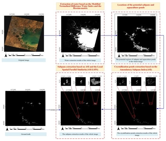
The Landsat-8 OLI data were utilized to study the extraction of saltpans with the existence of aquaculture ponds. They were downloaded from the USGS Center for Earth Resources Observation and Science (http://glovis.usgs.gov/ (accessed on 10 November 2022)). They have different geographical environments and characteristics regarding acquisition time and land cover types, as shown in Table 1. Seven bands are selected, including Coastal (0.43–0.45 μm), Blue (0.45–0.51 μm), Green (0.53–0.59 μm), Red (0.64–0.67 μm), and Near-infrared (0.85–0.88 μm) as well as Short infrared bands 1 (1.57–1.65 μm) and 2 (2.11–2.29 μm). To obtain high-quality and consistent experimental datasets, radiometric calibration and atmospheric correction have been performed through ENVI 5.3.
To develop the new saltpan index, we used the Google Earth map and visual inspection as references, and the reflectance values representing six typical land cover types along the coastal zone were selected, including crystallizing ponds, dams, the turbid water, dried-up reservoirs, tidal flats, and buildings. All samples were collected throughout 2021 in the coastal zones of China monthly. It is important to note that the samples were data from outside of the study areas. The crystallizing pond samples and the dried-up reservoir samples were only collected in northern China due to their special geographic distribution, while the other samples were evenly distributed among the coastal provinces of China. For each type of sample, 300 samples have been collected in each month, with a total of 21,600 samples sufficient to meet the requirements of spectral analysis to construct this new saltpan index.
To quantitatively evaluate the extraction results of saltpans, it is necessary to obtain the ground truth. Although in situ surveys could provide good accuracy, it is unsuitable and inconvenient to obtain the ground truth for extensive coverage. Thanks to the help of a panchromatic image (15 m resolution) and Google Earth map (2.17 m resolution), the ground truth images of saltpans could be manually delineated [20,21,22].

2.3. Methods

The flow chart of the proposed method is shown in Figure 2. The flow chart consists of four steps: (1) the extraction of water bodies, (2) the location of potential saltpans and aquaculture ponds regions, (3) the extraction of crystallization ponds, and (4) the extraction of evaporation ponds.
In the first step, a Modified Normalized Difference Water Index (MNDWI) [22] is used to extract the water body. Then, the linear structure of the dams is enhanced by using the Hessian matrix. In the second step, to roughly locate the regions of coastal saltpans and reduce calculations outside of them, the coastal regions containing saltpans have been extracted. In the third step, an Amendatory Saltpan Index (ASI) is presented to extract the crystallization ponds in saltpans. In the fourth step, evaporation ponds in saltpans are extracted by the local spatial parallel similarity criterion.

2.3.1. Extraction of Water Bodies

The MNDWI is one of the most widely used water indices for various applications, including surface water mapping, land use/cover change analyses, and ecological research [23]. To obtain water bodies, MNDWI [24] is used:
M N D W I = ρ G reen ρ S W I R 1 ρ G reen + ρ S W I R 1
where ρ G reen and ρ S W I R 1 are reflectance of the Green band and SWIR-1 band in Landsat-8, respectively. However, the direct application of the MNNWI water index method for water extraction may result in edge fracture in the dams of saltpans and aquaculture ponds. To enhance the structures of aquaculture ponds and saltpans, the Hessian matrix is used for the results by MNDWI. The Hessian matrix is a real symmetric square matrix composed of the second partial derivatives of a multivariate function. The eigenvalues and eigenvectors of it can be used to characterize the properties of specific structures (point structures/line structures) [25]. The eigenvalues and eigenvectors of a Hessian matrix could be described as a linear or tubular structure:
λ max = L x x + L y y + α 2
and
λ min = L x x + L y y α 2
where L xx , L yy , and L xy denote the second-order partial derivatives of x, y, and x-y in an image, respectively. α is a coefficient with α = ( L x x L y y ) 2 + 4 × L x y 2 . For linear structures, the eigenvalues of λ max are relatively large and of λ min are relatively small, while for nonlinear structures, the eigenvalue λ max is relatively small and λ min is rather large. Thus, the linear features of the dams could be enhanced by the Hessian matrix.

2.3.2. Location of Potential Saltpans and Aquaculture Ponds Regions

The usage of the Hessian matrix could retain the dam structure information well and refrain part of the dams from water bodies. However, it could bring many linear structural interferences, which may reduce extraction accuracy on saltpans and aquaculture ponds. To reduce the influence of linear interference, a direct approach is to extract the coastal zone including saltpans and aquaculture ponds. Since saltpans and aquaculture ponds are mainly distributed within 15 km of the coastline [26], the coastal zone containing these two kinds of ponds can extend 10 km from the coastline to land and 15 km from the coastline to the sea. To obtain such a zone, we obtained the rough coastline through MNDWI and expanded 500 pixels from the coastline to the left and right to obtain the coastal zone. Considering the resolution of Landsat-8 imagery, the usage of 500 pixels is sufficient to cover all coastal zones. Ultimately, all water bodies located in these zones could be used for further saltpans extraction.

2.3.3. Extraction of Crystallization Ponds

In this section, the crystallization ponds of saltpans can be extracted from the regions of saltpans and aquaculture ponds obtained from the previous section. Thanks to the high salinity of the crystallization ponds in the saltpans, the spectral characteristics of the crystallization ponds are different from those of the aquaculture ponds. However, only considering their spectral difference, a lot of interferences can appear in the whole image. To avoid this problem, in-depth spectral analysis of multiple land covers is required.
To visually analyze the spectrum of selected ground objects, the surface reflectance was derived from six typical ground samples to generate the spectral curves in Figure 3a, where we carried out average spectral analysis for each ground object. From the spectral curves, it can be inferred that the reflectance values of both the crystallizing ponds and turbid water gradually increase from band B1 to band B4, reaching a peak in band B4. Subsequently, there is a significant decrease in reflectance values in bands B5 and B6, followed by a slight decrease in band B7. Although peak reflectance values in the B4 band are exhibited by these two water bodies, significant differences between them are observed from the B3 and B4 bands. It can be clearly seen that although positive slopes are present in both spectral curves, the magnitude of the slopes differs significantly, with the crystallizing ponds exhibiting a noticeably larger slope than the turbid water, which constitutes the main spectral difference between them. Thus, (B4 − B3) can be considered as a good indicator distinguishing these two water bodies. However, it should be noted that in reality, a smaller slope in the B3 − B4 bands may also be observed in some crystallizing ponds with low brightness. In this case, a secondary difference between the two spectral curves should be considered: the average spectral values of the crystallizing ponds in the B7 and B4 bands are greater than those of the turbid water. Therefore, (B4 − B3) can be used as an indicator by assigning a larger weight, together with the usage of (B4 + B7) by a small weight to increase this difference. The reason for using the B7 band is that the average spectral value of the B7 band is the lowest among all bands, thereby allowing for a slight improvement to distinguish the above two water bodies while avoiding the introduction of additional interference. Additionally, it can be inferred from the spectral curve that the tidal flats exhibit spectral changes that conform to the aforementioned pattern. Hence, such usage can also be leveraged to eliminate tidal flats. At this point, interference from the turbid water has been eliminated.
However, some dams in aquaculture ponds still exist that can be regarded as interferences in the extraction of crystallization ponds. Upon observing the spectral response curves of the dams, it is noticed that the reflectance changes from B1 to B4 bands are similar to those of the crystallizing ponds. Moreover, the significant difference can also be seen from B5 to B7 bands, where the average spectral values of dams are obviously greater than those of the crystallizing ponds. Among these three bands, the greatest average spectral value difference between crystallizing ponds and dams can be seen in the B6 band. Furthermore, it can be seen from Figure 3a that the average spectral value of the crystallization ponds in B4 band is greatest than those in other six bands. In the B4 band, the mean reflectance of the dams is less than that of the crystallization ponds. Thus, using (B4 − B6) can expand this variation and effectively distinguish crystallizing ponds and dams. It is noteworthy that the average spectral value of buildings in the B6 band is also significantly greater than that of the crystallizing ponds. Therefore, most of the buildings can also be removed by this item. Consequently, the two main interferences, dams and turbid water, could be eliminated by exploiting the difference.
Nonetheless, the aforementioned indices cannot be used to distinguish the crystallization ponds and the dried-up reservoirs, as their spectral changes in these bands are remarkably similar. It is noted that the mean spectral values of dried-up reservoirs from band B1 to band B5 are greater than those of the crystallization ponds, as shown in Figure 3a. Therefore, a direct idea to distinguish crystallization ponds and dried-up reservoirs is to choose a band with the most pronounced difference between them. Clearly, it can be seen from Figure 3a that the average spectral value of the crystallization ponds in the B5 band is much lower than that of the reservoirs. However, it is not suitable to distinguish these two types of land cover using the B5 band. The reason is that dried-up reservoirs and crystallization ponds share the same surface reflectance by part from Figure 3b. It can be observed from Figure 3b that the best discrimination between the crystallization pond and the dried-up reservoir can be seen in B2. Ultimately, the B2 band is selected to differentiate these two types of land covers. Thus, the interference caused by dried-up reservoirs has also been removed.
According to the above analysis, an amendatory saltpan index (ASI) of Landsat-8 OLI images is proposed to maximize the difference between crystallization ponds and other similar water bodies, as
ASI = ( 3.44 × ρ red + 1.24 × ρ SWIR 2 2.2 × ρ green 0.25 ) × max ( 0 , ρ red ρ SWIR 1 0.1 ) × max ( 0 , 0.22 ρ b l u e )
where ρ r e d , ρ S W I R 2 , ρ g r e e n , ρ S W I R 1 , and ρ b l u e are the spectral reflectance values of Red, SWIR2, Green, SWIR1, and Blue bands in Landsat-8 OLI images, respectively. From (4), three parts on the right side of ASI can be seen. The first part produces positive values for crystallization ponds, while it yields negative values for turbid waters. Similarly, ( ρ red ρ S W I R 1 0.1 ) and ( 0.22 ρ b l u e ) generate a positive value for crystallization ponds and negative values for dams and dried-up reservoirs, respectively. The use of the max function in the second and third parts is to make sure that the ASI value for crystallization ponds is greater than 0, while the ASI value is less than or equal to 0 for non-crystallization ponds. The coefficients of ASI are the empirical results determined according to the spectral reflection values on various sample datasets with a similar track as [23]. ASI could be used to extract crystallization ponds and be free from the influence of dams and turbid water bodies, especially with aquaculture ponds nearby.

2.3.4. Extraction of Evaporation Ponds

As mentioned above, the crystallization ponds have been extracted through ASI. Then, the next step is to extract the evaporation ponds to complete the saltpans extraction in the entire imagery. Inspired by the alternating spatial distribution of the crystallization ponds and the evaporation ponds, where we find this characteristic in many saltpans in China, a local spatial similarity criterion is proposed to extract evaporation ponds with the existence of aquaculture ponds. The main idea could be summarized as (1) representing a single crystallization pond by a short line segment, (2) connecting short line segments in a neighborhood by a local connection strategy to form a long line segment representing a row of crystallization ponds, and (3) extracting evaporation ponds, by constructing the local spatial parallel similarity. The details of this extraction process can be illustrated as follows.

The Line Segment Presentation of a Single Crystallization Pond

First, any crystallization pond obtained from ASI is a polygonal body of water, which is difficult to describe macroscopically. Therefore, we use line segments to represent them. If each crystallization pond can be described by a line segment X i , then X = { X 1 , X 2 , , X i , , X N } represents the collection of line segments of all crystallization ponds extracted by ASI, where N is the number of crystallization ponds. For line segment X i , it can be described by five features, as X i = { c 1 i , c 2 i , l x i , l y i , θ i } , where c 1 i , c 2 i are the coordinates of the two endpoints of X i , l x i and l y i are the projections of the X i on the x-axis and y-axis, and θ i is the directional angle of X i . θ i is defined as the angle between the long axis of its ellipse with the same standard second-order central moment in the corresponding region of a straight line [27] and horizontal direction, with θ(θ∈(0, π)). c 1 i and c 2 i can be obtained by the intersection points between the major axis of the ellipse and the polygon of the crystal ponds, respectively.

The Connection of Parallel Line Segments

However, it is still difficult to describe the regional characteristic of crystallization ponds (i.e., a row of crystallization ponds). The reason is that these crystallization ponds are fractured by dams in geographical locations. Thus, it is necessary to connect line segments representing a row of crystallization ponds. The connections of such line segments are essentially equivalent to the connections of the endpoints with adjacent line segments by a connection criterion. Therefore, the endpoint set U = { U 1 1 , U 2 1 , , U 1 i , U 2 i , , U 1 N , U 2 N } is first established, where U 1 i and U 2 i represent the two endpoints of the X i , respectively.
Since there is only one dam between two adjacent crystallization ponds in a certain direction, the interval distance between adjacent line segments in parallel is generally short. If the endpoints of a line segment are known, we need to determine the set of endpoints for other line segments in its neighborhood. If we choose any endpoint U k 1 i of X i in U , with any other endpoint U k 2 j of X j , where k 1 and k 2 can be 1 or 2, representing the label for each endpoint, then we calculate the Euclidean distance D k 1 k 2 ij = c k 1 i c k 2 j between U k 1 i and U k 2 j . If D k 1 k 2 ij < = 20 is satisfied, U k 2 j is the endpoint that may need to be connected. Otherwise, we search for another endpoint. For U k 1 i , all endpoints that satisfy this Euclidean distance criterion can be constructed as a set U d i = { U m 1 i 1 , U m 2 i 2 , , U mn in } , where n represents the number of endpoints satisfying D k 1 k 2 ij < = 20 and m 1 , m 2 , mn can be 1 or 2, representing the label for each endpoint. In this regard, the threshold is set to 20 in pixels, based on the size of saltpans in Landsat-8 OLI imagery.
Moreover, adjacent line segments representing crystallization or evaporation ponds should have similar directionality. The connection rule here is defined as that the absolute value of the difference between directions of two line segments should be no more than 10 degrees. Moreover, the same type of adjacent line segments cannot overlap to avoid the wrong connection. In other words, the projections of these line segments in the horizontal and vertical directions are best not to overlap. The projections of the two segments in two directions overlapped should not exceed 2 pixels. Then, we need to determine the line segments in U d i that satisfy this criterion. If any endpoint of X j is in U d i , we need to judge whether X i and X j satisfy | θ i θ j | < = 10 (in degree) and l x i l x j < = 2 l y i l y j < = 2 (in pixels). If this criterion is satisfied, X j is retained; otherwise, X j is removed. All the line segments in U d i should be calculated by this criterion. Finally, the first endpoint in U d i is the best endpoint that we connect it with X i . Repeating this process for all unconnected endpoints, a row of crystallizing ponds can be represented by a long line segment. A row of crystallizing ponds refers to a group of crystallizing ponds with approximately the same direction and close proximity, which is macroscopically similar to a long line segment.

Evaporation Ponds Discrimination Criterion

In this section, we extract evaporation ponds according to the locations of crystallization ponds. After parallel line segments connection, the ponds of the same class with similar directions could be demonstrated as a long line segment. Due to the positions of evaporation ponds and crystallization ponds alternately distributed in parallel mode, the extraction of evaporation ponds could be completed according to the places of crystallization ponds. The ponds parallel to crystallization ponds with locations up or down are evaporation ponds. Therefore, to obtain the evaporation ponds, two rows of parallel crystallization ponds need to be located in advance. If each row of crystallization ponds can be described by a long line segment S i , then S = { S 1 , S 2 , , S i , , S M } represents the collection of long line segments for all rows of crystallization ponds, where M represents the total number of all single row of crystallization ponds. For S i , it can be described by two features, as S i = { L i , β i } , where L i is the length of S i , and β i represents the direction angle of S i . L i can be approximately calculated by the sum of short line segments in S i . β i can be approximately calculated by the average of the angles for all short segments in S i .
To find out two adjacent rows of crystallization ponds, their similar lengths could be utilized to construct a discriminant criterion. The criterion was defined as:
S I I S = exp ( L I L S L I )
where Ls and LI are the lengths of two long line segments in S , and LI is the longer one. Generally, depending on the architectural characteristics of actual saltpans, the length difference between Ls and LI is within half the length of LI, which satisfies the features of the alternating distribution of saltpans. Thus, LS satisfies 0.5 LI < LsLI. If Ls and LI are equal, S I I S should be 1. If the length of Ls tends to be half of LI, S I I S is 0.61. Thus, S I I S on two adjacent rows of crystallization ponds is between 0.61 and 1. In addition, if S p and S q denote any two rows of crystallization ponds, they should be approximately parallel, satisfying | β i β j | < = 10 . Only 0.61 < = S I pq < = 1 and | β p β q | < = 10 are satisfied, S p and S q can be used to represent two adjacent rows of crystallization ponds. Repeating the above process, we can determine all rows of crystallization ponds. Then, any two adjacent long line segments can be connected with four endpoints to form a closed region, which generally consists of two rows of crystallization ponds and one row of evaporation ponds. Thus, these evaporation ponds can be extracted directly since we know the regions on two rows of crystallization ponds. Repeating this process, all evaporation ponds can be extracted. Thus, the saltpans in the whole imagery can be extracted by ASI-LSPS.

2.3.5. Accuracy Assessment

To quantitatively evaluate the extraction performance of saltpans, the intersection over union (IOU) [28] and the Kappa coefficient [29] have been used as accuracy indicators. IOU refers to the overlap ratio between extracted result and ground truth [28], which can be expressed as:
IOU = T P TP + FP + FN
where TP means the number of correct-classified positive pixels, and FP means the number of miss-classified positive pixels. FN means the number of miss-classified negative pixels. The IOU represents the proportion of correct pixels accounting for total pixels, and we use IOU to evaluate the accuracy. The greater the value of IOU, the closer the experimental result is to the actual one.
The Kappa coefficient is also used to measure the extraction performance of the proposed method. In practical applications, the greater the Kappa coefficient, the better the method’s performance. The kappa coefficient can be expressed as:
Kappa = P 0 P e 1 P e
where P0 means the sum of the number of correctly classified samples for each class divided by the total number of samples and could be expressed as:
P 0 = TP + TN TP + TN + FP + FP
Pe means the sum of the product of the actual and predicted number corresponding to each category, divided by the square of the total number of samples, and could be expressed as:
P e = ( TP + FP ) × ( TP + FN ) + ( FP + TN ) × ( FN + TN ) ( TP + TN + FP + FN ) × ( TP + TN + FP + FN )

3. Results

In this section, three experiments were provided. First, the extraction results and performance comparison on crystallization ponds were presented by proposed ASI, NDSI [2], and Zhang’ s method [16] (named as ZBP). Second, the extraction results and performance comparison on saltpans were compared with the proposed ASI-LSPS, NDSI, and the method proposed by Hu et al. [15] (named as HPCA). Third, the saltpans extraction results of whole imagery in Tianjin and Shandong, China, were provided by the ASI-LSPS algorithm. As for the parameter setting of NDSI, we try our best to select the best thresholds. We have chosen the threshold as 0.11 and 0.13 in Tianjin and Dongying, China, respectively, with the principle of maximizing the retention of crystallization ponds while minimizing interference. As to ZBP’ s method, we set the output with two neutrons to highlight the extraction of crystallization ponds, and the rest of the parameters were the same as recommended. As to HPCA method, we just used recommended parameters used in that piece of literature.

3.1. Extraction Performance Comparison of Crystallization Ponds

In this section, three study sites with diverse geographical environments were chosen to assess the effectiveness of the proposed ASI in extraction of the crystallization ponds, in comparison with ZBP and NDSI. The first site is Tianjin; the second and the third sites are the two regions in Dongying, Shandong. Saltpans and aquaculture ponds coexist in these regions. Additionally, there are notable differences in the spatial distribution of the saltpans. In Tianjin, saltpans demonstrated a concentrated distribution that could be seen in the first column in Figure 4a, with red coloration for crystallization ponds. Still, saltpans were scattered in Dongying, as shown in the first column of Figure 4b,c.
Intuitively, three methods can be relatively complete extraction crystallization ponds. Nevertheless, some turbid water, dams, and dried-up reservoirs were extracted as crystallization ponds of saltpans by NDSI, marked by yellow circles in the second column of Figure 4a,b. In comparison with NDSI, the phenomenon of incorrect extraction by ZBP’s method was significantly reduced, but some turbid water and dams were still extracted as crystallization ponds, as shown by the yellow circles in the third column of Figure 4a,b. However, in the fourth column of Figure 4a,b, ASI can effectively distinguish crystallization ponds from the other three types of interference, marked by yellow circles. It could be seen from the second, the third, and the fourth columns in Figure 4c that the difference of extraction among three methods was not significant, because the water quality of aquaculture ponds is relatively clear and the dams in the aquaculture ponds are unaffected by turbid water. It can be concluded that the proposed ASI can outperform the other two algorithms with the existence of turbid water.
To quantitatively evaluate the extraction performance of crystallization ponds among NDSI, ASI, and ZBP, IOU and Kappa coefficients in these three regions have been used as shown in Table 2. The three regions a, b, and c correspond to the images in the first column of Figure 4 in sequence. It is evident that there is little difference extracting crystallization ponds at these three sites between ASI and ZBP methods. The differences in them for IOU and Kappa were less than 3%. However, ZBP required a substantial number of spectral samples as the trained dataset, which was a subjective and time-consuming step. However, in contrast to NDSI, ASI demonstrated better results. In region a, ASI outperforms NDSI by around 13% in IOU and by 14% in Kappa. The main reason is that NDSI can extract turbid water and some dams in the extraction of crystallization ponds, while ASI can avoid such problems. In region b, ASI is superior to NDSI by around 11% in IOU and around 10% in Kappa. The main reason is that NDSI can extract dry reservoirs and some dams in the extraction of crystallization ponds, while ASI can avoid such problems. In region c, the performance of ASI is better than that of NDSI by around 8% in IOU and around 6% in Kappa, since the spectral differences between aquaculture ponds and crystallization ponds are obvious. Therefore, ASI demonstrated better performance than NDSI and was a little superior to ZBP.

3.2. Performance Comparison of Saltpans Extraction

To evaluate the effectiveness of the ASI-LSPS algorithm in saltpans extraction, ASI-LSPS was compared with HPCA and NDSI. The sites in Section 3.1 have also been used, as shown in the first column of Figure 5a–c. Obviously, NDSI fails to effectively extract the evaporation ponds as shown in the yellow circles in the second column in Figure 5b,c. The reason is that NDSI could not distinguish low salinity water in evaporation ponds from other seawater, such as water in aquaculture ponds. Compared with the extraction results of NDSI, the saltpans were better extracted by HPCA, marked by yellow circles in the third column in Figure 5b,c, but many aquaculture ponds were mistakenly identified as saltpans. This is probably because HPCA solely relied on whether the spectral values in the near-infrared band were close to zero to distinguish evaporation ponds from other water bodies. As a result, HPCA can be ineffective when the spectral values in these bands of evaporation ponds are close to zero. However, ASI-LSPS could be used to extract most evaporation ponds that cannot be efficiently extracted by NDSI, marked by yellow circles in the fourth column in Figure 5b,c. Meanwhile, compared to HPCA, ASI-LSPS uses the local alternate distribution between evaporation and crystallization ponds for extracting the evaporation ponds that can be more reliable than the utilization of spectral differences. Overall, the extraction results of Figure 5 indicate that the saltpans can be effectively extracted by ASI-LSPS, while the use of the local parallel line criterion avoids interference from other water bodies.
To quantitatively evaluate the extraction accuracy of saltpans among ASI-LSPS and the other two algorithms, IOU and Kappa coefficients have been utilized, and the results are shown in Table 3. The IOU and Kappa coefficients of ASI-LSPS are at least 10% greater than those of other two algorithms since evaporation ponds cannot be well extracted by NDSI and HPCA’s methods. IOUs of ASI-LSPS are around 83% in Tianjin and Dongying, and Kappa coefficients are about 90%. It is proven that ASI-LSPS could effectively extract evaporation ponds in saltpans. Therefore, saltpans could be completely extracted by ASI-LSPS, demonstrating that ASI-LSPS has a good application prospect in coastal saltpans extraction.

3.3. Extraction of Saltpans in the Whole Imagery

Landsat-8 OLI images could cover a wide range and have large spectral differences in various regions. Therefore, saltpans extraction from a whole image is a challenging task. To verify the extraction of saltpans by ASI-LSPS in the entire imagery, we used the whole images based on the study areas in Tianjin and Shandong, China. As shown in the second column of Figure 6a,b, most saltpans in the above two study areas can be efficiently extracted. It indicates that ASI-LSPS performs well in saltpans extraction in all the Landsat-8 OLI images.

4. Discussion

In this paper, a saltpans extraction algorithm based on the amendatory normalized difference saltpan index and local similarity criterion by the alternate distribution of crystallization and evaporation ponds is proposed.
This algorithm is verified in the selected study areas. The results have shown that it could extract saltpans in the whole imagery with different geographical distribution characteristics for the first time, which could provide important information for monitoring and managing the coastal salt industry and ecosystem. In this section, the factors affecting the extraction accuracy of saltpans are first analyzed experimentally. Then, the uncertainty and limitation of the ASI-LSPS algorithm in the process of saltpans extraction still need to be discussed in detail.

4.1. The Impact of Seasonal Changes on the Extraction of Saltpans

Although ASI-LSPS can be used to extract saltpans effectively, there are still uncertain factors affecting the extraction accuracy. In the production of sea salt, the evaporation ponds have strict demands on light and temperature, leading to different spectral information at saltpans in different seasons. To study the impact of the ASI-LSPS algorithm in saltpans extraction under different seasons, we selected images of different seasons in Tianjin, China. In winter, the temperature in this region is often below zero degree Celsius, and certain water surfaces freeze. An ice surface and crystallization ponds demonstrate similar spectral characteristics, resulting in regions with ice being misclassified as saltpans, as indicated by the yellow circle in Figure 7d. During the spring season, the temperature is still low, but the majority of ice in the region has already melted. Consequently, even though the salinity of the crystallization ponds is low during this period, its extraction performance remains high, as illustrated in the third column of Figure 7a. During the summer season, the production of salt from crystallization ponds reaches its peak. As a result of the high temperatures, the rate of water evaporation from the ponds is accelerated, and the concentration of salt continually grows, which causes an increase in the spectral difference between saltpans and other ground objects such as aquaculture ponds. Therefore, as depicted in Figure 7b, the extraction performance is best in summer. In autumn, the production period for salt comes to a close. As the temperature drops, the rate of evaporation in saltpans slows down, resulting in a slight decrease in the extraction performance of the saltpans, as shown in Figure 7c. Thus, ASI-LSPS has the best extraction performance in summer, followed by a slight decrease in performance in spring and autumn and the lowest performance in winter.
To intuitively study the impact on the performance of ASI-LSPS algorithm with four seasons, IOU and Kappa coefficients have been used for quantitative analysis, as shown in Figure 8. IOU in summer is greater than 80%. Similarly, Kappa coefficients in summer are around 90%. The IOU coefficients for both spring and autumn can be greater than 75%, and the Kappa coefficient is around 85%. The IOU and Kappa coefficients in winter decrease by approximately 10% in comparison to those of other seasons. The higher the value of the IOU and Kappa coefficient, the better the performance. Hence, the results show that the ASI-LSPS algorithm has better saltpans extraction performance in summer, while the extraction performance is reduced in winter because of sea ice.

4.2. Advantages, Limitations, and Potential Improvements

4.2.1. Advantages

In the coastal zone, the extraction of saltpans is a challenging task due to several aquaculture ponds adjacent to saltpans. The advantages of the proposed ASI-LSPS can be divided into three aspects.
First, the proposed ASI in ASI-LSPS can greatly reduce the interferences such as turbid water, some dams, and dried-up reservoirs in the extraction of crystallization ponds in saltpans, which is very important for the whole imagery, while the compared algorithms cannot solve these problems that can increase the amount of postprocessing work. Second, ASI-LSPS can efficiently extract evaporation ponds based on the local alternate distribution between evaporation and crystallization ponds, while the compared algorithms cannot extract them or make misjudgments as aquaculture ponds partially. Third, ASI-LSPS is an automatic method for saltpans extraction in the whole images, while comparing algorithms requires manual intervention, and some algorithms only considered the salt fields rather than the entire images. Therefore, the ASI-LSPS algorithm can provide effective technical references for coastal resource utilization and production management in saltpans.

4.2.2. Limitations

Despite the advantages of ASI-LSPS in saltpans extraction, there are still four issues that need further investigation. (1) The inevitable occurrences of omissions and errors in the extraction results still can be seen. First, part of the aquaculture ponds located near the saltpans was mistakenly extracted by ASI-LSPS, as indicated by the pink circles in the fourth column of Figure 5a–c. This was caused by the adjacent rectangular spatial characteristics on adjacent saltpans and aquaculture ponds, which led to incorrect extraction results by the local alternate distribution.
Moreover, the occurrences of omissions and errors in ASI are such that ASI treats each crystallization or evaporation pond as an object and calculates the average spectral information of all pixels in this object. Due to the low sensor resolution, the dam information is fuzzy, which has led to the connection of some saltpans with other types of ponds, reducing the average values of spectral information in saltpans and making ASI identify such objects incorrectly.
Furthermore, the occurrences of omissions and errors based on local alternate distribution in ASI-LSPS are such that some small saltpans with only single-row crystallization ponds fail to meet the requirement of regular alternation of crystallization and evaporation ponds, resulting in the missing of the evaporation ponds.
(2) It is key to choosing suitable parameters. ASI has relatively stable thresholds. Two global thresholds have been used, with a parameter of 20 pixels controlling the connection between the two endpoints with the Euclidean distance and with a parameter as 10 degrees in the absolute difference value in angle between two line segments. The former parameter is suggested not to be small. The required crystallization pond may not be found. If it is too large, incorrect connections may occur. As to the latter parameter, if this parameter is too small, the required crystallization pond may not be found, and if it is too large, the crystallization pond in the other row may be connected causing incorrect connection.
(3) Clouds often appear in optical remote sensing images due to the influence of the weather. Clouds could directly affect the extraction accuracy of coastal saltpans. The reason is that the thick cloud layer makes the ground characteristics of saltpans fuzzy and spectral information is weakened.
(4) It is noteworthy that the estuary of the Yellow River is situated in Dongying, with significant sediment accumulation in this region, which alters the spectral characteristics of surrounding water bodies and results in incorrect extraction as saltpans, as illustrated by the yellow circle in the second column of Figure 6b.
The above problems need to be improved in future studies.

5. Conclusions

To solve these problems in coastal saltpans extraction, this paper proposed an ASI-LSPS algorithm based on amendatory saltpan index and local spatial parallel similarity by the alternate distribution of evaporation ponds and crystallization ponds. To verify the effectiveness of the ASI-LSPS, Landsat-8 OLI image data were used. In terms of crystallization pond extraction, the experiment shows that ASI can reach at least 70% in IOU and 78% in Kappa for the extraction of crystallization and demonstrates least 6% superiority over NDSI in Kappa and IOU. Meanwhile, ASI is almost as much as ZBP in Kappa and IOU. For saltpans extraction, experiments demonstrate that ASI-LSPS can reach at least 82% in IOU and 89% in Kappa in saltpans extraction, at least 13% and 17% better than the comparison algorithms in IOU and Kappa, respectively. In this regard, ASI-LSPS is an efficient method to extract saltpans in the whole imagery. Despite three advantages of ASI-LSPS, several limitations have to be considered. Therefore, future work will focus on studying the extraction algorithms to solve these problems.

Author Contributions

X.J.: software, validation, visualization, data curation, and writing—original draft preparation; X.S.: conceptualization, methodology, formal analysis, writing—review and editing, supervision, and funding acquisition; Z.S.: software, validation, visualization, data curation, and writing—original draft preparation; K.N.: methodology, software, validation, and formal analysis; Z.D.: formal analysis, investigation, and writing—original draft preparation. All authors have read and agreed to the published version of the manuscript.

Funding

This research was funded by Dalian Science and Technology Innovation Project, Dalian Science and Technology Bureau, P.R.C., grant number 2020JJ27SN101. It was also funded by Marine Environmental Monitoring Centre Project, P.R.C., grant number 2020Z0337.

Data Availability Statement

Not applicable.

Acknowledgments

The authors would like to thank the anonymous reviewers for their helpful and constructive comments.

Conflicts of Interest

The authors declare no conflict of interest.

References

  1. Oren, A. Saltern evaporation ponds as model systems for the study of primary production processes under hypersaline conditions. Aquat. Microb. Ecol. 2009, 56, 193–204. [Google Scholar] [CrossRef]
  2. Sridhar, P.N.; Surendran, A.; Ramana, I.V. Auto-extraction technique-based digital classification of saltpans and aquaculture plots using satellite data. Int. J. Remote Sens. 2008, 29, 313–323. [Google Scholar] [CrossRef]
  3. Wang, H.; Xu, X.G.; Zhu, G.R. Landscape Changes and a Salt Production Sustainable Approach in the State of Salt Pan Area Decreasing on the Coast of Tianjin, China. Sustainability 2015, 7, 10078–10097. [Google Scholar] [CrossRef]
  4. Bechor, B.; Sivan, D.; Miko, S.; Hasan, O.; Grisonic, M.; Radić Rossi, I.; Lorentzen, B.; Artioli, G.; Ricci, G.; Ivelja, T.; et al. Salt pans as a new archaeological sea-level proxy: A test case from Dalmatia, Croatia. Quat. Sci. Rev. 2020, 250, 106680. [Google Scholar] [CrossRef]
  5. Ri, P.V.; Stieglitz, T. Dry Season Salinity Changes in Arid Estuaries Fringed by Mangroves and Saltflats. Estuar. Coast. Shelf Sci. 2002, 54, 1039–1049. [Google Scholar]
  6. Albuquerque, A.M.; Ferreira, T.O.; Romero, R.E.; de Souza, V.S.; da Silva Júnior, C.A.B.; de Andrade Meireles, A.J.; Otero, X.L. Soil genesis on hypersaline tidal flats (apicum ecosystem) in a tropical semi-arid estuary (Ceará, Brazil). Soil Res. 2014, 52, 140. [Google Scholar] [CrossRef]
  7. Velasquez, C.R. Managing Artificial saltpans as a Waterbird Habitat: Species’ Responses to Water Level Manipulation. Colon. Waterbirds 1992, 15, 43–55. [Google Scholar] [CrossRef]
  8. Takekawa, J.Y.; Miles, A.K.; Schoellhamer, D.H.; Athearn, N.D.; Saiki, M.K.; Duffy, W.D.; Kleinschmidt, S.; Shellenbarger, G.; Jannusch, C.A. Trophic Structure and Avian Communities across a Salinity Gradient in Evaporation Ponds of the San Francisco Bay Estuary. Hydrobiologia 2006, 567, 307–327. [Google Scholar] [CrossRef]
  9. Giosa, E.; Mammides, C.; Zotos, S. The importance of artificial wetlands for birds: A case study from Cyprus. PLoS ONE 2018, 13, e0197286. [Google Scholar] [CrossRef] [Green Version]
  10. Cao, K.; Ma, H.W.; Sun, A.N. Analysis of spatial pattern for coastal salt pond engineer based on high spatial resolution satellite remote sensing imagery:a case study in south coast of Yingkou. J. Appl. Oceanogr. 2017, 36, 286–294. [Google Scholar]
  11. Wang, J.J.; Zhang, Y.; Tao, F. The Research and Application of the Salt Pan Water Area Classfication Method by Meams of Remote Sensing Classification of Saltpan Water. Ocean Technol. 2005, 24, 67–71. [Google Scholar]
  12. Arvor, D.; Daher, F.R.G.; Briand, D.; Dufour, S.; Rollet, A.; Simoes, M.; Ferraz, R. Monitoring thirty years of small water reservoirs proliferation in the southern Brazilian Amazon with Landsat time series. ISPRS J. Photogramm. Remote Sens. 2018, 145, 225–237. [Google Scholar] [CrossRef]
  13. Roy, D.P.; Wulder, M.A.; Loveland, T.R.; Woodcock, C.E.; Allen, R.G.; Anderson, M.C.; Helder, D.; Irons, J.; Johnson, D.; Kennedy, R.; et al. Landsat-8: Science and product vision for terrestrialglobal change research. Remote Sens. Environ. 2014, 145, 154–172. [Google Scholar] [CrossRef] [Green Version]
  14. Anshuman, B.; Joshi, P.; Snehmani, L.S.; Mritunjay, K.S.; Shaktiman, S.; Rajesh, K. Applicability of landsat8 data for char-acterizing glacier facies and supraglacial debris. Int. J. Appl. Earth Obs. Geoinf. 2015, 38, 51–64. [Google Scholar]
  15. Hu, P.X.; Zhang, Y.; Wang, J.H. Principal component fusion-based classification of salt field water bodies with remote sensing technique. J. Hohai Univ. Nat. Sci. 2004, 5, 519–522. [Google Scholar]
  16. Zhang, X.K. The Artificial Neural Network and Its Research on Classifying in Remote Sensing Image of Salt Fields Water. J. Salt Chem. Ind. 2006, 4, 40–43. [Google Scholar]
  17. Yu, Y.G.; Ma, Y. Spot-5 image marks for interpreting the types of land use/cover in the coastal zone of the Jiaozhou Bay. Coast. Eng. 2011, 30, 61–70. [Google Scholar]
  18. Lorenz, C.; Carlsen, I.; Buzug, T.M.; Fassnacht, C.; Weese, J. Multi-scale line segmentation with automatic estimation of width, contrast and tangential direction in 2D and 3D medical images. In Proceedings of the First Joint Conference, Computer Vision, Virtual Reality and Robotics in Medicine and Medical Robotics and Computer-Assisted Surgery, Grenoble, France, 19–22 March 1997; Springer: Berlin/Heidelberg, Germany, 1997; pp. 233–242. [Google Scholar]
  19. Liu, X.H.; Liu, L.; Peng, Y. Ecological zoning for regional sustainable development using an integrated modeling approach in the Bohai Rim. China. Ecol. Model. 2017, 353, 158–166. [Google Scholar] [CrossRef]
  20. Xie, L.; Zhang, H.; Wang, C.; Chen, F. Water-Body types identification in urban areas from radarsat-2 fully polarimetric SAR data. Int. J. Appl. Earth Obs. Geoinf. 2016, 50, 10–25. [Google Scholar] [CrossRef]
  21. Zhao, H.; Chen, F.; Zhang, M. A Systematic Extraction Approach for Mapping Glacial Lakes in High Mountain Regions of Asia. IEEE J. Sel. Top. Appl. Earth Obs. Remote Sens. 2018, 11, 2788–2799. [Google Scholar] [CrossRef]
  22. Zhang, G.; Zheng, G.; Gao, Y.; Xiang, Y.; Lei, Y.; Li, J. Automated water classification in the Tibetan Plateau using Chinese GF-1 WFV data. Photogramm. Eng. Remote Sens. 2007, 83, 33–43. [Google Scholar] [CrossRef]
  23. Feyisa, G.L.; Meilby, H.; Fensholt, R.; Proud, S.R. Automated Water Extraction Index: A new technique for surface water mapping using Landsat imagery. Remote Sens. Environ. 2014, 140, 23–35. [Google Scholar] [CrossRef]
  24. Mcfeeters, S.K. The use of the Normalized Difference Water Index (NDWI) in the delineation of open water features. Int. J. Remote Sens. 1996, 17, 1425–1432. [Google Scholar] [CrossRef]
  25. Aylward, S.R.; Bullitt, E. Initialization, Noise, Singularities, and Scale in Height Ridge Traversal for Tubular Object Centerline Extraction. IEEE Trans. Med. Imaging 2002, 21, 61–75. [Google Scholar] [CrossRef] [PubMed]
  26. Sun, Z.; Luo, J.; Yang, J.; Yu, Q.; Zhang, L.; Xue, K.; Lu, L. Nation-Scale Mapping of Coastal Aquaculture Ponds with Sentinel-1 SAR Data Using Google Earth Engine. Remote Sens. 2020, 12, 3086. [Google Scholar] [CrossRef]
  27. Xia, G.; Delon, J.; Gousseau, Y. Shape-based Invariant Texture Indexing. Int. J. Comput. Vis. 2010, 88, 382–403. [Google Scholar] [CrossRef]
  28. Richards, J.A. Image Classification in Practice. In Remote Sensing Digital Image Analysis; Springer: Berlin/Heidelberg, Germany, 2013; pp. 381–435. [Google Scholar]
  29. Shi, T.Y.; Zou, Z.; Shi, Z.; Chu, J.; Zhao, J.; Gao, N.; Zhang, N.; Zhu, X. Mudflat aquaculture labeling for infrared remote sensing images via a scanning convolutional network. Infrared Phys. Technol. 2018, 94, 16–22. [Google Scholar] [CrossRef]
Figure 1. The locations of the study regions. Two red rectangles can be seen in the bottom left figure, where the upper one refers to Tianjin region, China, and the lower one refers to Dongying region, China.
Remotesensing 15 03413 g001
Figure 2. Flowchart of the proposed method for saltpans extraction.
Remotesensing 15 03413 g002
Figure 3. Spectral comparison of different land cover types. (a) The mean spectral curves of the six typical coastal ground objects, where each point denotes the average reflectance with all samples of each type in one band. (b) The comparison of the bar chart of dried-up reservoirs and crystallizing ponds from band B1 to band B7 by all samples in both types. For each bar chart, the positions of the 10th and 90th percentiles are displayed using level lines, and the range from the 25th percentile (Q1) to the 75th percentile (Q3) is represented by the box in the box plot. The circles indicate the 5th, 50th, and 95th percentiles.
Remotesensing 15 03413 g003
Figure 4. The extraction results of the crystallization ponds using ASI, ZBP, and NDSI methods, with (a), (b), and (c) representing the ground truth and results in the sites, corresponding to Tianjin, Dongying 1, and Dongying 2, respectively. The first column were the ground truths of crystallization ponds in Tianjin, Dongying 1, and Dongying 2, where the crystallization ponds are highlighted in red coloration. The second, third, and fourth columns are extraction results of crystallization ponds by NDSI, ZBP, and the proposed ASI, respectively, in Tianjin, Dongying 1, and Dongying 2, where blue represents crystallization ponds, green indicates an omission error, and red is used for commission errors. The yellow circles highlight the interferences (i.e., turbid water, dams, and dried-up reservoirs) suppression results of each method.
Remotesensing 15 03413 g004
Figure 5. The performance comparison for extraction of saltpans by the proposed ASI-LSPS, NDSI, and HPCA, with (a,b), and (c) representing the ground truth and results in the sites, corresponding to Tianjin, Dongying 1, and Dongying 2, respectively. The first column is the ground truth of saltpans, with red representing saltpans. The second, third, and fourth columns are extraction results of saltpans by NDSI, HPCA, and ASI-LSPS, respectively, where blue, red, and green colors represent correctly extracted, incorrectly extracted, and omitted saltpans, respectively, and black coloration represents non-saltpans. The yellow circles highlight the extractions of evaporation ponds for each method. The pink circles highlight the aquaculture ponds mistakenly extracted as the saltpans for each method.
Remotesensing 15 03413 g005
Figure 6. The extraction results of ASI-LSPS with the whole images, with (a) and (b) representing the false-color images and the results in Tianjin and Dongying, China, respectively. The first column is false-color images in red, green, and blue bands of Tianjin and Donging, respectively. The second column is their saltpans extraction results by ASI-LSPS, where regions with blue, red, and green colors represent correctly extracted, incorrectly extracted, and not extracted saltpans, respectively. The region with black coloration represents non-saltpans. The yellow circle highlights the estuary region mistakenly extracted as the saltpans by ASI-LSPS.
Remotesensing 15 03413 g006
Figure 7. Extraction results of saltpans with four seasons in Tianjin, China, with false-color images in red, green, and blue bands in the first column, ground truth in the second column, and saltpans extraction results in the third column. (a) In spring; (b) In summer; (c) In autumn; (d) In winter. In the second column, red in ground truth represents saltpans. In the third column, blue, red, and green colors represent correctly extracted, incorrectly extracted, and omissive saltpans, respectively. Black coloration represents areas that are non-saltpans. The yellow circle highlights the ice surface mistakenly extracted as saltpans.
Remotesensing 15 03413 g007aRemotesensing 15 03413 g007b
Figure 8. The impacts of seasonal changes of ASI-LSPS on IOU and Kappa in Tianjin, China.
Remotesensing 15 03413 g008
Table 1. The metadata and major types in landscapes of Landsat-8 OLI.
Study AreaLandsat-8 Scene IDPath/RowData
Acquisition
Cloud CoverSite CenterMajor Types of Landscapes
aLC81220332019302LGN00122/3328 October 20191.06%38°55′52.04″N, 117°53′1.88″ESaltpans,
aquaculture ponds,
vegetation,
artificial buildings, and mangrove forests
LC81220332019014LGN00122/3314 January 20190.55%38°55′52.04″N, 117°53′1.88″E
LC81220332019078LGN00122/3319 April 20194.1%38°55′52.04″N, 117°53′1.88″E
LC81220332019270LGN00122/3327 September 20192.96%38°55′52.04″N, 117°53′1.88″E
LC81220332019318LGN00122/3314 November 20193.24%38°55′52.04″N, 117°53′1.88″E
bLC81210342019199LGN00121/3418 July 20199.43%37°29′33.75″N, 118°59′47.89″ESaltpans, aquaculture ponds, bare ground, artificial buildings, vegetation, and crops
Table 2. Accuracy evaluation of the proposed ASI, NDSI, and ZBP methods on the extraction of crystallization ponds in Tianjin and Shandong, China.
Study
Regions
ASINDSIZBP
IOU (%)Kappa (%)IOU (%)Kappa (%)IOU (%)Kappa (%)
a0.71750.80910.58280.66310.70230.7914
b0.70510.78530.59430.68450.68090.7712
c0.73650.83810.65660.77880.72950.7953
Table 3. Accuracy evaluation on saltpans extraction among three methods in Tianjin and Dongying, China.
Study
Regions
ASI-LSPSNDSIHPCA
IOU (%)Kappa (%)IOU (%)Kappa (%)IOU (%)Kappa (%)
a0.85670.89160.54420.62350.60110.6521
b0.82360.89690.51230.59640.66090.7183
c0.84620.90960.55560.67020.70950.7353
Disclaimer/Publisher’s Note: The statements, opinions and data contained in all publications are solely those of the individual author(s) and contributor(s) and not of MDPI and/or the editor(s). MDPI and/or the editor(s) disclaim responsibility for any injury to people or property resulting from any ideas, methods, instructions or products referred to in the content.

