Article

A Study of the Relationships between Depths of Soil Constraints and Remote Sensing Data from Different Stages of the Growing Season

School of Agriculture and Food Science, The University of Queensland, St Lucia, QLD 4072, Australia
*
Author to whom correspondence should be addressed.
Remote Sens. 2023, 15(14), 3527; https://0-doi-org.brum.beds.ac.uk/10.3390/rs15143527
Submission received: 18 May 2023 / Revised: 9 July 2023 / Accepted: 10 July 2023 / Published: 13 July 2023

Abstract

:
The presence of salinity and sodicity in the root zone can limit root development and impact crop yield. Topsoil constraints are likely to have the greatest impact on crop growth early in the growing season, when plant roots are still shallow. Later in the growing season, subsoil constraints may have a greater impact as roots reach deeper into the soil. This study investigated whether different patterns of spatial variation in crop growth would be evident in remote sensing data captured from different stages of the growing season, with the aim of providing a means of indicating whether soil constraints in the topsoil and in the subsoil might be impacting crop growth. If a topsoil constraint is impacting growth, we might expect its effects to show through a negative correlation between the soil constraint and the early-season vegetation index. However, we would not expect to observe the impact of a subsoil constraint until later in the season (when roots have reached the constraint). To test the results from the analysis of remote sensing data, we used soil data from five fields from across Australia’s northern grains-growing region. We used these data to assess soil constraint severity and correlations between the soil constraints and enhanced vegetation index (EVI). The results of the study were inconclusive, and it was difficult to identify a dominant soil constraint with a clear relationship to crop growth. The soil data were also insufficient to draw conclusions about the depths of any dominant soil constraints. Furthermore, there was a lot of subjectivity in the interpretations of the correlations between remote sensing and soil data. The study also investigated the consistency of the spatial variation in EVI over multiple years, but the results were still inconclusive. In conclusion, this study highlights the challenges of using remote sensing data to diagnose soil constraints in agricultural settings. While remote sensing can provide useful insights into crop growth, interpreting these data and drawing meaningful conclusions about soil constraints requires further research and development.

1. Introduction

Soil constraints are limiting factors affecting crop growth and negatively impacting worldwide agricultural production. It has been estimated that 76% of soils globally and 77% of those in Australia have single or multiple soil constraints [1]. In a large portion of a grains-growing region of eastern Australia, the major constraints that hinder agricultural productivity are linked to the salt levels in the soil, specifically salinity and sodicity [2]. For example, recent studies have estimated that 68% of wheat farmland in Australia is constrained by sodicity and 24% by salinity [3].
Soil salinity is characterized by a high quantity of soluble salts present in the soil solution [4,5], whereas soil sodicity is indicated by a high concentration of sodium ions (Na+) in the soil cation exchange complex (CEC) [6]. In general, plants can benefit from a moderate amount of soluble salt or sodium ions. However, excessive amounts of these elements can have detrimental effects on the soil, deteriorating soil structure, which can restrict soil water infiltration and storage [4,7,8,9]. Moreover, the excess of soluble salt or sodium ions may adversely affect soil function, limiting the plant root’s ability to access stored water and nutrients, impacting crop growth and causing yield decrease [4,6,7,10].
The salinity and sodicity severity can be distributed differently across regions. Moreover, the severity can also vary at a small scale across a field and within the soil profile. For example, in Australia, many studies find that salinity increases with profile depth [11,12,13]. This variability for both topsoil and subsoil may contribute to crop yield variation. However, it is not easy to evaluate the contribution of salinity and sodicity in different layers to crop growth. Therefore, many studies only assess topsoil and subsoil constraints’ contribution to crop yield separately [14,15].
The crop’s root-zone condition plays a vital role in crop growth. The presence of salinity and sodicity around the root zone possibly limits root developments, impacting crop yield [16]. As the plant grows, the roots reach deeper soil layers to exploit more water and nutrients. Early in the growing season, when the plant roots are still shallow, topsoil constraints would have the most potential to affect crop growth. Later in the growing season, when the plant roots have reached deeper, subsoil constraints would have the potential to impact crop growth.
Crop growth from emergence to maturity can be monitored and assessed using remote sensing data. In particular, the Landsat series of satellites offer the spatial and temporal resolution—Landsat 5, 7 and 8, with 30 m pixel sizes and with repeat intervals of 16 days and long periods of two satellites in operation simultaneously—to investigate changes in the within-field variation in crop growth through the growing season for the large broadacre cropping fields common in Australia’s grains-growing regions. The data can be used to calculate vegetation indices representing vegetation greenness and density [3,17,18,19,20,21,22,23,24,25]. This study used the enhanced vegetation index (EVI) [26], one of the several indices that was found to give a reasonable representation of within-field yield variation in the study area [27,28,29] to represent vegetation density for each growth stage from emergence to maturity.
This study investigated whether different patterns of spatial variation in crop growth would be evident in remote sensing data captured from different stages of the growing season, with the aim of providing an approach to indicate whether soil constraints in the topsoil or in the subsoil might be impacting crop growth. Existing datasets from five fields in the study region were analyzed, with soil data from across these fields compared with the remote sensing data. The aim in this study was to investigate whether this kind of analysis would be able to provide insights into how soil constraints might be impacting growth, and therefore whether similar analyses might be more broadly applicable. Therefore, the hypotheses in this study are as follows:
  • If a topsoil constraint is impacting growth, we might expect its effects to show through a negative correlation between the soil constraint and the early-season EVI.
  • We would not expect an impact of a subsoil constraint until later in the season (when roots have reached the constraint); therefore, subsoil constraints might show effects through negative correlations between the soil data and EVI from later in the growing season.
  • We investigated whether data from the five fields provide any support for these hypotheses, and therefore whether the type of analysis applied here might be more broadly applicable for diagnosing the depth of soil constraints impacting crop growth.

2. Materials and Methods

2.1. Study Area

The study area is located in the northern grains-growing region of Australia (as defined previously by the Grains Research and Development Corporation, GRDC), encompassing the central and southern areas of Queensland and the northern parts of New South Wales (Figure 1). The study concentrates on winter crops, predominantly wheat (and also barley) that is typically sown between April and July and harvested from September to December. Furthermore, during summer, with limited cropped years, sorghum is dominant [30]. The region experiences a semi-arid climate and is mainly utilized for winter grains cropping, with wheat being the predominant crop. In this study, data were collected from five dryland cropping fields located in the region and selected in earlier work [7,14,19,30,31,32] when soil sampling was conducted. The five fields range from 10 to 200 ha with elevation ranging from 190 to 320 m above sea level (3–15 m in-field topographic difference; 8.6 m for Field 1, 8.2 m for Field 2, 14.7 m for Field 3, 3.7 m for Field 4, 7.3 m for Field 5) [30]. Generally, the soils in this region are composed mainly of cracking clay soils (Vertosols) [6,14,19,30,32,33,34], with lesser occurrences of Sodosols [35] and Chromosols [36]. Specifically, the five selected fields are dominated by Vertosols.

2.2. Datasets and Pre-Processing

2.2.1. Satellite Data

The study utilized satellite imagery with a 30 m pixel resolution from Landsat-5 Thematic Mapper (TM), Landsat-7 Enhanced Thematic Mapper Plus (ETM+), and Landsat-8 Operational Land Imager (OLI), collected between 1999 and 2019. The surface reflectance was derived [37], and cloud and cloud shadow were removed using the Fmask algorithm [38]. The data from three bands of each satellite were used, namely blue, red, and near-infrared (NIR) of the electromagnetic spectrum, to compute the enhanced vegetation index (EVI, Equation (1)) [39], a parameter previously utilized in previous work [27,28,29] and proven to be reasonably correlated with crop yields in the study region. Imagery from between 1 April and 15 December was included, to span the winter cropping growth period in the region, and each image clipped to the field boundary. Only images with data covering at least 75% of the pixels of the field area were included. Incomplete images resulted from either (i) partial cloud coverage or (ii) the ‘SLC (Scan Line Corrector)-off’ problem with Landsat 7. To fill in gaps in incomplete images with ≥75% field coverage, we applied regression kriging as follows. First, the image (from the same season as the incomplete image) with the highest correlation to the incomplete image was selected as the covariate (provided it covered the missing pixels). Then, a linear model was applied to predict the missing pixels before the residuals from this linear model were kriged and added to the linear function to give the fill values. For each field, the resulting dataset consisted of a set of complete EVI rasters for multiple dates within each growing season from 1999 to 2019. To give EVI data representative of each of the four stages of the season (see Section 2.3.1), we temporally interpolated EVI to give a daily stack of EVI rasters, before aggregating the daily data to extract the mean EVI for each of the four stages.
E V I = 2.5   ( N I R R e d ) ( N I R + 6 × R e d 7.5 × B l u e + 1 )

2.2.2. Soil Constraint Data and Severity Index

In the analysis, we took into account the soil constraint data (Table 1) that were gathered in a previous work, where the sampling was carried out using a stratified random design, based on a preliminary electromagnetic induction survey, resulting in reasonably distributed locations [30]. We assumed the soil constraints were temporally stable over time from 1999 to 2019; that is, the spatial variation in soil constraints within the field when it was sampled in 2009 was reasonably similar to the spatial variation in those constraints over the whole considered period (1999–2019), although we acknowledge that this was not checked by resampling the soil in the field. Thus, in this analysis, we used one set of soil constraint measurements taken between April and May 2009 from eight to twelve sampled soil cores per field [30]. Each sampled core was split into eight depth intervals, and data from four of these depths are considered here: 0–10 cm, 30–50 cm, 70–90 cm, and 110–130 cm. The samples were dried at 40 °C in a forced-draught oven and ground to pass through a <2 mm sieve [30]. Two variables representing soil constraints, ESP (exchangeable sodium percentage) and ECse (electrical conductivity of a saturated paste extract, were used in this analysis. ESP indicates soil sodicity and possible dispersion effects, while ECse represents soil salinity. The ESP was calculated based on the ratio of exchangeable Na to CEC, determined using 1 M NH4Cl extracting solution. In the meantime, the ECse was calculated using the EC1:5 with the Cl and clay content [5]. Within fields, the sampled profiles exhibited significant variation in terms of these soil constraints.
To allow some comparison of different soil constraints in terms of their expected impacts on crop growth, the soil constraints dataset was converted to severity indices based on wheat crop tolerant limits. A study by Page et al. (2021) reviewed literature on the tolerance limits of different crops to different soil constraints, and compiled tolerance limits for potential and severe impacts of soil constraints [40] (Table 2); we applied these tolerance limits to calculate a severity index as follows. We gave the index of 1 to a soil constraint causing potential yield loss (according to the literature-derived values given in the second column of Table 2) and the index of 2 to a soil constraint causing severe yield loss (the third column of Table 2). We assumed an ‘extreme’ severity (giving the maximum index of 3) at twice the value of the ‘severe’ impacts, and ‘no constraints’ (a severity index of 0) at a value 0. In between the tolerance limits presented in Table 2, linear interpolation was applied to give a severity index (e.g., a measured value of subsoil ESP of 30% would give a severity index of 2.5). The final three columns of Table 1 give the summary of the resulting soil constraints severity index applied for the data in each of the five fields. The combined index is the maximum of the two individual severity indices for each sampled soil profile and depth, which we used as a way of investigating whether remote sensing will be able to reveal something about the depth of a dominant soil constraint.

2.3. Initial Data Processing Methods

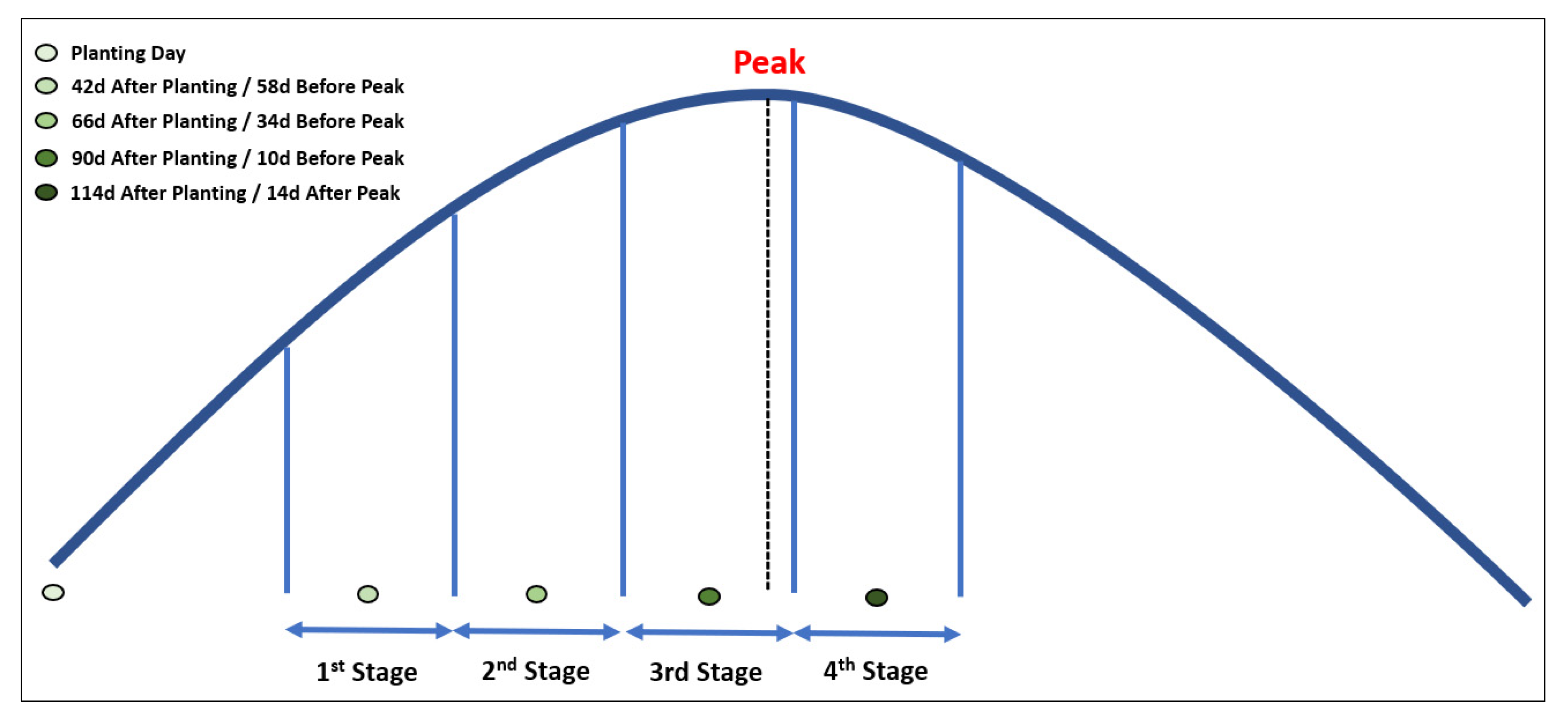
2.3.1. Dividing Crop Growth into Several Stages

This study examined the remote sensing data to assess topsoil and subsoil constraints in different crop growth stages. The stages were divided based on the estimated time when roots reached certain depths, including 30 cm (1st stage), 60 cm (2nd stage), 90 cm (3rd stage), and 120 cm (4th stage). During the first six weeks after planting, wheat roots grow up to 30 cm depth, then speed up to grow 1.25 cm per day [41,42]. Based on this, we assumed that wheat roots would reach 30 cm 42 days after planting (1st stage), 60 cm 66 days after planting (2nd stage), 90 cm 90 days after planting (3rd stage), and a depth of 1.2 m 114 days after planting (4th stage; Figure 2).
Based on the analysis of data (not shown) where the planting dates were known, the planting of a wheat crop in the region occurs around 100 days before the peak EVI (which corresponds with the greatest biomass period). Therefore, relative to the peak EVI, the date representing the 1st stage is centered around 58 days before the peak, the 2nd stage is around 34 days before the peak, the 3rd stage is around ten days before the peak, and the 4th stage is around 14 days after the peak. With 24-day windows representing each stage (12 days before and after the nominal date), the 1st stage is represented by the average EVI from imagery between 70 and 47 days before peak EVI, the 2nd stage from imagery from 46 to 23 days before peak EVI, the 3rd stage from imagery from 22 days before peak EVI until 2 days after peak EVI, and the 4th stage from imagery from 3 to 26 days after peak EVI (Figure 2). Thus, as described earlier in Section 2.2.1, the Landsat data were interpolated to a daily time step before aggregation to represent each of the four stages, resulting in four images of each field from each growing season from 1999 to 2019. Table 3 shows the date ranges representing each of the four stages, the expected root depth at this stage of the season, and the sampled depth from our dataset selected to represent constraints at that depth. A sampled soil depth of 0–10 cm was taken to represent the 1st stage (when roots might be expected to reach 30 cm depth), a soil depth of 30–50 cm to represent the 2nd stage (when roots reach 60 cm depth), a soil depth of 70–90 cm to represent the 3rd stage (when roots reach 90 cm depth), and soil depth of 110–130 cm to represent the 4th stage (when roots reach 120 cm depth).

2.3.2. Detecting Years to Be Included in the Ensuing Analysis

This analysis involved remote sensing data collected from 1999 to 2019. However, it would not be appropriate to utilize the remote sensing from all years in the analysis (concerning soil constraints). Some years may not have had crops planted (in growing seasons with limited ICR (In Crop Rainfall; it is common for growers to decide not to plant crops to avoid crop failure), while for other years, the remote sensing data may not have been enough to provide a confident spatial representation of crop growth and yield. Since we aimed to provide a means of analysis based on the remote sensing data, we defined a series of heuristics to detect the years included in the subsequent analysis. For each field, we calculated the field-median EVI for all available dates of imagery to compile a time series of field-median EVI for each year and checked that (i) there were at least five available dates in a certain year, (ii) the maximum field median EVI in a year was greater than 0.25, (iii) the maximum field-median EVI was between mid-June until the end of October (indicative of the peak biomass for a winter crop), (iv) the field-median EVI both before and after the time of the peak was at some point less than half of the maximum field-median EVI (an indication of a reasonably pronounced growth curve), and (v) the data from a growing season spanned a minimum of 120 days. In addition to these heuristics, we looked for evidence of spatially differential management in the imagery and excluded any seasons where such evidence was found. We only used data from fields that were managed uniformly to ensure that any spatial differences in crop growth were predominantly due to soil spatial variability rather than differential management.

2.4. Statistical Analysis Methods

2.4.1. Soil Constraints Severity and Vegetation Index Correlation

As an initial analysis, we used correlation analysis to investigate the general relationship between soil constraint and yield. In this analysis, we used the soil constraints severity index (combination of soil sodicity and salinity severity, see Section 2.2.2) to represent soil constraints and average EVI to represent the yield. The average EVI value was extracted from a single pixel where the soil sample was located. It is generated for a given stage over all the years (see Section 2.2.1). The soil constraint severity index is generated for four different sample depths (according to the depth where roots would be expected at the given stage) in each profile. Therefore, correlation values were examined between the average EVI and soil constraints severity index in different profiles (but at the same depth). In addition, we also calculate the correlation between each depth of soil constraints’ severity to the peak stage EVI, aiming to check whether soil constraints at other depths influences vegetation growth, especially during the peak biomass period.

2.4.2. Within-Field Variation in Soil Constraint Severity

The variation in the severity of soil constraints for a certain soil depth across a field should give an indication of the spatial variation that could be expected in their impact on crop growth. If there is little variation in severity for a given soil depth, we might expect little variation in crop growth (due to these constraints) at the stage of the season when roots would be expected to encounter these constraints. Meanwhile, if there is a large amount of variation in severity for a given soil depth, we might expect variation in growth at the stage of the season when roots would be at this soil depth. We used box plots to assess this variation in soil constraint severity, and therefore to indicate the potential of an analysis of remote sensing data (from a given stage) to show variation related to soil constraints data (from the corresponding soil depth).

2.4.3. Soil Constraints and Vegetation Index Correlation

Aside from the correlation analysis between soil constraint severity and average EVI, we also investigated simple relationships between individual soil constraints’ indicators and average EVI. The concept is similar to the correlation based on the soil constraints severity index (Section 2.4.1), where the correlations were assessed between four soil depths of individual soil constraints and the average EVI from relevant stages. These correlations were assessed for each field in turn, to investigate the within-field variation.

3. Results

The overall correlation between the soil constraints severity index and average EVI (from the corresponding stage of the season) showed a negative relationship. It is shown from the negative r values for almost every depth in each field, especially topsoil, until a depth of 70–90 cm (Table 4). The r values varied between −0.10 and −0.75. Even though the p-values are mostly not statistically significant, the negative values of the correlation at least aligned with the general concept where the more severe the soil constraints, the lower the average EVI.
For more detailed assessment, we investigated soil constraints severity index variation in different soil depths and correlations between individual soil constraint indicators to average the EVI of each soil sample location in different years. Field 1 showed very limited variation in the soil constraint severity index at the depth 0–10 cm and showed some variation at other depths (Figure 3a). This result suggests that it would be unlikely that variation in growth would be related to variation in topsoil constraints. This variation interpretation is also supported by the correlations between the individual constraints (ECse and ESP) and EVI from the 1st stage, which also showed no correlation (Figure 3b). However, some soil constraints’ severity variation was evident from the 30–50 cm sampled soil depth, which also correlated with 2nd stage EVI (r = −0.75; Table 4). Individual soil constraints (particularly ECse) from the 30–50 cm sampled soil depth also showed strong negative correlations with the 2nd stage EVI. The strongest correlation (r = −0.89) was between ECse at a depth of 30–50 cm and the average EVI during the 2nd stage (when roots might be expected to reach a depth of around 30–60 cm).
Some variation in soil constraint severity was shown in Field 2 from the topsoil to subsoil (Figure 4a). For the topsoil variation, the values of this index less than 1 would not be generally expected to give rise to yield loss. Nonetheless, there was a (insignificant) negative correlation between the severity index for 0–10 cm and the 1st stage EVI (r = −0.52, p = 0.23; Table 4). The correlation between 1st stage EVI and ECse was stronger than with ESP, meaning that any topsoil constraints affecting variation were more likely to be associated with salinity than with sodicity (Figure 4b). Considering the relationships between soil and EVI later in the season, the topsoil ECse showed its strongest correlation with the 4th stage EVI (−0.74), possibly aligned with topsoil salinity being the dominant constraint and having an effect on crop growth here throughout the season.
The severity index for Field 3 showed values less than 1 for all sampled locations across the field for the 0–10 cm, 30–50 cm and 70–90 cm soil depths (Figure 5a), which does not suggest that ECse or ESP are at the levels expected to result in yield loss. However, the soil constraint severity index showed more variation and higher values for 70–90 cm and 110–130 cm. From the correlation analysis, there was a strong negative correlation between all depths for ESP and EVI, perhaps a result of some of the sodicity effects at all soil depths, even at the values of topsoil ESP below those considered as indicative of potential constraints (ESP = 6%; Table 2). The correlations between ESP and EVI were quite strong for all depths and stages, with the strongest being for the ESP at 30–50 cm (r = −0.88, p = 0.02; Table 4).
For Field 4, the soil constraints severity index variation was slightly visible at the depth 0–10 cm, increased at the depth 30–50 cm, and no variation at all at the depth 70–90 cm and 110–130 cm. At the depth 70–90 cm and 110–130 cm (representing the expected root depth at the 4th stage), the severity was close to 3 (the extreme) across the field (Figure 6a). This lack of spatial variation in the severity index means that it cannot be used to test whether variation in growth aligns with variation in the subsoil constraints severity index (possibly the severity index, as we have defined it, is not sensitive enough to explain the growth here). It is supported by the correlation result between EVI and the individual soil constraints (ECse and ESP) for depth 110–130 cm, which showed a value close to 0 (Figure 6b). In addition, the correlations between the soil constraint severity index in this field for all the four sampled soil depths and the EVI were not statistically significant (Table 4). However, the strongest correlation between the soil constraint and EVI data was between ECse at 70–90 cm and the 4th stage EVI (r = −0.69). This correlation possibly indicates an effect of salinity at 70–90 cm depth due to high severity.
In addition, for Field 5, the severity variation shows that the largest variation across the field was at the depth 30–50 cm (Figure 7a). We might, in theory, expect this variation in severity to cause variation in growth. However, there was no relationship between soil constraint severity (at 30–50 cm) and EVI during the 2nd stage (Table 4). The correlation analysis (Figure 7b) shows negative correlations between soil constraints at a depth of 30–50 cm and average EVI in the 2nd stage (r = −0.41 for ECse, r = −0.20 for ESP), though these were not statistically significant. Although there are stronger correlations between the 2nd stage EVI and the 1.1–1.3 m ECse, roots should not be encountering this deeper salinity in the 2nd stage, so this should not be the direct cause of the growth variation observed in the 2nd stage. The correlation between ECse and 2nd stage EVI is greater than in the 1st stage.

4. Discussion

4.1. Correlation between Soil Constraint Severity Index and EVI

Statistically, the correlation analysis between soil constraints severity at each depth and average EVI at relevant stages showed some significant and some insignificant p-values. However, the overall relationship between soil constraints severity and average EVI is negatively correlated, especially for the topsoil until a 90 cm depth. This result aligned with the general hypothesis that the higher the severity of soil constraints, the lower the yield/biomass. The results were statistically insignificant for a soil depth of 110–130 cm, yet gave a positive correlation. This positive r value is likely due to the average EVI generated based on the latest growth stage, which happened to be after the peak biomass and might not have a high average EVI.
Furthermore, we carried out a detailed statistical analysis on each field by checking the soil constraints’ severity variation and individual soil constraint correlation with the average EVI. Field 1 showed that soil constraint’s severity variation was evident at depths 30–50 cm and 70–90 cm, possibly explaining the presence of subsoil constraints. Moreover, the correlation analysis showed the highest negative correlation between the soil salinity indicator and soil depth of 30–50 cm. This result possibly indicated that the dominant constraint in this field is soil salinity at depths of 30–50 cm. On the other hand, Field 2 showed the variation in soil constraint severity at all stages. When the correlation is assessed, topsoil salinity negatively correlates to the fourth stage EVI, with the highest correlation value compared to other stages and depths. It possibly suggests that the effect of topsoil constraints on crop growth continues throughout the season. Field 3 showed increasing variation from top to subsoil, indicating that the variation in crop growth due to soil constraint is possibly evident when the root reaches a deeper soil depth. The correlation analysis supported this variation, where the subsoil salinity and subsoil sodicity showed high negative correlations to the average EVI. In fact, the high negative correlation for sodicity is also evident for the topsoil. Moreover, Field 4 showed high severity variation at depths of 30–50 cm. However, the subsoil constraints’ severity (70–90 cm and 110–130 cm) has a soil constraints severity index of 3 with no variation, meaning that the severity is extremely high in the subsoil. When checking the correlation between soil constraints and average EVI, no correlation was evident between the subsoil constraint and the fourth stage average EVI, whereas the high negative correlation was evident between 70 and 90 cm salinity with the average EVI of both the third and fourth stages. Then, for Field 5, variation was evident at every depth; the highest variation was at depths of 30–50 cm. Nevertheless, the correlation analysis does not support this result, meaning that this unclear result could not support the variation analysis.
These findings summarize that the general correlation between soil constraint severity and EVI aligned with the general concept where the higher the constraint, the lower the EVI. Moreover, this result is possibly explained by soil constraints’ severity variation and correlation analysis between individual constraints and average EVI. However, the subjectivity of visual interpretation regarding the consistency might not clearly diagnose the dominant soil constraints and the depth of the constraints.

4.2. Potential Approach Using Remote Sensing

Assessing the impact of soil constraints on crop growth in a field based on data from sampled soil profiles from across the field is time-intensive and expensive. Finding ways to use other information sources to help reduce this effort is therefore valuable, and remote sensing data can provide an alternative information source. In this work, we looked at the correlations between remote sensing data and the soil data; as an extension here in this discussion, we consider whether some form of analysis based solely on remote sensing data might be able to provide any kind of useful information about the within-field variation in soil constraints, and more specifically about the depth of those constraints.
To investigate this potential approach, we used another remote sensing approach by assessing a relative growth index (RGI) from multiple years to represent the spatial variation in crop growth within a field for a given year and growth stage (see Appendix A). Consistency analysis was applied to all years of RGI to investigate the consistently poor and consistently good areas of a field for different stages of the growing season. The result of this analysis was a collection of classed maps for a field, one for each of the four stages of the season, showing which parts of the field exhibited consistently (i.e., over multiple seasons) poor, consistently good, and inconsistent growth in the given stage of the season. The assumption is that if soil constraints are the driving factors affecting the yield, their effect will be reasonably stable through time (impact in the same parts of the field), unlike other factors such as pests and weeds (which would likely affect different parts of the field in different years). We assessed the consistency for each growth stage and compared how the consistency changed through the stages. If we suppose that a topsoil constraint impacts growth, there should be a negative correlation between the topsoil constraint and the early-season EVI, which we might expect to show up in the remote sensing data as very consistent spatial variation in the early-season RGI. If we see some consistency in a specific stage, it might indicate the soil constraint problem in the soil depth relevant to that growth stage. We acknowledge that the result from this consistency analysis was not clear enough and needed to be clearer to support the variation and correlation analysis. Nevertheless, the approach could be useful as the basis for further work to investigate how far remote sensing data might be pushed to help find more cost-effective methods of diagnosing the within-field variation in soil constraints. Further explanations are provided in Appendix A.

4.3. Alternative Approaches

A previous study by Pozza [43] carried out an analysis on soil constraint depth, specifically the depth of soil sodicity. The study predicted the depth to soil sodicity in the Murray-Darling Basin, Australia, by modeling ESP using several covariates in a machine learning model (random forest). The prediction was used to map the ESP in every 10 cm increment to 100 cm soil depth. Twenty covariates were used, including remote sensing data such as NDVI (Normalized Difference Vegetation Index) in three different percentiles. The concept is similar to what we used in this study, which used EVI in different stages. However, in the study by Pozza [43], the depth of the soil sodicity was not linked to the relevant growth stage, unlike the analysis we used in this study. Different percentiles of NDVI values were utilized as one of the covariates to predict depth and soil sodicity constraints. Pozza [43] also eliminated seven other important covariates for the prediction, including rainfall, temperature, elevation, slope, radiometric potassium, soil type, and mid-depth. The result reported a moderate quality prediction with an r2 of 0.49 and Lin’s CCC (Concordance Correlation Coefficient) of 0.66. The concept can be adopted if the soil sample data are adequate to apply the approach.
Other alternative approaches can be applied to improve our results and show more convincing evidence that remote sensing data can reveal the depth of soil constraints impacting crop growth. A potential alternative is to identify ‘constrained areas’ using peak-season imagery (i.e., areas where yield is expected to be limited), then compare the growth curves within these areas. This alternative possibly limits the uncertainty developed within the field due to other limiting factors. Alternatively, approaches based on fitting models (growth curves) to the EVI data from each pixel separately might be an option. Furthermore, future research might include approaches using simulation modelling (e.g., APSIM) to simulate crop growth with soil constraints imposed (as model inputs) at different depths in the soil profile; the simulations that best align with remote sensing EVI time series data might be able to give some indication of the depth of soil constraints.

4.4. Limitation and Further Work

Although the simple correlation analysis showed negative correlations in most cases, a larger dataset would be needed to back up the analyses confidently. Therefore, further work in the northern region with a more extensive set of sampled fields might provide a more robust data set to refute our proposed analyses. Specifically, sampling more fields based on zones indicated by the analysis of remote sensing data, such as using ConstraintID (https://constraintid.net.au/) [44,45], might confidently back up the analysis. In an ongoing project, soil data are being collected from 120 fields across the northern grain-growing region, which potentially implements the concept of this work in the future. This much larger sample of 120 fields, with multiple soil samples collected across the field, will present an excellent opportunity to further investigate the relationships between soil constraints at different depths and remote sensing data from different stages of the growing season.
Another limitation is the uncertainty of root depth to represent the soil constraint depth. Although we used the nominal expected depths given in Table 3, these will be quite variable and dependent on other factors, such as rainfall and soil types, so expecting the exact depth of soil constraints to be inferred by the growth of the plant is not realistic. A possible result of this uncertainty was shown in the RGI analysis (see Appendix A) in Field 4. The roots were expected to be at a depth of 90–120 cm at the 4th stage, yet based on the analysis, the constraints were predicted to exist at the 70–90 cm depth. This condition is likely triggered by limiting factors that limit root growth, including soil type, soil constraint, climate, etc. [42]. Alternative approaches mentioned in Section 4.3 could be an alternative solution for further work.

5. Conclusions

Determining the dominant soil constraint affecting crop growth is often challenging due to multiple constraints and complexity in the field, with many factors affecting the soil–crop interaction. It may be unrealistic to expect a dominant depth of soil constraint to be evident in only remote sensing data. In this research, we have investigated the simple relationship between the soil constraint and vegetation index and used that simple analysis to diagnose the depth of soil constraints. In some cases, the simple correlation analysis gave reasonable results, showing negative correlations in most cases, although the level of statistical significance for individual fields was varied. We also proposed, in discussion, a potential approach to push remote sensing data alone to reveal information about the depth of soil constraints in a field. However, there was much subjectivity in interpreting the results from this, and more analysis is needed to explain soil constraints from remote sensing data, with the ultimate aim of finding less expensive and more efficient approaches to diagnose the within-field variation in soil constraints.

Author Contributions

Conceptualization: F.U., T.G.O., Y.P.D. and N.W.M.; Methodology: F.U. and T.G.O.; Analysis and result interpretation: F.U. and T.G.O.; Writing—original draft preparation: F.U.; Writing—review and editing: T.G.O., Y.P.D. and N.W.M. All authors have read and agreed to the published version of the manuscript.

Funding

This work was funded by the Grains Research and Development Corporation (GRDC) of Australia under project number UOQ1803-003RTX.

Data Availability Statement

The datasets generated during and/or analyzed during the current study are available from the corresponding author on reasonable request.

Acknowledgments

Landsat imagery is provided by the United States Geological Survey, and the support and resources provided by the Queensland Remote Sensing Centre, Department of Environment and Science, and the help of Matt Pringle is gratefully acknowledged. The authors are also grateful for the helpful discussions from Scott Chapman.

Conflicts of Interest

The authors declare that they have no conflict of interest.

Appendix A. Using Remote Sensing Alone to Identify Topsoil and Subsoil Constraints

In this section, we investigated the relationships between soil constraints at different depths and imagery from different times of the growing season. The primary objective was to identify evidence of consistency (over multiple years) in the imagery for the same stage over multiple years, which could indicate certain depths of roots in the field. The following gives an overview summary of the approach applied in this study.
For each field:
  • Determine cropped years.
  • For each cropped year.
    • Calculate four average EVI maps representing the four stages.
    • Convert the average EVI of each map into a relative growth index (RGI) [27,44] map. It is calculated by ranking the pixels in each average EVI map, representing a specific field-year-stage (to put all maps on a scale of 0–100). Thus, the RGI can indicate the parts of the field that were performing well or poorly.
  • For each stage, use the RGI to:
    • Categorize pixels as ‘consistently good growth’ (multi-year mean RGI > 50, p < 0.05); ‘consistently poor growth’ (mean RGI < 50, p < 0.05); or ‘inconsistent/moderate’ (p > 0.05)
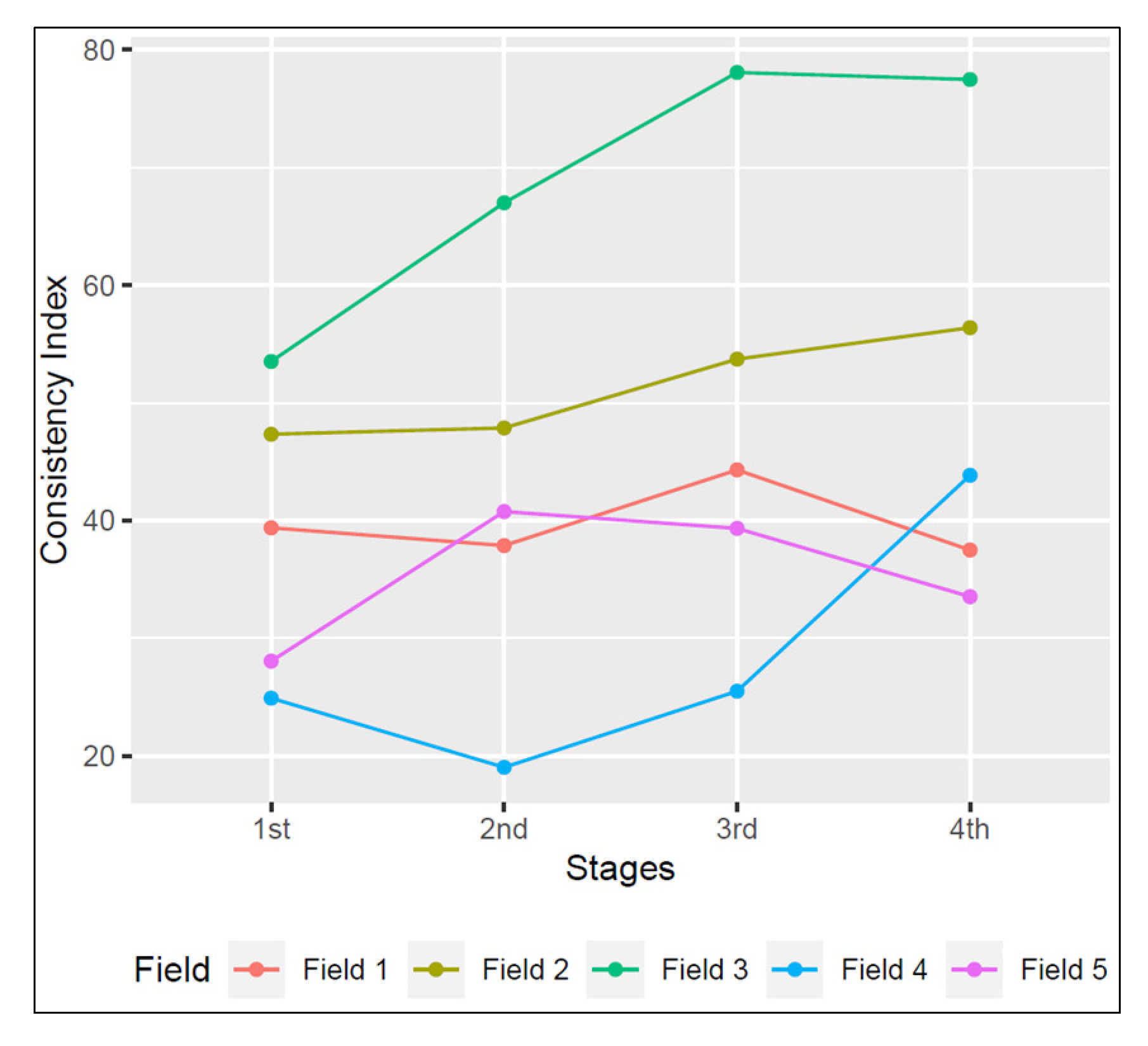
    • Calculate the ‘consistency index’ as the percentage of pixels in the ‘consistently good growth’ or ‘consistently poor growth’ classes. A value of 0 indicates that the maps from each year display different patterns of spatial variation. In contrast, a value of 100 indicates that the maps from each year show identical patterns of spatial variation.
  • Also, for each stage, calculate a map of the multi-year average EVI.
A plot of the consistency index through the season (the result of Step iii b above) was used to investigate whether it can provide information about the likely depths when soil constraints are encountered (which might give rise to an increase in the consistency at the stage of the season when the roots encounter the soil constraints). The proposed interpretations are as follows:
  • If imagery from early in the season shows a consistent pattern (year after year), this might indicate that topsoil constraints, encountered early in the season when roots are shallow, might be causing variation.
  • If imagery from early in the season is not consistent, but imagery from later in the season is, this might indicate that constraints at the depth of roots at that stage of the season (e.g., 60–90 cm for imagery from around 90 days after planting) are causing this increase in consistent patterns.
  • If imagery shows a consistent pattern with increasing consistency through the season, this could indicate the presence of topsoil constraints, which have a lasting impact on growth (even after roots have extended below this depth), or it could indicate the presence of constraints through the profile.
  • If imagery does not show any consistent patterns, this could indicate either no soil constraints are consistently impacting growth, or soil constraints are inconsistently impacting growth (e.g., limiting growth in wet years, beneficial for growth in dry years), or soil constraints are not spatially variable within the field.
This interpretation might back up the interpretations made from correlation analysis (as described in Section 2.4.1, Section 2.4.2, Section 2.4.3).

Appendix A.1. Consistency Index

From the results, we further analyzed the possible approach to indicate the depth of dominant soil constraints based on remote sensing data. We assessed relative growth index consistency within each stage. Figure A1 shows maps for the five fields of the consistently good (green), consistently poor (red) and moderate/inconsistent growth at the four stages of the season. The changes in the resulting consistency index (the percentage of ‘consistent’ pixels in each map) through the season are shown in Figure A2. Our proposed interpretation of Figure A2, in terms of the depth at which soil constraints are encountered in each field, are as follows:
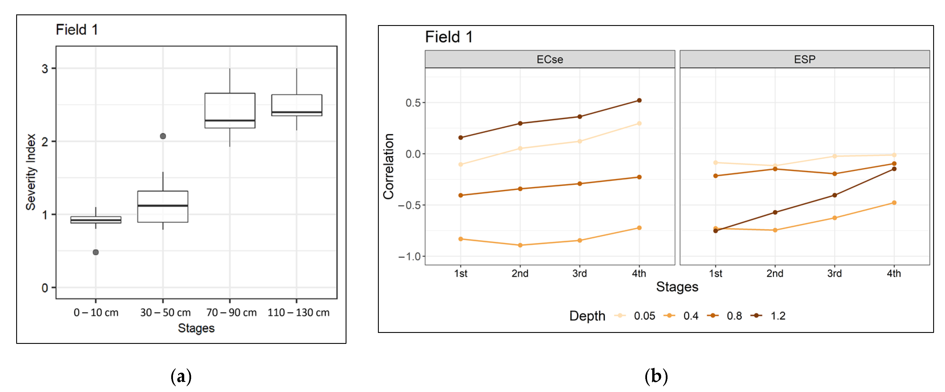
  • Field 1 shows reasonable high consistency from the first stage in the season, with no strong increase later in the season; therefore, topsoil constraints might be important drivers of variation in growth here.
  • Fields 2 and 3 show consistent variation from the first stage in the season, and also a strong increase in consistency throughout the season; therefore, there might be topsoil constraints with a lasting impact or constraints throughout the soil profile here.
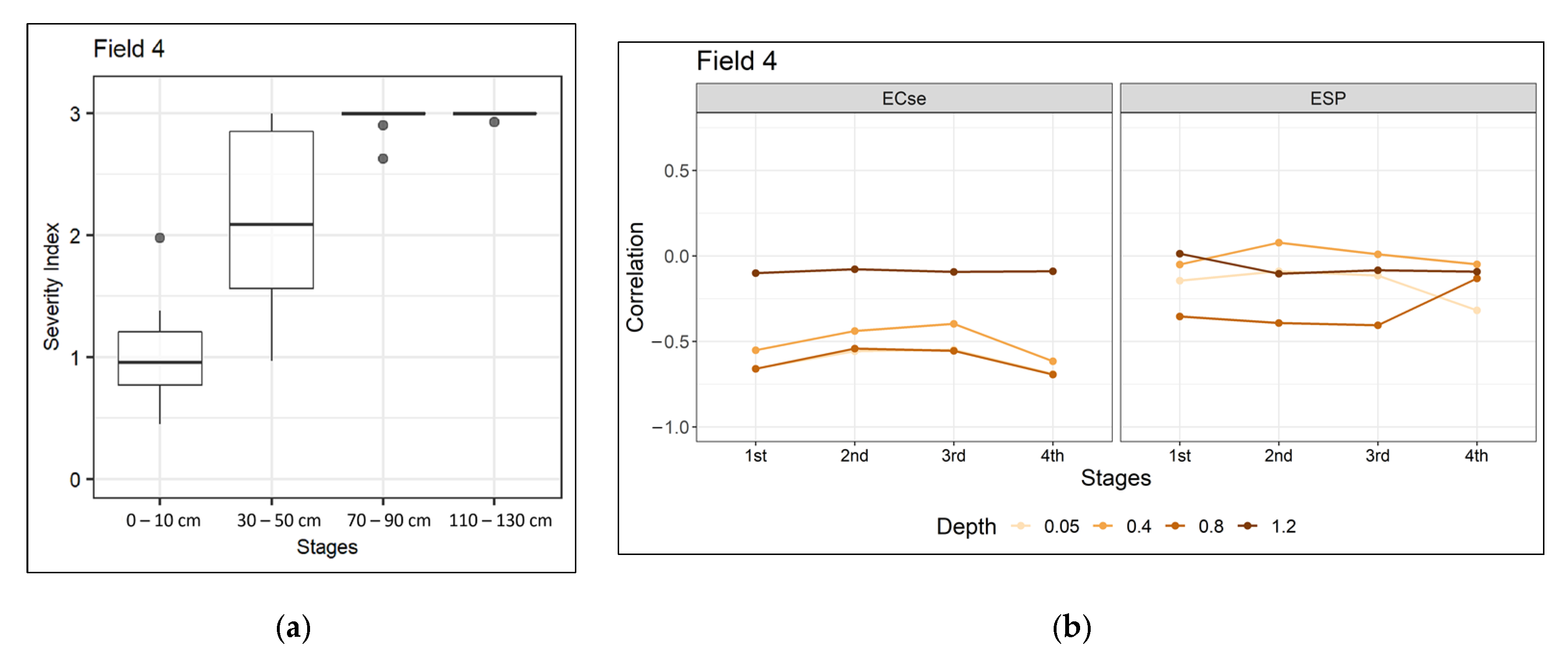
  • Fields 4 and 5 show increases in consistency at the 4th and 2nd stages, respectively, and therefore might be encountering soil constraints at soil depths 90–120 cm and 30–60 cm, respectively.
In the following sections, we group the fields by these interpretations to investigate whether soil data are consistent with these interpretations.
Figure A1. Consistency maps for all five fields. Green = consistently high, red = consistently low, yellow = inconsistent/moderate. Also shown are the soil constraint severity index values for the sampled profiles for the soil depths at which roots might be expected in the four respective stages (0–10 cm, 30–50 cm, 70–90 cm and 110–130 cm, respectively), with red symbols indicating an index of 3 and yellow and index of 0.
Remotesensing 15 03527 g0a1
Figure A2. Consistency index (%) for all five fields.
Remotesensing 15 03527 g0a2

Appendix A.2. Topsoil Issues Indicated by Remote Sensing

For Field 1, the consistency index of around 40% throughout the season (Figure A2) suggested (according to our hypotheses) that topsoil constraints might be an important driver of growth in this field. However, we also found that although the consistency index (percentage of the field classified as ‘consistently good’ or ‘consistently poor’ growth) remained reasonably stable, there were some changes in the spatial variation (Figure A1), with the east side of the field becoming poorer through the season (perhaps encountering subsoil constraints), and the west side consistently poor early in the season (perhaps the effects of topsoil constraints) but becoming less so. The results (Section 3) do not indicate a soil constraint problem at the 0–10 cm depth, whereas at the depth 30–50 cm, which is supported by soil constraints severity variation and correlation with the remote sensing data. While not exactly at the depth indicated by the pattern of the consistency index (reasonably high and constant throughout the season), it is not entirely incompatible since it is still close to the topsoil.

Appendix A.3. Topsoil and Subsoil Issues Indicated by Remote Sensing

Another pattern that can be observed from the consistency analysis is that there are cases with high consistency in the first stage, which continues to increase until the 4th stage. This pattern can be observed in Field 2 and 3 (Figure A1 and Figure A2). For Field 2, the consistency started at 47% and increased to 56%, while for Field 3, the consistency started at 54% and increased to 78%. The maps showing the areas of consistent growth for different stages (Figure A1) show affected areas from early in the season, which expand through the season. The consistent spatial variation early in the season is hypothesized to indicate topsoil constraints, and the later increase in this consistency to indicate the effects of both topsoil and subsoil constraints.
The expectations of topsoil and subsoil issues partly agree with the results analyzed for Field 2 (Section 3). From the results, we found negative correlation between topsoil salinity and 1st stage EVI, which continues to correlate later with the subsoil salinity, even though the problem was not existent for the subsoil. The result gave an indication that the topsoil salinity was the dominant constraint and had an effect on crop growth here throughout the season. Moreover, for Field 3, the expectations of topsoil and subsoil issues were clearly visible for soil sodicity (Section 3).

Appendix A.4. Soil Constraints in Specific Depths Indicated by Remote Sensing

The last pattern from the consistency analysis (Figure A1 and Figure A2) is a jump in consistency percentage at some stage of the season, which suggests (according to our hypotheses) that (i) roots are encountering problems at that stage of the season, and (ii) soil constraints at the expected root depth of that stage might be driving the spatial variation in growth. This case can be observed in Fields 4 and 5. Field 4 showed a jump in the consistency index from the 3rd to the 4th stage, suggesting potential subsoil constraints (at the depth of 90–120 cm, according to the expected root depth at the 4th stage). The jump for Field 4 is also evident from inspection of the maps. For the 4th stage, the large green patch (consistently good growth) appears in the east and red patch appears in the southwest. For Field 5, a jump in consistency can be observed from the 1st to the 2nd stage, suggesting potential soil constraints higher in the profile (30–60 cm according to the expected root depth).
From the result analyzed at Field 4, there was no evidence of soil constraint issues at the depth 110–130 cm (Section 3), yet the correlation between soil salinity and 4th stage EVI does exist at the 70–90 cm depth. This might explain the increase in consistency from the 3rd to the 4th stage (Figure A2); although roots were expected to be at a depth of 90–120 cm at this stage, there is a lot of uncertainty in these root depths and dates (as inferred from the analysis of remote sensing time series data). Encountering soil constraints (subsoil salinity here) at a depth of 70–90 cm between our 3rd and 4th stages (represented by 78–102 and 102–126 days after planting) would not be inconsistent with our interpretation of the increase in consistency at this stage of the season.
For Field 5, the remote sensing analysis showed the increase in consistency between the 1st and 2nd stages suggested the presence of soil constraints at a soil depth of 30–60 cm (represented by our sampled data at 30–50 cm). The results (Section 3) showed soil severity index variation at the 30–60 cm depth, yet there is not enough statistical evidence to backup the indication of soil constraint problems at that depth.

Appendix A.5. Summary

From the results and discussion, we summarize some points for each interpretation. The details are also provided in Table A1.
Table A1. Summary of soil constraint depths, their expected effects on the consistency, and the expected and actual relationships between soil data and EVI.
Feature Description of Remotely Sensed Consistency Index PlotInterpreted
Implication for Soil
Expected Relationships
between Soil Data and EVI
Field Matching Feature Description, and Actual Relationships between Soil Data and EVIStrongest Correlation
between EVI and Soil
Constraints for Field OR
Conclusion from Inspection of Soil–EVI Correlations?
High consistency from the 1st stage onwardsTopsoil constraintsSpatial variation in soil constraint severity index of the topsoil.
Negative correlations of 1st stage EVI with topsoil constraints severity index and with an individual constraint (ECse or ESP).
Field 1
No variation in soil constraint severity index of topsoil.
No correlation between topsoil data (constraint severity index or individual constraints) and 1st stage EVI.
Field 1
30–50 cm soil data (ECse) and 2nd stage EVI.
Partly agrees with expectations from inspection of consistency index plot.
High consistency in the 1st stage then continues to increase until the 4th stageTopsoil and subsoil constraintsSpatial variation in soil constraint severity index at all stages.
Negative correlations of EVI with the severity index and with an individual constraint (ECse or ESP) throughout the profile.
Field 2
Marginal variation in soil constraints severity, yet similar for all the stages.
No correlation between each depth soil constraint severity index and the related stages of EVI.
High negative correlation between topsoil ECse and 1st stage EVI.
Field 2
Strong negative correlation between topsoil ECse not only with the 1st stage but also other stages of EVI.
Partly agrees with expectations from inspection of consistency index plot.
Field 3
Increasing variation from 1st to 4th stage.
Strong negative correlations between EVI and both soil constraints throughout the profile (ECse or ESP).
Field 3
Strong negative correlations between EVI and both soil constraints throughout the profile (ECse or ESP).
Agrees with expectations from inspection of consistency index plot.
A jump in consistency at a certain stage of the seasonConstraints at a certain depthSpatial variation in soil constraint severity index at a certain depth.
Negative correlations of the certain stage EVI with the related depth severity index and with an individual constraint (ECse or ESP).
Field 4 (3rd to 4th stage)
No variation in soil constraint severity index of the 4th stage.
No correlation between 110 and 130 cm soil data (constraint severity index or individual constraints) and 1st stage EVI.
Field 4
70–90 cm soil data (ECse) and 4th stage EVI.
Partly agrees with expectations from inspection of consistency index plot.
Field 5 (1st to 2nd stage)
Soil constraint severity variation does exist in the 2nd stage.
No correlation between 30 and 50 cm soil constraint severity index and 2nd stage EVI.
Insignificant negative correlations between individual constraint (ECse or ESP) at depth 30–50 cm in the 2nd stage.
Field 5
The statistical evidence is not strong enough.
Unclear result.

References

  1. Bot, A.J.; Nachtergaele, F.O.; Young, A. Land Resource Potential and Constraints at Regional and Country Levels; Food and Agriculture Organization of the United Nations: Rome, Italy, 2000. [Google Scholar]
  2. SalCon. Salinity Management Handbook; Queensland Departement of Natural Resources and Mines: Indooroopilly, QLD, Australia, 1997. [Google Scholar]
  3. Orton, T.G.; Mallawaarachchi, T.; Pringle, M.J.; Menzies, N.W.; Dalal, R.C.; Kopittke, P.M.; Searle, R.; Hochman, Z.; Dang, Y.P. Quantifying the economic impact of soil constraints on Australian agriculture: A case-study of wheat. Land Degrad. Dev. 2018, 29, 3866–3875. [Google Scholar] [CrossRef]
  4. Page, K.L.; Dalal, R.C.; Wehr, J.B.; Dang, Y.P.; Kopittke, P.M.; Kirchhof, G.; Fujinuma, R.; Menzies, N.W. Management of the major chemical soil constraints affecting yields in the grain growing region of Queensland and New South Wales, Australia—A review. Soil Res. 2018, 56, 765. [Google Scholar] [CrossRef]
  5. Shaw, R.J. Soil Salinity-Electrical Conductivity and Chloride. In Soil Analysis: An Interpretation Manual; Peverill, K.I., Sparrow, L.A., Reuter, D.J., Eds.; CSIRO Publishing: Clayton, Australia, 1999. [Google Scholar]
  6. Dang, Y.P.; Dalal, R.C.; Routley, R.; Schwenke, G.D.; Daniells, I.G. Subsoil constraints to grain production in the cropping soils of the north-eastern region of Australia: An overview. Aust. J. Exp. Agric. 2006, 46, 19–35. [Google Scholar] [CrossRef] [Green Version]
  7. Dang, Y.P.; Dalal, R.C.; Buck, S.R.; Harms, B.; Kelly, R.; Hochman, Z.; Schwenke, G.D.; Biggs, A.J.W.; Ferguson, N.J.; Norrish, S. Diagnosis, extent, impacts, and management of subsoil constraints in the northern grains cropping region of Australia. Aust. J. Soil Res. 2010, 48, 105–119. [Google Scholar] [CrossRef]
  8. Sheldon, A.R.; Dalal, R.C.; Kirchhof, G.; Kopittke, P.M.; Menzies, N.W. The effect of salinity on plant-available water. Plant Soil 2017, 418, 477–491. [Google Scholar] [CrossRef]
  9. Weil, R.R.; Brady, N.C. The Nature and Properties of Soils, Global Edition, 15th ed.; Pearson Education Limited: London, UK, 2017. [Google Scholar]
  10. Tang, C.; Asseng, S.; Diatloff, E.; Rengel, Z. Modelling yield losses of aluminium-resistant and aluminium-sensitive wheat due to subsurface soil acidity: Effects of rainfall, liming and nitrogen application. Plant Soil. 2003, 254, 349–360. [Google Scholar] [CrossRef]
  11. Li, N.; Arshad, M.; Zhao, D.; Sefton, M.; Triantafilis, J. Determining optimal digital soil mapping components for exchangeable calcium and magnesium across a sugarcane field. Catena 2019, 181, 104054. [Google Scholar] [CrossRef]
  12. Triantafilis, J.; Acácio, F.; Santos, M. Hydrostratigraphic analysis of the Darling River valley (Australia) using electromagnetic induction data and a spatially constrained algorithm for quasi-three-dimensional electrical conductivity imaging. Hydrogeol. J. 2010, 19, 1053. [Google Scholar] [CrossRef]
  13. Zare, E.; Ahmed, M.F.; Malik, R.S.; Subasinghe, R.; Huang, J.; Triantafilis, J. Comparing traditional and digital soil mapping at a district scale using residual maximum likelihood analysis. Soil Res. 2018, 56, 535–547. [Google Scholar] [CrossRef]
  14. Dang, Y.P.; Dalal, R.C.; Mayer, D.G.; McDonald, M.; Routley, R.; Schwenke, G.D.; Buck, S.R.; Daniells, I.G.; Singh, D.K.; Manning, W.; et al. High subsoil chloride concentrations reduce soil water extraction and crop yield on Vertosols in north-eastern Australia. Aust. J. Agric. Res. 2008, 59, 321. [Google Scholar] [CrossRef]
  15. Shukla, M.K.; Lal, R.; Ebinger, M. Principal component analysis for predicting corn biomass and grain yields. Soil Sci. 2004, 169, 215–224. [Google Scholar] [CrossRef]
  16. Rengasamy, P.; Chittleborough, D.; Helyar, K. Root-zone constraints and plant-based solutions for dryland salinity. Plant Soil 2003, 257, 249–260. [Google Scholar] [CrossRef]
  17. Bai, T.; Zhang, N.; Mercatoris, B.; Chen, Y. Jujube yield prediction method combining Landsat 8 vegetation index and the phenological length. Comput. Electron. Agric. 2019, 162, 1011–1027. [Google Scholar] [CrossRef]
  18. Cai, Y.; Guan, K.; Lobell, D.; Potgieter, A.B.; Wang, S.; Peng, J.; Xu, T.; Asseng, S.; Zhang, Y.; You, L.; et al. Integrating satellite and climate data to predict wheat yield in Australia using machine learning approaches. Agric. For. Meteorol. 2019, 274, 144–459. [Google Scholar] [CrossRef]
  19. Dang, Y.P.; Moody, P.W. Quantifying the costs of soil constraints to Australian agriculture: A case study of wheat in north-eastern Australia. Soil Res. 2016, 54, 700–707. [Google Scholar] [CrossRef]
  20. Goodwin, A.W.; Lindsey, L.E.; Harrison, S.K.; Paul, P.A. Estimating wheat yield with normalized difference vegetation index and fractional green canopy cover. Crop. Forage Turfgrass Manag. 2018, 4, 1–6. [Google Scholar] [CrossRef] [Green Version]
  21. Kobayashi, N.; Tani, H.; Wang, X.; Sonobe, R. Crop classification using spectral indices derived from Sentinel-2A imagery. J. Inf. Telecommun. 2020, 4, 67–90. [Google Scholar] [CrossRef]
  22. Lai, Y.R.; Pringle, M.J.; Kopittke, P.M.; Menzies, N.W.; Orton, T.G.; Dang, Y.P. An empirical model for prediction of wheat yield, using time-integrated Landsat NDVI. Int. J. Appl. Earth Obs. Geoinf. 2018, 72, 99–108. [Google Scholar] [CrossRef]
  23. Rouse, J.W.; Hass, R.H.; Schell, J.A.; Deering, D.W. Monitoring vegetation systems in the great plains with ERTS. Third Earth Resour. Technol. Satell. Symp. 1973, 1, 309–317. [Google Scholar]
  24. Semeraro, T.; Mastroleo, G.; Pomes, A.; Luvisi, A.; Gissi, E.; Aretano, R. Modelling fuzzy combination of remote sensing vegetation index for durum wheat crop analysis. Comput. Electron. Agric. 2018, 156, 684–692. [Google Scholar] [CrossRef]
  25. Zhao, Y.; Potgieter, A.B.; Zhang, M.; Wu, B.; Hammer, G.L. Predicting wheat yield at the field scale by combining high-resolution Sentinel-2 satellite imagery and crop modelling. Remote Sens. 2020, 12, 1024. [Google Scholar] [CrossRef] [Green Version]
  26. Huete, A.; Ratana, P.; Didan, K.; Shimabukuro, Y.; Barbosa, H.; Ferreira, L.; Miura, T. Seasonal biophysical dynamics along an amazon eco-climatic gradient using modis vegetation indices. In Proceedings of the Anais XI SBSR, Belo Horizonte, Brazil, 5–10 April 2003. [Google Scholar]
  27. Ulfa, F.; Orton, T.G.; Dang, Y.P.; Menzies, N.W. Are Climate-Dependent Impacts of Soil Constraints on Crop Growth Evident in Remote-Sensing Data? Remote Sens. 2022, 14, 5401. [Google Scholar] [CrossRef]
  28. Ulfa, F.; Orton, T.G.; Dang, Y.P.; Menzies, N.W. A comparison of remote-sensing vegetation indices for assessing within-field variation of wheat yield. In Proceedings of the 20th Agronomy Conference, Toowoomba, QLD, Australia, 18–22 September 2022. [Google Scholar]
  29. Ulfa, F.; Orton, T.G.; Dang, Y.P.; Menzies, N.W. Developing and Testing Remote-Sensing Indices to Represent within-Field Variation of Wheat Yields: Assessment of the Variation Explained by Simple Models. Agronomy 2022, 12, 384. [Google Scholar] [CrossRef]
  30. Dang, Y.P.; Dalal, R.C.; Christopher, J.; Apan, A.A.; Pringle, M.J.; Bailey, K.; Biggs, A.J.W. Advanced Techniques for Managing Subsoil Constraints Project Results Book; Grains Research & Development Corporation: Canberra, Australia, 2010. [Google Scholar]
  31. Dang, Y.P.; Pringle, M.J.; Schmidt, M.; Dalal, R.C.; Apan, A. Identifying the spatial variability of soil constraints using multi-year remote sensing. Field Crops Res. 2011, 123, 248–258. [Google Scholar] [CrossRef]
  32. Dang, Y.P.; Dalal, R.C.; Pringle, M.J.; Biggs, A.J.W.; Darr, S.; Sauer, B.; Moss, J.; Payne, J.; Orange, D. Electromagnetic induction sensing of soil identifies constraints to the crop yields of north-eastern Australia. Soil Res. 2011, 49, 559–571. [Google Scholar] [CrossRef]
  33. Hochman, Z.; Probert, M.; Dalgliesh, N.P. Developing testable hypotheses on the impacts of sub-soil constraints on crops and croplands using the cropping systems simulator APSIM. In Proceedings of the 4th International Crop Science Congress, Brisbane, Australia, 26 September–1 October 2004. [Google Scholar]
  34. Page, K.L.; Dalal, R.C.; Menzies, N.W.; Strong, W.M. Nitrification in a Vertisol subsoil and its relationship to the accumulation of ammonium-nitrogen at depth. Aust. J. Soil Res. 2002, 40, 727–735. [Google Scholar] [CrossRef]
  35. Dang, Y.P.; Routley, R.; McDonald, M.; Dalal, R.C.; Alsemgeest, V.; Orange, D. Effects of chemical subsoil constraints on lower limit of plant available water for crops grown in southwest Queensland. In Proceedings of the 4th International Crop Science Congress, Brisbane, Australia, 26 September–1 October 2004. [Google Scholar]
  36. Thomas, G.A.; Gibson, G.; Nielsen, R.G.H.; Martin, W.D.; Radford, B.J. Effects of tillage, stubble, gypsum, and nitrogen fertiliser on cereal cropping on a red-brown earth in south-west Queensland. Aust. J. Exp. Agric. 1995, 35, 997–1008. [Google Scholar] [CrossRef]
  37. Flood, N.; Danaher, T.; Gill, T.; Gillingham, S. An operational scheme for deriving standardised surface reflectance from landsat TM/ETM+ and SPOT HRG imagery for eastern Australia. Remote Sens. 2013, 5, 83–109. [Google Scholar] [CrossRef] [Green Version]
  38. Zhu, Z.; Wang, S.; Woodcock, C.E. Improvement and expansion of the Fmask algorithm: Cloud, cloud shadow, and snow detection for Landsats 4-7, 8, and Sentinel 2 images. Remote Sens. Environ. 2015, 159, 269–277. [Google Scholar] [CrossRef]
  39. Huete, A.; Didan, K.; Miura, T.; Rodriguez, E.; Gao, X.; Ferreira, L. Overview of the radiometric and biophysical performance of the MODIS vegetation indices. Remote Sens. Environ. 2002, 83, 195–213. [Google Scholar] [CrossRef]
  40. Page, K.L.; Dang, Y.P.; Martinez, C.; Dalal, R.C.; Wehr, J.B.; Kopittke, P.M.; Orton, T.G.; Menzies, N.W. Review of crop-specific tolerance limits to acidity, salinity, and sodicity for seventeen cereal, pulse, and oilseed crops common to rainfed subtropical cropping systems. Land Degrad. Dev. 2021, 32, 2459–2480. [Google Scholar] [CrossRef]
  41. Chong, C.; Bible, B.B.; Ju, H.Y. Germination and emergence. In Handbook of Plant and Crop Physiology, 2nd ed.; NSW Department of Primary Industries: Albury, NSW, Australia, 2001; pp. 57–116. [Google Scholar]
  42. Weaver, J.E. Root habits of wheat. In Root Development of Field Crops; McGraw-Hill Book Company Inc.: New York, NY, USA, 1926. [Google Scholar]
  43. Pozza, L.E.; Filippi, P.; Whelan, B.; Wimalathunge, N.S.; Jones, E.J.; Bishop, T.F.A. Depth to sodicity constraint mapping of the Murray-Darling Basin, Australia. Geoderma 2022, 428, 116181. [Google Scholar] [CrossRef]
  44. Dang, Y.P.; Orton, T.G.; Mcclymont, D.; Menzies, N.W. ConstraintID: A free web-based tool for spatial diagnosis of soil constraints. In Proceedings of the 20th Agronomy Conference, Toowoomba, QLD, Australia, 18–22 September 2022. [Google Scholar]
  45. Orton, T.G.; Mcclymont, D.; Page, K.L.; Menzies, N.W.; Dang, Y.P. ConstraintID: An online software tool to assist grain growers in Australia identify areas affected by soil constraints. Comput. Electron. Agric. 2022, 202, 107422. [Google Scholar] [CrossRef]
Figure 1. The study area in Australia’s northern grains-growing region, and location of the five fields considered in this analysis.
Remotesensing 15 03527 g001
Figure 2. Stages division.
Remotesensing 15 03527 g002
Figure 3. (a) Within-field variation in soil constraint severity in Field 1; (b) correlation between soil constraint and average EVI in Field 1.
Remotesensing 15 03527 g003
Figure 4. (a) Within-field variation in soil constraint severity in Field 2; (b) correlation between soil constraint and average EVI in Field 2.
Remotesensing 15 03527 g004
Figure 5. (a) Within-field variation in soil constraint severity in Field 3; (b) correlation between soil constraint and average EVI in Field 3.
Remotesensing 15 03527 g005
Figure 6. (a) Within-field variation in soil constraint severity in Field 4; (b) correlation between soil constraint and average EVI in Field 4.
Remotesensing 15 03527 g006
Figure 7. (a) Within-field variation in soil constraint severity in Field 5; (b) correlation between soil constraint and average EVI in Field 5.
Remotesensing 15 03527 g007
Table 1. Mean values (min, max) of soil properties and soil constraints severity index for each of the five fields in the study area.
Soil DepthSoil Constraints DataSoil Constraints Severity Index
ECse (dS/m)ESP (%)ECseESPCombined
Field 1
0.050.60 (0.42, 0.79)5.5 (2.9, 6.9)0.20 (0.14, 0.26)0.9 (0.5, 1.1)0.90 (0.48, 1.10)
0.402.19 (1.08, 4.57)15.5 (11.8, 21.4)0.69 (0.36, 1.31)1.2 (0.8, 2.1)1.20 (0.79, 2.07)
0.8010.76 (6.31, 18.76)21.9 (18.7, 27.3)2.28 (1.66, 3.00)2.1 (1.7, 2.4)2.40 (1.92, 3.00)
1.2012.44 (9.20, 21.58)21.7 (16.5, 25.0)2.48 (2.15, 3.00)2.0 (1.3, 2.2)2.50 (2.15, 3.00)
Field 2
0.050.59 (0.41, 1.03)3.5 (1.6, 5.0)0.17 (0.14, 0.23)0.5 (0.3, 0.8)0.50 (0.27, 0.82)
0.401.97 (1.28, 3.18)13.1 (9.9, 17.3)0.63 (0.43, 1.04)0.9 (0.7, 1.3)0.90 (0.66, 1.34)
0.808.13 (4.80, 18.01)22.4 (19.1, 27.4)1.90 (1.36, 3.00)2.1 (1.8, 2.4)2.20 (1.82, 3.00)
1.209.28 (6.62, 12.16)23.7 (20.3, 28.5)2.16 (1.72, 2.52)2.2 (2.0, 2.4)2.30 (2.06, 2.52)
Field 3
0.050.44 (0.31, 0.59)1.1 (0.4, 1.9)0.15 (0.10, 0.20)0.2 (0.1, 0.3)0.20 (0.10, 0.32)
0.400.52 (0.24, 0.76)4.8 (0.6, 11.0)0.17 (0.08, 0.25)0.3 (0.0, 0.7)0.30 (0.08, 0.73)
0.801.19 (0.43, 1.96)10.3 (0.4, 17.4)0.40 (0.14, 0.65)0.7 (0.0, 1.5)0.70 (0.14, 1.48)
1.202.81 (0.58, 5.10)13.9 (0.2, 20.6)0.86 (0.19, 1.42)1.1 (0.0, 2.0)1.20 (0.19, 2.03)
Field 4
0.052.71 (0.40, 7.92)5.8 (2.3, 11.2)0.80 (0.13, 1.98)0.9 (0.4, 1.6)1.00 (0.45, 1.98)
0.4010.43 (1.32, 21.78)16.1 (5.0, 27.9)2.03 (0.44, 3.00)1.3 (0.3, 2.4)2.10 (0.97, 3.00)
0.8020.50 (13.06, 26.38)22.1 (15.3, 28.4)2.95 (2.63, 3.00)2.0 (1.1, 2.4)3.00 (2.63, 3.00)
1.2020.05 (15.46, 23.56)25.2 (17.7, 32.0)2.99 (2.93, 3.00)2.2 (1.5, 2.6)3.00 (2.93, 3.00)
Field 5
0.050.72 (0.34, 1.32)8.2 (3.0, 12.0)0.24 (0.11, 0.44)1.2 (0.5, 1.7)1.20 (0.50, 1.67)
0.402.60 (0.93, 4.43)20.4 (15.0, 28.1)0.83 (0.31, 1.29)1.8 (1.0, 2.4)1.80 (1.00, 2.41)
0.805.67 (3.77, 8.68)29.0 (20.1, 45.8)1.53 (1.15, 2.08)2.4 (2.0, 3.0)2.40 (2.00, 3.00)
1.206.35 (4.78, 8.12)36.5 (25.1, 48.7)1.67 (1.36, 2.01)2.8 (2.3, 3.0)2.80 (2.26, 3.00)
Table 2. Soil constraints’ tolerance limits with severity indices of 0 (no constraint), 1 (potential constraint), 2 (severe constraint) and 3 (extreme constraint).
No Constraint (0)Potential (1)Severe (2)Extreme (3)
ECse0 dS/m3 dS/m8 dS/m16 dS/m
Topsoil ESP0%6%15%30%
Subsoil ESP0%15%20%40%
Table 3. Stages details.
StagesDates Relative to PeakDates Relative to Planting DateExpected Root DepthRepresentative Sampled Depth
1st70–47 days before peak30–53 days after planting30 cm0–10 cm
2nd46–23 days before peak54–77 days after planting60 cm30–50 cm
3rd22 days before peak–2 days after peak78–102 days after planting90 cm70–90 cm
4th3–26 days after peak103–126 days after planting120 cm110–130 cm
Table 4. Correlations between soil constraint severity index for the four sampled soil depths and the EVI from the relevant stage.
Sampled Soil DepthStatisticsField 1Field 2Field 3Field 4Field 5
0–10 cmr−0.10−0.52−0.74−0.13−0.43
p-value0.810.230.010.710.21
30–50 cmr−0.75−0.43−0.67−0.270.00
p-value0.020.330.020.460.97
70–90 cmr−0.25−0.31−0.70−0.32−0.43
p-value0.510.500.010.380.22
110–130 cmr0.570.16−0.720.080.16
p-value0.110.740.010.820.67
Disclaimer/Publisher’s Note: The statements, opinions and data contained in all publications are solely those of the individual author(s) and contributor(s) and not of MDPI and/or the editor(s). MDPI and/or the editor(s) disclaim responsibility for any injury to people or property resulting from any ideas, methods, instructions or products referred to in the content.

