Technical Note

Assessment of Extreme Ocean Winds within Intense Wintertime Windstorms over the North Pacific Using SMAP L-Band Radiometer Observations

V.I. Il’ichev Pacific Oceanological Institute, Far Eastern Branch of the Russian Academy of Sciences, 43 Baltiyskaya, 690041 Vladivostok, Russia
*
Author to whom correspondence should be addressed.
Remote Sens. 2023, 15(21), 5181; https://0-doi-org.brum.beds.ac.uk/10.3390/rs15215181
Submission received: 1 September 2023 / Revised: 20 October 2023 / Accepted: 27 October 2023 / Published: 30 October 2023
(This article belongs to the Special Issue Remote Sensing of Extreme Weather Events: Monitoring and Modeling)

Abstract

:
Here, we examine extreme ocean winds associated with intense wintertime extratropical windstorms over the North Pacific. The study was mainly based on NASA Soil Moisture Active Passive (SMAP) L-band radiometer observations allowing the retrieval of ocean wind speeds up to 70 m/s regardless of precipitation intensity. Additionally, we assessed the ability of atmospheric reanalysis ERA5 and the Climate Forecast System Version 2 (CFSv2) to reproduce high-wind features within severe windstorms, particularly those associated with “explosive” cyclogenesis. The analysis identified 145 windstorm events with hurricane-force (HF) wind zones within the SMAP L-band radiometer swath from 2015 to 2023. These windstorms develop most frequently over two areas: southeast of Kamchatka and south of Alaska, spanning 40–47°N latitudes. Both reanalysis datasets significantly underestimated HF wind speeds compared to SMAP measurements, but CFSv2 tends to reproduce more-intense windstorms than ERA5. Among the notable new findings is that the SMAP data revealed two distinct groups in maximum wind speed distribution, indicating the existence of a separate class of severe windstorm events with a distinct mechanism for extreme wind formation related probably to a Shapiro–Keyser cyclogenesis and the presence of sting jet (SJ) feature. The study highlights the potential of SMAP measurements to study wind extremes and underscores the need for improvements in operational predictive models to better reproduce the formation of SJ windstorms.

Graphical Abstract

1. Introduction

Extratropical cyclones (ETCs) play a critical role in shaping daily weather fluctuations at mid- and high latitudes, frequently leading to exposure to severe winds and waves [1,2,3], storm surges, and intense precipitation [4,5,6], both at sea and along coastlines. These events can have far-reaching socio-economic consequences, impacting shipping routes, maritime infrastructure, and flood-prone regions. Consequently, the measurement of near-surface wind speed becomes one of the major challenges. Notably, a recent investigation [7] demonstrated that a mere 25% rise in peak gust results in a seven-fold amplification of building damage.
Over the last 15–20 years, there has been increased interest in the mechanisms that cause strong winds in extratropical cyclones [8,9,10], and especially sea/land surface gusts [11,12]. Authors have paid special attention to intense windstorms with hurricane-force (HF) winds that generally follow the Shapiro–Keyser (SK) conceptual model [13] and account for the majority of the most-destructive ETCs (in Europe especially) [14,15,16,17]. The published catalog of extratropical cyclones with strong winds [18] makes it possible to systematize knowledge about their structure and evolution and processes influencing surface wind speed enhancement.
Hewson and Neu [9] proposed a wind conceptual model for North Atlantic extratropical cyclones, identifying three distinctive areas: the warm conveyor belt jet (WJ), the cold conveyor belt jet (CJ), and the sting jet (SJ). The latter is the smallest, short-lived, and the most-damaging feature that occurs much less frequently at the end of the bent-back front as high-momentum air descends from the cloud head into a frontal-fracture region [1,19]. The WJ and CJ are low-level jets found in the warm and cold sectors of extratropical cyclones, respectively. These jets can also cause highly destructive surface wind gusts.
One of the primary challenges in studying extreme winds in intense extratropical cyclones is the lack of observational data. Severe windstorms can be brief and localized, making it difficult to capture accurate wind measurements in real-time. Historical records of extreme wind events are often sparse or incomplete, making it challenging to construct long-term datasets of windstorm activity. Additionally, extreme windstorms over the North Atlantic have been studied more extensively than those in the North Pacific—a region producing some of the strongest “bomb cyclones” on Earth [20,21], capable of rapidly amplifying extratropical planetary waves in the Northern Hemisphere [22].
The study of wind characteristics in intense extratropical cyclones is also limited by uncertainties in both forecast models and reanalysis datasets, which are regularly used in the classification and analysis of storm intensity (e.g., [23]). This partly refers to the ability of models to reproduce SJ mesoscale feature causing the short-lived core of HF wind speeds. Difficulties can be associated with both insufficient resolution and boundary layer parametrization issues [9,24]. Concurrently, multi-sensor satellite measurements provide valuable information about atmospheric water vapor and cloud liquid water content, sea surface temperature distribution, and ocean winds. Combining imagery from multiple sensors—operating in both optical and microwave wavelength spectra—can clarify the position, intensity, and stage of development of mesoscale and synoptic-scale weather systems [25,26,27], including extratropical cyclones [28,29,30].
The aim of this study was twofold: to study extreme wind conditions in intense wintertime ETCs revealed over the North Pacific based mainly on the NASA Soil Moisture Active Passive (SMAP) L-band radiometer measurements from 2015 to 2023 and to analyze the possibilities of the fifth-generation atmospheric reanalysis ERA5 and Climate Forecast System Version 2 (CFSv2) datasets to objectively reproduce high wind speed distribution within extratropical windstorms with a focus on those associated with “explosive” cyclogenesis most fully provided by satellite observations. This study consistently developed the first attempt to record sting jet windstorm cases in the North Pacific [31].
Section 2 describes the SMAP measurements, the ERA5 and CFSv2 reanalysis datasets used in the study, as well as the intense windstorm identification method and the intensity metrics. Section 3 presents windstorms’ characteristics and the distribution of extreme ocean wind speeds; additionally, the most-intense windstorm event is analyzed. Finally, a summary and conclusions are given in Section 4.

2. Materials and Methods

2.1. SMAP Observations

The analysis of sea surface wind speed distribution in the extratropical windstorms was carried out by SMAP satellite microwave measurements. The SMAP mission and spacecraft developed at the Jet Propulsion Laboratory (California Institute of Technology, Pasadena, CA, United Sates) with assistance from NASA’s Goddard Spaceflight Center. SMAP was launched in January 2015 into a Sun-synchronous orbit with an L-band radiometer onboard, operating at a frequency of ν = 1.41 GHz. The spatial resolution of the radiometer is about 40 km, and the swath width is 1000 km. In addition to the soil moisture measurement, the SMAP data permit retrievals of ocean surface winds. Daily global fields of the sea surface wind speed retrieved from the radiometer brightness temperatures [32] were taken from the Remote Sensing Systems (California, United Sates) archive with a 0.25 × 0.25 grid. The radiometer onboard SMAP makes it possible to retrieve a sea surface wind speed up to 70 m/s, including in areas of heavy precipitation due to extremely weak scattering and attenuation of electromagnetic waves by individual hydrometeors [33]. We used Version V1.0 of SMAP winds, which takes into account a small dependence of the brightness temperature (Tb) on the ocean surface temperature (SST). This dependence becomes noticeable at mid-latitudes with significant fluctuations in the SST. The study period was limited to the time of the satellite launch and consists of eight cold seasons (November–March) from 2015 to 2023.
We excluded measurements from other satellite sensors—such as the Advanced Scatterometer (European space agency, Paris, France) or the Advanced Microwave Scanning Radiometer 2 (Japan Aerospace Exploration Agency, Tokyo, Japan) —from the analysis because: (1) in scatterometer sensors, the signal saturates when the wind speed reaches 35 m/s [34], and they lose the necessary sensitivity; (2) the signal is attenuated to varying degrees by heavy precipitation, which usually accompanies most HF winds in intense extratropical cyclones. These factors can lead to noticeable errors [35] and misinterpretations of extreme wind speed distributions.

2.2. ERA5 and CFSv2 Reanalysis Datasets

The hourly fields of zonal and meridional wind speed components, air temperature, and sea level atmospheric pressure (SLP) were taken from the ERA5 reanalysis of the European Center for Medium-Range Weather Forecasts (ECMWF, Reading, United Kingdom) [36] and from the operational analysis CFSv2 of the National Forecasting Center The State of the environment of the United States (National Center for Environmental Prediction (NCEP), College Park, Maryland, United States) [37]. The spatial resolution of both datasets is comparable, but the pressure fields obtained from CFSv2 have a coarser grid of 0.5   × 0.5 (see Table 1). In addition, the ERA5 data resolve the lower troposphere at 13 isobaric levels from the sea surface to 500 hPa, providing a higher vertical resolution (200–350 m) and a more-detailed representation of mesoscale wind speed variability compared to CFSv2.

2.3. Windstorms Identification and Their Intensity Metrics

In this study, the ETC was identified as a major windstorm with HF winds and included in the analysis if the following conditions were satisfied:
  • The SMAP-based maximum wind speed was ≥33 m/s (according to the Beaufort scale) within an 800 km radius of the ETC center, which greatly exceeds hurricane-force wind radii determined for North Atlantic hurricanes [38];
  • The ETC low-pressure center was registered over the North Pacific (30–65°N, 130°E–120°W) using hourly SLP fields from ERA5;
  • The selected HF wind zone was within the 1000 km SMAP swath and contained at least four 0.25° × 0.25° grid points, allowing unambiguously determining the maximum wind speed within the entire weather system;
  • Additionally, the distribution of high wind speed was analyzed only for windstorms in which the HF wind area is completely covered by SMAP measurements.
It is important to note that the HF wind zones were associated only with extratropical cyclogenesis (no other causes were observed in the cold seasons of 2015–2023). An exception became the area off the southeastern coast of Kamchatka in March 2017, where SMAP mistakenly measured an extreme wind near drifting ice due to incorrect sea ice masking.
The dataset of identified windstorms was supplemented with SLP values in its centers and geographical coordinates of their position from ERA5 for a period of ±24 h relative to the SMAP measurements time. This made it possible to consider the evolution of the ETCs and identify explosive cyclogenesis events, in which—according to the modified criterion [21]—the following condition is fulfilled:
P c ( t i 6 ) P c ( t i + 6 ) 12   ×   ( s i n 45 s i n φ c ( t i 6 ) + φ c ( t i + 6 ) 2 ) 1 ,
where t i is the time in hours; P c and φ c are the SLP in the windstorm center and the latitude of its position at the times of t i 6 and t i + 6 , respectively. In fact, this formula estimates the rate of the cyclone deepening ( h P a / h ) for 12 h, taking into account the average center position relative to 45°N. Figure 1 shows an event of a severe windstorm over the Northwestern Pacific, which was identified on 25 November 2017 in the field of the SMAP ocean wind speed. The SLP field close in time indicates that the extreme wind area is located in the cyclone’s southwest sector (inset in Figure 1).

2.4. Additional Materials

The images identified the cloudiness structure of the explosive cyclones in the visible or thermal infrared (10–12 μ m) wavelength range obtained by the multi-channel radiometer Advanced Himawari Imager (AHI) with a spatial resolution of 2 km from the Himawari-8 satellite. For the analysis of the dry intrusion into the cyclone central part, the AHI radiometer IR channel at the frequency of 6.9 μ m sensitive to water vapor was used.
Additionally, we used the NOAA Ocean Prediction Center (OPC) HF Low Climatology (https://ocean.weather.gov/climo/storm_track.php, accessed on 12 July 2023) for a comparative analysis of the identified windstorm activity. The OPC dataset contains extratropical storms from 2005 that reached HF wind strength in the North Atlantic and Pacific Oceans. Note that both this dataset and the windstorms we identified do not include ETCs that have undergone an extratropical transition. The express analysis of Japan Meteorological Agency (JMA) best track database (https://www.jma.go.jp/jma/jma-eng/jma-center/rsmc-hp-pub-eg/trackarchives.html, accessed on 12 July 2023) revealed only six extratropical transition events during the 2015–2023 cold seasons (November–March). None of them were included in our study. For more confidence, the synoptic situations analysis and ETCs’ tracking were also carried out by the surface weather and upper air maps of the JMA.

3. Results

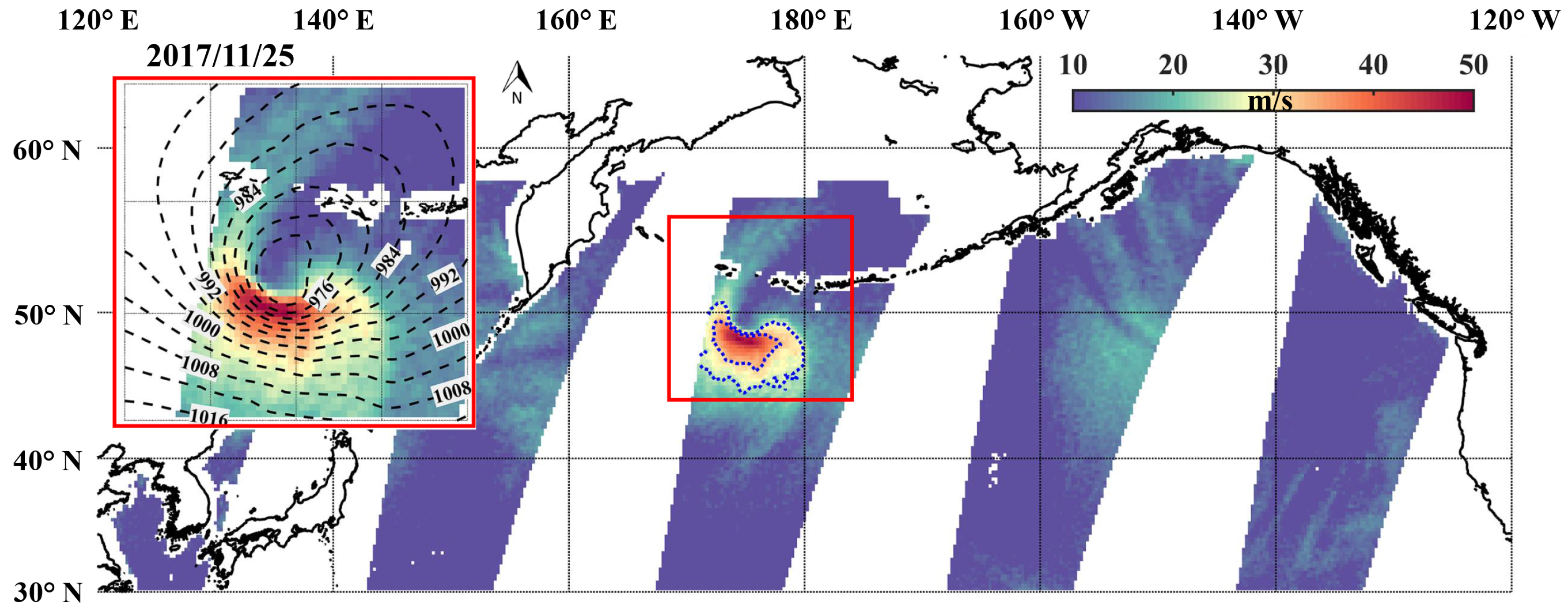
3.1. Windstorms Characteristics

During the eight cold seasons (2015–2023), we registered a total of 145 HF wind events (≥33 m/s) in ETCs within the SMAP swath (hereinafter, windstorms). Figure 2a shows the spatial distribution of windstorms’ centers detected by SMAP and ERA5 data, which is well consistent with the ones derived from the NOAA Ocean Prediction Center archive for the corresponding period and clearly displays major cyclogenesis regions [31]. Although the OPC archive includes a significantly higher number of events with HF wind, the SMAP data statistics are sufficient to represent wintertime windstorm activity in the North Pacific.
Approximately 45% of windstorm events are concentrated southeast from Kamchatka, at the primary region of cyclonic activity in the Northwest Pacific (Figure 2a), where most windstorms were detected [39]. The maximum events were mainly observed during the winter months coinciding with the winter monsoon, with a maximum (37%) in January (inset in Figure 2a). A key factor for cyclogenesis during this period is the advection of a dry cold air mass from the Asian continent. Under favorable conditions, this advection leads to prolonged cold air outbreaks over the Japan and Okhotsk Seas’ surface, as well as the adjacent oceanic areas [40].
The second cyclogenesis area (approximately 20% HF wind events) is located south of Alaska. The analysis of SMAP data revealed that this area is zonally extended along the subpolar oceanic front, spanning latitudes from 40°N to 46°N. Notably, the mechanism responsible for the intensification of cyclones in this region is likely influenced by baroclinic instability, which arises from the unique temperature distribution of the sea surface. Consequently, this distribution causes an elevation in cyclonic potential vorticity within the lower troposphere [41]. It is important to highlight that this local area undergoes a seasonal shift towards the east as sea surface temperature diminishes, resulting in the passing of windstorms ever closer to the west coast of the United States (Figure 2a). Perhaps this is one of the factors in the development of major extratropical windstorms of the Northwest United States [8].
We identified 40% cyclones exhibiting signs of “explosive” development. Of these, 55% were observed in the Kuroshio Extension—a typical area for explosive cyclogenesis in the North Pacific (Figure 2b) [20,21]. Interestingly, the “weak” explosive cyclones by the classification [21] are scattered throughout the North Pacific and reach the United States coast; “strong” ones are located in both local maxima specified in Figure 2a, whereas “super” are concentrated exclusively in the local maximum area to the southeast from Kamchatka (Figure 2b). It should be noted that the distribution of the explosive cyclones range is shifted towards “strong” and “super”, which account for 29% of their total number, compared with 16%, as obtained by the authors [21]. Presumably, this is due to the fact that we selected only HF wind events.

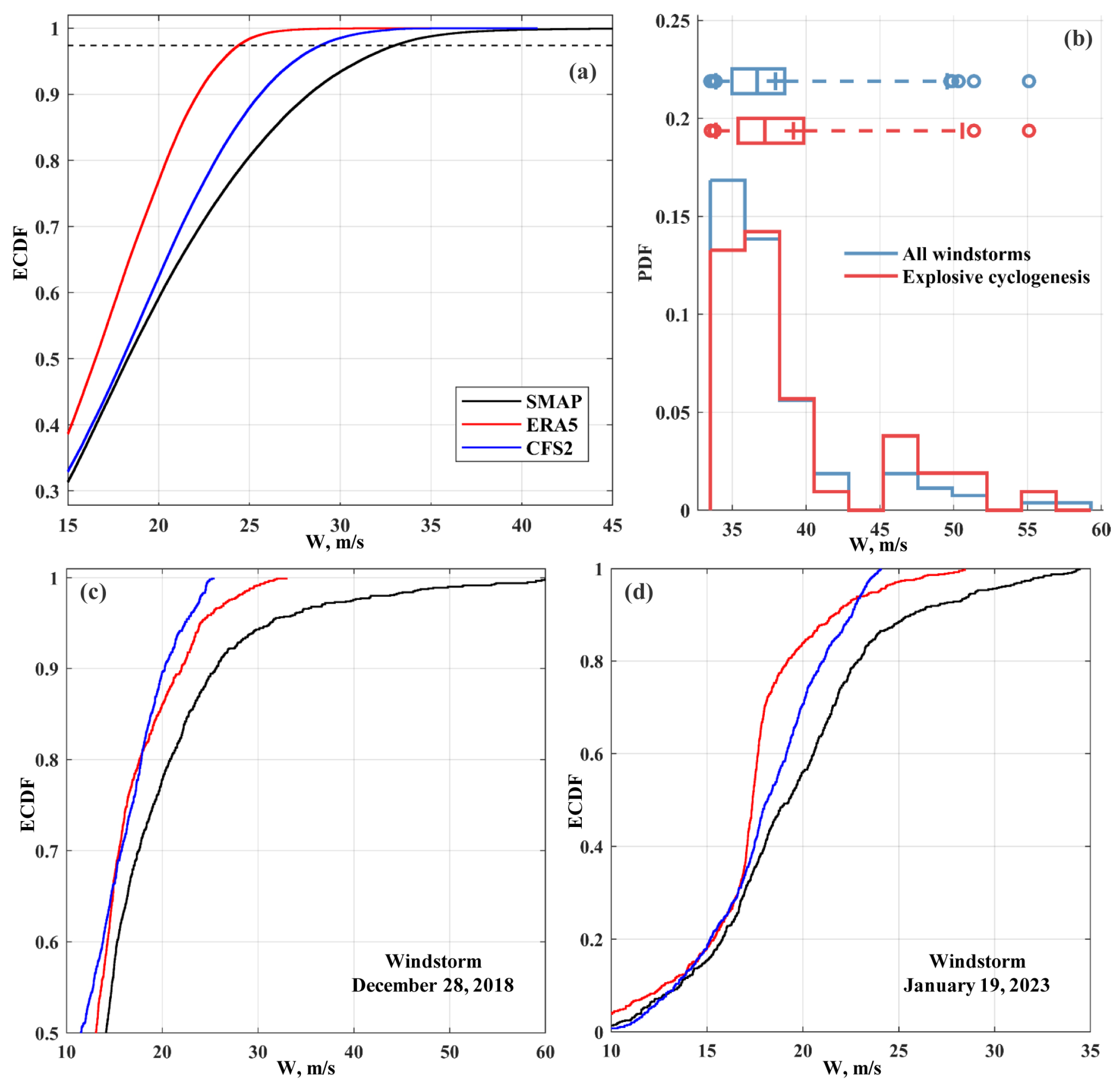
3.2. Distribution of Extreme Ocean Wind Speeds

In order to estimate the distribution of high wind speeds, we compared empirical cumulative distribution functions (ECDFs) of SMAP-based ocean wind speed for 145 identified windstorms to those produced by the ERA5 and CFSv2 datasets (Figure 3a). The ECDFs were firstly constructed for each windstorm within 600 km of its center and then combined. In general, ECDFs of reanalysis datasets exhibit a noticeable underestimation of wind speed (more than 2–3 m/s) in comparison with SMAP observations starting from 15 m/s for ERA5 and 25 m/s for CFSv2. As the value of the wind speed grows, the discrepancy increases rapidly—exceeding 10–15 m/s for both reanalysis datasets at HF winds.
Moreover, there is a discrepancy in the maximum ocean wind speed ( W m a x ) estimates between reanalyses: If CFSv2 recognizes 40% of windstorms with HF winds, the ERA5 identified only three cyclones with W m a x < 38 m/s. Thus, CFSv2 reproduces more-intense cyclones, which agrees with the similar comparison analysis performed for the Atlantic Ocean cyclones identified from 1979 to 2019 [23]. The exception was several windstorm cases (eight windstorms) identified south of 44°N, in which the CFSv2 produces lower HF winds (Figure 3c,d).
The distribution of the W m a x from SMAP exhibits a substantial spread of values with two PDF peaks (Figure 3b), which points to the presence of two different groups. The first group includes the majority of windstorm events with typical values of W m a x = 35–37 m/s; the second group consists of only 13% (14 cases) of the most-intense windstorms with a W m a x ≥ 43 m/s (in some cases, up to 55–60 m/s; see Table 2). Moreover, the second peak noticeably increases for explosive cyclones. Boxplots show (Figure 3b) that, in the W m a x distribution, the first and second modes do not exceed the interquartile range and 95th percentile, respectively.
To strengthen our argument, we applied the Hartigan unimodality test or Hartigan’s dip statistic (HDS) [42], which evaluates the deviation from the unimodality distribution. The calculation of HDS indexes indicated significant (p < 0.05) bimodality in the W m a x PDF for all windstorms and explosive ones. Note that the second PDF peak is not distinguished in the W m a x from the ERA5 and CFSv2 datasets.
We assumed that the second group probably comprises windstorms developed according to the Shapiro–Keyser (SK) conceptual model [13] with the formation of an SJ capable of manifesting itself in the field of surface wind speed. Most of these windstorms (with the exception of two cases; see Table 2) exhibited explosive cyclogenesis 12 h before SMAP measurements. The Himawari-8 imagery of their evolution captured features inherent in SK cyclones: a mutually perpendicular position of the cold and warm fronts (called a T-bone pattern) and the formation of a frontal fracture.
Finally, another interesting feature is related to the geography of the identified severe windstorms with a W m a x ≥ 43 m/s: the centers of 9 out of 14 were located south of the 42nd parallel, while the median position of all 145 cases corresponded to 45°N. Simultaneously, these windstorms have more southerly and zonal storm tracks (at least until the HF wind is observed by SMAP data). This finding is consistent with the requirement of warm moist air to provide the release of conditional symmetric instability [10,43], one of the main physical mechanisms for the development of a sting jet [1,24].

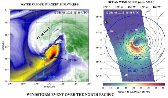
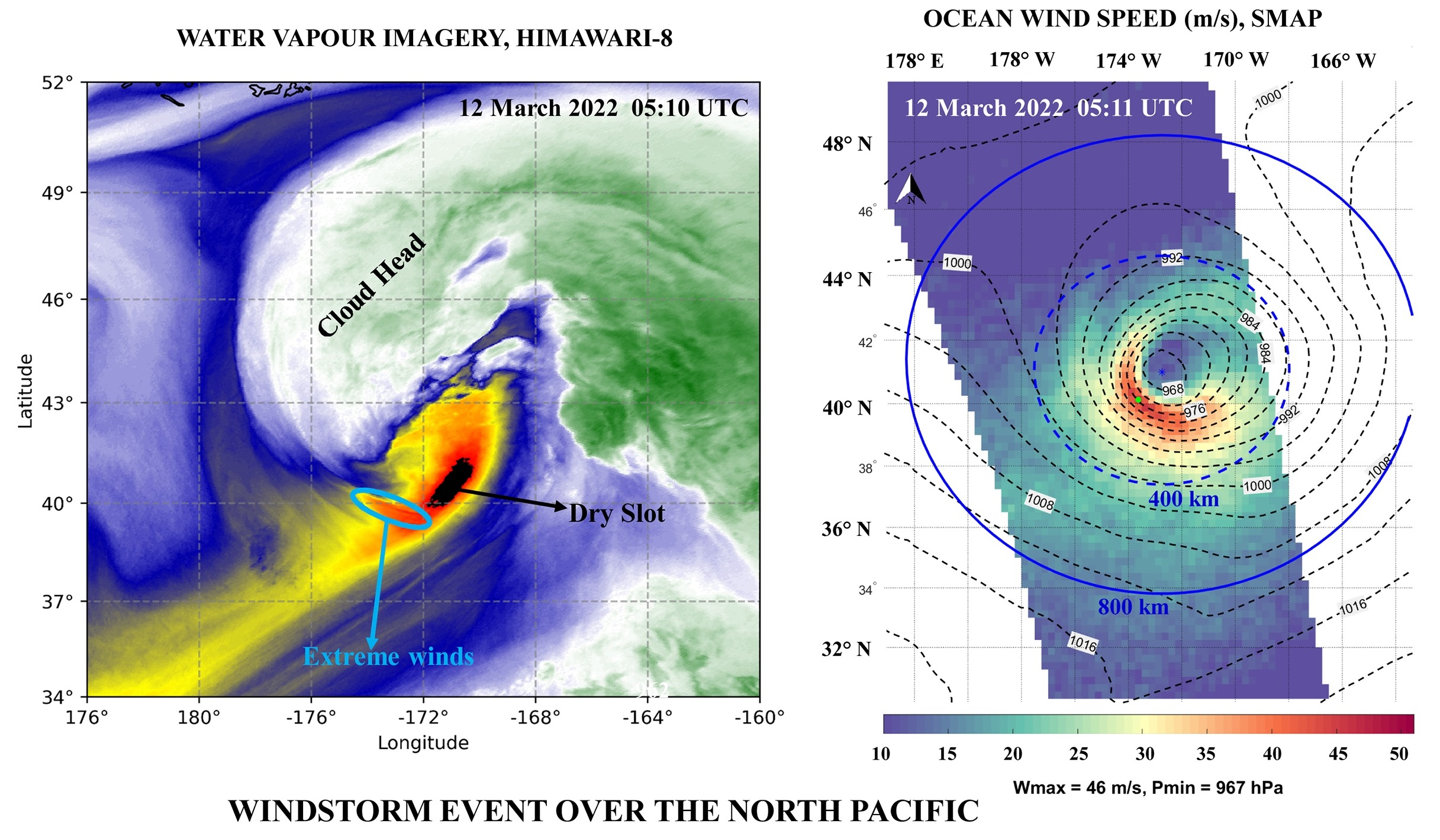
3.3. The Most-Intense Windstorm

This section presents an analysis of the explosive windstorm over the Northwest Pacific with a wind speed of about 60 m/s—the maximum not only for 145 detected cases, but also the previously studied ones over the Atlantic Ocean [44]. The cyclone developed in accordance with the Shapiro—Keyser model, which was shown by such characteristic features as the warm core formation and the mesoscale area with HF winds [13,44].
At the end of December 2018, synoptic conditions contributed to the active cyclogenesis over the North Pacific. The studied cyclone occurred at 18:00 UTC on 27 December in a multicenter cyclonic system under the upper-level frontal zone (surface analysis and AT500 maps JMA (the map of geopotential heights of the 500 hPa isobaric surface); not presented). It quickly moved to the northeast from a relatively warm sea surface to a colder one and intensively deepened. During the day of 28 December, the cyclone deepened from 994 hPa at 00 UTC to 962 hPa at 18 UTC (Figure 4a) with the maximum pressure drop in its center (14 hPa/6 h) between 06:00 and 12:00 UTC (the inset in Figure 4c) and, therefore, classified as “explosive” [31]. For about two days, it was a low baric formation. At 12:00 UTC on 29 December, the cyclonic circulation spread up to the isobaric level of 500 hPa. The trajectory of the cyclone near-surface center made a loop (Figure 4c) when the pressure in its center was minimal and amounted to 944 hPa. Subsequently, the cyclone was moving to the east–northeast and gradually filled.
The tropospheric thermobaric fields’ analysis showed a seclusion process—cutting off and isolating the part of the cyclonic warm sector and, as a result, the warm core forming [13]. The AT500 (Figure 4b) and AT850 (the map of geopotential heights of the 850 hPa isobaric surface isobaric level maps at 12:00 UTC on 28 December and at 00:00 UTC on 29 December JMA demonstrate the tropospheric cold tongue, which was located latitudinally. The meridionally directed heat ridge deviated to the west at about the 50th latitude and skirted the northern periphery of the upper-level low. Thus, the cyclone began to occlude at a distance from its center, and a part of its warm sector was isolating [31].
At 18:00 UTC on 28 December, the cyclone was in an extensive three-center cyclonic system. According to the JMA maps, its horizontal size was about 450 km, and the pressure in the center was 962 hPa (Figure 4a). SMAP registered extreme wind (about 60 m/s) at 19:10 UTC in the cyclone southern sector, when the SLP in its center was 957 hPa by ERA5. The maximum wind speed area was located to the east of the strongest baric gradients zone, in the isobars’ divergence area. This combination of characteristics is considered favorable for SJ formation [9].
IR imagery from Himawari-8 at 15:10, 19:10, and 23:10 UTC on 28 December demonstrated cloud bands separated by dark or translucent stripes (shown by the red arrows in Figure 5a–c). Their presence can be interpreted as an indicator of inclined descending air flows out from the cloud head tip into the frontal area and associated with a dramatic near-surface wind increase [9,44]. The red ellipse in Figure 5b outlines area of high wind speed (≥43 m/s) obtained by SMAP. Another descending sign is the scattering of dense cloudiness on the cloud head “hook” near the cyclone center (green ellipse in the same figures) [9]. It is possible that the wind was increasing up to hurricane force before and after 19:10 UTC. However, the lack of SMAP data does not allow drawing reliable conclusions about the time when its speed was maximum.
One more feature of explosive cyclones is the “dry slot” (marked as DS in Figure 5d–f), i.e., a narrow dry air strip separating the cloud head from the frontal band. A dry slot is associated with a dry intrusion from the stratosphere or upper troposphere and, as a result, with enhancing near-surface wind [44]. In IR images at a frequency of 6.9 μ m (sensitive to the atmosphere water vapor), the DS is identified as a dark area in the brightness fields. Figure 5f shows that the cold air associated with the DS surrounds the cyclone center, secluding the warm air [16,45]. The DS moves to the east–northeast in front of the cyclone center. We can assume that the area of the extreme winds moves in the same direction as the DS.
The wind speed fields by the SMAP and ERA5 data in the area with a radius of 500 km from the cyclone center (outlined by a red dotted line) are shown in Figure 6a–c. This area was determined taking into account the cyclone size and its effect on the wind speed distribution in the environment.
In the SLP field from ERA5, the cyclone center is shifted to the southwest less than 50 km relative to the SMAP estimates (Figure 6a). The cross-section AB passes along the meridian 173.75°E through the area of the extreme winds about 80 km wide, located to south from the center and oriented along the cyclone’s trajectory. Unlike W m a x ≥ 60 m/s by SMAP (Figure 6a), the maximum wind speed by ERA5 (Figure 6b) is about 33 m/s. The analysis of the wind speed difference field by SMAP and ERA5 (Figure 6c) clearly shows small wind speed underestimation by reanalysis (up to about 5 m/s) at wind speeds up to 15 m/s. With wind strengthening, underestimation increases in the cyclone’s southwestern sector. The maximum discrepancy between the SMAP and ERA5 data is registered in the extreme winds area and exceeds 20 m/s.
The comparison of the wind meridional profiles by SMAP and ERA5 data (Figure 6d) also shows a good wind speed agreement up to values of about 23 m/s in the northern quadrant of a windstorm and its systematic underestimation by reanalysis in the southern part. The minimum discrepancies (within the SMAP measurements error) are observed in the cyclone northeastern quadrant (Figure 6d). Finally, the plot demonstrates a dramatic bias in the ERA5 wind speed (more than 25 m/s) for W 30 m/s when compared to the SMAP data.
Cross-sections through the extreme wind area by ERA5 were performed at 16:00 UTC along 41.5°N (Figure 6e) and at 19:00 UTC on 28 December along 42.5°N (Figure 6f). The figures show that ERA5 reproduces descending movement of the extreme wind areas W2 in the troposphere between the isobaric levels of 650 an d850 hPa. The maximum of the vertical wind speed component outlined by the isotach 4 Pa/s, during three hours, moved to east–northeast about 370 km and expanded in the area. At 19:00 UTC, it was determined to be at a height of approximately 2–4 km. The wind field retrieved from ERA5 demonstrated tropospheric jet stream interaction with the strengthening wind in the cyclone. For three hours, the jet stream’s southern periphery descended from the 500 hPa (Figure 6e) to the 600 hPa (Figure 6f) isobaric levels, and W m a x in the cyclone (about 60 m/s) corresponded to the wind speed in the jet stream.
The above-listed totality-specific characteristics of the cyclone development suggest a mesoscale damaging winds process—“sting jet”—the most-dangerous and -destructive feature of explosive cyclogenesis [1,9,13,44].

4. Summary and Conclusions

We presented a comprehensive analysis of wind extremes during wintertime (November–March) extratropical windstorms using SMAP measurements over the North Pacific. The L-band radiometer onboard SMAP allows for the retrieval of sea surface wind speed (W) up to 70 m/s, even in heavy precipitation conditions. In this study, we utilized SMAP data to assess the ability of the fifth-generation atmospheric reanalysis ERA5 and CFSv2 to objectively reproduce severe windstorms, focusing on those associated with “explosive” cyclogenesis and the occurrence of a mesoscale feature probably associated with a sting jet (SJ).
During the period from 2015 to 2023, we identified 145 windstorm events with HF wind zones that fell within the SMAP L-band radiometer swath. Around 43% of these severe windstorms occurred in the southeast of Kamchatka, where explosive cyclones are common in winter due to enhanced baroclinicity caused by cold air outbreaks from eastern Siberia. The second cyclogenesis area is situated to the south of Alaska and extends zonally along the subpolar oceanic front between 40 and 47°N. The intensification of extratropical cyclones in this region may be attributable to enhanced cyclonic potential vorticity in the lower troposphere during autumn–winter, influenced by the regional features of sea surface temperature distribution [41]. The cyclonic activity in this area undergoes a seasonal shift to the east, impacting the evolution of windstorms.
Comparing the maximum wind speed ( W m a x ) distribution obtained from the ERA5 and CFSv2 datasets with that of SMAP measurements, we observed a significant underestimation of extreme wind speeds by both reanalyses. CFSv2 data identify HF winds in only 40% of windstorm events, while ERA5 identifies just three cyclones with a W m a x below 38 m/s. Notably, ERA5 reproduces the descending air flow of the cloud head associated, probably, with the sting jet, despite the discrepancies. Conversely, the SMAP data reveal two distinct groups in the maximum wind speed distribution for all windstorms and explosive ones. The first group consists of the majority of cases with the typical W m a x ranging from 35–37 m/s, while the second group contains only 14% of the most-intense cyclones with W m a x ≥ 43 m/s. These findings suggest the existence of a separate class of severe windstorms exhibiting a distinct mechanism for extreme wind formation.
We hypothesize that these cyclones are developed through the Shapiro—Keyser model of cyclogenesis, leading to the formation of an extreme wind mesoscale area, known as the sting jet. An example of such a severe windstorm, with a wind speed of approximately 60 m/s according to SMAP measurements, represents the highest wind speed among the 145 cases considered. A detailed analysis of this windstorm event demonstrates key features specific to the Shapiro–Keyser model: explosive development without the closure of cold and warm fronts at the cyclone center, the formation of a warm core in the lower troposphere due to seclusion, the appearance of a mesoscale area of extreme wind speeds to the south of the cyclone center, oriented along its trajectory, and the location of the W m a x in the isobars’ divergence area to the east of zone with the strongest baric gradients. These features correspond to the mesoscale sting jet process, which represents the most-dangerous and -destructive aspect of cyclogenesis in the middle latitudes.
This work demonstrated the potential of SMAP measurements in studying wind extremes during wintertime extratropical windstorms over the North Pacific. Our results highlighted the limitations of ERA5 and CFSv2 in reproducing extreme wind speeds compared to SMAP data and emphasize the existence of highly intense extratropical cyclones associated probably with the formation of sting jets over the North Pacific. We understand that the arguments presented here—supporting this significant finding—are not exhaustive and still need further, more-detailed, studies. Improving the realistic reproduction of sting jets requires enhancements in operational predictive models, further underscoring the significance of this study.

Author Contributions

Conceptualization and design of the experiments, M.P. and I.G.; processing and visualization of the satellite data, A.B.; I.G. analyzed the data and wrote the paper; M.P. visualized and analyzed the data and edited and reviewed the paper. All authors have read and agreed to the published version of the manuscript.

Funding

This work was supported by the Russian state budget Theme 121021500054-3 in the development of technology for multi-sensor satellite sensing of atmospheric and oceanic phenomena and by the Federal Science and Technology Program of the Russian Federation (FWMM-2022-0037) in the areas of environmental improvement and climate change for 2021-2030 (FSTP) within the project “Rationale for the Climate Monitoring System of the Far Eastern seas and Development of Methods for Monitoring Extreme Weather and Climate Ocean-Related Phenomena Based on Stationary and Mobile Measuring Complexes, as well as Multi-Sensor Satellite Sensing”.

Data Availability Statement

SMAP ocean wind speed products are available on the Remote Sensing Systems site at https://data.remss.com/smap/wind/L3/v01.0/ (accessed on 12 March 2023). The Himawari-8 gridded data provided by CEReS/Chiba University are on the FTP server: ftp://hmwr829gr.cr.chiba-u.ac.jp (accessed on 12 March 2023). ERA5 and CFSv2 hourly fields can be found at https://cds.climate.copernicus.eu/ (accessed on 23 December 2022) and https://nomads.ncdc.noaa.gov/modeldata/ (accessed on 23 December 2022), respectively. An archive of satellite images and other processed datasets produced by the authors are available upon request.

Acknowledgments

We thank Margarida Belo-Pereira for useful comments and valuable suggestions, which helped to markedly improve our study. This research was supported in part through computational resources provided by the Pacific Oceanological Institute, Vladivostok.

Conflicts of Interest

The authors declare no conflict of interest.

References

  1. Browning, K.A. The sting at the end of the tail: Damaging winds associated with extratropical cyclones. Q. J. R. Meteorol. Soc. 2004, 130, 375–399. [Google Scholar] [CrossRef]
  2. Ponce de León, S.; Guedes Soares, C. Hindcast of extreme sea states in North Atlantic extratropical storms. Ocean Dyn. 2015, 65, 241–254. [Google Scholar] [CrossRef]
  3. Vose, R.S.; Applequist, S.; Bourassa, M.A.; Pryor, S.C.; Barthelmie, R.J.; Blanton, B.; Bromirski, P.D.; Brooks, H.E.; DeGaetano, A.T.; Dole, R.M.; et al. Monitoring and understanding changes in extremes: Extratropical storms, winds, and waves. Bull. Am. Meteorol. Soc. 2014, 95, 377–386. [Google Scholar]
  4. Hawcroft, M.K.; Shaffrey, L.C.; Hodges, K.I.; Dacre, H.F. How much Northern Hemisphere precipitation is associated with extratropical cyclones? Geophys. Res. Lett. 2012, 39, L24809. [Google Scholar] [CrossRef]
  5. Pfahl, S.; Wernli, H. Quantifying the relevance of cyclones for precipitation extremes. J. Clim. 2012, 25, 6770–6780. [Google Scholar] [CrossRef]
  6. Hawcroft, M.; Walsh, E.; Hodges, K.; Zappa, G. Significantly increased extreme precipitation expected in Europe and North America from extratropical cyclones. Environ. Res. Lett. 2018, 13, 124006. [Google Scholar] [CrossRef]
  7. Kezunovic, M.; Dobson, I.; Dong, Y. Impact of extreme weather on power system blackouts and forced outages: New challenges. In Proceedings of the 7th Balkan Power Conference, Sibenik, Croatia, 10–12 September 2008. [Google Scholar]
  8. Mass, C.; Dotson, B. Major Extratropical Cyclones of the Northwest United States: Historical Review, Climatology, and Synoptic Environment. Mon. Weather Rev. 2010, 138, 2499–2527. [Google Scholar] [CrossRef]
  9. Hewson, T.D.; Neu, U. Cyclones, windstorms and the IMILAST project. New Pub Stockh. Uni Press 2015, 6, 81. [Google Scholar] [CrossRef]
  10. Hart, N.C.; Gray, S.L.; Clark, P.A. Sting-Jet Windstorms over the North Atlantic: Climatology and Contribution to Extreme Wind Risk. J. Clim. 2017, 30, 5455–5471. [Google Scholar] [CrossRef]
  11. Manning, C.; Kendon, E.J.; Fowler, H.J.; Roberts, N.M.; Berthou, S.; Suri, D.; Roberts, M.J. Extreme windstorms and sting jets in convection-permitting climate simulations over Europe. Clim. Dyn. 2022, 58, 2387–2404. [Google Scholar] [CrossRef]
  12. Volonté, A.; Gray, S.L.; Clark, P.A.; Martínez-Alvarado, O.; Ackerley, D. Strong surface winds in Storm Eunice. Part 1: Storm overview and indications of sting jet activity from observations and model data. Weather 2023, 9. [Google Scholar] [CrossRef]
  13. Shapiro, M.A.; Keyser, D. Fronts, Jet Streams and the Tropopause. In Extratropical Cyclones: The Erik Palmén Memorial Volume; Newton, C.W., Holopainen, E.O., Eds.; American Meteorological Society: Boston, MA, USA, 1990; pp. 167–191. [Google Scholar] [CrossRef]
  14. Nielsen, N.W.; Sass, B.H. A numerical, high-resolution study of the life cycle of the severe storm over Denmark on 3 December 1999. Tellus A Dyn. Meteorol. Oceanogr. 2003, 55, 338–351. [Google Scholar] [CrossRef]
  15. Wernli, H.; Dirren, S.; Liniger, M.A.; Zillig, M. Dynamical aspects of the life cycle of the winter storm ‘Lothar’ (24–26 December 1999). Q. J. R. Meteorol. Soc. 2002, 128, 405–429. [Google Scholar] [CrossRef]
  16. Pinto, P.; Belo-Pereira, M. Damaging convective and non-convective winds in southwestern Iberia during Windstorm Xola. Atmosphere 2020, 11, 692. [Google Scholar] [CrossRef]
  17. Pinto, P.; Silva, A. The strong wind event of 23rd December 2009 in the Oeste region of Portugal. Rep. Inst. Port. Mar Atmos. 2010, 40. [Google Scholar]
  18. Roberts, J.F.; Champion, A.J.; Dawkins, L.C.; Hodges, K.I.; Shaffrey, L.C.; Stephenson, D.B.; Stringer, M.A.; Thornton, H.E.; Youngman, B.D. The XWS open access catalog of extreme European windstorms from 1979 to 2012. Nat. Hazards Earth Syst. Sci. 2014, 14, 2487–2501. [Google Scholar] [CrossRef]
  19. Schultz, D.M.; Browning, K.A. What is a sting jet? Weather 2017, 72, 63–66. [Google Scholar] [CrossRef]
  20. Iwao, K.; Inatsu, M.; Kimoto, M. Recent changes in explosively developing extratropical cyclones over the winter northwestern Pacific. J. Clim. 2012, 25, 7282–7296. [Google Scholar] [CrossRef]
  21. Zhang, S.; Fu, G.; Lu, C.; Liu, J. Characteristics of Explosive Cyclones over the Northern Pacific. J. Appl. Meteorol. Climatol. 2017, 56, 3187–3210. [Google Scholar] [CrossRef]
  22. Cho, H.O.; Kang, M.J.; Son, S.W.; Hong, D.C.; Kang, J.M. A Critical Role of the North Pacific Bomb Cyclones in the Onset of the 2021 Sudden Stratospheric Warming. Geophys. Res. Lett. 2022, 49, e2022GL099245. [Google Scholar] [CrossRef]
  23. Gramcianinov, C.B.; Campos, R.M.; de Camargo, R.; Hodges, K.I.; Soares, C.G.; da Silva Dias, P.L. Analysis of Atlantic extratropical storm tracks characteristics in 41 years of ERA5 and CFSR/CFSv2 databases. Ocean Eng. 2020, 216, 108111. [Google Scholar] [CrossRef]
  24. Clark, P.; Browning, K.; Wang, C. The sting at the end of the tail: Model diagnostics of fine-scale three-dimensional structure of the cloud head. Q. J. R. Meteorol. Soc. A J. Atmos. Sci. Appl. Meteorol. Phys. Oceanogr. 2005, 131, 2263–2292. [Google Scholar] [CrossRef]
  25. Pichugin, M.K.; Gurvich, I.A.; Zabolotskikh, E.V. Severe Marine Weather Systems During Freeze-Up in the Chukchi Sea: Cold-Air Outbreak and Mesocyclone Case Studies From Satellite Multisensor Measurements and Reanalysis Datasets. IEEE J. Sel. Top. Appl. Earth Obs. Remote Sens. 2019, 12, 3208–3218. [Google Scholar] [CrossRef]
  26. Gurvich, I.; Pichugin, M.; Baranyuk, A. Satellite Multi-Sensor Data Analysis of Unusually Strong Polar Lows over the Chukchi and Beaufort Seas in October 2017. Remote Sens. 2023, 15, 120. [Google Scholar] [CrossRef]
  27. Zabolotskikh, E.V.; Gurvich, I.A.; Chapron, B. Polar lows over the Eastern part of the Eurasian Arctic: The sea-ice retreat consequence. IEEE Geosci. Remote Sens. Lett. 2016, 13, 1492–1496. [Google Scholar] [CrossRef]
  28. Mitnik, L.M.; Mitnik, M.L.; Gurvich, I.A.; Vykochko, A.V.; Pichugin, M.K.; Cherny, I.V. Water vapor, cloud liquid water content and wind speed in tropical, extratropical and polar cyclones over the Northwest Pacific Ocean. In Proceedings of the 2012 IEEE International Geoscience and Remote Sensing Symposium, Munich, Germany, 22–27 July 2012; pp. 1940–1943. [Google Scholar]
  29. Vasilyeva, P.V.; Zabolotskikh, E.V.; Chapron, B. Comparative analysis of the North Atlantic and North Pacific extratropical cyclone characteristics retrieved from ERA-Interim reanalysis and AMSR-E data. Curr. Probl. Remote Sens. Earth Space 2018, 15, 236–248. (In Russian) [Google Scholar] [CrossRef]
  30. Mitnik, L.; Baranyuk, A.; Kuleshov, V.; Mitnik, M. Bomb Cyclones over the North Pacific: Atmospheric Structure and Parameters According to Passive and Active Microwave Measurements from Space. Russ. Meteorol. Hydrol. 2023, 48, 10–19. [Google Scholar] [CrossRef]
  31. Pichugin, M.; Gurvich, I.; Baranyuk, A. Analysis of extreme winds in intense extratropical cyclones over the North Pacific based on satellite observations from SMAP. Curr. Probl. Remote Sens. Earth Space 2022, 19, 287–299. (In Russian) [Google Scholar] [CrossRef]
  32. Meissner, T.; Ricciardulli, L.; Wentz, F.J. Capability of the SMAP Mission to Measure Ocean Surface Winds in Storms. Bull. Am. Meteorol. Soc. 2017, 98, 1660–1677. [Google Scholar] [CrossRef]
  33. Meissner, T.; Ricciardulli, L.; Manaster, A. Tropical cyclone wind speeds from WindSat, AMSR and SMAP: Algorithm development and testing. Remote Sens. 2021, 13, 1641. [Google Scholar] [CrossRef]
  34. Donelan, M.; Haus, B.K.; Reul, N.; Plant, W.; Stiassnie, M.; Graber, H.; Brown, O.B.; Saltzman, E. On the limiting aerodynamic roughness of the ocean in very strong winds. Geophys. Res. Lett. 2004, 31, L18306. [Google Scholar] [CrossRef]
  35. Bourassa, M.A.; Meissner, T.; Cerovecki, I.; Chang, P.S.; Dong, X.; De Chiara, G.; Donlon, C.; Dukhovskoy, D.S.; Elya, J.; Fore, A.; et al. Remotely sensed winds and wind stresses for marine forecasting and ocean modeling. Front. Mar. Sci. 2019, 6, 443. [Google Scholar] [CrossRef]
  36. Hersbach, H.; Bell, B.; Berrisford, P.; Hirahara, S.; Horányi, A.; Muñoz-Sabater, J.; Nicolas, J.; Peubey, C.; Radu, R.; Schepers, D.; et al. The ERA5 global reanalysis. Q. J. R. Meteorol. Soc. 2020, 146, 1999–2049. [Google Scholar] [CrossRef]
  37. Saha, S.; Moorthi, S.; Wu, X.; Wang, J.; Nadiga, S.; Tripp, P.; Behringer, D.; Hou, Y.T.; Chuang, H.-Y.; Iredell, M.; et al. The NCEP Climate Forecast System Version 2. J. Clim. 2014, 27, 2185–2208. [Google Scholar] [CrossRef]
  38. Bell, K.; Ray, P.S. North Atlantic hurricanes 1977–1999: Surface hurricane-force wind radii. Mon. Weather Rev. 2004, 132, 1167–1189. [Google Scholar] [CrossRef]
  39. Gyakum, J.R.; Anderson, J.R.; Grumm, R.H.; Gruner, E.L. North Pacific Cold-Season Surface Cyclone Activity: 1975–1983. Mon. Weather Rev. 1989, 117, 1141–1155. [Google Scholar] [CrossRef]
  40. Fletcher, J.; Mason, S.; Jakob, C. The climatology, meteorology, and boundary layer structure of marine cold air outbreaks in both hemispheres. J. Clim. 2016, 29, 1999–2014. [Google Scholar] [CrossRef]
  41. Pickart, R.S.; Macdonald, A.M.; Moore, G.W.K.; Renfrew, I.A.; Walsh, J.E.; Kessler, W.S. Seasonal Evolution of Aleutian Low Pressure Systems: Implications for the North Pacific Subpolar Circulation. J. Phys. Oceanogr. 2009, 39, 1317–1339. [Google Scholar] [CrossRef]
  42. Hartigan, J.A.; Hartigan, P.M. The dip test of unimodality. Ann. Stat. 1985, 13, 70–84. [Google Scholar] [CrossRef]
  43. Martínez-Alvarado, O.; Gray, S.L.; Catto, J.L.; Clark, P.A. Sting jets in intense winter North-Atlantic windstorms. Environ. Res. Lett. 2012, 7, 024014. [Google Scholar] [CrossRef]
  44. Clark, P.A.; Gray, S.L. Sting jets in extratropical cyclones: A review. Q. J. R. Meteorol. Soc. 2018, 144, 943–969. [Google Scholar] [CrossRef]
  45. Browning, K. The dry intrusion perspective of extra-tropical cyclone development. Meteorol. Appl. 1997, 4, 317–324. [Google Scholar] [CrossRef]
Figure 1. Example of the severe windstorm event (which is contoured by the red square) detected on 25 November 2017 in the field of near-sea surface wind speed (color scale in m/s) retrieved from SMAP measurements. The isotachs 25 and 33 m/s are outlined in blue. The inset in the upper right corner shows the enlarged fragment of SMAP-based wind speed with SLP isobars from the ERA5 dataset.
Remotesensing 15 05181 g001
Figure 2. The frequency map of extratropical cyclones with HF wind events (a); the map of explosive cyclogenesis activity with different intensity (“Weak”, “Moderate”, “Strong”, and “Super”) by classification [21] (b). The maps are constructed for the eight cold seasons (November–March) of 2015–2023 by SMAP data. The color scale in (a); in events per unit area of 10 6 km2 (corresponding to a spherical segment of 5 ). The inset in (a) shows the seasonal distribution of windstorm events. In the lower-left corner in (b) is presented a scale in kilometers and land miles.
Remotesensing 15 05181 g002
Figure 3. Distribution of high ocean wind speed (W) within windstorms area: comparison of W empirical cumulative distribution functions (ECDFs) between SMAP data (black lines), ERA5 (red lines), and CFSv2 (blue lines) datasets, produced for identified windstorms (a) and ones on 28 December 2018 (c) and 19 January 2023 (d); (b) the maximum wind speed ( W m a x , m/s) probability density function and box and whiskers plots (circles denote events with more/less than the 95th/5th percentile of W m a x ) in windstorms with non-explosive (blue line) and explosive (red line) cyclogenesis. The black dotted line in (a) refers to the ECDF, where SMAP-based W = 33 m/s.
Remotesensing 15 05181 g003
Figure 4. The maps from the JMA of surface analysis at 18 UTC (a) and AT500 at 12 UTC (b) on 28 December 2018; IR image obtained by the AHI radiometer onboard Himawari-8 satellite at 19:00 UTC on 28 December and cyclone trajectory (blue/red) from 18:00 UTC on 27 December 2018 to 12:00 UTC on 1 January 2019 by the JMA (c). The inset in (c) is the pressure evolution graph in the cyclone center. The red lines on the trajectory and graph indicate the explosive cyclogenesis.
Remotesensing 15 05181 g004
Figure 5. Infrared images at the wavelengths of 10.8 μ m (ac) and 6.9 μ m (df) obtained by the AHI radiometer from the Himawari-8 satellite at 15:10 (a,d), 19:10 (b,e), and 23:10 (c,f) UTC on 28 December 2018. The sign “X” indicates the cyclone center. Red arrows indicate dark gaps between the cloud bands. The red ellipse in (b) outlines the extreme wind area. Green ellipses in (ac) indicate areas of dense clouds scattering at the cloud head end. “DS” in (df) denotes the “dry slot” area.
Remotesensing 15 05181 g005
Figure 6. The combined fields of the near-sea surface wind speed by the SMAP measurements at 19:10 UTC with sea level atmospheric pressure from ERA5 at 19:00 UTC on 28 December 2018 (a), the wind speed fields from ERA5 (b), and the wind speed difference field between SMAP observations and ERA5 data (c) within an area with a radius of 500 km (outlined by a red dotted line); the plot of wind speed along the line AB by ERA5 (solid line) and SMAP (dashed line) (d); zonal cross-sections of the horizontal (in m/s) and vertical (in Pa/s) wind speed components from ERA5 constructed through local maxima of 850 hPa wind speed at 16:00 UTC (e) and 19:00 UTC (f). The line AB runs along the meridian 73.75°E. Scales in (ac) are in m/s. W1 and W2 in (e,f) are the extreme wind local areas. The triangle in (e,f) indicates the longitude of the cyclone center position.
Remotesensing 15 05181 g006
Table 1. Main characteristics of reanalysis datasets.
CharacteristicsERA-5 (ECMWF)CFSv2 (NCEP)
PeriodFrom 1979 to present timeFrom 2011 to present time
Temporary resolutionHourlyHourly
Model resolutionT639, 31 km27 km
Horizontal resolution0.25   × 0.25 0.2   × 0.2 , 0.5 × 0.5
Vertical resolution137 levels (0.01 hPa)37 levels (1 hPa)
Data assimilation4D-Var3D-Var
Table 2. Characteristics of the most-intense windstorms with extreme winds from SMAP (≥43 m/s). The minimum SLP at the windstorm center was obtained from the ERA5 dataset. The * symbol indicates non-explosive cyclones.
DateTime (UTC)Pc (hPa)Lon.Lat.Wmax (m/s)Intensity (hPa/h)
12 December 201519:10936176.048.8462.14
14 January 201604:36949191.840.0501.22
9 January 201720:27962153.038.5490.76 *
25 November 201718:45970175.050.0502.32
6 January 201820:01968162.837.3452.07
28 December 201819:11957173.343.5602.34
11 March 201907:51962144.038.8502.24
27 December 201920:01957159.337.8471.33
29 December 202018:21971179.037.3552.01
31 December 202006:03928168.048.0472.61
8 January 202104:23965197.341.3512.04
20 January 202106:50974164.343.3470.70 *
12 March 202205:10967187.241.0461.86
29 November 202205:23966176.238.5431.02
Disclaimer/Publisher’s Note: The statements, opinions and data contained in all publications are solely those of the individual author(s) and contributor(s) and not of MDPI and/or the editor(s). MDPI and/or the editor(s) disclaim responsibility for any injury to people or property resulting from any ideas, methods, instructions or products referred to in the content.

