
3D-ResNet-BiLSTM Model: A Deep Learning Model for County-Level Soybean Yield Prediction with Time-Series Sentinel-1, Sentinel-2 Imagery, and Daymet Data


Abstract
:1. Introduction
2. Materials and Methods
2.1. Study Area
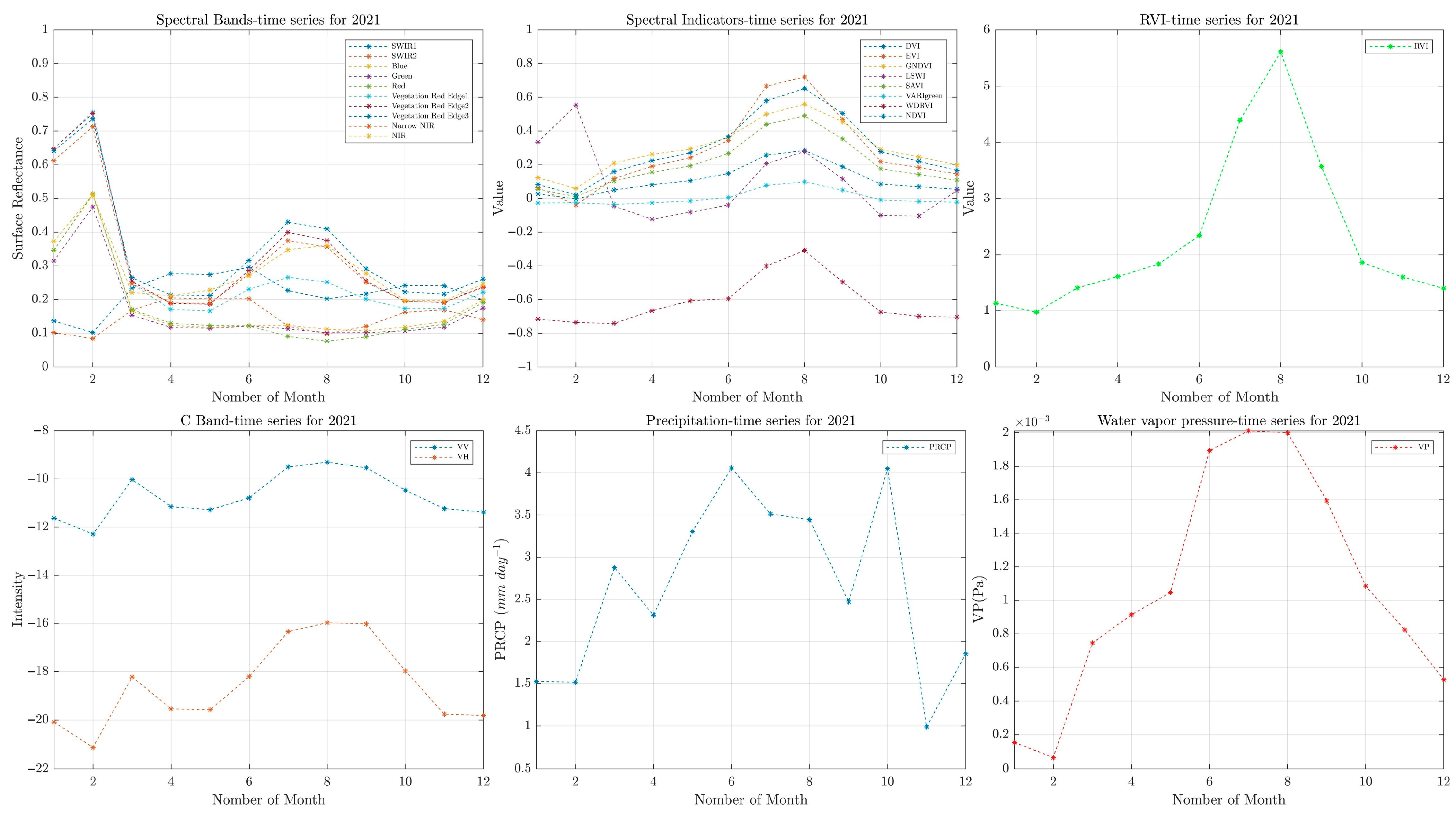
2.2. Dataset
2.3. Methodology
2.3.1. Feature Selection
2.3.2. 3D-ResNet-BiLSTM Model Architecture
3D-ResNet Component
Bi-LSTM Component
2.4. Evaluation Metrics
3. Experimental Results
3.1. Experimental Setup
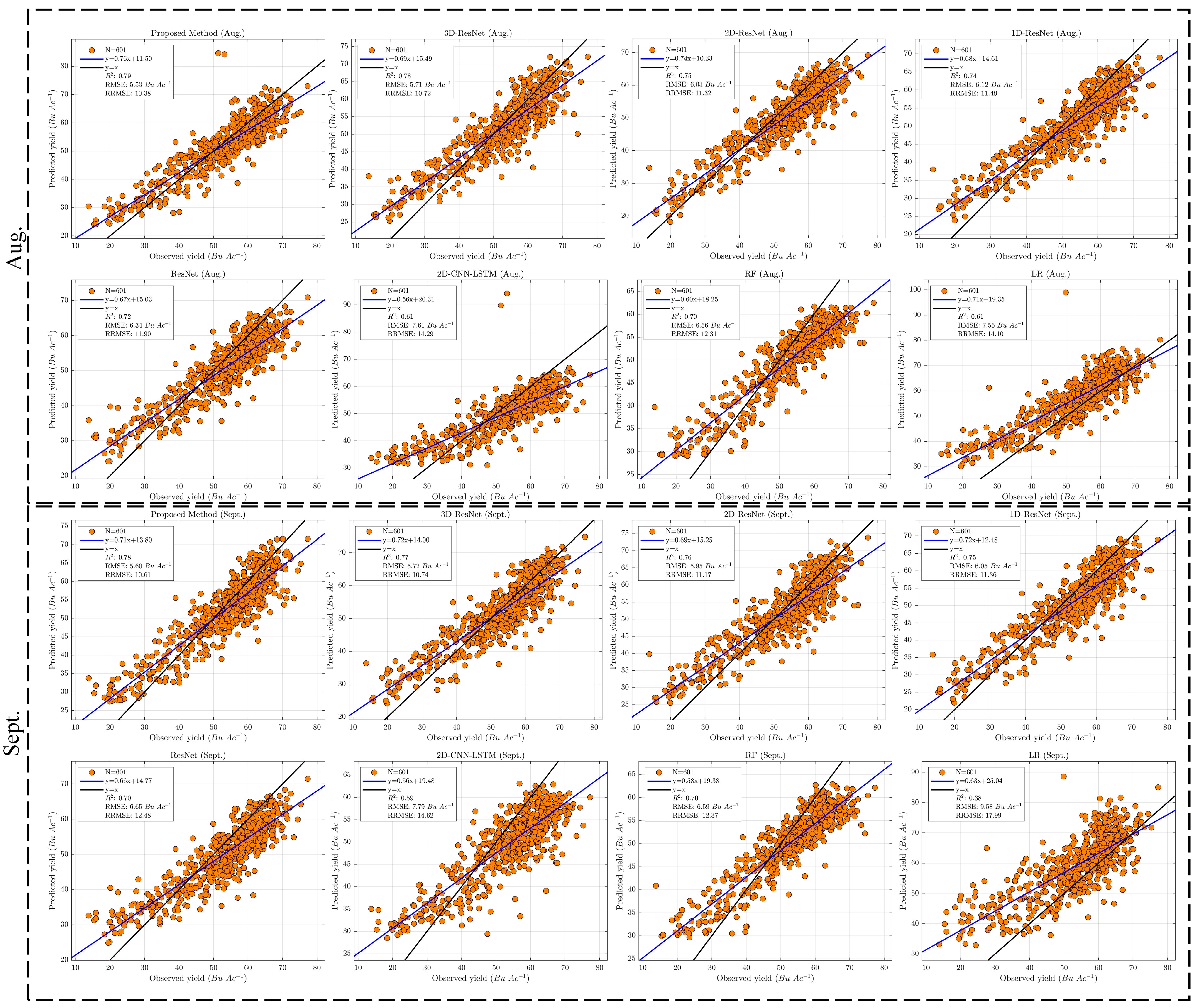
3.2. Comparative Results of the Soybean Yield Prediction
4. Discussion
5. Conclusions
Author Contributions
Funding
Data Availability Statement
Acknowledgments
Conflicts of Interest
References
- Mohite, J.; Sawant, S.; Pandit, A.; Agrawal, R.; Pappula, S. Soybean Crop Yield Prediction by Integration of Remote Sensing and Weather Observations. Int. Arch. Photogramm. Remote Sens. Spat. Inf. Sci. 2023, 48, 197–202. [Google Scholar] [CrossRef]
- Fathi, M.; Shah-Hosseini, R.; Moghimi, A. Comparison of Some Deep Neural Networks for Corn and Soybean Mapping in Iowa State using Landsat imagery. Earth Obs. Geomat. Eng. 2022, 6, 57–66. [Google Scholar]
- Bharadiya, J.P.; Tzenios, N.T.; Reddy, M. Forecasting crop yield using remote sensing data, rural factors, and machine learning approaches. J. Eng. Res. Rep. 2023, 24, 29–44. [Google Scholar]
- Muruganantham, P.; Wibowo, S.; Grandhi, S.; Samrat, N.H.; Islam, N. A systematic literature review on crop yield prediction with deep learning and remote sensing. Remote Sens. 2022, 14, 1990. [Google Scholar] [CrossRef]
- Sun, J.; Di, L.; Sun, Z.; Shen, Y.; Lai, Z. County-level soybean yield prediction using deep CNN-LSTM model. Sensors 2019, 19, 4363. [Google Scholar] [CrossRef] [PubMed]
- Rashid, M.; Bari, B.S.; Yusup, Y.; Kamaruddin, M.A.; Khan, N. A comprehensive review of crop yield prediction using machine learning approaches with special emphasis on palm oil yield prediction. IEEE Access 2021, 9, 63406–63439. [Google Scholar] [CrossRef]
- Qiao, M.; He, X.; Cheng, X.; Li, P.; Luo, H.; Zhang, L.; Tian, Z. Crop yield prediction from multi-spectral, multi-temporal remotely sensed imagery using recurrent 3D convolutional neural networks. Int. J. Appl. Earth Obs. Geoinf. 2021, 102, 102436. [Google Scholar] [CrossRef]
- Zhou, S.; Xu, L.; Chen, N. Rice Yield Prediction in Hubei Province Based on Deep Learning and the Effect of Spatial Heterogeneity. Remote Sens. 2023, 15, 1361. [Google Scholar] [CrossRef]
- Sun, J.; Lai, Z.; Di, L.; Sun, Z.; Tao, J.; Shen, Y. Multilevel deep learning network for county-level corn yield estimation in the us corn belt. IEEE J. Sel. Top. Appl. Earth Obs. Remote Sens. 2020, 13, 5048–5060. [Google Scholar] [CrossRef]
- Huang, H.; Huang, J.; Feng, Q.; Liu, J.; Li, X.; Wang, X.; Niu, Q. Developing a dual-stream deep-learning neural network model for improving county-level winter wheat yield estimates in China. Remote Sens. 2022, 14, 5280. [Google Scholar] [CrossRef]
- Van Klompenburg, T.; Kassahun, A.; Catal, C. Crop yield prediction using machine learning: A systematic literature review. Comput. Electron. Agric. 2020, 177, 105709. [Google Scholar] [CrossRef]
- Pang, A.; Chang, M.W.; Chen, Y. Evaluation of random forests (RF) for regional and local-scale wheat yield prediction in southeast Australia. Sensors 2022, 22, 717. [Google Scholar] [CrossRef] [PubMed]
- Li, Z.; Chen, Z.; Cheng, Q.; Duan, F.; Sui, R.; Huang, X.; Xu, H. UAV-based hyperspectral and ensemble machine learning for predicting yield in winter wheat. Agronomy 2022, 12, 202. [Google Scholar] [CrossRef]
- Guo, Y.; Fu, Y.; Hao, F.; Zhang, X.; Wu, W.; Jin, X.; Bryant, C.R.; Senthilnath, J. Integrated phenology and climate in rice yields prediction using machine learning methods. Ecol. Indic. 2021, 120, 106935. [Google Scholar] [CrossRef]
- Khankeshizadeh, E.; Mohammadzadeh, A.; Moghimi, A.; Mohsenifar, A. FCD-R2U-net: Forest change detection in bi-temporal satellite images using the recurrent residual-based U-net. Earth Sci. Inform. 2022, 15, 2335–2347. [Google Scholar] [CrossRef]
- You, J.; Li, X.; Low, M.; Lobell, D.; Ermon, S. Deep Gaussian process for crop yield prediction based on remote sensing data. In Proceedings of the AAAI Conference on Artificial Intelligence, San Francisco, CA, USA, 4–9 February 2017. [Google Scholar]
- Terliksiz, A.S.; Altýlar, D.T. Use of deep neural networks for crop yield prediction: A case study of soybean yield in Lauderdale county, alabama, USA. In Proceedings of the 2019 8th International Conference on Agro-Geoinformatics (Agro-Geoinformatics), Istanbul, Turkey, 16–19 July 2019; pp. 1–4. [Google Scholar]
- Khaki, S.; Wang, L.; Archontoulis, S.V. A cnn-rnn framework for crop yield prediction. Front. Plant Sci. 2020, 10, 1750. [Google Scholar] [CrossRef]
- Khaki, S.; Pham, H.; Wang, L. Simultaneous corn and soybean yield prediction from remote sensing data using deep transfer learning. Sci. Rep. 2021, 11, 11132. [Google Scholar] [CrossRef]
- Schwalbert, R.A.; Amado, T.; Corassa, G.; Pott, L.P.; Prasad, P.V.; Ciampitti, I.A. Satellite-based soybean yield forecast: Integrating machine learning and weather data for improving crop yield prediction in southern Brazil. Agric. For. Meteorol. 2020, 284, 107886. [Google Scholar] [CrossRef]
- Zhu, Y.; Wu, S.; Qin, M.; Fu, Z.; Gao, Y.; Wang, Y.; Du, Z. A deep learning crop model for adaptive yield estimation in large areas. Int. J. Appl. Earth Obs. Geoinf. 2022, 110, 102828. [Google Scholar] [CrossRef]
- Siami-Namini, S.; Tavakoli, N.; Namin, A.S. The performance of LSTM and BiLSTM in forecasting time series. In Proceedings of the 2019 IEEE International Conference on Big Data (Big Data), Los Angeles, CA, USA, 9–12 December 2019; pp. 3285–3292. [Google Scholar]
- Rao, C.; Liu, Y. Three-dimensional convolutional neural network (3D-CNN) for heterogeneous material homogenization. Comput. Mater. Sci. 2020, 184, 109850. [Google Scholar] [CrossRef]
- Chen, D.; Hu, F.; Nian, G.; Yang, T. Deep residual learning for nonlinear regression. Entropy 2020, 22, 193. [Google Scholar] [CrossRef]
- Malenovský, Z.; Rott, H.; Cihlar, J.; Schaepman, M.E.; García-Santos, G.; Fernandes, R.; Berger, M. Sentinels for science: Potential of Sentinel-1,-2, and-3 missions for scientific observations of ocean, cryosphere, and land. Remote Sens. Environ. 2012, 120, 91–101. [Google Scholar] [CrossRef]
- Thornton, P.E.; Thornton, M.M.; Mayer, B.W.; Wilhelmi, N.; Wei, Y.; Devarakonda, R.; Cook, R.B. Daymet: Daily Surface Weather Data on a 1-km Grid for North America, Version 2; Oak Ridge National Lab. (ORNL): Oak Ridge, TN, USA, 2014.
- Boryan, C.; Yang, Z.; Mueller, R.; Craig, M. Monitoring US agriculture: The US department of agriculture, national agricultural statistics service, cropland data layer program. Geocarto Int. 2011, 26, 341–358. [Google Scholar] [CrossRef]
- Amani, M.; Ghorbanian, A.; Ahmadi, S.A.; Kakooei, M.; Moghimi, A.; Mirmazloumi, S.M.; Moghaddam, S.H.A.; Mahdavi, S.; Ghahremanloo, M.; Parsian, S. Google earth engine cloud computing platform for remote sensing big data applications: A comprehensive review. IEEE J. Sel. Top. Appl. Earth Obs. Remote Sens. 2020, 13, 5326–5350. [Google Scholar] [CrossRef]
- Sonobe, R.; Yamaya, Y.; Tani, H.; Wang, X.; Kobayashi, N.; Mochizuki, K.-i. Crop classification from Sentinel-2-derived vegetation indices using ensemble learning. J. Appl. Remote Sens. 2018, 12, 026019. [Google Scholar] [CrossRef]
- Gitelson, A.A.; Kaufman, Y.J.; Merzlyak, M.N. Use of a green channel in remote sensing of global vegetation from EOS-MODIS. Remote Sens. Environ. 1996, 58, 289–298. [Google Scholar] [CrossRef]
- Wang, C.; Wu, Y.; Hu, Q.; Hu, J.; Chen, Y.; Lin, S.; Xie, Q. Comparison of Vegetation Phenology Derived from Solar-Induced Chlorophyll Fluorescence and Enhanced Vegetation Index, and Their Relationship with Climatic Limitations. Remote Sens. 2022, 14, 3018. [Google Scholar] [CrossRef]
- Richardson, A.J.; Everitt, J.H. Using spectral vegetation indices to estimate rangeland productivity. Geocarto Int. 1992, 7, 63–69. [Google Scholar] [CrossRef]
- Christian, J.I.; Basara, J.B.; Lowman, L.E.; Xiao, X.; Mesheske, D.; Zhou, Y. Flash drought identification from satellite-based land surface water index. Remote Sens. Appl. Soc. Environ. 2022, 26, 100770. [Google Scholar] [CrossRef]
- Broge, N.H.; Leblanc, E. Comparing prediction power and stability of broadband and hyperspectral vegetation indices for estimation of green leaf area index and canopy chlorophyll density. Remote Sens. Environ. 2001, 76, 156–172. [Google Scholar] [CrossRef]
- Eng, L.S.; Ismail, R.; Hashim, W.; Baharum, A. The use of VARI, GLI, and VIgreen formulas in detecting vegetation in aerial images. Int. J. Technol 2019, 10, 1385–1394. [Google Scholar] [CrossRef]
- Huete, A.R. A soil-adjusted vegetation index (SAVI). Remote Sens. Environ. 1988, 25, 295–309. [Google Scholar] [CrossRef]
- Bohara, B.; Fernandez, R.I.; Gollapudi, V.; Li, X. Short-Term Aggregated Residential Load Forecasting using BiLSTM and CNN-BiLSTM. In Proceedings of the 2022 International Conference on Innovation and Intelligence for Informatics, Computing, and Technologies (3ICT), Sakheer, Bahrain, 20–21 November 2022; pp. 37–43. [Google Scholar]
- Chicco, D.; Warrens, M.J.; Jurman, G. The coefficient of determination R-squared is more informative than SMAPE, MAE, MAPE, MSE, and RMSE in regression analysis evaluation. PeerJ Comput. Sci. 2021, 7, e623. [Google Scholar] [CrossRef]
- Moghimi, A.; Celik, T.; Mohammadzadeh, A. Tensor-based keypoint detection and switching regression model for relative radiometric normalization of bitemporal multispectral images. Int. J. Remote Sens. 2022, 43, 3927–3956. [Google Scholar] [CrossRef]
- Zhang, H.; Zhang, L.; Jiang, Y. Overfitting and underfitting analysis for deep learning based end-to-end communication systems. In Proceedings of the 2019 11th International Conference on Wireless Communications and Signal Processing (WCSP), Xi’an, China, 23–25 October 2019; pp. 1–6. [Google Scholar]


| Type | Year | Number of Samples | Min (Bu AC−1) | Max (Bu AC−1) | Mean (Bu AC−1) | Std. (Bu AC−1) |
|---|---|---|---|---|---|---|
| train | 2019 | 437 | 21.80 | 65.50 | 49.64 | 8.15 |
| train | 2020 | 682 | 24.70 | 72.30 | 52.37 | 8.58 |
| test | 2021 | 601 | 13.80 | 77.30 | 53.25 | 12.20 |
| Name | Formula | Ref. |
|---|---|---|
| Normalized Difference Vegetation Index (NDVI) | [29] | |
| Wide Dynamic Range Vegetation Index (WDRVI) | [30] | |
| Enhanced Vegetation Index (EVI) | [31] | |
| Difference Vegetation Index (DVI) | [32] | |
| Land Surface Water Index (LSWI) | [33] | |
| Ratio Vegetation Index (RVI) | [34] | |
| Visible Atmospherically Resistant Index Green (VARIgreen) | [35] | |
| Soil Adjusted Vegetation Index (SAVI) | [36] | |
| Green Normalized Difference Vegetation Index (GNDVI) | [30] |
| Aug. | Sept. | |||
|---|---|---|---|---|
| Model | Parameter | Time | Parameters | Time |
| 3D-ResNet-BiLSTM | 12,929 | 07 min 25 s | 12,929 | 07 min 59 s |
| 3D-ResNet | 2433 | 06 min 39 s | 2441 | 06 min 56 s |
| 2D-ResNet | 2433 | 05 min 05 s | 2441 | 05 min 20 s |
| 1D-ResNet | 2433 | 05 min 05 s | 2441 | 05 min 09 s |
| ResNet | 4505 | 03 min 49 s | 4809 | 03 min 48 s |
| 2D-CNN-LSTM | 372,353 | 15 min 21 s | 375,745 | 18 min 53 s |
| Aug. | |||||
| Model | RMSE (Bu Ac−1) | R2 | MAE (Bu Ac−1) | MAPE (%) | RRMSE (%) |
| 3D-ResNet-BiLSTM | 5.53 | 0.79 | 4.28 | 8.80 | 10.38 |
| 3D-ResNet | 5.71 | 0.78 | 4.50 | 9.41 | 10.72 |
| 2D-ResNet | 6.03 | 0.75 | 4.85 | 10.13 | 11.32 |
| 1D-ResNet | 6.12 | 0.74 | 4.96 | 10.45 | 11.49 |
| ResNet | 6.34 | 0.73 | 5.23 | 10.99 | 11.90 |
| 2D-CNN-LSTM | 7.61 | 0.61 | 6.05 | 12.64 | 14.29 |
| RF | 6.56 | 0.71 | 5.44 | 11.22 | 12.31 |
| LR | 7.55 | 0.61 | 5.73 | 10.77 | 14.10 |
| Sep. | |||||
| Model | RMSE (Bu Ac−1) | R2 | MAE (Bu Ac−1) | MAPE (%) | RRMSE (%) |
| 3D-ResNet-BiLSTM | 5.60 | 0.79 | 4.42 | 9.21 | 10.61 |
| 3D-ResNet | 5.72 | 0.78 | 4.48 | 9.43 | 10.74 |
| 2D-ResNet | 5.95 | 0.76 | 4.65 | 9.72 | 11.17 |
| 1D-ResNet | 6.05 | 0.75 | 4.83 | 10.19 | 11.36 |
| ResNet | 6.65 | 0.70 | 5.50 | 11.74 | 12.48 |
| 2D-CNN-LSTM | 7.79 | 0.59 | 6.40 | 13.57 | 14.62 |
| RF | 6.59 | 0.71 | 5.44 | 11.23 | 12.37 |
| LR | 9.58 | 0.38 | 7.32 | 13.06 | 17.99 |
| U.S. State | RMSE (Bu Ac−1) | MAE (Bu Ac−1) | MAPE (%) | RRMSE (%) |
|---|---|---|---|---|
| Arkansas | 6.74 | 5.60 | 11.08 | 13.00 |
| Illinois | 5.17 | 4.17 | 6.57 | 8.17 |
| Indiana | 4.53 | 3.49 | 5.74 | 7.55 |
| Iowa | 5.97 | 4.81 | 7.62 | 9.59 |
| Kansas | 5.54 | 4.75 | 13.25 | 13.75 |
| Kentucky | 4.50 | 3.75 | 6.62 | 7.92 |
| Louisiana | 6.94 | 6.05 | 10.75 | 12.62 |
| Michigan | 3.62 | 2.86 | 5.75 | 7.07 |
| Minnesota | 5.57 | 4.38 | 11.36 | 11.30 |
| Mississippi | 5.01 | 3.83 | 7.54 | 9.06 |
| Missouri | 5.12 | 4.08 | 9.07 | 10.61 |
| Nebraska | 5.72 | 4.62 | 7.43 | 9.32 |
| North Dakota | 6.54 | 5.40 | 25.09 | 25.01 |
| Ohio | 4.08 | 3.46 | 5.94 | 7.13 |
| Oklahoma | 18.29 | 18.29 | 132.51 | 132.51 |
| South Dakota | 4.21 | 3.60 | 9.98 | 10.64 |
| Tennessee | 4.41 | 3.36 | 6.48 | 8.65 |
| Wisconsin | 8.74 | 6.22 | 11.16 | 15.53 |
Disclaimer/Publisher’s Note: The statements, opinions and data contained in all publications are solely those of the individual author(s) and contributor(s) and not of MDPI and/or the editor(s). MDPI and/or the editor(s) disclaim responsibility for any injury to people or property resulting from any ideas, methods, instructions or products referred to in the content. |
© 2023 by the authors. Licensee MDPI, Basel, Switzerland. This article is an open access article distributed under the terms and conditions of the Creative Commons Attribution (CC BY) license (https://creativecommons.org/licenses/by/4.0/).
Share and Cite
Fathi, M.; Shah-Hosseini, R.; Moghimi, A. 3D-ResNet-BiLSTM Model: A Deep Learning Model for County-Level Soybean Yield Prediction with Time-Series Sentinel-1, Sentinel-2 Imagery, and Daymet Data. Remote Sens. 2023, 15, 5551. https://0-doi-org.brum.beds.ac.uk/10.3390/rs15235551
Fathi M, Shah-Hosseini R, Moghimi A. 3D-ResNet-BiLSTM Model: A Deep Learning Model for County-Level Soybean Yield Prediction with Time-Series Sentinel-1, Sentinel-2 Imagery, and Daymet Data. Remote Sensing. 2023; 15(23):5551. https://0-doi-org.brum.beds.ac.uk/10.3390/rs15235551
Chicago/Turabian StyleFathi, Mahdiyeh, Reza Shah-Hosseini, and Armin Moghimi. 2023. "3D-ResNet-BiLSTM Model: A Deep Learning Model for County-Level Soybean Yield Prediction with Time-Series Sentinel-1, Sentinel-2 Imagery, and Daymet Data" Remote Sensing 15, no. 23: 5551. https://0-doi-org.brum.beds.ac.uk/10.3390/rs15235551