

Quantifying the Interaction Effects of Climatic Factors on Vegetation Growth in Southwest China


1
Chaozhou Environmental Information Center, Chaozhou 521011, China
2
Department of Renewable Resources, University of Alberta, Edmonton, AB T6G 2E3, Canada
*
Author to whom correspondence should be addressed.
Remote Sens. 2023, 15(3), 774; https://0-doi-org.brum.beds.ac.uk/10.3390/rs15030774
Submission received: 6 October 2022
/
Revised: 5 January 2023
/
Accepted: 21 January 2023
/
Published: 29 January 2023
(This article belongs to the Special Issue Environmental Stress and Natural Vegetation Growth)
Abstract
:Due to the complex and variable climate structure in Southwest China (SW), the impacts of climate variables on vegetation change and the interactions between climate factors remain controversial, considering the uncertainty and complexity in the relationships between climate factors and vegetation in this region. In this study, the CRU TS v. 4.02 from 1982 to 2017 and the annual maximum (P100), upper quarter quantile (P75), median (P50), lower quarter quantile (P25), minimum (P5), and mean (Mean) of GIMMS NDVI were utilized to reveal the main and interaction effects of significant climate variables on vegetation development at the level of SW and the core areas (CAs) of typical climate type (including T+ *–P+ *, T+ *–P–, T+ *–P+, and NSC) using the simple moving average method, a multivariate linear model, the slope method, and the Johnson–Neyman method. The obtained regression relationships between NDVI, temperature, and precipitation were verified successfully by constructing multiple linear models with interaction terms. Within the T+ *–P– CA, precipitation had the main impact; meanwhile, in the SW and other CAs, the temperature had the main effect. In general, most of the significant moderating effects of temperature (precipitation) on vegetation growth predominantly increased with the increase in precipitation (temperature). Nevertheless, the significant moderating effect varied in different regions and directions. In the SW area, when the temperature/precipitation was in the range of [4.73 °C, 5.13 °C]/[730.00 mm, 753.95 mm], the impact of temperature/precipitation on NDVI had a significant positive regulating effect with respect to the precipitation/temperature. Meanwhile, in the NSC/T+ *–P+ * areas, when the temperature/precipitation was in the range of [15.99 °C, 16.03 °C]/[725.17 mm, 752.82 mm], the impact of temperature/precipitation on NDVI has a significant negative moderating role with respect to the precipitation/temperature. Overall, our study provides a modern context for clearly uncovering the complexity of the effect of climate alteration on vegetation development, allowing for clarification of the alterations in vegetation development due to climate change.
1. Introduction
Over the last century, the global climate has significantly warmed. Along with the heterogeneous distribution of global precipitation, this has greatly affected the structure and function of various ecosystems [1,2,3,4,5,6]. As an essential part of the global terrestrial ecosystem, vegetation plays an important “indicator” role in the study of global change [7,8,9]. Therefore, exploring the mechanisms of the response of vegetation growth processes to climate change at the regional or global scale is a hot topic regarding vegetation–climate relationships under the continuous global climate warming trend. This has significant theoretical research value for shedding light on the relationship between climate change and terrestrial ecosystems [3,5,7,8,9,10,11]. Numerous studies have shown that climate warming causes significant changes in regional and global vegetation cover, as climate factors control 54% of vegetation growth changes, thus acting as key factors limiting global grassland vegetation productivity, explaining 32–39% of global crop yield changes [3,11,12,13,14,15]. Among these factors, temperature and precipitation have particularly significant impacts on vegetation growth, serving as key climate parameters to study the response of vegetation to climate change. Temperature factors limit vegetation growth over 33% of the earth [16], primarily disseminated within the high northern latitudes and high altitude zones [17,18], such as the Arctic [19], Northern Vegetation [20], North America [21], and the Qinghai–Xizang Plateau region [22]. When compared with medium and low latitudes, in the high northern latitudes and at high altitudes, climate warming appears to be even more significant [17], potentially amplifying the length of the vegetation development season, enhancing photosynthesis, and significantly increasing the phenological period of the vegetation growth season (i.e., phenological start date advanced and phenological end date delayed) to promote vegetation growth [23,24,25], becoming the primary driver of vegetation development [26]. Similarly, precipitation changes indirectly affect the structure and function of ecosystems by triggering various feedback processes [18]. In this line, it has been reported that precipitation factors predominantly limit the development of vegetation in more than two-fifths of the land vegetation surface [16], especially in arid/semi-arid regions, where interannual vegetation activities are limited by precipitation. For example, vegetation activities in tropical Africa [27], Eurasia [7], and the Great Plains of the United States [28] have been shown to be positively correlated with precipitation [29].
Researchers have recently discovered that the interactions between climate factors (primarily temperature and precipitation) cause vegetation growth to generally show complex, non-linear responses in both temporal and spatial scales [30,31], significantly reducing the reliability of the relationships between climate variables and vegetation, and further expanding the uncertainty and complexity [32]; for example, alterations in temperature and precipitation and their compound changes have been shown to lead to changes at the plant and even terrestrial ecosystem level [31]. Precipitation and temperature, individually and simultaneously, explained 46.19%, 31.85%, and 10.31% (88.35% in total) of vegetation primary productivity in the Inner Mongolia Plateau [33]. The NDVI of vegetation types in semi-humid and semi-arid areas in northern China is affected by topographic factors and hydrothermal distribution, where the reaction to precipitation was more grounded than that to temperature [34,35]. Moreover, vegetation productivity in Nepal is limited principally by water supply at lower elevations (dominated by summer monsoon) and temperature at higher elevations [36]. The reaction of vegetation activity to climate warming within the Qinghai–Xizang Plateau is positively governed by precipitation; that is, the positive impacts of higher temperature and precipitation on plant leaf phenology include reaching the start date earlier and delaying the end date of the phenology, thus prolonging the growing season of vegetation [24,37]. The positive reaction to precipitation might be upgraded with an increase in temperature, specifically in the arid alpine steppe, where precipitation overwhelmingly constrains the reaction of vegetation growth to temperature increases [5,18]. When precipitation is inadequate, an increase in temperature may not strengthen vegetation activity and can lead to vegetation browning; on the contrary, in wet periods, the more water that is available, the more sensitive the response to temperature [38]. In addition, the reaction of phenological data to various factors is complicated and non-linear; for example, the daylight length, average temperature, and precipitation in autumn may further prolong the end date of phenology. In contrast, the daylight length and average temperature in summer advance the end date of vegetation growth [39], and a variety of interactions between temperature and precipitation from late winter to early spring determine the spatio-temporal changes in phenological start dates. The temperature sensitivity of phenological end dates increases with precipitation [40]. Studies on regional climate–vegetation relationships have also given controversial results; for example, some studies have shown that water availability is a major limiting factor for plant growth [41] and phenological changes [42] on the Tibetan Plateau. However, other studies have highlighted temperature as an essential limiting factor in cold environments [43].
Based on the above studies, there indeed exists an interaction between local climate and vegetation change. However, due to the non-linear response of vegetation to climate change and the interactions between climate variables, the influence of climate variables on vegetation change still needs to be clarified [14,20]. In order to improve upon the above studies, a careful study of the specific interactions between climate factors and vegetation growth is required. In addition, more and more studies have recognized the role of asymmetric warming; for example, the effect of diurnal temperature difference on vegetation in the Tibetan Plateau is asymmetrical, which plays an essential role in controlling plant phenology and vegetation dynamics [44,45,46,47]. The biophysical feedback effects of vegetation have also been demonstrated. Over the past 30 years, the combined biophysical feedback associated with the greening of the Earth has mitigated 12% of global surface warming [48]. During 2003–2012, forest loss led to average biophysical warming of land. Emissions from land-use change reached about 18% of the global biogeochemical signal caused by CO2 [49]. Meanwhile, in the SW of China, under the influence of westerly winds, the South Asian monsoon, and the East Asian monsoon, a comparatively complex and variable climate-type transmission design has formed [35,36,37,50,51,52]; together with the context of prolonged global climate warming [3,4,38,39,53], this has made the uncertainty and complexity of the relationships between vegetation development and climate variables within the region more prominent [9,35,54]. In this current study, the direct impacts of single climate factors, such as precipitation and temperature, on NDVI in the SW of China are their predominant focus. There have been comparatively few studies on the main effects and interaction impacts of climate components on vegetation development, specifically, the reaction regulation of one factor (moderator variable, such as precipitation) on vegetation with respect to another factor (independent variable, such as temperature), and how to decide the direction (negative and positive regulation) of the moderator variable, as well as quantifying the value range of the independent variable when the moderator variable has a significant regulatory effect on vegetation growth. Furthermore, different hydrothermal conditions are required in different vegetation life cycle growth stages, and global climate change presents prominent regional characteristics [11,55,56]. Consequently, we posed the following scientific questions: (1) How do we disclose the effects of climate change interactions (main effects and interaction effects) on vegetation growth? (2) How can we characterize and quantify the interaction/moderating effect of climate factors in influencing vegetation growth?
2. Materials and Methods
Based on the core areas (CAs) of typical climate type—including those with a significant increase in both temperature and precipitation (T+ *–P+ *), a significant increase only in temperature and a decrease (T+ *–P−) or increase (T+ *–P+) in precipitation, and no significant change (NSC)—screened by Wang and An [11], the annual characteristic values of maximum (P100), upper quarter quantile (P75), median (P50), lower quarter quantile (P25), minimum (P5), and mean (Mean) of GIMMS NDVI were selected to assess the development status of vegetation at distinctive stages, while the moving average method [11,57], multiple linear models [31], simple slope method [58], and Johnson–Neyman method [59] were utilized to examine the main effect and interaction impact of climate factors on vegetation development in SW and the CAs, as well as determining the adjustment direction of moderator variables and quantifying the value range of single climate factors having a significant influence on NDVI, in order to successfully unveil the influence of climate on vegetation development and enhance the interpretation rate of vegetation growth under climate change, thus providing an essential theoretical basis.
2.1. Research Area
Referring to the common zoning concept [50], the Southwestern China Region alluded to in this investigation, with the idea of broader geological suggestion and thought of vegetation and scene settings, ranges between 21.14–36.48°N and 83.87–110.19°E, with a mean yearly temperature of 5.76 °C and mean yearly precipitation of 768.4 mm for the period 1901–2017 [6]. This region covers the eastern Qinghai–Xizang Plateau, the Himalaya Mountains, Yun-Gui Plateau, the Hengduan Mountains, Sichuan Basin, Zoige Plateau, and other landscape units (Figure 1a) [6,11,60]. The entire zone spans the Yunnan–Guizhou–Sichuan–Chongqin within the aggregate and parts of Qinghai and Xizang, as well as the unique climate of the Qinghai–Xizang Plateau, which has a substantial effect on the territorial and global climate of East Asia [51,52,60], making it a central region of research at domestic and international levels [6,11,52,60].
The whole region is mainly Ides the Qinghai–Tibet Plateau alpine vegetation region, subtropical evergreen broad-leaved forest region, tropical monsoon rain forest, and tropical rain forest, covering 13 vegetation zones. According to each vegetation zone’s distribution area and location, the study was further divided into six vegetation sub-zones (the alpine vegetation region, the east region, the northwest region, the west-central region, and the northwest regions of sub-tropical evergreen broad-leaved forest, and tropical monsoon forest; detailed in Figure 1b) [11,60]. Twelve vegetation types were distributed in the study area, including needleleaf forest, mixed needleleaf broadleaf forest, broadleaf forest, scrub, desert, steppe, grass–forb community, meadow, swamp, alpine vegetation, cultural vegetation, and vegetation-less areas (Figure 1c) [11,60].
2.2. Acquisition and Analysis of Research Data
2.2.1. Information Sources and Processing
(1) The high-resolution gridded climatic variables data set (CRU_TS4.02) was downloaded from the Climate Research Unit, the University of Anglia, U.K. (detailed in Table 1), with a resolution of 0.5° × 0.5° [61]. This data set has been regularly utilized as a dependable climate information source when considering worldwide or territorial designs of climate alteration and related environmental impacts (see, e.g., Wang and An [11]; Wang et al. [6]; Buermann et al. [62]). Referring to the existing literature [6,11,53], and combined with the earliest and the most extended GIMMS NDVI3g time arrangement [63], we chose 1982–2017 as the most appropriate period. China’s vegetation zoning data were obtained from the resource environment cloud platform, and the SW district was divided into six major sub-regions (Figure 1b) [11,60].
(2) The GIMMS NDVI3g, with a time step of 15 d and spatial grid of 8 km, was obtained from the Global Inventory Monitoring and Modeling Studies from January 1982 to December 2015 (detailed in Table 1). Due to the high occurrence of days with clouds and precipitation in the SW, we utilized Savitzky–Golay filtering [64] and the Maximum–Value–Composite approach [6,11,60] to correct for some of the obstructions, such as clouds, climate, precipitation climate conditions, and sun height. We calculated:
where denotes the in the th year and th month (m = 1, 2, …, 34, i = 1, 2, …, 12), denotes the of the first or second 15 days in (j = 1, 2), and denotes the multi-year average of . We only selected with a threshold greater than 0.1 as adequate vegetation, according to [11,65], in order to prepare for the following research and analysis.
As human activities significantly influence both the manufactured impenetrable regions and artificial vegetation invasion, all such areas were excluded by considering the Global Artificial Impervious Area (detailed in Table 1) [66] and vegetation classification data (Figure 1c).
In order to better and comprehensively display the changing trend of vegetation, according to Wang and An [11], the annual maximum (P100), upper quarter quantile (P75), median (P50), lower quarter quantile (P25), minimum (P5), and mean (Mean) of GIMMS NDVI were used to assess the yearly comprehensive, diverse development stages of vegetation separately. The calculations taken after the steps:
Then, we used the MATLAB programming language to calculate:
(3) As the terrain in SW is comparatively fragmented, the actual relationship of climate change impacts on the environment may be simplified by using a 0.5° × 0.5° resolution; thus, the cubic spline interpolation method was used to down-scale the resolution to 0.25° × 0.25° [67]. At the same time, in ArcGIS10.6, all of the data sets in this study were extrapolated to the grid data with a resolution of 0.25° × 0.25° by bilinear interpolation.
2.2.2. Research Methods
(1) The moving average method was utilized to obtain a comparatively smooth unused climate arrangement, which could more naturally represent the climate change trend [11,57]. The formula was:
where = 15 years is the sliding window, referring to Fu [10]; is the sequence number; and .
(2) Multiple linear regression with interactive terms
The multiple linear regression model is one of the most common total regression models, which can be used to successfully explore the correlations between multiple variables and reflect the overall trends of the relationships between variables. As climate factors (e.g., temperature, precipitation) do not independently influence the development of vegetation but, instead, tend to interact, multiple linear models with interaction terms were adopted to consider the combined effect of temperature and precipitation on NDVI [31]. The formula model was as follows:
where , , and represent the dependent variable and the independent variables ( and ), respectively; is the constant term of the regression model; and are the regression coefficients of and , respectively, demonstrating the influence of and on the main effect of ; is the interaction coefficient of and , representing the influence of and on the interaction of ; and is the random error term. Before calculation, , , and should be standardized in order to eliminate the influence of their different dimensionalities on the model.
(3) Simple slope method
In order to further investigate the impact of temperature and precipitation on vegetation development, the point selection method was conducted for simple slope analysis [58]. First, temperature and precipitation were taken as the independent variable and moderator variable, respectively, and the mean and mean ± standard deviation (mean ± 1SD) of the moderator variables were selected to proceed to regression. Finally, the regression coefficients and significance tests of the dependent variables and independent variables were calculated under the conditions of the three selected groups of moderator variables.
Assuming and as the independent variable and the moderator variable, we can rewrite Formula (10) as:
that is,
In the equation, and are called the simple intercept and slope, respectively; that is, represents the simple slope. Under the condition that is equal to the mean, mean + SD, and mean − SD, the regression against can be established using the magnitude and sign of the regression slope to characterize the magnitude and direction of the moderator variable [68].
A t-test was conducted for significance analysis of a simple slope , calculated as follows:
where , , and are the standard errors and covariance of and , respectively. With the moderator variable X is equal to mean, mean + SD, and m–an − SD, the -values were respectively calculated. When || was greater than , we considered the simple slope to be significant at the 0.05 level [58].
(4) Johnson–Neyman procedure
The Johnson–Neyman method (J-N method) is an extension of the point selection method [59], which can be used to overcome the shortcomings of the point selection method effectively. In this method, we calculate the interaction between the independent variable and the moderator variable within the value range of , then determine the critical point where the simple slope of the independent variable is significant with respect to the dependent variable Y, and select the value range that has a significant influence on the simple slope. Hayes [69] and Spiller et al. [70] have recommended the J-N method as a simple slope test. The main steps are as follows:
Step 1: Determine the critical value:
Step 2: Substitute Formula (14) with Formula (13):
Step 3: Rewrite Formula (15) with as the primary term:
that is,
Where
Step 4: The solution of the binary first-order Equation (17) is the critical point of the moderator variable [71]:
Step 5: According to the two critical points calculated by Formulas (21) and (22), we obtain the value range of the moderator variable with a simple slope that is significantly not zero, considering that the actual value range of is . According to the results of Hayes [69], the obtained values were divided into four cases for analysis (Table 2).
Step 6: We used the SPSS plug-in PROCESS (http://www.afhayes.com; accessed on 6 December 2020) developed by Hayes in order to conduct a simple slope test for window operation, significantly promoting its use in practical applications [69].
3. Results
3.1. Main and Interaction Effects of Climatic Factors on Vegetation Growth
The multiple linear regression with interactive terms effectively established the regression relationship between NDVI and temperature and precipitation (p < 0.05), except for P75 in the T+ *–P+ area and P5 in the NSC area. The NDVI in the T+ *–P+ * areas (except P5) was significantly negatively affected by temperature (p < 0.05), while a significant positive main effect of temperature (p < 0.05) was observed in SW and other CAs (Table 3). Meanwhile, the NDVI presented a significantly negative main effect of precipitation (p < 0.05) in the NSC area and a significantly positive main effect (p < 0.05) in SW, T+ *–P+ *, and T+ *–P– areas. Overall, the NDVI in T+ *–P+ areas was mainly affected by precipitation (i.e., the influence of precipitation on NDVI was greater than that of temperature), while the NDVI in other CAs was mainly affected by temperature. In the SW (except P100), T+ *–P– (except P100), NSC (except P5), T+ *–P+ (except P100–P50), and T+ *–P+ * (except P75–P25) areas, the interactive effects of temperature and precipitation on NDVI were negative.
3.2. Quantifying Interactive Effects of Temperature and Precipitation on Vegetation
In order to further assess the interaction between the climate variables (temperature and precipitation) on NDVI, temperature (precipitation) and precipitation (temperature) were successively taken as independent variables and continuous moderators, and simple slope and J–N analyses were conducted to determine the moderating effect of precipitation (temperature) on the regression equation determined by temperature (precipitation) and NDVI.
3.2.1. The Regulating Effect of Precipitation on the Relationship between Temperature and NDVI
When the precipitation was controlled, the temperature effectively explained the variation of NDVI in most cases (p < 0.05; Figure 2). In T+ *–P+ * areas (except for k0 and k−1 at P5), where NDVI diminished steadily with an increase in temperature, the trend was increased in the SW region and other CAs. At the same time, precipitation significantly moderated the regression value of temperature and NDVI (YNDVI–T), which likewise altered with the increase in temperature. For example, in the SW region (except P5), when the temperature was less than 5.23 °C, 5.30 °C, 5.17 °C, 5.13 °C, or 5.13 °C, the precipitation played a prominent positive moderating role on YNDVI–T; meanwhile, with increased temperature, the moderating role diminished. Meanwhile, at P100, P50, P25, and P5, when the temperature was more significant than 4.73 °C, 18.05 °C, 5.78 °C, and 5.32 °C, respectively, precipitation played a prominent positive or negative moderating role on YNDVI–T, where the moderating role increased with the increase in temperature.
According to the J–N method, the precipitation regulation effect in the T+ *–P+ area (at Mean, P75, and P50), T+ *–P+ * area (at P50–P5), and NSC area (at P50) was not significant, but there was a significant moderating effect of precipitation in other cases. In the six eigenvalue periods (Mean, P100–P5) in the SW region, when the temperature was in the range of [4.72 °C, 5.23 °C], [4.73 °C, 5.31 °C], [4.72 °C, 5.30 °C], [4.72 °C, 5.17 °C], [4.72 °C, 5.13 °C], and [4.72 °C, 5.13 °C] (observed temperature [4.72 °C, 5.31 °C]), respectively, the precipitation had a significant positive regulation impact on kNDVI–T (Appendix A, Figure A1a). Furthermore, the direction and scope of the significant moderating effect of precipitation differed at different stages of vegetation growth in the CAs.
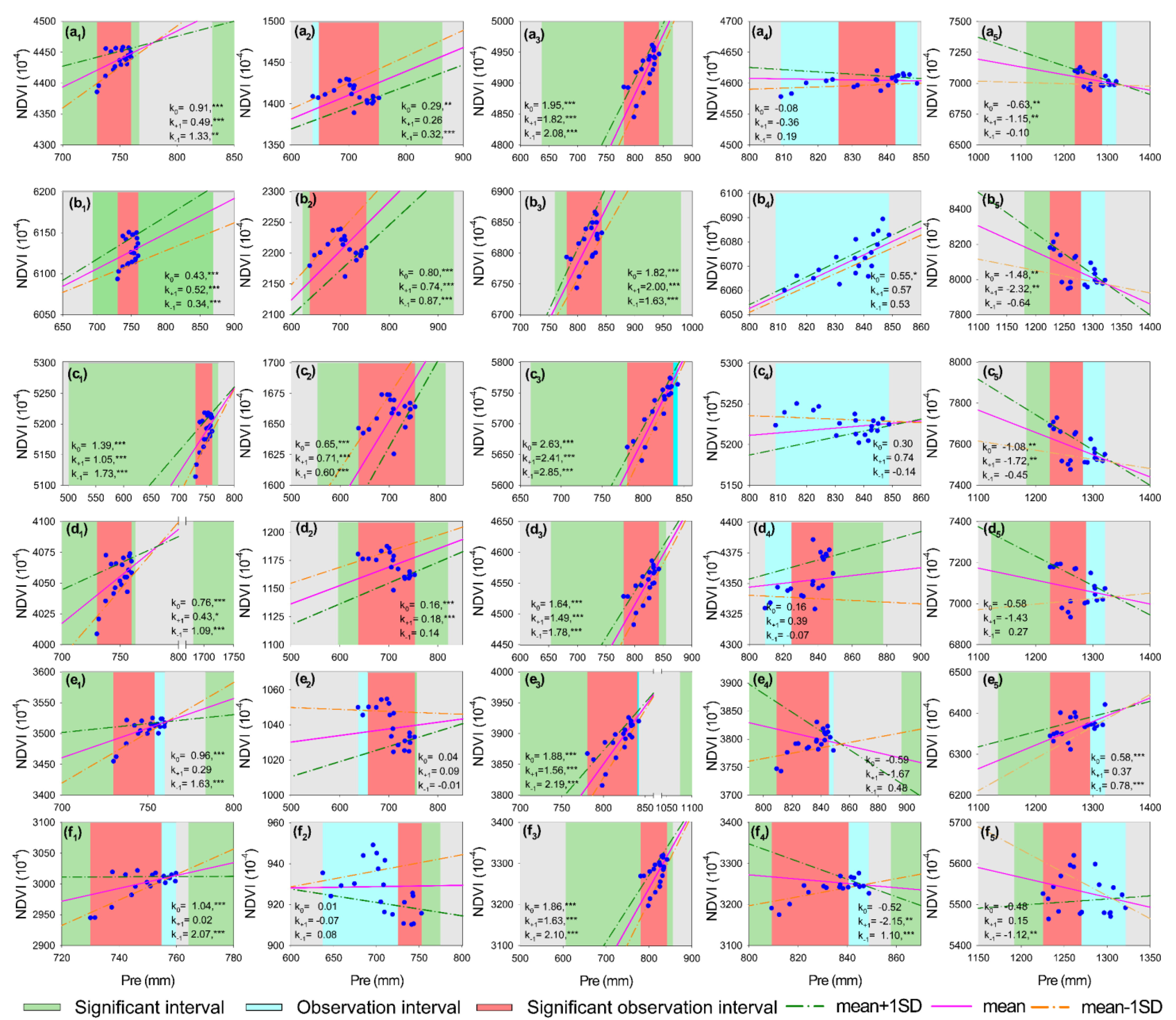
3.2.2. The Regulating Effect of Temperature on the Relationship between Precipitation and NDVI
When the temperature was regulated, precipitation (except NSC area and T+ *–P+ area) could successfully explain the variation trend of NDVI. With increasing precipitation, NDVI progressively declined in the NSC area but increased in SW and other CAs (Figure 3). At the same time, the temperature significantly moderated the regression value of precipitation and NDVI (YNDVI–P), which likewise changed with the increase in precipitation. For example, in the period of P75–P25 in the T+ *–P+ * area, when the precipitation was less than 815.53 mm, 821.35 mm, and 756.89 mm, the temperature had a significant negative moderating effect on YNDVI–P while, with increasing precipitation, the moderating role diminished. Meanwhile, in the Mean, P100, and P5 periods in the T+ *–P+ * area, when the precipitation was more significant than 647.51 mm, 622.59 mm, and 725.17 mm, respectively, the temperature had a significant negative moderating effect on YNDVI–P while, with an increase in precipitation, the temperature regulation effect increased.
According to the J–N method, the temperature moderating effect at P100 and P75 in the T+ *–P+ area was not significant; however, there were significant temperature moderating effects in other cases. In the Mean and P100–P5 periods in the SW region, when the precipitation was in the range of [730.00 mm, 759.88 mm], [730.00 mm, 759.88 mm], [730.00 mm, 759.88 mm], [730.00 mm, 753.95 mm], and [730.00 mm, 754.85 mm] (observed precipitation, [730.00 mm, 759.88 mm]), respectively, the temperature had a significant positive regulation effect on kNDVI–P (Appendix A, Figure A1b). Furthermore, the direction and scope of the significant moderating effect of temperature varied at different vegetation growth stages in the CAs. In general, the significant regulatory impact of temperature was negative in the NSC area and positive in the SW and other CAs.
4. Discussion
4.1. Simple Slope Analysis
Numerous studies have demonstrated that vegetation growth is typically influenced by multiple climate factors, being closely related to hydrothermal conditions (particularly temperature and precipitation) [11,37,60,72], which present complex non-linear interactions under diverse spatial patterns and time scales [30,31]. The multiple linear regression equations established by considering the interaction could effectively establish the regression relationship between NDVI, temperature, and precipitation (p < 0.01), except for the T+ *–P+ * (at P5), NSC (at P5), and T+ *–P+ (at P75) areas. The mean value of the overall coefficients of determination (R2) in the regression equation was as follows (Table 3): SW (0.94 ± 0.02) > T+ *–P– area (0.92 ± 0.02) > T+ *–P+ * area (0.68 ± 0.11) > T+ *–P+ area (0.67 ± 0.16) > NSC area (0.61 ± 0.11), demonstrating that the vegetation growth in the SW and the CAs may be well-explained by temperature and precipitation variables and their interaction, which was essentially consistent with the results of Han et al. [33] in the Inner Mongolia Plateau, where precipitation, temperature, and their interaction explained 88.35% of the change in vegetation primary productivity.
In the T+ *–P+ * area (except P5), the temperature had a significant negative main effect (p < 0.01), while there were significant positive main effects in SW and other CAs (p < 0.01). This demonstrated that temperature in SW and CAs (except the T+ *–P+ * area) plays a promoting role in vegetation growth, in agreement with the outcomes of other researchers in high altitude and northern high latitude regions [17,18,19,20,21,22]. With the aggravation of global warming, the length of vegetation growing season has increased, and photosynthesis has strengthened [23,24,25,26]. Meanwhile, in the T+ *–P+ * area, with an increase in temperature, evaporation is accelerated, the water in the soil is reduced, and the water availability is reduced, thus inhibiting vegetation growth [35,39]. As precipitation is the primary water source in the soil, vegetation growth may be affected by soil moisture; with an increase in precipitation, soil moisture tends to increase [7,27,28,73]. In this study, precipitation in the SW, T+ *–P+ *, and T+ *–P– areas predominantly presented a significant positive main effect (p < 0.01); particularly, in the T+ *–P+ * area, less precipitation could depress soil water content, leading to precipitation becoming the major limiting factor in this region [74]. For example, vegetation growth has been positively correlated with precipitation in tropical Africa [27], Eurasia [7], and the Great Plains of the United States [28]. Nonetheless, vegetation growth was inhibited when the precipitation surpassed the threshold of vegetation response to precipitation. In the NSC areas, Mean, P100, and P75 were the periods of concentrated precipitation, with more precipitation, more water vapor, and more cloudy weather, which is not conducive to air circulation and solar radiation absorption, leading to negative vegetation growth [60].
4.2. Johnson–Neyman Analysis
We comprehensively analyzed the significant effects of temperature and precipitation on vegetation growth, and it was determined that the T+ *–P– was mainly affected by the main effect of precipitation. In contrast, the SW and other CAs were affected primarily by temperature (Table 3). The interaction effect of temperature and precipitation on NDVI was positive in the SW, T+ *–P– (at P100), T+ *–P+ (at P100–P50), and T+ *–P+ (at P75–P25) areas, which may have been due to the temperature, precipitation, and their combination having promoting effects on vegetation growth. The simple slope of temperature (precipitation) obtained by combining Figure 2 and Figure 3 increased with increasing precipitation (temperature), suggesting that, at this point in time (e.g., at P100 in the SW), the precipitation concentration distribution and higher temperature jointly promoted the growth of vegetation, similar to the result of the study of Cong [18] on grassland in the central plateau of the region. The effect of temperature on vegetation activity during the growing season was positively regulated by precipitation, and the positive impact of precipitation on vegetation development increased with the increase in temperature. In contrast, the negative interaction of other annual values may have been due to the negative interaction between the non-synchronicity of temperature and precipitation in the months when different characteristic values arise. When precipitation is inadequate, the temperature rises, and evaporation speeds up, thus diminishing soil moisture and consequently reducing the water supply in the upper soil, leading to the browning of foliage [38,39]. On the contrary, in the period of high precipitation, with more water available, the excess water might repress the development of vegetation [74]. Shen et al. [5] have pointed out that the response of vegetation activity in the Qinghai–Xizang Plateau to warming is governed by precipitation, especially in the alpine steppe, where precipitation is low. In comparison, vegetation in areas with more precipitation is more sensitive to temperature. Further, combined with J–N analysis results, we discovered that the temperature in the NSC area (except for the P25 and P50 periods) was within [15.99, 16.03], and precipitation had a significant negative regulation effect on kNDVI–T. In contrast, the temperature in the SW and other CAs was in the ranges of [4.73 °C, 5.13 °C], [−1.91 °C, −1.39 °C], [5.79 °C, 6.38 °C], and [6.31 °C, 6.36 °C], and precipitation played a significant positive moderating role (Appendix A, Figure A1a). In the T+ *–P+ * area, precipitation was in the range of [725.17 mm, 752.82 mm], and the temperature had a significant negative regulation effect on kNDVI–P; meanwhile, in the SW and other CAs, the positive regulation effect was significant in the ranges [730.00 mm, 753.95 mm], [780.74 mm, 836.89 mm], [825.96 mm, 840.55 mm], and [1225.40 mm, 1279.60 mm] (Appendix A, Figure A1b). Ultimately, by incorporating our results, we can conclude that the reaction of vegetation activity to a single climatic factor A (e.g., temperature) was moderated by another climatic factor B (e.g., precipitation) and that the moderating effect will be adjusted as climatic factor A changes [18,38].
Furthermore, a growing body of research has recognized that vegetation can further regulate local and even global climate change by affecting the carbon cycle’s surface energy balance and biogeochemical properties, altering the exchange of energy and matter between the surface and the atmosphere [6,48,49,75,76]. The main processes involved are evapotranspiration, which controls the climate effect during the day, and albedo feedback, which affects the climate at night and is non-linear. When the albedo is low, the local surface temperature is reduced by evapotranspiration or thermal convection; otherwise, the local surface temperature will increase [5,77,78,79], affecting local precipitation and its distribution pattern, soil moisture and runoff [80]. Zeng et al. have pointed out that, from 1982 to 2011, with the growth of global vegetation, the earth’s land surface temperature increase rate decreased by 0.09 ± 0.02 °C, accounting for 12% of the global land surface warming rate, and the decreasing temperature rate was mainly in the area where the leaf area index increased [48]. Huang [75] has pointed out that recent land-cover changes in Europe have increased the vegetation coverage in Western and Central Europe, leading to a decrease in 0.12 ± 0.20 °C in the average temperature in summer and autumn. On the other hand, during 2003–2012, forest loss resulted in an average biophysical warming of land equal to about 18% of the global biogeochemical signal from CO2-induced land-use change emissions [49]. These results [76,78,79] indicate that the ecological and environmental protection and restoration measures of “returning grazing land to grassland” and “returning farmland to the forest” implemented by the Chinese government in southwest China can reduce the local climate warming and climate risk by increasing the surface coverage and vegetation carbon storage, increasing the surface transpiration rate and reducing local surface temperature. The fifth report from the IPCC [2] has indicated that an increase in vegetation coverage could reduce the temperature in some areas, and the surface radiative forcing was estimated to decrease by 0.15 ± 0.10 Wm–2 from the perspective of surface albedo. A study of the region by Wang [6] has revealed that vegetation cover plays an essential role in mitigating climate change. The correlation coefficients between annual average temperature and annual precipitation variability and vegetation cover were −0.76 and −0.64, respectively. Meanwhile, ever more studies have recognized that the influence of day and night temperature increase on vegetation in the Qinghai–Tibet Plateau is asymmetrical, which plays an essential role in controlling plant phenology and vegetation dynamics [44,45,46,47]. In addition, the increases in temperature and precipitation have somewhat boosted vegetation growth. As precipitation continues to increase, the soil becomes more susceptible to erosion which, according to the RUSLE loss equation, exceeds the ability of vegetation to maintain water and soil. Increased soil loss would inhibit vegetation growth [81] and affect the biogeochemical characteristics of surface energy balance and the carbon cycle, thus further affecting local climate change.
4.3. Study Limitations
Although CRU TS v. 4.02 data and GIMMS NDVI data were processed by interpolation and filtering to eliminate external interference, due to the complex terrain and other environmental factors in southwest China, there were few meteorological stations available in the study area, especially in Qinghai (only seven stations) and Tibet (only 28 stations), which were mainly concentrated in the eastern peripheral regions of the study area [82]. There are almost no meteorological stations in the western part of the study area. The spatial distribution does not conform to the regular discrete distribution, which is far lower than the minimum allowable station network density recommended by the World Meteorological Organization (40–100 stations per 104·km2) in temperate and tropical humid mountains; therefore, it was impossible to present the continuous spatial distribution of water and heat in the study area comprehensively [83], which could add uncertainty to the outcome. Meanwhile, the GIMMS NDVI data were obtained by an optical sensor and thus were limited by the characteristics of the optical sensor [39,60] and may have been significantly affected by the suspension and scattering of aerosols, external weather conditions (cloud, fog), and atmospheric composition [84]. Although the data set was pre-processed using geometric, radiological, and atmospheric corrections to further eliminate cloud interference by Savitzky–Golay filtering [64], the image confidence was decreased due to the low availability of images from June to August [60]. In addition, the 1:1000 vegetation type map and the China Vegetation Zoning map are currently the most detailed maps of vegetation distribution in southwest China. However, they reflect the vegetation situation in the past, which may increase the uncertainty of the results.
Therefore, in further research, we intend to improve the screening of the core area according to the latest research results, as well as dividing different vegetation types (or zonal vegetation) in the core area to explore the spatiotemporal response of vegetation to climate factors. At the same time, future studies of vegetation response to climate factors should be supplemented and improved due to the need for more validation sample data at a large scale. This may make it easier to understand the interaction of climate factors on vegetation growth in Southwest China in a quantitative manner, allowing for a deeper exploration of the underlying causes.
5. Conclusions
In this study, we used a multiple linear regression model with interaction terms to analyze the impacts of main and interaction effects among climate factors on vegetation growth and quantified the degree of mutual regulatory effects of climate factors on vegetation growth according to the simple slope and Johnson–Neyman methods. Therefore, we used CRU and GIMMS NDVI data to investigate the regulating effects of climate factors on vegetation growth in different vegetation growth periods (P100–P5 and Mean value) in the SW and various CAs. Overall, the multiple linear regression model with interaction terms could effectively establish the relationships between NDVI, temperature, and precipitation (p < 0.01), indicating the existence of an interaction effect related to climate change on vegetation growth in the SW and CAs, as well as revealing that the T+ *–P– areas were predominantly affected by the main effect of precipitation. In contrast, the SW and other CAs were mainly affected by temperature. The results further revealed that the response of vegetation activity to the temperature (precipitation) factor was regulated by the precipitation (temperature) factor. The regulating effect of the precipitation (temperature) factor increased with an increase in the temperature (precipitation) factor, thus demonstrating that the regulating effect of precipitation (temperature) is significant in different regions and directions. To a certain extent, our study provides an essential theoretical basis for effectively revealing the impact of climate change on vegetation growth in the context of global climate change, thus improving the interpretation rate of modeling between climate change and vegetation growth.
Author Contributions
Conceptualization, M.W.; methodology, M.W.; software, M.W.; validation, M.W. and Z.A.; formal analysis, M.W.; investigation, M.W.; resources, M.W.; data curation, M.W.; writing—original draft preparation, M.W. and Z.A.; writing—review and editing, M.W. and Z.A.; visualization, M.W.; supervision, M.W.; project administration, M.W.; funding acquisition, M.W. All authors have read and agreed to the published version of the manuscript.
Funding
This research was funded by Chaozhou Special Fund for Human Resource Development, grant number 2023.
Institutional Review Board Statement
Not applicable.
Informed Consent Statement
Not applicable.
Data Availability Statement
The NDVI datasets used in our work can be freely accessed at https://ecocast.arc.nasa.gov/data/pub/GIMMS/, accessed on 18 November 2018. The climate data (CRU_TS4.02) were obtained from https://crudata.uea.ac.uk/cru/data/hrg/, accessed on 18 December 2018.
Conflicts of Interest
The authors declare no conflict of interest.
Appendix A
Figure A1.
(a) The actual range of the significant moderating effect of precipitation on the relationship between temperature and NDVI (kNDVI–T), and (b) the actual range of the significant moderating effect of temperature on the relationship between precipitation and NDVI (kNDVI–P). Note: “*” and “Ns” indicate the significance levels of p < 0.05 and p > 0.05, respectively. If the significance is Ns, the interval length is not shown in the figure and is only represented by the symbol “growth stages +Ns”; “+”and “−” indicate that the temperature (precipitation) had a positive or negative regulating effect on kNDVI–P (kNDVI–T), respectively.

References
- Bell, R.E.; Seroussi, H. History, mass loss, structure, and dynamic behavior of the Antarctic Ice Sheet. Science 2020, 367, 1321–1325. [Google Scholar] [CrossRef] [PubMed]
- IPCC. Climate Change 2013, The Physical Science Basis, Summary for Policymakers; Cambridge University Press: Cambridge, UK, 2013.
- IPCC. Special Report on Global Warming of 1.5 °C; Cambridge University Press: Cambridge, UK, 2018.
- IPCC. Climate Change 2021, The Physical Science Basis. In Contribution of Working Group, I to the Sixth Assessment Report of the Intergovernmental Panel on Climate Change; Cambridge University Press: Cambridge, UK, 2021. [Google Scholar]
- Shen, M.G.; Piao, S.L.; Jeong, S.J.; Zhang, G.X.; Zhang, Y.J.; Yao, T.D. Evaporative cooling over the Tibetan Plateau induced by vegetation growth. Proc. Natl. Acad. Sci. USA 2015, 112, 9299–9304. [Google Scholar] [CrossRef] [PubMed] [Green Version]
- Wang, M.; Jiang, C.; Sun, O.J. Spatially differentiated changes in regional climate and underlying drivers in southwestern China. J. For. Res. 2022, 33, 755–765. [Google Scholar] [CrossRef]
- Piao, S.L.; Wang, X.; Ciais, P.; Zhu, B.; Wang, T.; Liu, J.I.E. Changes in satellite-derived vegetation growth trend in temperate and boreal Eurasia from 1982 to 2006. Glob. Chang. Biol. 2011, 17, 3228–3239. [Google Scholar] [CrossRef]
- Piao, S.L.; Tan, K.; Nan, H.; Ciais, P.; Fang, J.; Wang, T.; Vuichard, N.; Zhu, B. Impacts of climate and CO2 changes on the vegetation growth and carbon balance of Qinghai-Tibetan grasslands over the past five decades. Glob. Planet. Chang. 2012, 98–99, 73–80. [Google Scholar] [CrossRef]
- Zheng, Z.T.; Zhu, W.Q.; Zhang, Y.J. Seasonally and spatially varied controls of climatic factors on net primary productivity in alpine grasslands on the Tibetan Plateau. Glob. Ecol. Conserv. 2020, 21, e00814. [Google Scholar] [CrossRef]
- Fu, Y.; Zhao, H.; Piao, S.L.; Peaucelle, M.; Peng, S.; Zhou, G.; Ciais, P.; Huang, M.T.; Menzel, A.; Penuelas, J.; et al. Declining global warming effects on the phenology of spring leaf unfolding. Nature 2015, 526, 104–107. [Google Scholar] [CrossRef] [Green Version]
- Wang, M.; An, Z. Regional and Phased Vegetation Responses to Climate Change Are Different in Southwest China. Land 2022, 11, 1179. [Google Scholar] [CrossRef]
- Gong, D.Y.; Ho, C.H. Detection of large-scale climate signals in spring vegetation index (normalized difference vegetation index) over the Northern Hemisphere. J. Geophys. Res. 2003, 108, 4498. [Google Scholar] [CrossRef]
- Zhao, M.; Running, S.W. Drought-induced reduction in global terrestrial net primary production from 2000 through 2009. Science 2010, 329, 940–943. [Google Scholar] [CrossRef]
- de Jong, R.; Schaepman, M.E.; Furrer, R.; de Bruin, S.; Verburg, P.H. Spatial relationship between climatologies and changes in global vegetation activity. Glob. Chang. Biol. 2013, 19, 1953–1964. [Google Scholar] [CrossRef]
- Sloat, L.L.; Gerber, J.S.; Samberg, L.H.; Smith, W.K.; Herrero, M.; Ferreira, L.G.; Godde, C.M.; West, P.C. Increasing importance of precipitation variability on global livestock grazing lands. Nat. Clim. Chang. 2018, 8, 214–218. [Google Scholar] [CrossRef]
- Nemani, R.R.; Keeling, C.D.; Hashimoto, H.; Jolly, W.M.; Piper, S.C.; Tucker, C.J.; Myneni, R.B.; Running, S.W. Climate–driven increases in global terrestrial net primary production from 1982 to 1999. Science 2003, 300, 1560–1563. [Google Scholar] [CrossRef] [PubMed] [Green Version]
- Hansen, J.; Ruedy, R.; Sato, M.; Lo, K. Global surface temperature change. Rev. Geophys. 2010, 48, 1–29. [Google Scholar] [CrossRef] [Green Version]
- Cong, N.; Shen, M.G.; Yang, W.; Yang, Z.; Zhang, F.G.; Piao, S.L. Varying responses of vegetation activity to climate changes on the Tibetan Plateau grassland. Int. J. Biometeorol. 2017, 61, 1433–1444. [Google Scholar] [CrossRef] [PubMed]
- Esau, I.; Miles, V.V.; Davy, R.; Miles, M.W.; Kurchatova, A. Trends in normalized difference vegetation index (NDVI) associ-ated with urban development in northern West Siberia. Atmos. Chem. Phys. 2016, 16, 9563–9577. [Google Scholar] [CrossRef] [Green Version]
- Piao, S.L.; Nan, H.; Huntingford, C.; Zeng, N.; Zeng, Z.; Chen, A. Evidence for a weakening relationship between interannual temperature variability and northern vegetation activity. Nat. Commun. 2014, 5, 5018. [Google Scholar] [CrossRef] [Green Version]
- Wang, X.H.; Piao, S.L.; Ciais, P.; Li, J.S.; Friedlingstein, P.; Koven, C.D.; Chen, A.P. Spring temperature change and its impli-cation in the change of vegetation growth in North America from 1982 to 2006. Proc. Natl. Acad. Sci. USA 2011, 108, 1240–1245. [Google Scholar] [CrossRef] [Green Version]
- Li, L.; Zhang, Y.; Wu, J.; Li, S.; Zhang, B.; Zu, J.; Zhang, H.; Ding, M.; Paudel, B. Increasing sensitivity of alpine grasslands to climate variability along an elevational gradient on the Qinghai-Tibet Plateau. Sci. Total Environ. 2019, 678, 21–29. [Google Scholar] [CrossRef]
- Piao, S.L.; Mohammat, A.; Fang, J.; Cai, Q.; Feng, J. NDVI-based increase in growth of temperate grasslands and its responses to climate changes in China. Glob. Environ. Chang. 2006, 16, 340–348. [Google Scholar] [CrossRef]
- Su, F.; Duan, X.; Chen, D.; Hao, Z.; Cuo, L. Evaluation of the Global Climate Models in the CMIP5 over the Tibetan Plateau. J. Clim. 2013, 26, 3187–3208. [Google Scholar] [CrossRef] [Green Version]
- Lehnert, L.W.; Wesche, K.; Trachte, K.; Reudenbach, C.; Bendix, J. Climate variability rather than overstocking causes recent large scale cover changes of Tibetan pastures. Sci. Rep. 2016, 6, 24367. [Google Scholar] [CrossRef] [Green Version]
- Xu, W.X.; Gu, S.; Zhao, X.Q.; Xiao, J.S.; Tang, Y.H.; Fang, J.Y.; Zhang, J.; Jiang, S. High positive correlation between soil tem-perature and NDVI from 1982 to 2006 in alpine meadow of the Three-River Source Region on the Qinghai-Tibetan Plateau. Int. J. Appl. Earth. Obs. Geoinf. 2011, 13, 528–535. [Google Scholar]
- Camberlin, P.; Martiny, N.; Philippon, N.; Richard, Y. Determinants of the interannual relationships between remote sensed photosynthetic activity and rainfall in tropical Africa. Remote Sens. Environ. 2007, 106, 199–216. [Google Scholar] [CrossRef] [Green Version]
- Wardlow, B.D.; Egbert, S.L. Large-area crop mapping using time-series MODIS 250m NDVI data: An assessment for the U.S. central great plains. Remote Sens. Environ. 2008, 112, 1096–1116. [Google Scholar] [CrossRef]
- Kawabata, A.; Ichii, K.; Yamaguchi, Y. Global monitoring of interannual changes in vegetation activities using NDVI and its relationships to temperature and precipitation. Int. J. Remote Sens. 2001, 22, 1377–1382. [Google Scholar] [CrossRef]
- Dieleman, W.I.; Vicca, S.; Dijkstra, F.A.; Hagedorn, F.; Hovenden, M.J.; Larsen, K.S.; King, J. Simple additive effects are rare: A quantitative review of plant biomass and soil process responses to combined manipulations of CO2 and temperature. Glob. Chang. Biol. 2012, 18, 2681–2693. [Google Scholar] [CrossRef]
- Wu, D.; Zhao, X.; Liang, S.; Zhou, T.; Huang, K.; Tang, B.; Zhao, W. Time-lag effects of global vegetation responses to climate change. Glob. Chang. Biol. 2015, 21, 3520–3531. [Google Scholar] [CrossRef]
- Fuhrer, J. Agroecosystern responses to combinations of elevated CO2, ozone, and global climate change. Agric. Ecosyst. Environ. 2003, 97, 1–20. [Google Scholar] [CrossRef]
- Han, F.; Kang, S.; Buyantuev, A.; Zhang, Q.; Niu, J.; Yu, D.; Ding, Y.; Liu, P.; Ma, W. Effects of climate change on primary production in the Inner Mongolia Plateau, China. Int. J. Remote Sens. 2016, 37, 5551–5564. [Google Scholar] [CrossRef]
- Kong, D.; Miao, C.; Borthwick, A.G.L.; Lei, X.; Li, H. Spatiotemporal variations in vegetation cover on the Loess Plateau, China, between 1982 and 2013: Possible causes and potential impacts. Environ. Sci. Pollut. Res. 2018, 25, 13633–13644. [Google Scholar] [CrossRef] [PubMed]
- Wang, H.; Liu, H.; Cao, G.; Sanders, N.J.; Classen, A.T.; He, J.S. Alpine grassland plants grow earlier and faster but biomass remains unchanged over 35 years of climate change. Ecol. Lett. 2020, 23, 701–710. [Google Scholar] [CrossRef] [PubMed] [Green Version]
- Krakauer, N.Y.; Lakhankar, T.; Anadón, J.D. Mapping and Attributing Normalized Difference Vegetation Index Trends for Nepal. Remote Sens. 2017, 9, 986. [Google Scholar] [CrossRef] [Green Version]
- Chen, Y.; Luo, Y.; Mo, W.; Mo, J.; Huang, Y.; Ding, M. Differences between MODIS NDVI and MODIS EVI in response to climatic factors. J. Nat. Res. 2014, 29, 1802–1812. [Google Scholar]
- Mohammat, A.; Wang, X.H.; Xu, X.T.; Peng, L.Q.; Yang, Y.; Zhang, X.P.; Myneni, R.B.; Piao, S.L. Drought and spring cooling induced recent decrease in vegetation growth in Inner Asia. Agric. For. Meteorol. 2013, 178, 21–30. [Google Scholar] [CrossRef]
- Li, P.; Peng, C.; Wang, M.; Luo, Y.; Li, M.; Zhang, K.; Zhang, D.; Zhu, Q. Dynamics of vegetation autumn phenology and its response to multiple environmental factors from 1982 to 2012 on Qinghai-Tibetan Plateau in China. Sci. Total Environ. 2018, 637–638, 855–864. [Google Scholar] [CrossRef]
- Yang, Y.T.; Guan, H.D.; Shen, M.G.; Liang, W.; Jiang, L. Changes in autumn vegetation dormancy onset date and the climate controls across temperate ecosystems in China from 1982 to 2010. Glob. Chang. Biol. 2015, 21, 652–665. [Google Scholar] [CrossRef]
- Zeppel, M.J.B.; Wilks, J.V.; Lewis, J.D. Impacts of extreme precipitation and seasonal changes in precipitation on plants. Biogeosciences 2014, 11, 3083–3093. [Google Scholar] [CrossRef] [Green Version]
- Shen, M.; Piao, S.; Cong, N.; Zhang, G.; Jassens, I.A. Precipitation impacts on vegetation spring phenology on the Tibetan Plateau. Glob. Chang. Biol. 2015, 21, 3647–3656. [Google Scholar] [CrossRef] [Green Version]
- Shi, C.; Shen, M.; Wu, X.; Cheng, X.; Li, X.; Fan, T.; Li, Z.; Zhang, Y.; Fan, Z.; Shi, F.; et al. Growth response of alpine treeline forests to a warmer and drier climate on the southeastern Tibetan Plateau. Agric. For. Meteorol. 2019, 264, 73–79. [Google Scholar] [CrossRef]
- Du, Q.; Yi, G.; Zhou, X.; Zhang, T.; Li, J.; Xie, H.; Hu, J. Analysis of asymmetry in diurnal warming and its impact on vegetation phenology in the Qinghai-Tibetan Plateau using MODIS remote sensing data. J. Appl. Remote Sens. 2021, 15, 028502. [Google Scholar] [CrossRef]
- Shen, M.; Wang, S.; Jiang, N.; Sun, J.; Cao, R.; Ling, X.; Fang, B.; Zhang, L.; Zhang, L.; Xu, X.; et al. Plant phenology changes and drivers on the Qinghai–Tibetan Plateau. Nat. Rev. Earth. Environ. 2022, 3, 633–651. [Google Scholar] [CrossRef]
- Shen, X.; Liu, Y.; Zhang, J.; Wang, Y.; Ma, R.; Liu, B.; Lu, X.; Jiang, M. Asymmetric impacts of diurnal warming on vegetation carbon sequestration of marshes in the Qinghai Tibet Plateau. Glob. Biogeochem. Cycles 2022, 36, e2022GB007396. [Google Scholar] [CrossRef]
- Yang, Z.; Shen, M.; Jia, S.; Guo, L.; Yang, W.; Wang, C.; Chen, X.; Chen, J. Asymmetric Responses of the End of Growing Season to Daily Maximum and Minimum Temperatures on the Tibetan Plateau. J. Geophys. Res. Atmos. 2017, 122, 13278–13287. [Google Scholar] [CrossRef]
- Zeng, Z.Z.; Piao, S.L.; Li, L.Z.X.; Zhou, L.M.; Ciais, P.; Wang, T.; Li, Y.; Lian, X.; Wood, E.F.; Friedlingstein, P.; et al. Climate mitigation from vegetation biophysical feedbacks during the past three decades. Nat. Clim. Chang. 2017, 7, 432–436. [Google Scholar] [CrossRef]
- Alkama, R.; Cescatti, A. Climate change: Biophysical climate impacts of recent changes in global forest cover. Science 2016, 351, 600–604. [Google Scholar] [CrossRef] [Green Version]
- Li, X.C. Historical Geography: Geopolitics, Regional Economy and Culture; Peking University Press: Beijing, China, 2004; pp. 79–93. (In Chinese) [Google Scholar]
- Zhao, W.J. Extreme weather and climate events in China under changing climate. Natl. Sci. Rev. 2020, 7, 938–943. [Google Scholar] [CrossRef] [Green Version]
- You, Q.; Chen, D.; Wu, F.; Pepin, N.; Cai, Z.; Ahrens, B.; Jiang, Z.; Wu, Z.; Kang, S.; Amir, A.K. Elevation dependent warming over the Tibetan Plateau: Patterns, mechanisms and perspectives. Earth-Sci. Rev. 2020, 210, 103349. [Google Scholar] [CrossRef]
- China Meteorological Administration. Blue Book on Climate Change in China 2020; Science Press: Beijing, China, 2020.
- Ganjurjav, H.; Gornish, E.S.; Hu, G.Z.; Schwartz, M.W.; Wan, Y.; Li, Y.; Gao, Q. Warming and precipitation addition interact to affect plant spring phenology in alpine meadows on the central Qinghai-Tibetan Plateau. Agric. For. Meteorol. 2020, 287, 107943. [Google Scholar] [CrossRef]
- Wang, C.; Guo, H.; Zhang, L.; Liu, S.; Qiu, Y.; Sun, Z. Assessing phenological change and climatic control of alpine grasslands in the Tibetan Plateau with MODIS time series. Int. J. Biometeorol. 2015, 59, 11–23. [Google Scholar] [CrossRef]
- Huang, K.; Zhang, Y.; Zhu, J.; Liu, Y.; Zu, J.; Zhang, J. The Influences of Climate Change and Human Activities on Vegetation Dynamics in the Qinghai-Tibet Plateau. Remote Sens. 2016, 8, 876. [Google Scholar] [CrossRef] [Green Version]
- Yuan, J.J.; Guo, J.Y.; Niu, Y.P.; Zhu, C.C.; Li, Z. Mean Sea Surface Model over the Sea of Japan Determined from Multi-Satellite Altimeter Data and Tide Gauge Records. Remote Sens. 2020, 12, 4168. [Google Scholar] [CrossRef]
- Rutherford, A. Applied multiple regression/correlation analysis for the behavioral sciences. Br. J. Math. Stat. Psychol. 2003, 56, 185–186. [Google Scholar]
- Johnson, P.O.; Neyman, J. Tests of certain linear hypotheses and their application to some educational problems. Stat. Res. Mem. 1936, 1, 57–93. [Google Scholar]
- Wang, M.; An, Z.; Wang, S. The Time Lag Effect Improves Prediction of the Effects of Climate Change on Vegetation Growth in Southwest China. Remote Sens. 2022, 14, 5580. [Google Scholar] [CrossRef]
- Harris, I.; Osborn, T.; Jones, P.; Lister, D. Version 4 of the CRU TS monthly high-resolution gridded multivariate climate da-taset. Sci. Data 2020, 7, 1–18. [Google Scholar] [CrossRef] [Green Version]
- Buermann, W.G.; Forkel, M.; O’Sullivan, M.; Sitch, S.; Friedlingstein, P.; Haverd, V. Widespread seasonal compensation effects of spring warming on northern plant productivity. Nature 2018, 562, 110–115. [Google Scholar] [CrossRef] [Green Version]
- Grosso, S.D.; Parton, W.J.; Derner, J.; Chen, M.; Compton, J.T. Simple models to predict grassland ecosystem C exchange and actual evapotranspiration using NDVI and environmental variables. Agric. For. Meteorol. 2018, 249, 1–10. [Google Scholar] [CrossRef]
- Yin, L.; Wang, X.; Feng, X.; Fu, B.; Chen, Y. A Comparison of SSEBop-Model-Based Evapotranspiration with Eight Evapo-transpiration Products in the Yellow River Basin, China. Remote Sens. 2020, 12, 2528. [Google Scholar] [CrossRef]
- Huang, M.; Piao, S.L.; Janssens, I.A.; Zhu, Z.; Wang, T.; Wu, D.; Ciais, P.; Myneni, R.B.; Peaucelle, M.; Peng, S.S.; et al. Velocity of change in vegetation productivity over northern high latitudes. Nat. Ecol. Evol. 2017, 1, 1649–1654. [Google Scholar] [CrossRef] [Green Version]
- Gong, P.; Li, X.; Wang, J.; Bai, Y.; Zhou, Y. Annual maps of global artificial impervious area (GAIA) between 1985 and 2018. Remote Sens. Environ. 2020, 236, 111510. [Google Scholar] [CrossRef]
- Knott, G.D. Interpolating Cubic Splines; Springer Science & Business Media: Berlin, Germany, 2012; pp. 1–244. [Google Scholar]
- Preacher, K.J.; Hayes, A.F. SPSS and SAS procedures for estimating indirect effects in simple mediation models. Behav. Res. Meth. Ins. C 2004, 36, 717–731. [Google Scholar] [CrossRef] [PubMed] [Green Version]
- Hayes, A.F. An Introduction to Mediation, Moderation, and Conditional Process Analysis: A Regression-Based Approach; Guilford Press: New York, NY, USA, 2013. [Google Scholar]
- Spiller, S.A.; Fitzsimons, G.J.; Lynch, J.G.; McClelland, G.H. Spotlights, floodlights, and the magic number zero: Simple effects tests in moderated regression. J. Mark. Res. 2013, 50, 277–288. [Google Scholar] [CrossRef]
- Johnson, T.R. Violation of the Homogeneity of Regression Slopes Assumption in ANCOVA for Two-Group Pre-Post Designs: Tutorial on A Modified Johnson–Neyman Procedure. Quant. Methods Psychol. 2016, 12, 253–263. [Google Scholar] [CrossRef]
- Huang, X.; Zhang, T.B.; Yi, G.H.; He, D.; Zhou, X.B.; Li, J.J.; Bie, X.J.; Miao, J.Q. Dynamic changes of NDVI in the growing season of the Tibetan Plateau during the past 17 years and its response to climate change. Int. J. Environ. Res. Public Health 2019, 16, 3452. [Google Scholar] [CrossRef] [PubMed] [Green Version]
- You, G.; Arain, M.A.; Wang, S.; Zhang, X.H.; Gu, Y.Y.; Gao, J.X. The spatial-temporal distributions of controlling factors on vegetation growth in Tibet Autonomous Region, Southwestern China. Environ. Res. Commun. 2019, 1, 091003. [Google Scholar] [CrossRef]
- Guan, Q.; Yang, L.; Pan, N.; Lin, J.; Xu, C.; Wang, F.; Liu, Z. Greening and Browning of the Hexi Corridor in Northwest China: Spatial Patterns and Responses to Climatic Variability and Anthropogenic Drivers. Remote Sens. 2018, 10, 1270. [Google Scholar] [CrossRef] [Green Version]
- Huang, B.; Hu, X.P.; Fuglstad, G.A.; Zhou, X.; Zhao, W.W.; Cherubini, F. Predominant regional biophysical cooling from recent land cover changes in Europe. Nat. Commun. 2020, 11, 1066. [Google Scholar] [CrossRef] [Green Version]
- Peng, S.S.; Piao, S.L.; Zeng, Z.Z.; Ciais, P.; Zhou, L.M.; Li, L.Z.X.; Myneni, R.B.; Yin, Y.; Zeng, H. Afforestation in China cools local land surface temperature. Proc. Natl. Acad. Sci. USA 2014, 111, 2915–2919. [Google Scholar] [CrossRef] [Green Version]
- Rotenberg, E.; Yakir, D. Contribution of semi-arid forests to the climate system. Science 2010, 327, 451–454. [Google Scholar] [CrossRef]
- Li, L.; Zha, Y.; Zhang, J.H.; Li, Y.M.; Lyu, H. Effect of terrestrial vegetation growth on climate change in China. J. Environ. Manag. 2020, 262, 110321. [Google Scholar] [CrossRef]
- Bright, R.M.; Davin, E.; O’Halloran, T.; Pongratz, J.; Zhao, K.G.; Cescatti, A. Local temperature response to land cover and management change driven by non-radiativeprocesses. Nat. Clim. Chang. 2017, 7, 296–302. [Google Scholar] [CrossRef]
- Zeng, H.L.; Ji, J.J.; Wu, G.X. Numerical experiment of the influence of global vegetation distribution on climate. Chin. J. Atmos. Sci. 2010, 34, 1–11, (In Chinese with English abstract). [Google Scholar]
- Xiong, M.Q.; Sun, R.H.; Chen, L.D. A global comparison of soil erosion associated with land use and climate type. Geoderma 2019, 343, 31–39. [Google Scholar] [CrossRef]
- Wang, M.; Wang, H.S.; Jiang, C.; Sun, J.X. Spatial soil erosion patterns and quantitative attribution analysis in Southwestern China based on RUSLE and Geo-Detector model. J. Basic Sci. Eng. 2021, 29, 1386–1402, (In Chinese with English abstract). [Google Scholar]
- Wang, X.P.; Tang, Z.Y.; Fang, J.Y. Climatic control on forests and tree species distribution in the forest region of Northeast China. J. Integr. Plant Biol. 2006, 48, 778–789. [Google Scholar] [CrossRef]
- Nagol, J.R.; Vermote, E.F.; Prince, S.D. Effects of atmospheric variation on AVHRR NDVI data. Remote Sens. Environ. 2009, 113, 392–397. [Google Scholar] [CrossRef]
Figure 1.
Outline of: (a) Geography; (b) vegetation divisions; and (c) vegetation types in the SW region.
Figure 1.
Outline of: (a) Geography; (b) vegetation divisions; and (c) vegetation types in the SW region.

Figure 2.
The regulating effect of precipitation on the relationship between temperature and NDVI. Mean and mean ± 1SD denote the regression equations established by temperature and NDVI when the precipitation was set as the mean and mean ± 1SD, respectively, and the corresponding simple slopes are k0 and k±1. Significant intervals indicate the temperatures at which the precipitation presented a significant moderating effect, according to the J–N analysis range. The observation interval represents the actual observation interval of temperature. A significant observation interval indicates the actual temperature range for which the precipitation presented a significant regulation effect. Note: (a–f) refer to Mean, P100, P75, P50, P25, and P5, respectively; (1–5) refer to SW, T+ *–P+ *, T+ *–P–, T+ *–P+, and NSC, respectively. * p < 0.05, ** p < 0.01, *** p < 0.001.

Figure 3.
The regulatory effect of temperature on the relationship between precipitation and NDVI. Mean and mean ± 1SD denote the regression equations established between precipitation and NDVI when the temperature was set to the mean and mean ± 1SD, respectively, and the corresponding simple slopes are k0 and k±1. Significant interval indicates the precipitation at which the temperature presented a significant moderating effect, according to the J–N analysis range. The observation interval represents the actual observation interval of precipitation. Significant observation interval indicates the actual precipitation range for which the temperature presented a significant regulating effect. Note: (a–f) refer to Mean, P100, P75, P50, P25, and P5, respectively, while (1–5) refers to the SW, T+ *–P+ *, T+ *–P–, T+ *–P+, and NSC areas, respectively. * p < 0.05, ** p < 0.01, *** p < 0.001.


Table 1.
The source of main data and related description.
| Name | Sources | Resolution | Web Site | Access Date | Format |
|---|---|---|---|---|---|
| GIMMS NDVI3g | GIMMS | 8 × 8 km | https://ecocast.arc.nasa.gov/data/pub/GIMMS/ | 18 November 2018 | .nc4 |
| CRU_TS4.02 | Climate Research Unit | 0.5° × 0.5° | https://crudata.uea.ac.uk/cru/data/hrg/ | 28 June 2019 | .nc |
| Global Artificial Impervious Area | Tsinghua university data | 30 × 30 m | http://data.ess.tsinghua.edu.cn | 31 December 2019 | .tif |
| China’s vegetation zoning data | Resource and Environment Science and Data Center | — | http://www.resdc.cn/data.aspx?DATAID=133 | 1 December 2017 | .shp |
Table 2.
Test results when the simple slope was significant. is the moderator variable; and refer to the greatest and least values of , respectively; and and are the solutions of the binary first-order Equation (17) for .
Table 2.
Test results when the simple slope was significant. is the moderator variable; and refer to the greatest and least values of , respectively; and and are the solutions of the binary first-order Equation (17) for .
| Types | Criterion | Range of Possible Values of the Moderator Variable |
|---|---|---|
| Sort 1 | ||
| Sort 2 | ||
| Sort 3 | ||
| Sort 4 |
Table 3.
Multiple linear regression results of vegetation NDVI with temperature and precipitation using a 15-year sliding window. T+ *–P+ *, significant increases in temperature and precipitation; T+ *–P−, a significant increase in temperature related to a decrease in precipitation; T+ *–P+, a significant increase in temperature related to an increase in precipitation; NSC, no significant change. “+/−” in the upper right corner denotes an increase/decrease in temperature or precipitation; Temperature × Precipitation represents the interaction term between temperature and precipitation; R2 represents the entire model’s overall coefficient of determination. “*” and “**” to the right of the numbers represent the significance of the regression coefficient and overall model at the 0.05 and 0.01 levels, respectively.
| Annual Characteristic Value | Characteristic Index Value | SW | T+ *–P+ * | T+ *–P– | T+ *–P+ | NSC |
|---|---|---|---|---|---|---|
| Temperature | 0.64 ** | −1.43 ** | 0.68 ** | 0.73 * | 0.58 ** | |
| Mean | Precipitation | 0.41 ** | 0.91 * | 1.05 ** | −0.09 | −0.34 * |
| Temperature × Precipitation | −0.19 ** | −0.09 | −0.07 | −0.30 | −0.29 | |
| R2 | 0.97 ** | 0.67 ** | 0.94 ** | 0.59 ** | 0.69 ** | |
| Temperature | 0.92 ** | −1.63 ** | 0.87 ** | 0.23 | 0.45 * | |
| P100 | Precipitation | 0.23 ** | 1.36 ** | 0.95 ** | 0.65 | −0.47 * |
| Temperature × Precipitation | 0.05 | −0.11 | 0.10 | 0.03 | −0.27 | |
| R2 | 0.96 ** | 0.75 ** | 0.91 ** | 0.68 ** | 0.64 ** | |
| Temperature | 0.67 ** | −1.66 ** | 0.36 ** | -0.67 | 0.50 ** | |
| P75 | Precipitation | 0.45 ** | 1.75 ** | 1.10 ** | 0.26 | −0.42* |
| Temperature × Precipitation | −0.11 | 0.14 | −0.09 | 0.38 | −0.25 | |
| R2 | 0.95 ** | 0.71 ** | 0.94 ** | 0.37 | 0.64 ** | |
| Temperature | 0.63 ** | −1.29 ** | 0.68 ** | 0.84 ** | 0.62 ** | |
| P50 | Precipitation | 0.40 ** | 0.50 | 1.03 ** | 0.11 | −0.21 |
| Temperature × Precipitation | −0.17 * | 0.07 | −0.09 | 0.16 | −0.30 | |
| R2 | 0.92 ** | 0.79 ** | 0.91 ** | 0.80 ** | 0.63 ** | |
| Temperature | 0.42 ** | −0.91 * | 0.53 ** | 0.93 ** | 0.66 ** | |
| P25 | Precipitation | 0.46 ** | 0.12 | 1.09 ** | −0.31 | 0.67 ** |
| Temperature × Precipitation | −0.32 ** | 0.15 | −0.18 * | −0.57 * | −0.24 | |
| R2 | 0.90 ** | 0.68 ** | 0.94 ** | 0.81 ** | 0.70 ** | |
| Temperature | 0.42 ** | −0.68 | 0.80 ** | 0.74 ** | −0.42 | |
| P5 | Precipitation | 0.41 ** | 0.02 | 0.93 ** | −0.24 | −0.30 |
| Temperature × Precipitation | −0.40 ** | −0.20 | −0.12 | −0.74 ** | 0.40 | |
| R2 | 0.97 ** | 0.45 * | 0.89 ** | 0.80 ** | 0.36 |
Disclaimer/Publisher’s Note: The statements, opinions and data contained in all publications are solely those of the individual author(s) and contributor(s) and not of MDPI and/or the editor(s). MDPI and/or the editor(s) disclaim responsibility for any injury to people or property resulting from any ideas, methods, instructions or products referred to in the content. |
© 2023 by the authors. Licensee MDPI, Basel, Switzerland. This article is an open access article distributed under the terms and conditions of the Creative Commons Attribution (CC BY) license (https://creativecommons.org/licenses/by/4.0/).
Share and Cite
MDPI and ACS Style
Wang, M.; An, Z. Quantifying the Interaction Effects of Climatic Factors on Vegetation Growth in Southwest China. Remote Sens. 2023, 15, 774. https://0-doi-org.brum.beds.ac.uk/10.3390/rs15030774
AMA Style
Wang M, An Z. Quantifying the Interaction Effects of Climatic Factors on Vegetation Growth in Southwest China. Remote Sensing. 2023; 15(3):774. https://0-doi-org.brum.beds.ac.uk/10.3390/rs15030774
Chicago/Turabian StyleWang, Meng, and Zhengfeng An. 2023. "Quantifying the Interaction Effects of Climatic Factors on Vegetation Growth in Southwest China" Remote Sensing 15, no. 3: 774. https://0-doi-org.brum.beds.ac.uk/10.3390/rs15030774
Note that from the first issue of 2016, this journal uses article numbers instead of page numbers. See further details here.