1. Introduction
As modern space satellite technology has developed by leaps and bounds in recent decades, the application of remote sensing images has multiplied in military and civilian fields, including in environmental monitoring and assessment [
1,
2], resource distribution applications [
3,
4], military reconnaissance and analysis, and other fields. High-quality remote sensing images [
5] are widely employed in ecological indicators’ mapping, urban–rural management, water resource management, hydrologic models, wastewater treatment, water pollution, and urban planning.
In general, the resolution of remote sensing image increases with the expansion of information content in the image, which leads to a high-quality remote sensing image [
6]. However, the spatial resolution and clarity of remote sensing images are inherently low due to the limits of the imaging equipment, image transmission mode, and large satellite detection distance. In view of the high research costs and long development cycle required to improve imaging hardware, it is increasingly vital to apply super-resolution reconstruction algorithms to obtain high-quality remote sensing images.
Image super-resolution aims to reconstruct a high-resolution (HR) image from a relative low-resolution (LR) image, which utilizes the software algorithm to improve the image resolution and avoid the hardware restrictions [
7]. At present, SR is widely employed in the reconstruction of natural images. Remote sensing images contain rich land cover, leading to the distribution of textural details and high-frequency information that differs from those of natural images. Thus, it is difficult to directly apply the existing SR methods for natural images to remote sensing images. Remote sensing images are composed of complex scenes in which objects undergo extensive changes, and there are multiple objects of different sizes intertwined in one scene, resulting in weak correlations, that is, image context features between pixels and surrounding pixels in the images. These are weak, which has an adverse impact on image quality in the super-resolution reconstruction of remote sensing images [
8].
Generally, SR methods enhance the quality of reconstructed images by augmenting the designed network depth. Reference-based image super-resolution (RefSR) introduces an additional reference image, transfers the image details to a low-resolution image, and accomplishes image reconstruction with supplementary information, which is separate from the main network [
9]. Meanwhile, the inherent longitude and latitude information of remote sensing images also makes it more expedient to obtain a reference image with the same coordinates as the LR image.
To address the aforementioned problem, we proposed a remote sensing image super-resolution method based on the reference image. By extracting the reference image texture information, along with the feature matching and exchange between the LR and Ref images, more multi-level feature information is provided for remote sensing image super-resolution. The major contributions of this paper are as follows:
- (1)
We proposed a novel super-resolution method FCSR to enrich the context features of remote sensing images from multiple perspectives. The network improves the lack of context features for remote sensing images in three aspects and achieves significant results for the SR task for remote sensing images;
- (2)
In FCSR, we designed a novel feature compression branch. The branch was employed for the sparse feature processing of LR and Ref images to remove redundant image information. The remaining features were extracted, matched, and exchanged via the texture-swapping branch to supplement the context features that the remote sensing images lack;
- (3)
We proposed and exploited the use of FEE to develop a texture-swapping branch. FEE is a portion of the encoder in the multi-level self-encoder. The encoding module can extract ample multi-level features in the – image pairs, improve the extent of matching between the LR remote sensing image and the corresponding Ref image, and effectively increase the resemble features contained in the image. In addition, FEE lays a solid foundation for the subsequent feature exchange in the texture-swapping branch.
The remaining sections of this paper are organized as follows:
Section 2 introduces the related work.
Section 3 details the proposed network.
Section 4 demonstrates the outcomes of the ablation experiments and compares these with several SR algorithms.
Section 5 illustrates the ablation study, and
Section 6 summarizes the entire study and outlines potential future study directions.
2. Related Work
2.1. Image Super-Resolution
In recent years, a great deal of researches were conducted on super-resolution reconstruction. The existing SR algorithms [
10] can generally be divided into three categories: super-resolution based on interpolation, super-resolution based on reconstruction, and super-resolution based on learning. The early super-resolution methods utilizing interpolation include bicubic linear interpolation [
11], but their ability to process image edges and details is poor, and it is easy to produce sawtooth oscillation. A super-resolution method based on reconstruction makes the most of the prior image knowledge to obtain a relatively good reconstruction effect, such as the convex set projection method [
12], but it is difficult to obtain sufficiently accurate prior information.The learning-based method does not need to use the prior image knowledge. This establishes the relationship between the LR image and its corresponding HR image through training and learning. The learning-based method can better extract the high-frequency image information than the method, based on neighborhood embedding [
13], the method based on sparse representation [
14], and the method based on deep learning [
7]. However, the first two methods mostly use the shallow image features for SR reconstruction, and focusing only on these features greatly limits the reconstruction effect.
With the rapid progression and development of the computing power of big data and the graphics processing unit (GPU), the convolutional neural network (CNN) has become the leading method in the field of image processing [
15]. The CNN-based method shows strong competency in automatically premising deep features from data, which provides a very practical method for improving image resolution. The basic principle of the SR reconstruction method based on CNN is to use a dataset including HR images and comparative LR images to train a model. The model takes an LR image as input and outputs SR images.The SRCNN [
7] algorithm proposed by Dong et al. firstly applied CNN to SR reconstruction, which learned the mapping relationship between LR and HR by constructing three convolution layers, but the network receptive field was relatively small, and the extracted features were very local, so the global distribution of the image cannot be recovered. The VDSR [
16] algorithm proposed by Kim et al. employed the deep ResNet [
17] network in image super-resolution reconstruction. Although the network had a certain depth, it did not take full advantage of the feature information contained in the LR image.
The generative adversarial network (GAN) [
18] is also utilized for the super-resolution reconstruction of images. Ledig et al. proposed an SRGAN [
19] with perceptual loss and a generative adversarial network, which can form more natural textures on a single image SR. Although the blurred and over-smooth image details can be somewhat reduced, the reconstruction results were not very realistic and produced unpleasing artifacts. Wang et al. introduced the residual dense block (RRDB) and proposed an ESRGAN [
20] network based on SRGAN, which engendered more realistic and natural textures and improved visual quality. Ma et al. proposed a super-resolution method SPSR [
21] to preserve the structure, which utilized a gradient map to reveal the sharpening degree of each local area to guide image reconstruction, so as to form well-perceived texture details. Although the generative adversarial network can engender better image details, it is difficult to stably achieve Nash equilibrium, which affects the effectiveness of training and convergence.
2.2. Image Super-Resolution for Remote Sensing Images
SR technology can provide richer spatial details to aerial remote sensing images by improving the resolution of input LR images. However, remote sensing images differ from natural images. The texture features of the image are represented by pixels in different spatial positions and their surrounding surface structures, which change slowly or periodically, reflecting the spatial distribution information of land cover on the image. Moreover, the objects contained in remote sensing image are often coupled with the surrounding environment, and the image scale span is relatively large [
22].
By extracting features from multiple scales, Xu et al. proposed a deep memory connection network DMCN [
23], which established local and global memory connections and combined image details with environmental information. Ma et al. proposed another CNN super-resolution network structure, WTCRR [
24], which included wavelet transform, local residual, and global residual connection. This network combined frequency domain information to solve the super-resolution issues in remote sensing images. The existing super-resolution reconstruction methods for remote sensing images are faced with the following main dilemmas: the distance between the remote sensing satellite camera and the target object is far, the remote sensing image is wide, the scale of the target object in the images greatly changes, and remote sensing images contain more land cover than ordinary, natural images. The existing super-resolution reconstruction methods for natural images are not ideal for direct application to the super-resolution reconstruction of remote sensing images.
2.3. Reference-Based Image Super-Resolution
Reference-based image super-resolution (RefSR) provides additional information from the reference image to shrink the discomfort in image super-resolution, and achieved good results when reconstructing high-frequency details [
25]. In the RefSR task, textural details are transferred to the LR image according to the Ref image, providing more shallow features for image super-resolution reconstruction.
Landmark [
26] globally matched the blocks between LR features and the downsampled Ref features, but there is a problem of mismatch between blocks due to the visual gap and large resolution deviation (8x) between the high-resolution reference image and the LR image. Zheng et al. proposed a method called CrossNet [
27] which employed an optical flow to transfer high-frequency details of a high-resolution Ref image to an LR image. Cross-scale warping and fusion decoder were applied, but the optical flow is limited in its ability to match long-distance correspondences, which may lead to redundant texture information, resulting in serious degradations in performance. Zhang et al. proposed the SRNTT [
28] method, which applied patch-matching between features premised from LR and Ref images, using VGG19 [
29] to exchange similar texture features. Dong et al. proposed a gradient-assisted feature alignment method, RRSGAN [
30], which transferred the textural information in the reference features to the reconstructed super-resolution image.
At present, there are three main challenges in the application of super-resolution Ref images to remote sensing images: (i) there are potential differences in resolution, brightness and contrast, and diversities in the ambiguity between LR and Ref images at the same coordinate position, as determined by the longitude and latitude information of input image, which have a potential effect on the SR procedure; (ii) compared with natural images, the richer ground feature information and larger scale span in remote sensing images make the correlation between adjacent pixels, that is, context features, more deficient, which increases the difficulties in feature matching between LR and Ref images according to the corresponding relationship; (iii) the pretrained model of VGG19, a commonly used feature extraction module, is trained by natural images, and there is a problem of mismatch when extracting features from remote sensing images, which further affects the acquisition of resemble features between LR and Ref images. Focusing on these three obstacles, this paper studies the reference-based super-resolution reconstruction for remote sensing images.
3. Methodology
As mentioned above, the direct application of the SR method based on the Ref image to remote sensing images is confronted with three issues. The first is the resolution gap between LR and Ref images. The second is the diversity in brightness, contrast, and ambiguity, the lack of context features caused by abundant land cover, and the wide-scale span of remote sensing images. The last issue is the incompatibility of remote sensing image features with the VGG19 pretrained with natural images. To conquer these foregoing problems to some extent, we propose a reference-based super-resolution method with a feature compression module (FCSR) for remote sensing images.
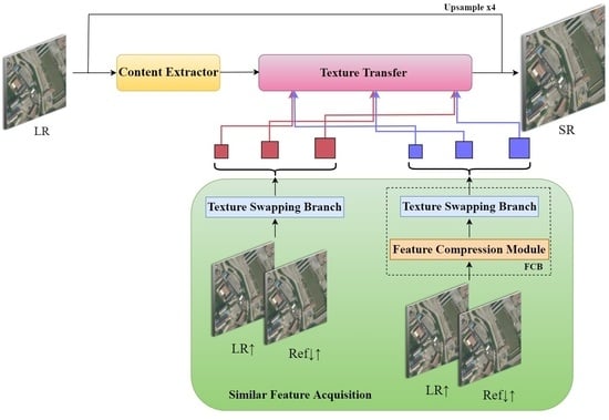
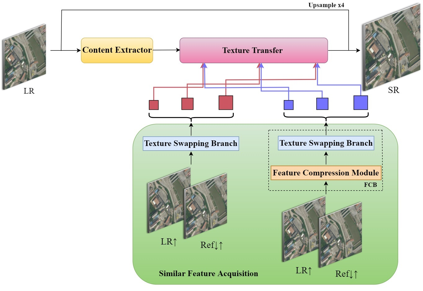
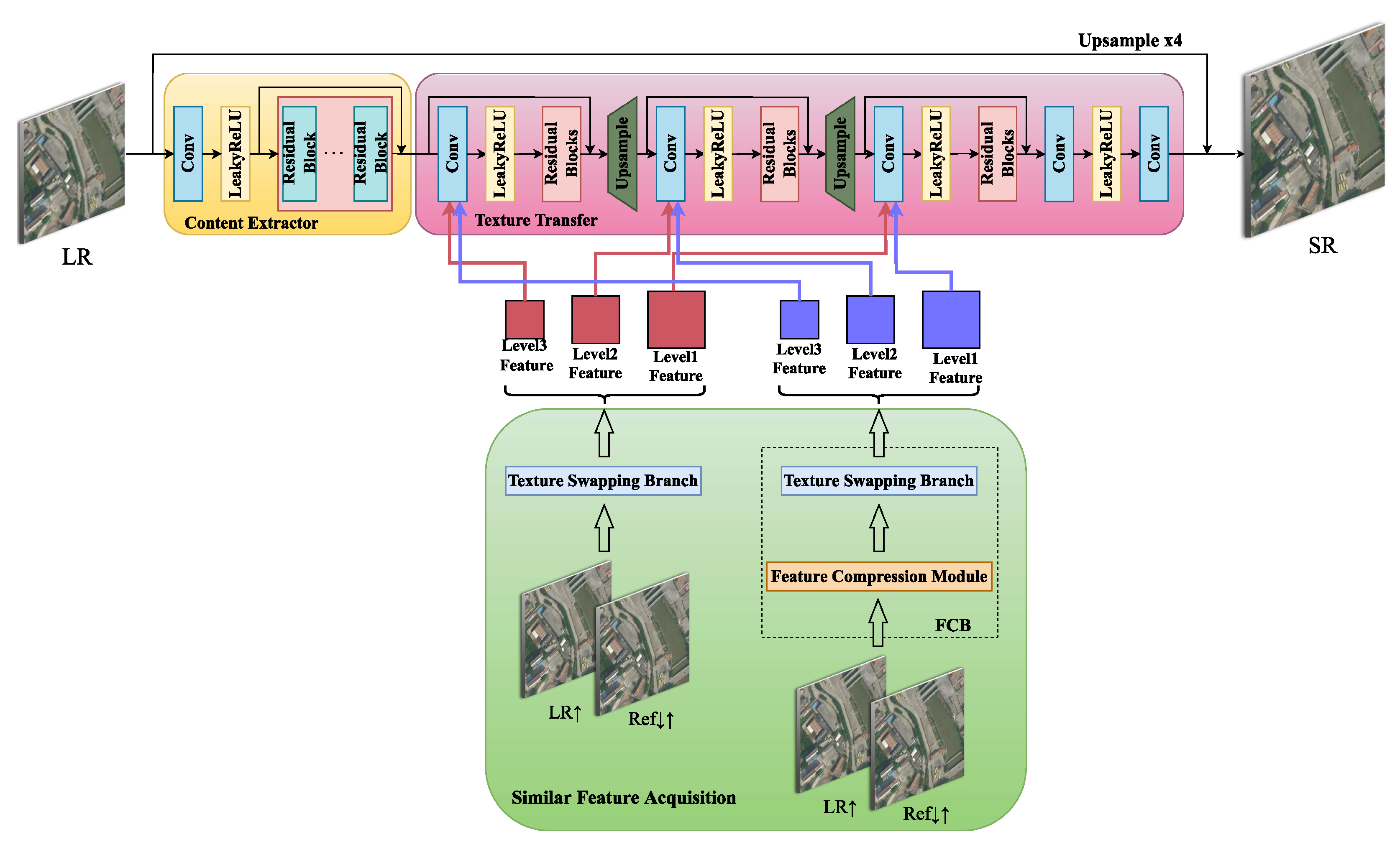
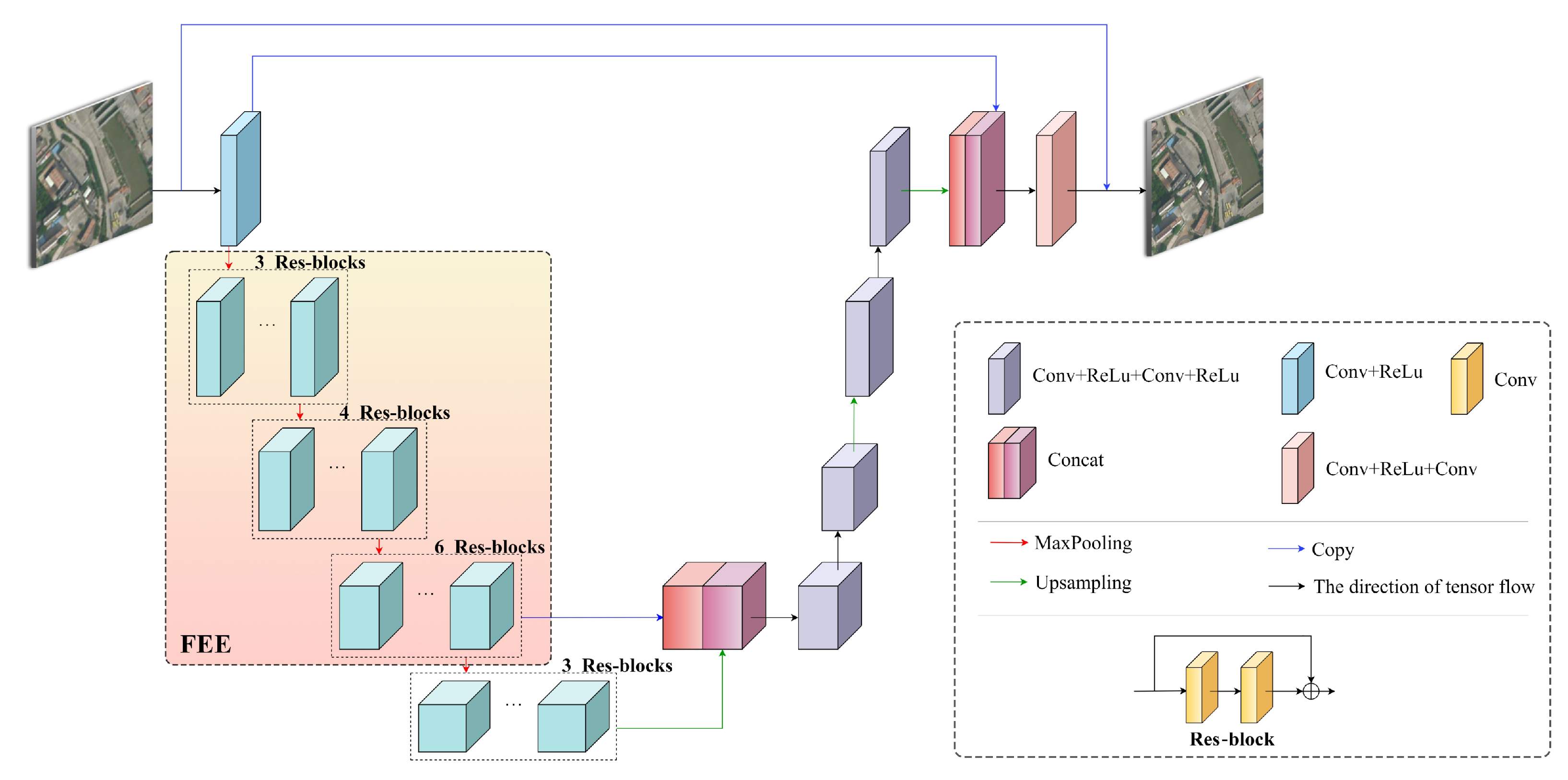
As shown in
Figure 1, the designed network structure is divided into three parts: content extractor, similar feature acquisition, and texture transfer. The content extractor preliminarily extracted the input image information. Similar feature acquisition fulfilled the feature matching between the Ref image and the LR input image. Texture transfer concatenated the reference image information to the LR image to obtain an HR image. Moreover,
represents a low-resolution image, while
stands for a ×4 bicubic-upsampled low-resolution image, and
denotes a high-resolution reference image, which is downsampled and then upsampled.
In terms of similar feature acquisition, we creatively introduce a feature compression branch (FCB) to effectively extract crucial features. Particularly, FCB was designed to utilize a single-value decomposition (SVD) [
31] algorithm to derive sparse features of
and
↑ and match the image feature counterparts. The branch adopted a feature compression module (FCM) to separate features from LR and Ref image textures, furnishing texture transfer with plentiful and useful information from different perspectives. The FCM compressed the features of
–
image pairs and removed the redundant information in the images. This also notes the texture detail counterparts in the image pairs and balances the implicit matching relationship with
–
image pairs, which were not processed by FCM, via the texture swapping branch, in compliance with the resemblance between content and appearance. Furthermore, it embedded similar texture features in the texture transfer section.
To reduce the influence of the resolution gap, brightness, and ambiguity disparity between LR and Ref images, we designed a novel feature extraction encoder (FEE) in FCM to ensure precision in feature extraction using the feature compression branch. FEE is the coding segment of a multi-level self-encoder and can provide rich multi-level features in and image pairs. The multi-level self-encoder is composed of an encoder and a decoder. Remote sensing images in the training set were used to pretrain the multi-level self-encoder. FEE is a portion of the encoder in the multi-level self-encoder, which ensures the extraction of similar features between the LR remote sensing image and the Ref image to a certain extent, to more practically complete the feature matching of image pairs and the subsequent feature exchange. In the two branches of similar feature acquisition, FEE is used to replace VGG19, which is often used in SR procedures and is pretrained using natural images, which is conducive to extracting abundant multi-level features in remote sensing images.
3.1. Feature Compression Branch (FCB)
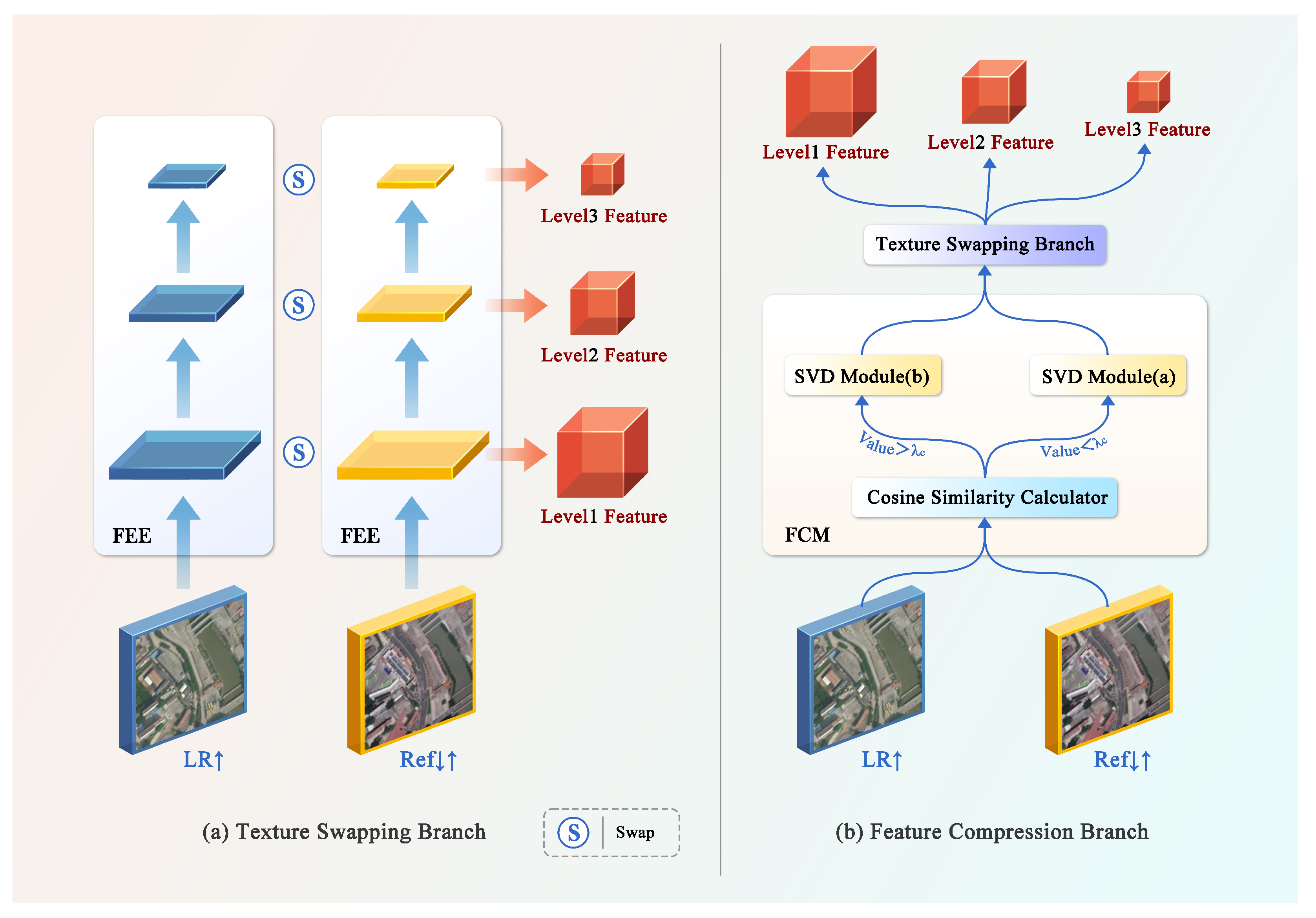
The collected remote sensing images intrinsically possess a low resolution and lack high-frequency information, and the image scale span is large, leading to fewer context features being obtained. Therefore, it is difficult to reconstruct accurate, high-frequency details of real ground cognition in remote sensing images to supply more accurate information. In the course of reconstructing high-quality remote sensing images, it is more rational to precisely offer content that resembles the details of LR remote sensing images than to generate image textures. We proposed a FCB that could provide textural information for texture transfers. The FCB is made up of two sections, as depicted in
Figure 2b. The first segment, FCM, adaptively adjusts the variable parameter size in the SVD module through which the image passes subject to the cosine similarity of the
–
image pairs, providing supplementary information for feature matching of the reconstructed image. The second component is the texture-swapping branch.
Figure 2a indicates that the LR remote sensing image and the Ref image obtain access to three feature levels of different scales after passing through the FEE modules, namely, Level 1 features, Level 2 features, and Level 3 features. These features were swapped in line with the corresponding levels to complete the matching and exchange of image pairs’ feature information; then, the three obtained feature levels are offered three different positions in the texture transfer section.
The SVD employed in the FCM denotes the product of some simple matrices decomposed from a complex matrix, while retaining momentous characteristics. An arbitrary
m ×
n matrix
A can be decomposed into the product of three matrices, which can be expressed as
where
U and
V are column orthonormal matrices, and their column vectors are unit vectors that are orthogonal to each other, satisfying
,
; where,
I is the unit matrix.
is a diagonal matrix, and the values on the main diagonal
are all nonnegative values. The singular value of matrix
A is given by placing these values in descending order, from large to small. In particular,
,
. In the SVD procedure, the substantial characteristics of matrix
A are compressed and decomposed into each matrix. As the scale of singular values rapidly decays and coincides with the compressed representation information of the resolved vector fragments, the sum of the first 10% or even 1% of singular values accounts for more than 99% of the total singular values; that is, the largest
k singular values and the corresponding
U,
V matrix column vectors can approximately represent the matrix
A. For a color image, the R matrix, G matrix, and B matrix, representing three channels, are decomposed into singular values, and
k specified eigenvalues are selected to reconstruct different channel matrices after compression by using
; then, the three single channel matrices processed by SVD are combined to obtain the image compression features.
According to the SVD characteristics, which can compress color images while maintaining dominant information, disposing of sparse features and removing redundant information, we proposed an adaptive FCM that can provide more complementary information about congruous and features for the feature exchange component of the proffered network. First, we calculated the cosine similarity of and , which determines the correlation between the two images. The proportion of a singular value qualified for SVD procedure was adaptively selected to conform with the cosine similarity. Specifically, when the cosine similarity was less than or equal to , the ratio of singular values taken was set to a; when cosine similarity was greater than , the ratio of singular values was set to b to reasonably diminish mismatched feature interference. On the strength of this pre-experiment, we confirm that the values of are 0.88, 0.1, and 0.2. Then, we employed the texture swapping branch to obtain the feature information that is concatenated to the texture transfer section.
3.2. Feature Extraction Encoder
With regard to the reference-based super-resolution task for remote sensing images, the rational matching of comparative slices between LR remote sensing images and Ref images is important. Nevertheless, there are deviations in brightness, chromaticity, contrast, and resolution between the LR and the Ref images. Despite the fact that the content texture has analogical fragments in the two corresponding images, different representations are given in the images due to scale. To moderate the differences in resolution between the two images, a feature extraction encoder was proposed to extract adequately similar features for the LR and Ref images. Pre-upsampling LR images can effectively reduce the diversities in resolution between the two images and emphasize the multi-scale features of images that are indispensable for texture matching.
Given an LR image
and a Ref image
,
denotes an upsampling LR image that has the same resolution as the Ref image.
designates a downsampled then upsampled Ref image. Compared with
–
,
–
emphasizes intrinsic image information. The encoder designed in this paper was utilized to extract multi-level features of
and
. Specifically, FEE was exerted to extract features of three scales. By combining U-Net [
32] with residual theory, we obtained complementary textural information, assuring that the features obtained by the encoder were restored as much as possible when pretraining the multi-level self-encoder, thus greatly curtailing the disparities in resolution between
–
image pairs. Concerning the deviations in luminosity, chromaticity, and saturation, we strengthened the generalization ability of the multi-level self-encoder using the data augmentation of different transformations for the training set images. Meanwhile, FEE more accurately analyze the correlative relationship between
and
, the same FEE was utilized to extract the features of the
and
images after they passed through the FCM.
Considering the weak correlation between adjacent pixels in the remote sensing image, we designed a multi-level self-encoder. The FEE in the encoder module captures more context information from different scales, as revealed in
Figure 3. The multi-level self-encoder was split into an encoder and decoder. The encoder module was exerted to extract the multi-level features of remote sensing images, and the decoder module reconstructed the multi-level features extracted by the encoder module to recover as much of the input remote sensing image information as possible. FEE employed Res-Blocks as a coding module to extract three levels of different scale features from remote sensing images. The structure of the Res-blocks is shown in
Figure 3.
Table 1 displays the network parameter setting details of FEE. The convolution hierarchy can effectively extract image features, while skip connection is introduced to diminish the vanishing gradient problem. This can also prevent over-fitting and improve the precision of the trained model.
Furthermore, in the decoder module, the feature information procured by the encoder module was introduced by skip connection. Meanwhile, the features disposed by the upsampling and convolution modules were concatenated between channels, which relieves the spatial information loss caused by the downsampling procedure and maintains the obliterated information of different layers in the coding section. Remote sensing images in the training set were utilized to pretrain the multi-level self-encoder, the convergence of the model was accelerated, and the generalization ability of the model was strengthened through transfer learning.
Considering the complex surface information of remote sensing images, it is very important to increase the receptive field in the middle of the module to obtain relatively detailed information. Exerting the pooling layer enlarges the receptive field of the corresponding feature layer. When extracting features, we used FEE to extract three levels of remote sensing image features.
3.3. Loss Function
To sustain the spatial structure of LR images, improve the visual quality of SR images, and make the most of the texture information of Ref images, the loss function of network in this paper combines reconstruction loss, perception loss, and adversarial loss. During training, our purpose was to: (i) preserve the spatial structure and semantic information of LR images; (ii) exploit more texture information from Ref images; (iii) synthesize high-quality real SR images. To this end, the total loss calculated using the hyperparameters
and
is described as follows:
Reconstruction loss. To better preserve the spatial structure of LR images and make
closer to
, we adopted the
norm, which is defined as follows:
Perceptual loss. For better visual quality, we adopted the perceptual loss, which is defined as follows:
where
V and
C, respectively, represent the volume and channel number of the feature graph,
represents the Frobenius norm, and
represents the
ith channel of the feature graph extracted from the hidden layer of the feature extraction model.
Adversarial loss. In order to further generate images with natural details and good visual effects, we adopted WGAN-GP [
33], which improves WGAN using the penalization of gradient norm, and thus obtains more stable results. As the Wasserstein distance in WGAN is based on the
norm, we used the
norm as reconstruction loss. A consistent goal will facilitate the optimization process, which is defined as follows:
where
D is the set of 1-Lipschitz functions;
and
are the model distribution and actual distribution, respectively.
4. Experiment
In this section, we first describe three aspects of the datasets and implementation details: data source, data augmentation method, and training parameters. Secondly, we compare the SR visual effect and evaluation index, both qualitatively and quantitatively. Extensive experiments validate the effectiveness of the proposed method in remote sensing image datasets.
4.1. Dataset and Implementation Details
Training Dataset. To train our FCSR network, we selected RRSSRD [
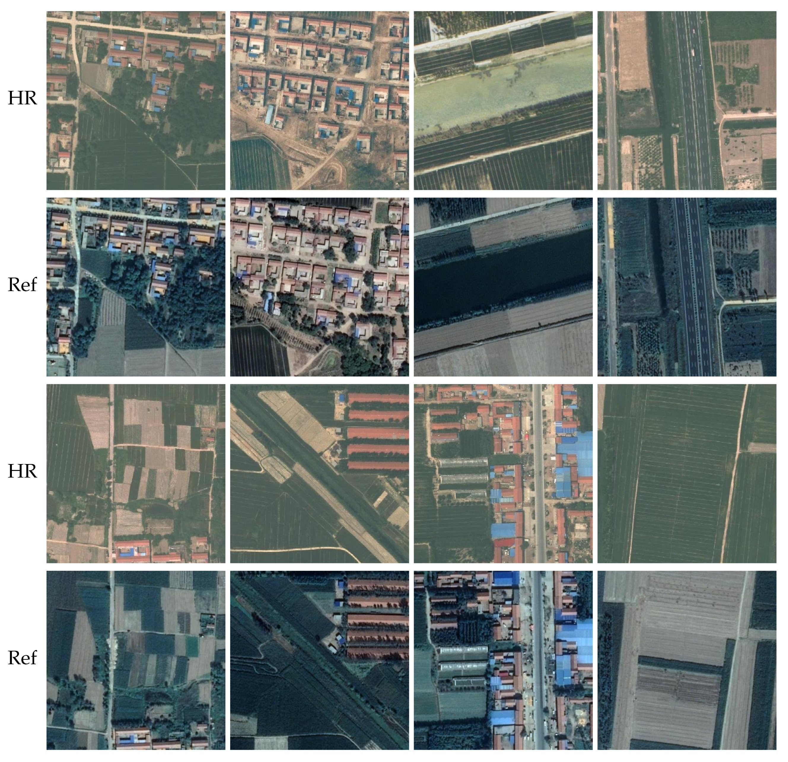
30] as the training set, which consists of 4047 pairs of HR-Ref images with RGB bands, including common remote sensing scenes such as airports, farmlands, and ports. HR images were chosen from WorldView-2 and GaoFen-2 datasets, while Ref images were searched in Google Earth, in compliance with the horizontal and vertical coordinates of remote sensing images. HR and Ref images were 480 × 480 pixels in size, while LR images had a size of 120 × 120. In this paper, the HR image was downsampled four times to obtain the corresponding LR image.
Figure 4 displays an example training set, including HR-Ref image pairs.
Testing Dataset. RRSSRD contained four test datasets, each consisting of 40 pairs of HR-Ref images. The first two test sets depict Xiamen city with different spatial resolutions in different periods, and the last two datasets are Jinan city with different spatial resolutions in different periods. The Ref images in the test set were also collected from Google Earth.
Implementation Details. A total of 135 image pairs in the aforementioned RRSSRD were randomly selected as the validation dataset, and the rest were used for training at a
scaling factor. Actually, the first three feature maps extracted from a pretrained FEE were utilized as the basis of feature exchange. To improve the matching efficiency, only the third layer was matched, and then the corresponding relationship was directly mapped to the first layer and the second layer, so that all layers used the same corresponding relationship. The parameter setting during the training process was displayed in
Table 2. The training model adopted an ADAM optimizer [
34] with
and
. We set the learning rate and the batch size to
and 6. For the loss hyperparameters, we set
,
, and
to 1,
and
. At first, only five epochs were pretrained; then, 100 epochs were trained. To reinforce the generalization facility of the model, we regularized the train set by random horizontal and vertical flipping, followed by random rotations by 90°, 180°, and 270°.
4.2. Qualitative Evaluation
In this section, we used the proposed method and nine comparison methods to reconstruct the remote sensing reference images on four test sets. The nine comparison methods were Bicubic [
35], SRResNet [
19], MDSR [
36], WDSR [
15], ESRGAN [
20], SPSR [
21], CrossNet [
27], SRNTT [
28], and RRSGAN [
30]. Among them, Bicubic, SRResNet, MDSR, WDSR, ESRGAN, and SPSR are image super-resolution reconstruction methods without reference images, and the remaining three are RefSR methods. To obtain a fair comparison, all models were trained on RRSSRD, and all the result graphs were scaled to the same proportion for convenient comparison.
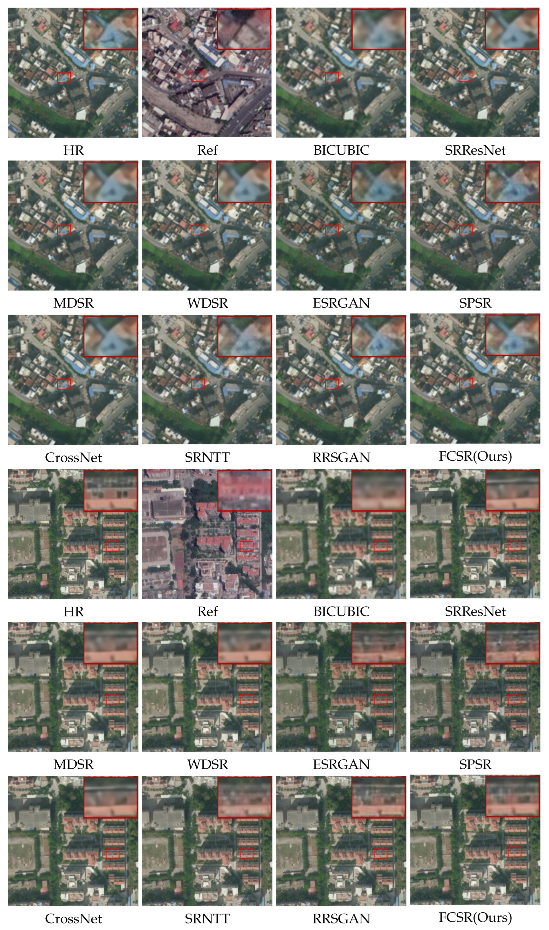
Figure 5 presents a visual comparison of our proposed model and other SISR methods and RefSR methods, focusing on two remote sensing images. The results of Bicubic interpolation lack details that are beneficial to image reconstruction. CNN-based SR methods, such as SRResNet, MDSR and WDSR, can reconstruct some texture details of remote sensing images, but there is still the problem of blurred contours due to the shortage of optimized objective functions. GAN-based SR methods, such as ESRGAN and SPSR, have better visual details, but produce artifacts, resulting in poor reconstruction results. Due to the inherent properties of the patch matching method, there are blocky artifacts in the SR results of SRNTT. Compared with other SR methods, our FCSR method can transfer more accurate HR textures from the reference image, recover more texture details, avoid introducing artifacts as much as possible, and make the remote sensing image reconstruction results more natural and true. For instance, in the first example in
Figure 5, SRRestNet, WDSR, and MDSR present blurry details of the building, while the SPSR results produce obvious distortions. Meanwhile, our proposed FCSR reconstructs more natural details.
4.3. Quantitative Evaluation
In addition to qualitative analysis, we use two objective evaluation indexes, peak signal-to-noise ratio (PSNR) [
37] and structural similarity (SSIM) [
38], which are commonly used in image processing to evaluate the image reconstruction effect. PSNR was calculated based on the error between corresponding pixels in the image. The larger the calculated value, the lower the rate of distortion and the better the restoration effect. SSIM measured image similarity from three aspects: brightness, contrast, and structure. The value range was 0–1. Similarly, a larger SSIM value means less distortion and a better image restoration effect.
Table 3 shows the quantitative comparison results for the images of nine comparison methods, as shown in
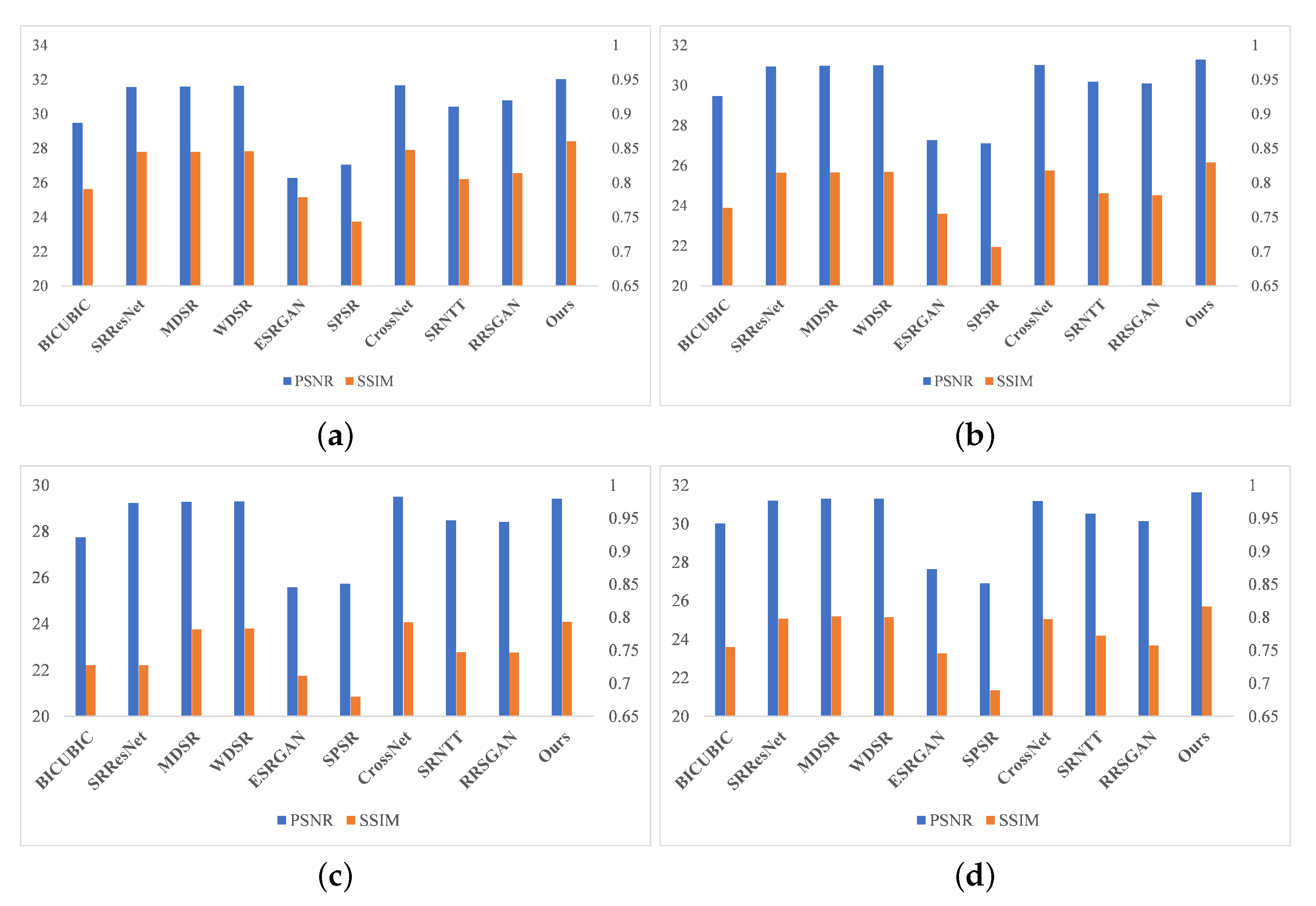
Figure 5, and the images of our proposed method. Red represents the best result and blue represents the second-best result. The table shows that WDSR achieved the best results in terms of PSNR and SSIM indicators during the comparison of six SR methods. The method in this paper achieved the best results in four test sets, and is more advantageous than the latest SR method and Ref-SR method, even when comparing these methods in an attempt to obtain better visual quality with adversarial loss. Compared with the optimal value of the comparison methods, the proposed method in this paper has an average PSNR value of 1.0877% and an average SSIM value that is 1.4764% higher in the first test set; an average PSNR value of 0.8161% and an average SSIM value that is 1.4467% higher in the second test set; an average SSIM value that is 0.0882% higher in the third test set; an average PSNR value of 1.0296%; and an average SSIM value that is 1.8371% higher in the fourth test set. The quantitative results show that our FCSR method is superior to other super-resolution methods. The visualization results for the average PSNR and SSIM values are depicted in
Figure 6. The PSNR and SSIM of FCSR on the test sets are superior to the others, demonstrating the effectiveness of our method.
5. Discussion
In this section, we verified the necessity of the key parts of the network proposed in this paper, namely, FCB and FEE, by conducting ablation experiments on different models. Meanwhile, the limitations of FCSR were analyzed.
5.1. Effectiveness of FCB
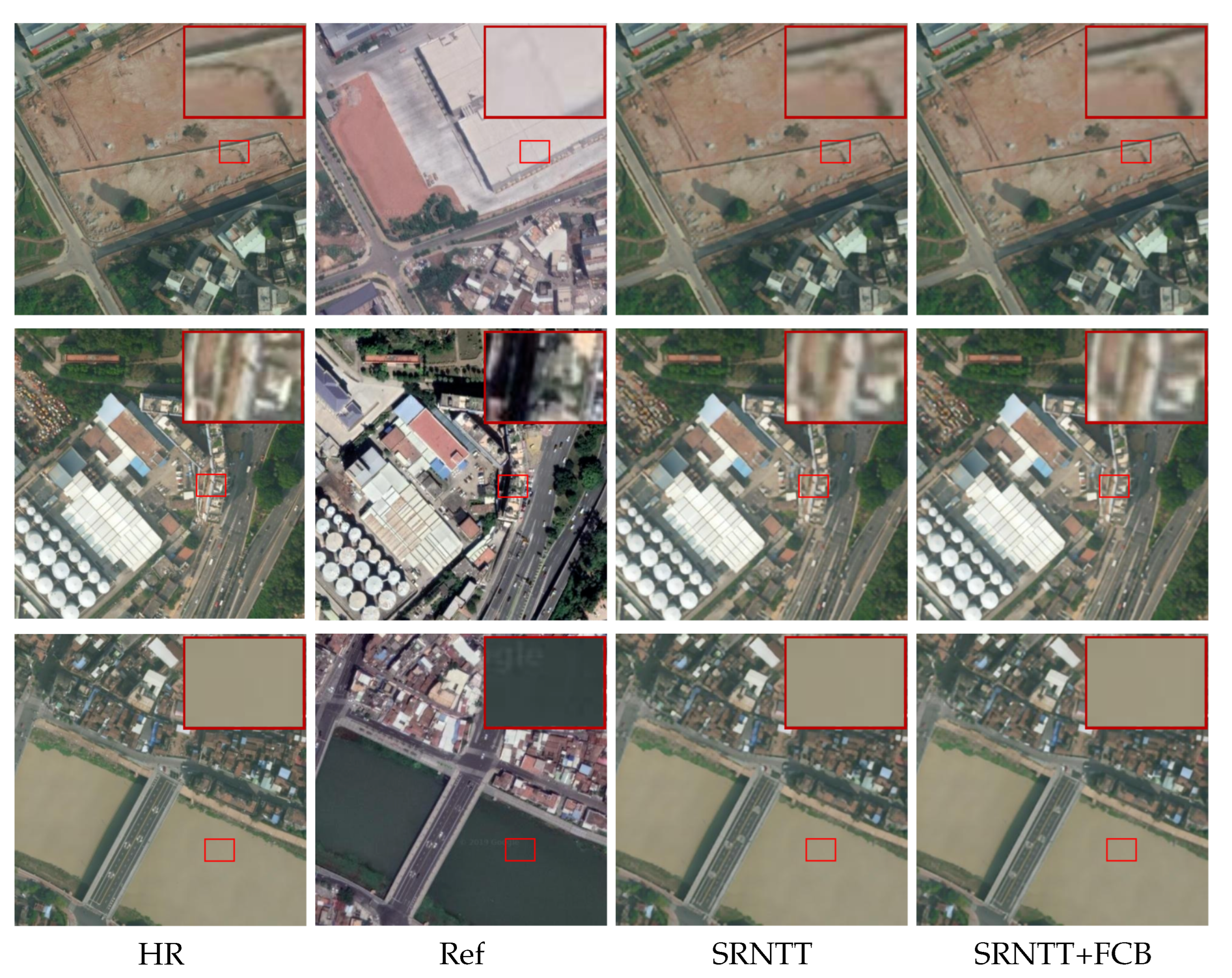
To verify the key role that FCB plays in feature matching and exchange between LR and Ref images, FCB was added without varying the structure of other parts of SRNTT. The results in the first and second columns of
Table 4 separately show the average PSNR and SSIM values of SRNTT and SRNTT+FCB reconstruction results on four identical test sets. Compared with SRNTT, SRNTT+FCB increased the PSNR and SSIM values by 1.53 dB and 6.5553%, respectively, on the first test set, 1.03 dB and 5.5950%, respectively, on the second test set, 0.90 dB and 6.1888% on the third test set, and 0.98 dB and 5.4236% on the fourth test set. As shown in
Figure 7, the generated image quality with FCB is preferable regrading feature details and hue.
5.2. Effectiveness of FEE
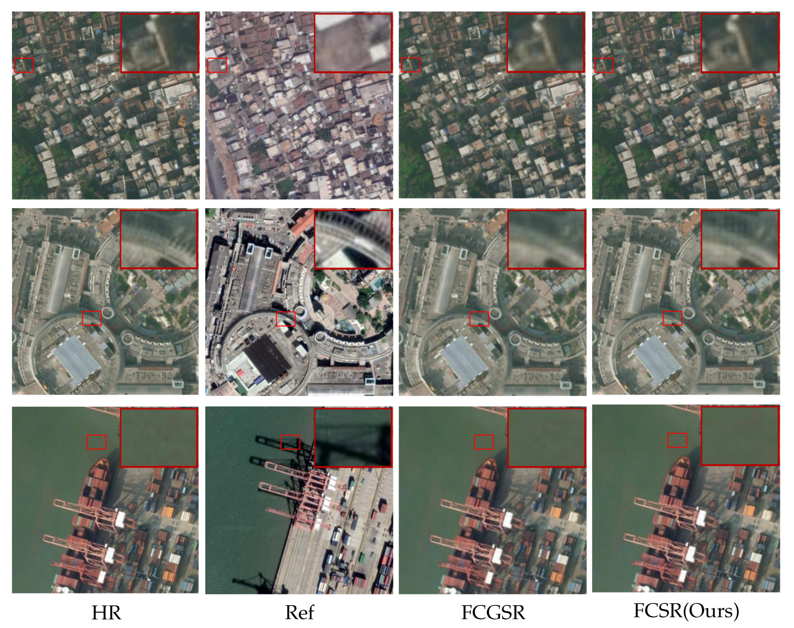
To demonstrate the effectiveness of FEE in feature extraction from LR and Ref images, on the condition of keeping the structure of other parts of the FCSR constant, the FEE used for feature extraction was replaced by VGG19. Thus, FCB became FCG. We named the new network FCGSR. The results in the third and fourth columns in
Table 4 show the average PSNR and SSIM values of the reconstruction results of FCGSR and FCSR in this paper when tested on four identical test sets. Specifically, compared with the FCGSR, the FCSR increases the PSNR and SSIM values by 0.17 dB and 0.7556% on the first test set, 0.09 dB and 0.5546% on the second test set, 0.04 dB and 0.2899% on the third test set, and 0.06 dB and 0.3062% on the fourth test set. As presented in
Figure 8, the reconstruction results are superior regarding texture details.
5.3. Hyperparameter Tuning of SVD Coefficients
We carried out ablation experiments to understand the impact of the different SVD coefficients described in
Section 3.1 Feature Compression Branch. We used the same training strategy and network parameters that were introduced in
Table 4 while adjusting the values of SVD coefficients
,
a, and
b. To verify that the setting of the SVD coefficients is appropriate, as a singular values ratio larger than 0.2 is a waste of the source, we experiment with seven sets of parameters. As shown in
Table 2, we first explored the effect of adjusting only the ratio of singular values taken at
a and
b with a consistent
in the four lines. Compared to the performance of these four methods presented in
Table 5, the proposed method shows an obvious improvement, with a PSNR of 0.094 dB on average for the four test sets compared to the suboptimal setting. When setting the cosine similarity criterion, we utilized three values: 0.75, 0.80, and 0.85. Quantitative comparisons show that FCSR is superior to the three methods, with a PSNR improvement of 0.025 dB, on average, for the four test sets compared to the suboptimal setting. To achieve the best performance, we set the weight hyperparameters for
,
a, and
b as 0.88, 0.1, and 0.2, respectively.
5.4. Hyperparameter Tuning of Loss Weight
We conducted ablation experiments to prove the impact of different loss terms. The same training strategy and network parameters that were introduced in
Table 2 were reserved in the following experiments, except for the different loss weights. To determine a suitable setting for the loss weights, based on the commonly used loss weights in the SR methods, we implemented three sets of hyperparameters. Following the setting of different loss weights in [
28], we set
to 1. First, we experimented with the effect of only using reconstruction loss
, when
and
were set to 0. The following experiments adjusted
and
to
. As shown in
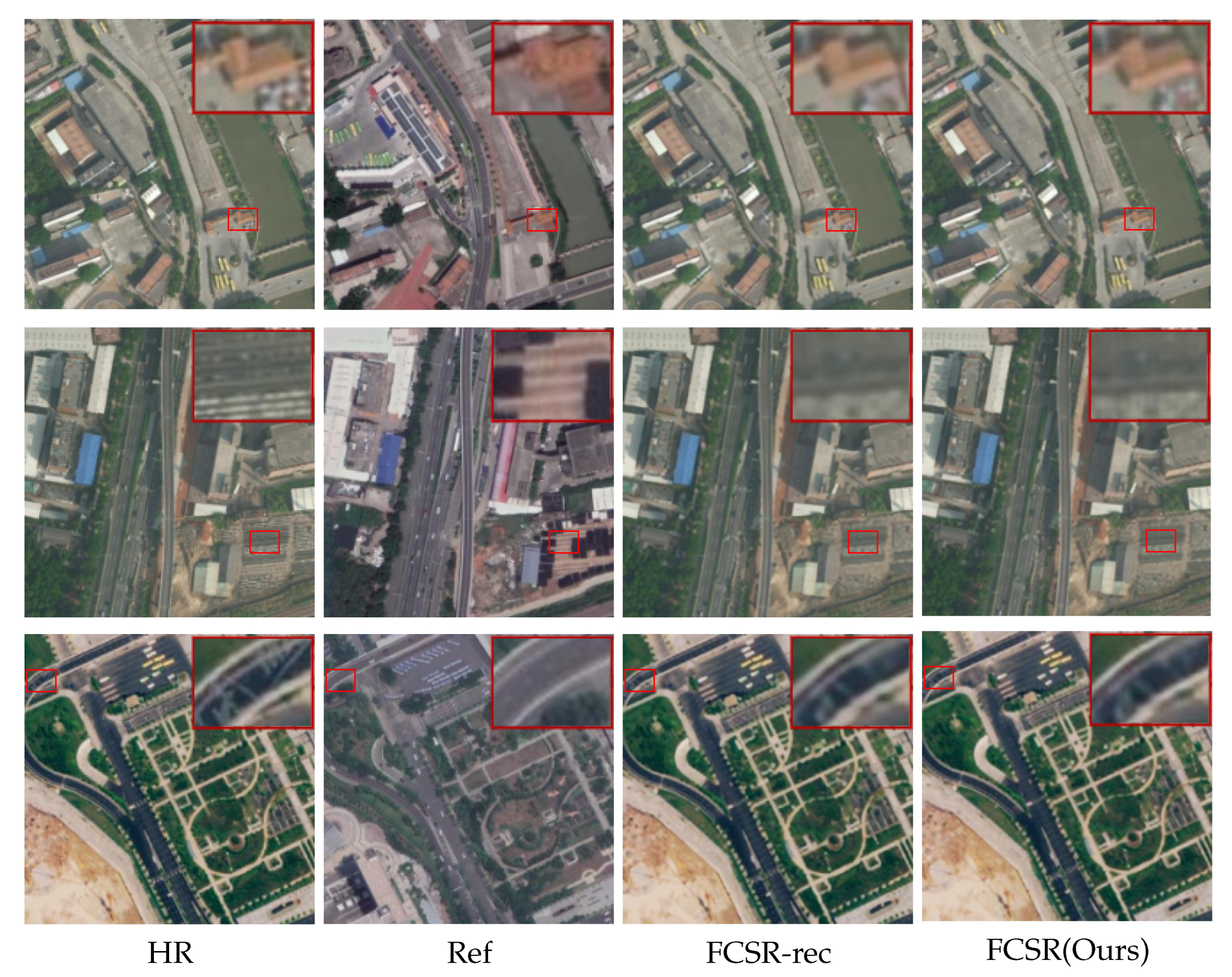
Table 6, the highest PSRN and SSIM values can be obtained only using reconstruction loss compared with other loss weight settings. However, the reconstruction loss function often leads to overly smoothed results and is weak in reconstructing natural texture details. The introduction of the perceptual loss
and adversarial loss
can greatly improve the visual quality of reconstruction, which has been verified in
Figure 9. With perceptual loss
and adversarial loss
, our proposed method recovers more details than FCSR-rec, which implies only using reconstruction loss when training FCSR.
Meanwhile, excessive adversarial loss and perceptual loss weights can reduce the performance of the SR results. As shown in
Table 6, our method improves PSNR with 1.710 dB on average for the four test sets compared to only increasing
. Additionally, the improvement of PSNR on average for the four test sets over only increasing
is 0.110 dB. In such a situation, the reconstruction loss can provide clearer guidance of texture transfer than the adversarial loss and the perceptual loss. To balance the image reconstruction effect and image quality, we set the weight hyperparameters for
,
, and
to 1,
and
, respectively.
5.5. Model Efficiency
As depicted in
Table 7, we reported the values of the model parameters and the computational complexity of eight different image super-resolution methods. The model parameter values of the proposed method is smaller than those of RefSR methods such as CrossNet and RRSGAN. Meanwhile, model parameters are even lower than DBPN, ESRGAN, and SPSR, which do not utilize reference images. The video memory footprint, to some extent, can reduce the time of program initialization. Additionally, a lower number of network parameters prevent overfitting during the training process. However, models with more parameters have a better memory. In other words, our proposed model has a limited learning ability, which increases the difficulty of training to a certain extent. Due to the continuous accumulation of feature maps and the growth in memory access costs, the computational complexity of the proposed method is large. There is no doubt that this vast computational complexity leads to a longer training time. In future studies, we will further optimize the training efficiency of our proposed model.
5.6. Limitations
Using an abundance of qualitative and quantitative experiments, it was adequately confirmed that our proposed FCSR has the best subjective and objective results in test sets; nonetheless, this method still has limitations. When the quality of the remote sensing image is lower and the image cannot be magnified more than four times, this method does not propose corresponding solutions, and more researches need to be conducted. Meanwhile, this method requires a remote sensing image in the same longitude and latitude position in different time frames, which can be used as an HR and Ref image. This means that datasets have strict requirements, and promotes the feature extraction of remote sensing image pairs, making the method more broadly applicable.
6. Conclusions
Due to the large-scale variability, the complexity of scenes, and the fine structures of objects, we propose a new, reference-based, super-resolution reconstruction method named FCSR for remote sensing images, focusing on three aspects. First, this method takes full advantage of the internal longitude and latitude information of remote sensing images, which can adequately accomplish feature extraction, matching and exchanging between the LR and Ref images. Synchronously, this information is attached to a subsequent texture transfer module, furnishing information replenishment for the LR image and providing a new method for the super-resolution reconstruction of remote sensing images. Second, the designed FCB introduces the SVD algorithm in machine learning to remote sensing image compression, performs sparse feature processing on LR images and corresponding Ref images, and screens out redundant information in the images; thus, the remaining information complements the context features that are lacking in remote sensing images via feature extraction, matching, and exchange modules. Third, because the VGG19 trained by natural images is not suitable for the feature extraction of remote sensing images, FEE was designed to obtain the multi-level features of remote sensing image pairs, improve the extent of matching between the LR remote sensing image and the corresponding Ref image, and effectively intensify the parallel features contained in image pairs. When subject to qualitative and quantitative analysis, the proposed FCSR shows the strong competitiveness in the super-resolution reconstruction of remote sensing images. The high-quality remote sensing images derived by FCSR can be further applied in the fields of ecological indicators mapping, urban-rural management, water resource management, hydrological models, wastewater treatment, water pollution, and urban planning. In future studies, we will explore the following obstacles. First, we will optimize the training efficiency of our proposed model. Second, we will exploit a new method to match reference images that have temporal, scale, and angle differences compared to HR images. Third, we will attempt to introduce RefSR to broadband images to increase the availability of the proposed method. Last but not least, we will apply the proposed method to low-resolution remote sensing images to meet the needs of more subsequent tasks.
Author Contributions
Conceptualization, B.J. and L.W.; methodology, J.Z. and X.C.; software, J.Z. and X.C.; validation, X.C., X.T. and K.C.; data curation, J.Z.; writing—original draft preparation, J.Z., B.J. and J.J.; writing—review and editing, J.Z., X.C., K.C. and Y.Y.; supervision, W.Z., B.J. and X.C. All authors have read and agreed to the published version of the manuscript.
Funding
This research is supported by the National Natural Science Foundation of China (Nos. 42271140 and 61801384), the National Key Research and Development Program of China (No. 2019YFC1510503), the Natural Science Basic Research Program of Shaanxi Province of China (No. 2017JQ4003), and the Key Research and Development Program of Shaanxi Province of China (Nos. 2021KW-05, 2023-YBGY-242, and 2020KW-010).
Data Availability Statement
The data of experimental images used to support the findings of this research are available from the corresponding author upon reasonable request.
Conflicts of Interest
All authors declare no conflicts of interest.
Abbreviations
The following abbreviations are used in this paper:
| SR | Super-resolution |
| LR | Low-resolution |
| HR | High-resolution |
| Ref | Reference |
| RefSR | Reference-based super-resolution |
| PSNR | Peak signal-to-noise ratio |
| SSIM | Structural similarity |
| CNN | Convolutional neural network |
| FCB | Feature compression branch |
| FCM | Feature compression module |
| FEE | Feature extraction encoder |
References
- Xia, G.S.; Yang, W.; Delon, J.; Gousseau, Y.; Hong, S. Structural High-resolution Satellite Image Indexing. In Proceedings of the ISPRS TC VII Symposium—100 Years ISPRS, Vienna, Austria, 5–7 July 2010. [Google Scholar]
- Yüksel, M.; Kucuk, S.; Yuksel, S.; Erdem, E. Deep Learning for Medicine and Remote Sensing: A Brief Review. Int. J. Environ. Geoinformatics 2020, 7, 280–288. [Google Scholar] [CrossRef]
- Sumbul, G.; Demir, B. A Deep Multi-Attention Driven Approach for Multi-Label Remote Sensing Image Classification. IEEE Access 2020, 8, 95934–95946. [Google Scholar] [CrossRef]
- Yuan, Q.; Shen, H.; Li, T.; Li, Z.; Li, S.; Jiang, Y.; Xu, H.; Tan, W.; Yang, Q.; Wang, J.; et al. Deep learning in environmental remote sensing: Achievements and challenges. Remote Sens. Environ. 2020, 241, 111716. [Google Scholar] [CrossRef]
- Fernandez-Beltran, R.; Latorre-Carmona, P.; Pla, F. Single-frame super-resolution in remote sensing: A practical overview. Int. J. Remote Sens. 2017, 38, 314–354. [Google Scholar] [CrossRef]
- Lei, S.; Shi, Z.; Zou, Z. Coupled Adversarial Training for Remote Sensing Image Super-Resolution. IEEE Trans. Geosci. Remote. Sens. 2020, 58, 3633–3643. [Google Scholar] [CrossRef]
- Dong, C.; Loy, C.C.; He, K.; Tang, X. Image Super-Resolution Using Deep Convolutional Networks. IEEE Trans. Pattern Anal. Mach. Intell. 2016, 38, 295–307. [Google Scholar] [CrossRef]
- Zhang, L.; Zhang, L.; Du, B. Deep Learning for Remote Sensing Data: A Technical Tutorial on the State of the Art. IEEE Geosci. Remote Sens. Mag. 2016, 4, 22–40. [Google Scholar] [CrossRef]
- Liu, Z.S.; Siu, W.C.; Chan, Y.L. Reference Based Face Super-Resolution. IEEE Access 2019, 7, 129112–129126. [Google Scholar] [CrossRef]
- Dong, C.; Loy, C.C.; He, K.; Tang, X. Learning a Deep Convolutional Network for Image Super-Resolution. In Proceedings of the European Conference on Computer Vision(ECCV), Zurich, Switzerland, 6–12 September 2014; pp. 184–199. [Google Scholar]
- Warbhe, S.; Gomes, J. Interpolation Technique using Non Linear Partial Differential Equation with Edge Directed Bicubic. Int. J. Image. Processing 2016, 10, 205–213. [Google Scholar]
- Balashov, M.V. On the gradient projection method for weakly convex functions on a proximally smooth set. Math. Notes 2020, 108, 643–651. [Google Scholar] [CrossRef]
- Chang, H.; Yeung, D.Y.; Xiong, Y. Super-resolution through neighbor embedding. In Proceedings of the 2004 IEEE Computer Society Conference on Computer Vision and Pattern Recognition, 2004. CVPR 2004, Washington, DC, USA, 27 June–2 July 2004. [Google Scholar]
- Yang, J.; Wright, J.; Huang, T.S.; Ma, Y. Image super-resolution as sparse representation of raw image patches. In Proceedings of the 2008 IEEE Conference on Computer Vision and Pattern Recognition, Anchorage, AK, USA, 23–28 June 2008; pp. 1–8. [Google Scholar]
- Yu, J.; Fan, Y.; Yang, J.; Xu, N.; Wang, Z.; Wang, X.; Huang, T.S. Wide Activation for Efficient and Accurate Image Super-Resolution. arXiv 2018, arXiv:1808.08718. [Google Scholar]
- Kim, J.; Lee, J.K.; Lee, K.M. Accurate Image Super-Resolution Using Very Deep Convolutional Networks. In Proceedings of the 2016 IEEE Conference on Computer Vision and Pattern Recognition (CVPR), Las Vegas, NV, USA, 27–30 June 2016; pp. 1646–1654. [Google Scholar]
- He, K.; Zhang, X.; Ren, S.; Sun, J. Deep Residual Learning for Image Recognition. In Proceedings of the 2016 IEEE Conference on Computer Vision and Pattern Recognition (CVPR), Las Vegas, NV, USA, 27–30 June 2016; pp. 770–778. [Google Scholar] [CrossRef]
- Goodfellow, I.J.; Pouget-Abadie, J.; Mirza, M.; Xu, B.; Warde-Farley, D.; Ozair, S.; Courville, A.C.; Bengio, Y. Generative Adversarial Nets. In Proceedings of the 2014 27th International Conference on Neural Information Processing Systems(NIPS)-Volume 2, Cambridge, MA, USA, 8–13 December 2014; pp. 2672–2680. [Google Scholar]
- Ledig, C.; Theis, L.; Huszár, F.; Caballero, J.; Cunningham, A.; Acosta, A.; Aitken, A.; Tejani, A.; Totz, J.; Wang, Z.; et al. Photo-Realistic Single Image Super-Resolution Using a Generative Adversarial Network. In Proceedings of the 2017 IEEE Conference on Computer Vision and Pattern Recognition (CVPR), Honolulu, HI, USA, 21–26 July 2017; pp. 105–114. [Google Scholar] [CrossRef]
- Wang, X.; Yu, K.; Wu, S.; Gu, J.; Liu, Y.; Dong, C.; Loy, C.C.; Qiao, Y.; Tang, X. ESRGAN: Enhanced Super-Resolution Generative Adversarial Networks. In Proceedings of the European Conference on Computer Vision(ECCVW), Munich, Germany, 8–14 September 2018; pp. 63–79. [Google Scholar]
- Ma, C.; Rao, Y.; Cheng, Y.; Chen, C.; Lu, J.; Zhou, J. Structure-Preserving Super Resolution With Gradient Guidance. In Proceedings of the 2020 IEEE/CVF Conference on Computer Vision and Pattern Recognition (CVPR), Seattle, WA, USA, 13–19 June 2020; pp. 7766–7775. [Google Scholar]
- Wang, X.; Wu, Y.; Ming, Y.; Lv, H. Remote Sensing Imagery Super Resolution Based on Adaptive Multi-Scale Feature Fusion Network. Sensors 2020, 20, 1142. [Google Scholar] [CrossRef] [PubMed]
- Xu, W.; Xu, G.; Wang, Y.; Sun, X.; Lin, D.; Wu, Y. High Quality Remote Sensing Image Super-Resolution Using Deep Memory Connected Network. In Proceedings of the IGARSS 2018—2018 IEEE International Geoscience and Remote Sensing Symposium, Valencia, Spain, 22–27 July 2018; pp. 8889–8892. [Google Scholar]
- po Ma, W.; Pan, Z.; Guo, J.; Lei, B. Achieving Super-Resolution Remote Sensing Images via the Wavelet Transform Combined With the Recursive Res-Net. IEEE Trans. Geosci. Remote Sens. 2019, 57, 3512–3527. [Google Scholar]
- Boominathan, V.; Mitra, K.; Veeraraghavan, A. Improving resolution and depth-of-field of light field cameras using a hybrid imaging system. In Proceedings of the 2014 IEEE International Conference on Computational Photography (ICCP), Santa Clara, CA, USA, 2–4 May 2014; pp. 1–10. [Google Scholar]
- Yue, H.; Sun, X.; Yang, J.; Wu, F. Landmark Image Super-Resolution by Retrieving Web Images. IEEE Trans. Image Process. 2013, 22, 4865–4878. [Google Scholar] [PubMed]
- Zheng, H.; Ji, M.; Wang, H.; Liu, Y.; Fang, L. CrossNet: An End-to-end Reference-based Super Resolution Network using Cross-scale Warping. In Proceedings of the European Conference on Computer Vision, Munich, Germany, 8–14 September 2018. [Google Scholar]
- Zhang, Z.; Wang, Z.; Lin, Z.L.; Qi, H. Image Super-Resolution by Neural Texture Transfer. In Proceedings of the 2019 IEEE/CVF Conference on Computer Vision and Pattern Recognition (CVPR), Long Beach, CA, USA, 16–20 June 2019; pp. 7974–7983. [Google Scholar]
- Simonyan, K.; Zisserman, A. Very Deep Convolutional Networks for Large-Scale Image Recognition. arXiv 2014, arXiv:1409.1556. [Google Scholar]
- Dong, R.; Zhang, L.; Fu, H. RRSGAN: Reference-Based Super-Resolution for Remote Sensing Image. IEEE Trans. Geosci. Remote Sens. 2022, 60, 1–17. [Google Scholar] [CrossRef]
- Leibovici, D.G.; Sabatier, R. A singular value decomposition of a k-way array for a principal component analysis of multiway data, PTA-k. Linear Algebra Its Appl. 1998, 269, 307–329. [Google Scholar] [CrossRef]
- Ronneberger, O.; Fischer, P.; Brox, T. U-Net: Convolutional Networks for Biomedical Image Segmentation. In Proceedings of the 2015 18th International Conference on Medical Image Computing and Computer-Assisted Intervention(MICCAI), Munich, Germany, 5–9 October 2015; pp. 234–241. [Google Scholar]
- Gulrajani, I.; Ahmed, F.; Arjovsky, M.; Dumoulin, V.; Courville, A.C. Improved Training of Wasserstein GANs. In Proceedings of the the 2017 31st International Conference on Neural Information Processing Systems(NIPS), Long Beach, CA, USA, 4–9 December 2017; pp. 5769–5779. [Google Scholar]
- Kingma, D.; Ba, J. Adam: A Method for Stochastic Optimization. arXiv 2014, arXiv:1412.6980. [Google Scholar]
- Keys, R. Cubic convolution interpolation for digital image processing. IEEE Trans. Acoust. Speech, Signal Process. 1981, 29, 1153–1160. [Google Scholar] [CrossRef]
- Lim, B.; Son, S.; Kim, H.; Nah, S.; Lee, K.M. Enhanced Deep Residual Networks for Single Image Super-Resolution. In Proceedings of the 2017 IEEE Conference on Computer Vision and Pattern Recognition Workshops (CVPRW), Honolulu, HI, USA, 21–26 July 2017; pp. 1132–1140. [Google Scholar]
- Horé, A.; Ziou, D. Image Quality Metrics: PSNR vs. SSIM. In Proceedings of the 2010 20th International Conference on Pattern Recognition, Istanbul, Turkey, 23–26 August 2010; pp. 2366–2369. [Google Scholar] [CrossRef]
- Wang, Z.; Bovik, A.C.; Sheikh, H.R.; Simoncelli, E.P. Image quality assessment: From error visibility to structural similarity. IEEE Trans. Image Process. 2004, 13, 600–612. [Google Scholar] [CrossRef] [PubMed]
Figure 1.
Overall framework of our FCSR method. This consists of three components: content extractor, similar feature acquisition, and texture transfer. Similar feature acquisition provided supplementary information according to the feature premise, and the matching and exchange between the LR and Ref image occurred to ensure texture transfer and reconstruct SR images.
Figure 2.
The architecture of the proposed modules. (a) texture swapping branch; (b) feature compression branch (FCB). The FCB is composed of a feature compression module (FCM) and texture swapping branch. FCM employs SVD to adaptively offer complementary information between the LR and Ref images. The texture swapping branch furnishes multi-level features, which are displayed as Level 1 features, Level 2 features, and Level 3 features.
Figure 3.
The structure of a multi-level self-encoder. FEE is the coding portion of the multi-level self-encoder. When pretrained with remote sensing images, FEE is prone to extracting appropriately similar features from the LR and Ref images.
Figure 3.
The structure of a multi-level self-encoder. FEE is the coding portion of the multi-level self-encoder. When pretrained with remote sensing images, FEE is prone to extracting appropriately similar features from the LR and Ref images.
Figure 4.
Examples of RRSSRD training set. The first and third rows represent HR images while the second and fourth rows represent Ref images. Specifically, HR images in the first row correspond to Ref images in the second row, and HR images in the third row correspond to Ref images in the fourth row.
Figure 5.
Visual comparison of some typical SR methods and our model of ×4 factor on the first test set. The results of comparison methods originate from [
30]. We enlarge the image details inside the light red rectangle and show in the red rectangle in the upper right corner.
Figure 5.
Visual comparison of some typical SR methods and our model of ×4 factor on the first test set. The results of comparison methods originate from [
30]. We enlarge the image details inside the light red rectangle and show in the red rectangle in the upper right corner.
Figure 6.
Visualization results of average PSNR and SSIM values for diverse SR methods of ×4 factor. (a) PSNR and SSIM on 1st test set; (b) PSNR and SSIM on 2nd test set; (c) PSNR and SSIM on 3rd test set; (d) PSNR and SSIM on 4th test set.
Figure 6.
Visualization results of average PSNR and SSIM values for diverse SR methods of ×4 factor. (a) PSNR and SSIM on 1st test set; (b) PSNR and SSIM on 2nd test set; (c) PSNR and SSIM on 3rd test set; (d) PSNR and SSIM on 4th test set.
Figure 7.
Visual comparison between SRNTT and SRNTT+FCB of ×4 factor on diverse test sets. We enlarge the image details inside the light red rectangle and show in the red rectangle in the upper right corner.
Figure 7.
Visual comparison between SRNTT and SRNTT+FCB of ×4 factor on diverse test sets. We enlarge the image details inside the light red rectangle and show in the red rectangle in the upper right corner.
Figure 8.
Visual comparison between FCGSR and our FCSR method of ×4 factor on various test sets. We enlarge the image details inside the light red rectangle and show in the red rectangle in the upper right corner.
Figure 8.
Visual comparison between FCGSR and our FCSR method of ×4 factor on various test sets. We enlarge the image details inside the light red rectangle and show in the red rectangle in the upper right corner.
Figure 9.
Visual comparison between FCSR-rec and the proposed method of ×4 factor on diverse test sets. FCSR-rec denotes only using reconstruction loss when training FCSR. We enlarge the image details inside the light red rectangle and show in the red rectangle in the upper right corner.
Figure 9.
Visual comparison between FCSR-rec and the proposed method of ×4 factor on diverse test sets. FCSR-rec denotes only using reconstruction loss when training FCSR. We enlarge the image details inside the light red rectangle and show in the red rectangle in the upper right corner.
Table 1.
Detailed network parameter settings of FEE, where H and W imply the height and width of the feature map, while C denotes the channel number. In this table, Res-block-1 and Res-block-2 are parts of Res-blocks. FEE is composed of 3 Res-blocks, 4 Res-blocks, and 6 Res-blocks.
Table 1.
Detailed network parameter settings of FEE, where H and W imply the height and width of the feature map, while C denotes the channel number. In this table, Res-block-1 and Res-block-2 are parts of Res-blocks. FEE is composed of 3 Res-blocks, 4 Res-blocks, and 6 Res-blocks.
| Structure Component | Layer | Input | Output |
|---|
| Res-block-1 | Conv3×3 | | |
| Relu | | |
| Conv | | |
| Relu | | |
| Res-block-2 | Conv3×3 | | |
| Relu | | |
| Conv | | |
| Relu | | |
| 3 Res-blocks | Res-block-1 | | |
| Res-block-2 × 2 | | |
| Maxpool | | |
| 4 Res-blocks | Res-block-1 | | |
| Res-block-2 × 3 | | |
| Maxpool | | |
| 6 Res-blocks | Res-block-1 | | |
| Res-block-2 × 5 | | |
| Maxpool | | |
Table 2.
Parameter setting during the training process.
Table 2.
Parameter setting during the training process.
| Parameters | Setting |
|---|
| Batch size | 6 |
| Training epoch number | 100 |
| Optimization method | Adam [35], , |
| Loss hyperparameters | |
Table 3.
Average PSNR and SSIM results of various SR methods of ×4 factor on the four test sets. Red index denotes the best performance. Blue index suggests suboptimal performance. The results of these comparison methods originate from [
30].
Table 3.
Average PSNR and SSIM results of various SR methods of ×4 factor on the four test sets. Red index denotes the best performance. Blue index suggests suboptimal performance. The results of these comparison methods originate from [
30].
| Dataset | Metrics | BICUBIC | SRResNet | MDSR | WDSR | ESRGAN |
|---|
1st
testset | PSNR | 29.4836 | 31.5690 | 31.5913 | 31.6308 | 26.2821 |
| SSIM | 0.7908 | 0.8448 | 0.8448 | 0.8456 | 0.7788 |
2nd
testset | PSNR | 29.4625 | 30.9378 | 30.9672 | 31.0029 | 27.2674 |
| SSIM | 0.7636 | 0.8146 | 0.8148 | 0.8158 | 0.7549 |
3rd
testset | PSNR | 27.7488 | 29.2300 | 29.2853 | 29.3005 | 25.5791 |
| SSIM | 0.7275 | 0.7275 | 0.7822 | 0.7827 | 0.7112 |
4th
testset | PSNR | 30.0147 | 31.2072 | 31.3084 | 31.2988 | 27.6430 |
| SSIM | 0.7546 | 0.7981 | 0.8015 | 0.8003 | 0.7456 |
| Dataset | Metrics | SPSR | CrossNet | SRNTT | RRSGAN | Ours |
1st
testset | PSNR | 27.0478 | 31.6646 | 30.4134 | 30.7872 | 32.0128 |
| SSIM | 0.7435 | 0.8475 | 0.8054 | 0.8141 | 0.8602 |
2nd
testset | PSNR | 27.0927 | 31.0160 | 30.1791 | 30.0951 | 31.2712 |
| SSIM | 0.7066 | 0.8175 | 0.7846 | 0.7816 | 0.8295 |
3rd
testset | PSNR | 25.7461 | 29.4988 | 28.4779 | 28.4161 | 29.4156 |
| SSIM | 0.6800 | 0.7926 | 0.7473 | 0.7464 | 0.7933 |
4th
testset | PSNR | 26.9183 | 31.1849 | 30.5349 | 30.1492 | 31.6341 |
| SSIM | 0.6897 | 0.7975 | 0.7725 | 0.7576 | 0.8165 |
Table 4.
Average PSNR and SSIM results for four different models of ×4 factor on four test sets.
Table 4.
Average PSNR and SSIM results for four different models of ×4 factor on four test sets.
| Dataset | Metrics | SRNTT | SRNTT+FCB | FCGSR | OURS |
|---|
1st
testset | PSNR | 30.4134 | 31.9430 | 31.8417 | 32.0128 |
| SSIM | 0.8054 | 0.8619 | 0.8537 | 0.8602 |
2nd
testset | PSNR | 30.1791 | 31.2002 | 31.1857 | 31.2712 |
| SSIM | 0.7846 | 0.8311 | 0.8249 | 0.8295 |
3rd
testset | PSNR | 28.4779 | 29.3764 | 29.3733 | 29.4156 |
| SSIM | 0.7473 | 0.7966 | 0.7910 | 0.7933 |
4th
testset | PSNR | 30.5349 | 31.5113 | 31.5734 | 31.6341 |
| SSIM | 0.7725 | 0.8168 | 0.8140 | 0.8165 |
Table 5.
Results of average PSNR and SSIM results of different SVD coefficients on four test sets. Red index denotes the best performance. Blue index suggests the suboptimal performance for adjusting a and b. Purple index suggests the suboptimal performance for adjusting .
Table 5.
Results of average PSNR and SSIM results of different SVD coefficients on four test sets. Red index denotes the best performance. Blue index suggests the suboptimal performance for adjusting a and b. Purple index suggests the suboptimal performance for adjusting .
| Dataset | 1st Testset | 2nd Testset | 3rd Testset | 4th Testset |
|---|
| Metrics | PSNR/SSIM | PSNR/SSIM | PSNR/SSIM | PSNR/SSIM |
| 31.8229/0.8571 | 31.1912/0.8282 | 29.3322/0.7917 | 31.5789/0.8155 |
| 31.8440/0.8570 | 31.1986/0.8275 | 29.3231/0.7919 | 31.5519/0.8150 |
| 31.8230/0.8567 | 31.1765/0.8271 | 29.3092/0.7909 | 31.5520/0.8140 |
| 31.8499/0.8570 | 31.1913/0.8274 | 29.3198/0.7908 | 31.5661/0.8147 |
| 31.8340/0.8574 | 31.1793/0.8277 | 29.3165/0.7914 | 31.5441/0.8148 |
| 31.8714/0.8573 | 31.2032/0.8275 | 29.3413/0.7914 | 31.5945/0.8151 |
| 31.9446/0.8596 | 31.2490/0.8289 | 29.3758/0.7928 | 31.6299/0.8162 |
| 32.0128/0.8602 | 31.2712/0.8295 | 29.4156/0.7933 | 31.6341/0.8165 |
Table 6.
Results of average PSNR and SSIM results of different SVD coefficients on four test sets. Red index denotes the best performance. Blue index suggests the suboptimal performance.
Table 6.
Results of average PSNR and SSIM results of different SVD coefficients on four test sets. Red index denotes the best performance. Blue index suggests the suboptimal performance.
| Dataset | 1st Testset | 2nd Testset | 3rd Testset | 4th Testset |
|---|
| Metrics | PSNR/SSIM | PSNR/SSIM | PSNR/SSIM | PSNR/SSIM |
| 32.3521/0.8728 | 31.6412/0.8435 | 29.6680/0.8079 | 31.9233/0.8203 |
| 29.9233/0.8181 | 29.5439/0.7893 | 28.0692/0.7550 | 29.9578/0.7807 |
| 31.8264/0.8564 | 31.1891/0.8272 | 29.3165/0.7913 | 31.5567/0.8151 |
| 32.0128/0.8602 | 31.2712/0.8295 | 29.4156/0.7933 | 31.6341/0.8165 |
Table 7.
Comparison of model parameters, computational complexity, and training time. SRResNet, DBPN, ESRGAN, and SPSR are super-resolution image reconstruction methods without reference images. CrossNet, SRNTT, RRSGAN, and FCSR are RefSR methods. Partial results of comparison methods originate from [
30].
| Method | Param (M) | Computational Complexity (GMac) |
|---|
| SRResNet | 1.52 | 23.13 |
| DBPN | 15.35 | 132.39 |
| ESRGAN | 16.70 | 129.21 |
| SPSR | 24.80 | 377.71 |
| CrossNet | 33.60 | 92.89 |
| SRNTT | 4.20 | 1182.72 |
| RRSGAN | 7.47 | 332.48 |
| FCSR (Ours) | 6.00 | 1380.35 |
| Disclaimer/Publisher’s Note: The statements, opinions and data contained in all publications are solely those of the individual author(s) and contributor(s) and not of MDPI and/or the editor(s). MDPI and/or the editor(s) disclaim responsibility for any injury to people or property resulting from any ideas, methods, instructions or products referred to in the content. |
© 2023 by the authors. Licensee MDPI, Basel, Switzerland. This article is an open access article distributed under the terms and conditions of the Creative Commons Attribution (CC BY) license (https://creativecommons.org/licenses/by/4.0/).

 ,
, 


