Article

Reconstruction of Sentinel Images for Suspended Particulate Matter Monitoring in Arid Regions

1
College of Geography and Remote Sensing Sciences, Xinjiang University, Urumqi 830046, China
2
College of Hydrology and Water Resources, Hohai University, Nanjing 210024, China
3
College of Geography and Environmental Sciences, Zhejiang Normal University, Jinhua 321004, China
4
Key Laboratory of Oasis Ecology, Xinjiang University, Urumqi 830046, China
5
Department of Social Sciences, Education University of Hong Kong, Lo Ping Road, Tai Po, Hong Kong SAR, China
6
GeoInformatic Unit, Geography Section, School of Humanities, Universiti Sains Malaysia, Penang 11800, Malaysia
7
Departments of Earth Sciences, The University of Memphis, Memphis, TN 38152, USA
8
Xinjiang Institute of Technology, Aksu 843000, China
9
College of Geography Science and State Key Laboratory Cultivation Base of Geographical Environment Evolution (Jiangsu Province), Nanjing Normal University, Nanjing 210023, China
*
Author to whom correspondence should be addressed.
Submission received: 14 November 2022 / Revised: 17 January 2023 / Accepted: 29 January 2023 / Published: 4 February 2023
(This article belongs to the Special Issue Remote Sensing of Watershed)

Abstract

:
Missing data is a common issue in remote sensing. Data reconstruction through multiple satellite data sources has become one of the most powerful ways to solve this issue. Continuous monitoring of suspended particulate matter (SPM) in arid lakes is vital for water quality solutions. Therefore, this research aimed to develop and evaluate the performance of two image reconstruction strategies, spatio-temporal fusion reflectance image inversion SPM and SPM spatio-temporal fusion, based on the measured SPM concentration data with Sentinel-2 and Sentinel-3. The results show that (1) ESTARFM (Enhanced Spatio-temporal Adaptive Reflection Fusion Model) performed better than FSDAF (Flexible Spatio-temporal Data Fusion) in the fusion image generation, particularly the red band, followed by the blue, green, and NIR (near-infrared) bands. (2) A single-band linear and non-linear regression model was constructed based on Sentinel-2 and Sentinel-3. Analysis of the accuracy and stability of the model led us to the conclusion that the red band model performs well, is fast to model, and has a wide range of applications (Sentinel-2, Sentinel-3, and fused high-accuracy images). (3) By comparing the two data reconstruction strategies of spatio-temporal fused image inversion SPM and spatio-temporal fused SPM concentration map, we found that the fused SPM concentration map is more effective and more stable when applied to multiple fused images. The findings can provide an important scientific reference value for further expanding the inversion research of other water quality parameters in the future and provide a theoretical basis as well as technical support for the scientific management of Ebinur Lake’s ecology and environment.

1. Introduction

Ebinur Lake in Xinjiang Uygur Autonomous Region (hereinafter referred to as Xinjiang), Northwest China, presents a critical ecological problem. The continual increase in socio-economic development, cultivated land, and industrial and agricultural wastewater have exacerbated its water quality [1]. Furthermore, Ebinur Lake has become one of the primary sources of sand and salt dust in Western China, with an extension to Middle-East China, severely threatening the ecological quality of the arid lands [2]. Suspended particulate matter (SPM) is an essential indicator in lake water quality monitoring, with a direct influence on the transparency and turbidity of water bodies [3,4]. Therefore, the continuous dynamic monitoring of SPM concentration is crucial for environmental management.
Recent advances in remote sensing technology have fostered increasingly accurate water quality monitoring. Despite improved acquisition conditions of remote sensing data, high temporal-cum-spatial resolution images still cannot be obtained jointly. To upgrade image quality and make up for data deficiency, many remote sensing spatio-temporal fusion models have been developed to permit image reconstruction [5]. They are divided into three categories: the transformation model, the pixel reconstruction model, and the dictionary learning model. The transformation model mainly uses principal component analysis and wavelet transformation methods. Shevyrnogov et al. extracted the brightness component of multi-spectral satellite (MSS) data based on principal component analysis and fused it with NOAA (National Oceanic and Atmospheric Administration) NDVI (Normalized Difference Vegetation Index) to generate data with high spatio-temporal resolution [6]. Malenovsky et al. were the first to use wavelet transformation to fuse MODIS (Moderate-resolution Imaging Spectroradiometer) and TM (Thematic Mapper) [7].
The pixel reconstruction model mainly includes filtering and unmixing methods. The spatio-temporal fusion model based on filtering predicts high-resolution images by introducing neighbor information [8], including Spatio-temporal Adaptive Reflectance Fusion Model (STARFM) [9], Enhanced Spatio-temporal Adaptive Reflection Fusion Model (ESTARFM) [10], and Spatio-temporal Non-local Filter-Based Fusion Model (STNLFFM) [11]. Spatio-temporal fusion models based on disaggregation include the Spatio-temporal Data Fusion Approach (STDFA) [12], Unmixing-Based Spatio-temporal Adaptive Reflectance Fusion Model (USTARFM) [13], and Flexible Spatio-temporal Data Fusion (FSDAF) [14].
The spatio-temporal fusion model based on dictionary learning constructs the corresponding relationship between high and low resolution to predict the high-resolution images on the prediction date [15]. Huang et al. proposed a sparse representation based on a Spatio-temporal Reflectance Fusion Model (SPSTFM) [16]. With the rise of deep learning, the method has been applied to spatio-temporal fusion [17]. Song et al. established Spatio-temporal Fusion by a Deep Convolutional Neural Network (STFDCNN) [18].
Remote sensing has been combined with modeling technology to form an inversion model of SPM, which include empirical or semi-empirical and analytical or semi-analytical models [19]. In building empirical models, the statistical relationship between measured SPM and image data is first established, and then the value of SPM is extrapolated. This method is widely used in multi-spectral satellite image water quality monitoring. It selects a single band or a band combination to build a regression model [20,21].
The semi-empirical model uses the spectral characteristics of SPM for statistical analysis and selects the best band to estimate the parameter contents. It relies heavily on hyperspectral remote sensing techniques [22,23]. The semi-analytical model is based on the radiative transfer equation to build the functional relationship between reflectance and the inherent optical characteristics of water [24]. There are three main semi-analytical methods: (1) the Nechad model [25], (2) the quasi-analytical algorithm (QAA) [26,27], and (3) the semi-empirical radiative transfer (SERT) [28].
Theoretically, the analytical model has high inversion accuracy and versatility and does not need a large amount of measured SPM. It is based on the known spectral characteristics of pure water and its components [29,30]. As the spectral characteristics of each component need to be measured, involving complex procedures and equipment, this method is rarely applied [31].
Spatio-temporal fusion algorithms have been widely adopted [10,14]. The application requirements differ notably concerning research objectives. Different from the global large-scale SPM monitoring research [32,33], this research mainly used multi-source, high spatio-temporal resolution, and time-continuous SPM monitoring on a regional scale. The specific aims were (1) to determine a better spatio-temporal fusion algorithm, (2) to establish a stable and widely applicable SPM inversion model, and (3) to develop a reliable SPM image reconstruction strategy to provide scientific reference for further water quality data reconstruction research.

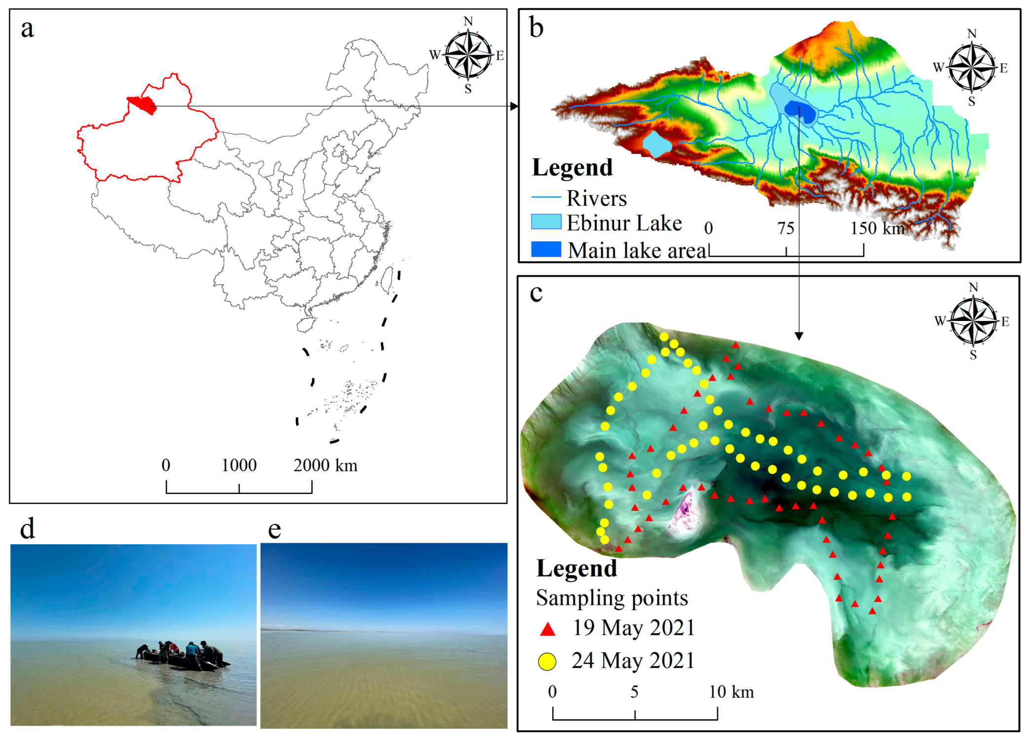
2. Overview of the Research Area

Ebinur Lake is located in Xinjiang, Northwest China (44°54′~45°08′N, 82°35′~83°10′E), and is a broken subsidence basin formed by the Himalayan orogeny (Figure 1) [34]. The lake basin is the lowest depression, with an elevation of about 190 m. Surrounded by mountains on the west, south, and north, it is located in the heart of the Eurasian continent, with little precipitation, intense evaporation, and abundant sunlight and heat. The climate is typical temperate continental, with an annual average temperature of 6.6~7.8 °C and annual precipitation of 116.0~169.2 mm. Northwest of Ebinur Lake is the famous gale mouth of Alashankou, noted as having a maximum wind speed of over 55.0 m/s for 164 days/year [35]. The lake has an average depth of 1.4 m, with a lake surface water density of about 1.079 g/cm3, pH 8.49, and a mineralization degree of 112.4 g/L [36].

3. Data Source and Processing

3.1. Water Sample Collection and Laboratory Analysis

On-site acquisition was the principal way of obtaining the basic raw data in this research, acquired on 19 and 24 May 2021, at 103 sampling points. Sampling was conducted at 11:00~16:00, Beijing time. Sentinel-2 images were taken on 19 and 24 May 2021 at 12:26 and Sentinel-3 images were taken on 19 May 2021 from 12:00 to 12:03 and 24 May from 12:10 to 12:13, with the on-site data collected at the same time as the satellite transit (±4 h), strictly following the principle of interstellar synchronization [37].
Figure 1c indicates the sampling point design at about 1.5~2 km apart. The points cover different parts of the water body. Field sampling data included GPS location, water depth, salinity, temperature, DO, and pH. Inflatable kayaks were used to move around in the lake, and 2 L water samples were collected at 0.1 to 0.3 m depth using a fine mouth polyethylene bottle. The collected water samples were kept in cold storage (<4 °C) before conducting laboratory experiments to reduce the changes in physicochemical attributes in water [38].

3.2. Images and Preprocessing

Sentinel-2, consisting of two stars, A and B, is an environmental monitoring satellite launched by the European Space Agency (ESA), capable of providing ground-based observations with high spatial and temporal resolution. It has an orbital height of 768 km and a width of 290 km, with a single-star revisit period of 10 d and a binary revisit period of 5 d. The satellite is equipped with a push-scan multispectral imager (MSI) to obtain 13 band images with spatial resolutions of 10, 20, and 60 m. Detailed band information is shown in Table 1. Obtained from the ESA platform https://scihub.copernicus.eu/dhus/#/home (accessed on 10 December 2021), the images were an atmospheric apparent reflectivity product with orthotropic and geometric precision corrections.
In this research, the Sentinel-2 images were pretreated by the Dark Spectrum Fitting (DSF) atmospheric correction algorithm, which is especially suitable for turbid water [39,40,41]. The Acolite provided by the DSF method was used to conduct atmospheric correction preprocessing https://github.com/acolite/acolite (accessed on 25 December 2021). Sentinel-2A/B data were corrected for atmosphere, processed in a batch program, exported to TIFF standard format, and then banded for synthesis. Since the Sentinel images lost three 60 m resolution bands for water vapor and SWIR-Cirrus after processing as 10 m resolution images, 11 bands were retained. They included B1-Coastal aerosol, B2-Blue, B3-Green, B4-Red, B8-NIR, B8a-Narrow NIR, B11-SWIR1, B12-SWIR2, and B5, B6, and B7 for vegetation red-edge bands. The output images were trimmed to cover the whole research area.
The Sentinel-3 satellite monitors the global ocean and land in real time. Among them, sea temperature, sea color, and sea level height data can be used to monitor climate change, ocean pollution, biological productivity [42,43,44], terrestrial forest fires, terrestrial vegetation health, and water levels of lakes and rivers [45,46,47]. The satellite has an orbital altitude of 800–830 km and a revisit period of less than 2 days. It carries a Sea-Land Surface Temperature Radiometer (SLSTR) and a Sea-Land Chromaticity Instrument (OLCI). This research mainly used the OLCI sensors, with 21 bands and a spatial resolution of 300 m, with detailed band information listed in Table 2. The data were obtained from the ESA data platform, which is an atmospheric apparent reflectivity product, using DSF atmospheric correction for Sentinel-3 OLCI [48,49]. These data were reprojected and resampled to 10 m to coincide with the image numbers of the research area in Sentinel-2 to form spatio-temporal fused data pairs to facilitate the research.

4. Methods

4.1. Spatio-Temporal Fusion Algorithm

ESTARFM, an enhanced spatio-temporal fusion algorithm proposed by Zhu et al., was used to generate fusion images of Ebinur Lake’s surface [10]. This algorithm is suitable for the lake’s constantly changing SPM, considering that the ground reflectivity may change over time. The image processing mainly required the two-stage Sentinel-2 and -3 image pairs before and after the reconstruction date and one Sentinel-3 image on the reconstruction date. The Sentinel-2 images of the day were fused through the ESTARFM model.
ESTARFM thoroughly considered the spatial heterogeneity of the Sentinel-3 (coarse spatial and high temporal resolution) image and introduced the conversion coefficient to improve the fusion simulation results. The simulated image as the central image was used to build a relatively large moving window. The average image element with similar spectral features and the central image were calculated and selected to assign the value weight. Finally, the central value was calculated. The central image value was computed by Equation (1):
L b ( x w / 2 , y w / 2 , T ) = L b ( x w / 2 , y w / 2 , T ) + i = 1 n W i × v i × ( M b ( x i , y i , T ) M b ( x i , y i , T ) )
where L b and M b represent band b of Sentinel-2 (fine space, low time resolution image) and Sentinel-3 images, respectively; w is the moving window size; ( x w / 2 , y w / 2 ) represents analog image position; T and T represent time; W i is the first image similar to analog image weight; v i represents the first and analog spectral image conversion coefficient; n is an analog which is similar to analog image number; and ( x i , y i ) represents the image position.
This study selected t 1 , t 3 of Sentinel-2/3 images as model data input, and t 2 of Sentinel-3 simulated t 2 of Sentinel-2: L b , t ( x w / 2 , y w / 2 , t 2 )   ( t = t 1 , t 2 ) . The t 2 time images simulated at t 1 , t 3 were weighted to obtain more accurate t 2 time simulation images, and the weight ε t calculation is shown in Equation (2). Equation (3) was used to calculate the simulated central image value and obtain the simulated remote sensing images with high spatio-temporal resolution.
ε t = 1 / j = 1 w i = 1 w M b ( X i , Y j , t ) j = 1 w i = 1 w M b ( X i , Y j , t 2 ) t ( 1 / j = 1 w i = 1 w M b ( x i , y j , t ) j = 1 w i = 1 w M b ( x i , y j , t 2 ) ) , t = t 1 , t 3
L b , t ( x w / 2 , y w / 2 , t 2 ) = t ε t × L b , t ( x w / 2 , y w / 2 , t ) , t = t 1 , t 3
FSDAF can predict regions of the ground type well [14]. It first classifies high-score, low-frequency images in known periods based on unsupervised classification methods. We adopted the K-means unsupervised classification method and set the classification number to four categories, a, b, c, and d, and then calculated the richness of each category in each high-frequency, low-scoring pixel using Equation (4).
f ( X , c ) = N ( X , c ) / m
where f ( X , c ) is the richness of category c in high-frequency and low-frequency pixels X in known periods, N ( X , c ) is the number of high-score and low-frequency pixels in pixel X and category c , and m is the number of high-score and low-frequency images in high-frequency and low-frequency pixel X . After we selected the high-frequency, low-score pixel with the highest richness in various categories, we found the difference between these high-frequency, low-score pixels in the known period and the prediction period and then fit the change value of the high-score, low-frequency pixel in each category by the least squares method.

4.2. Spatio-Temporal Fusion Strategy

To reconstruct the Sentinel-2 reflectance image, we needed to perform a spatio-temporal fusion operation based on the Sentinel-3 reflectance image. Among them, blue, green, red, and NIR are important visible light bands to monitor lake SPM [49]. As shown in Figure 2, they are also bands within the common spectral range of Sentinel-2 and Sentinel-3, with similar central wavelengths, and are an important remote sensing data basis for establishing spatio-temporal fusion models [14].
In this research, the model was tested by using two image data pairs to further reduce information loss in the fusion results with different input image pairs that were used. There are a total of six fusion results for the (a) and (b) fusion strategies in Figure 3.
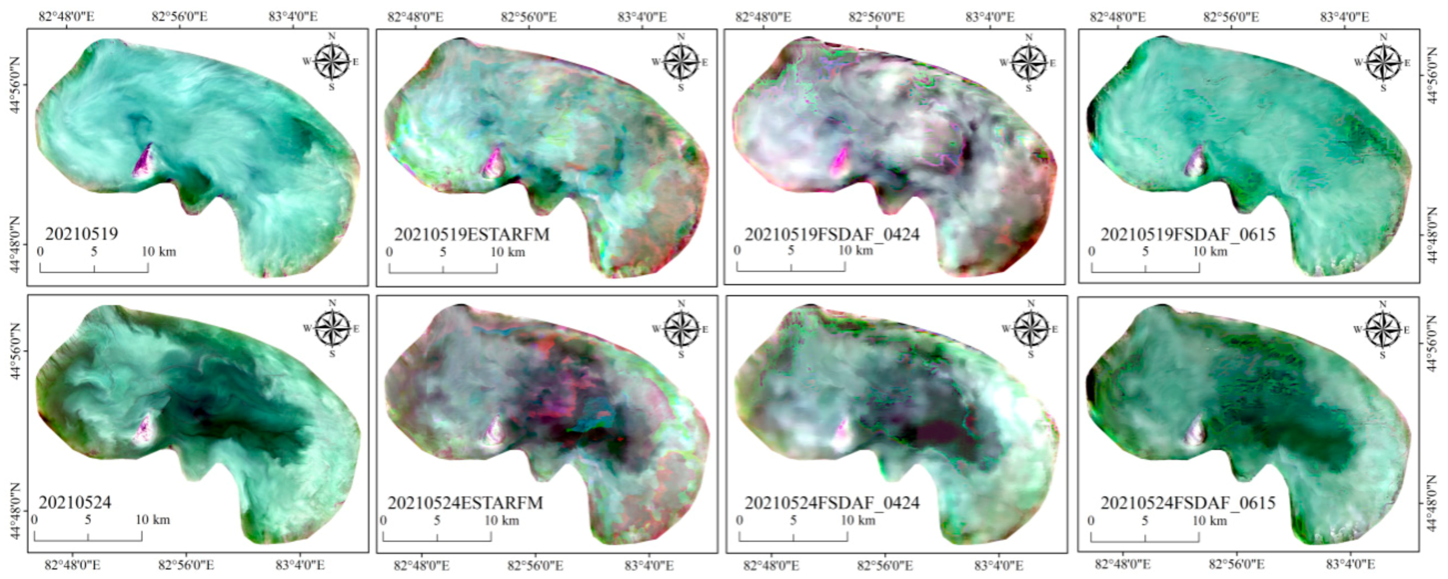
  • Fusion Strategies: The images (pixel 10 m) of Ebinur Lake on 19 and 24 May 2021 were used as reconstruction targets, and data pairs from different time points were used as inputs for ESTARFM and FSDAF models to reconstruct the optimal reflectance images. Firstly, Sentinel-2 and -3 images presented on 15 June and 24 April 2021 served as input image pairs for the ESTARFM model. According to the Sentinel-3 image on 19 and 24 May 2021, the ESTARFM fusion remote sensing image with a spatial resolution of 10 m was predicted. Secondly, the Sentinel-2 and -3 image pairs from 15 June and 24 April 2021 were used as input to the FSDAF model. The Sentinel-3 images on 19 and 24 May 2021 were used to predict FSDAF fusion images on the same date. Thirdly, the fused ESTARFM, FSDAF0424, and FSDAF0516 images were analyzed, validated, and compared with the original Sentinel-2 reference images on both sampling days (Figure 4), The small color differences in the fused images are mainly caused by errors in the fused bands. Finally, the SPM concentration inversion was performed on the fused images.
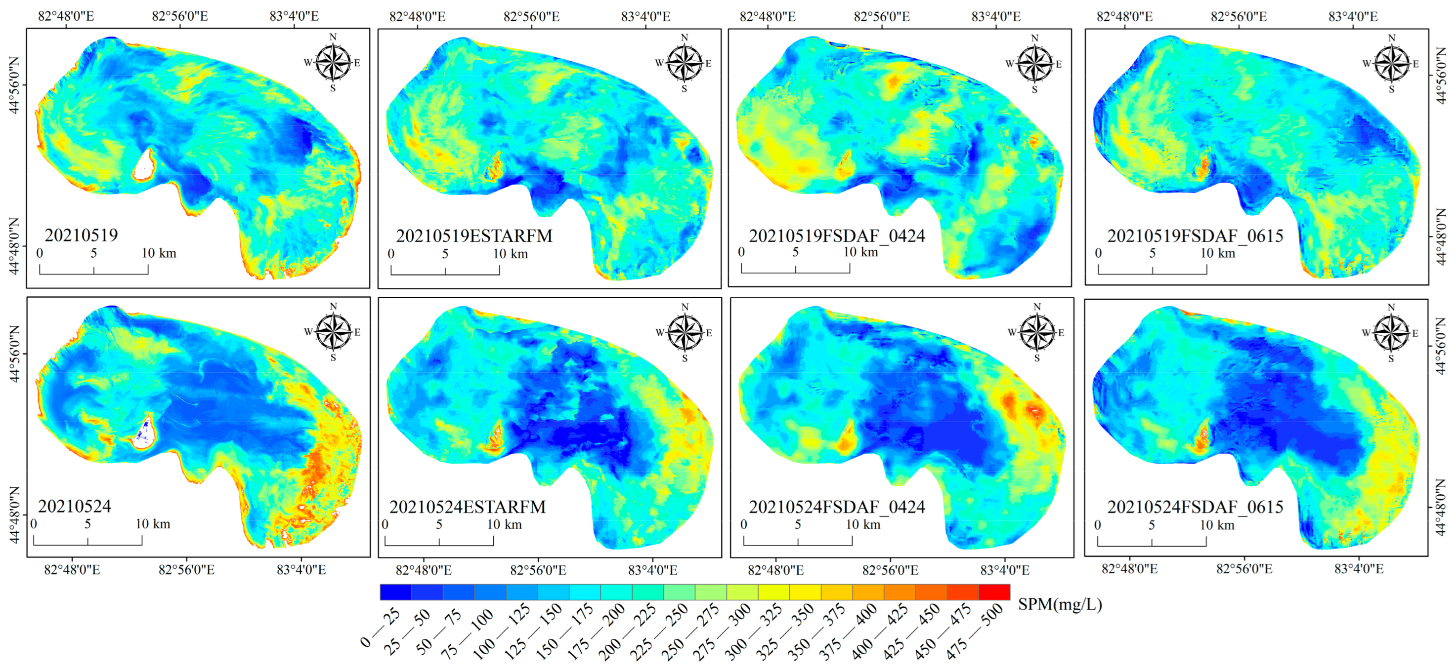
  • Fusion Strategies: The Ebinur Lake SPM concentration map on 19 and 24 May 2021 was used as the reconstruction target. The Sentinel-2 and -3 SPM concentration inversion maps on 15 June and 24 April 2021 were used as the input image pairs for the ESTARFM model. ESTARFM fused SPM maps with a spatial resolution of 10 m that were predicted based on the Sentinel-3 images of 19 and 24 May 2021.

4.3. Spatio-Temporal Fusion Images Evaluation Indicators

To quantitatively research the quality of spatial and reference image quality, the Pearson correlation coefficient (R) was selected [50], along with normalized root mean square error (RMSE), peak signal-to-noise ratio (PSNR), and structural similarity (SSIM) to evaluate image quality [51]. The reference image I size was m × n and the spatio-temporal fusion image was F; I ( i , j ) was the reference image value and F ( i , j ) was the spatio-temporal fusion image value.
R evaluated the degree of consistency between spatio-temporal fusion images and reference images using Equation (5):
R = i = 1 m j = 1 n ( I ( i , j ) I ¯ ) ( F ( i , j ) F ¯ ) i = 1 m j = 1 n ( I ( i , j ) I ¯ ) 2 i = 1 m j = 1 n ( F ( i , j ) F ¯ 2 )
RMSE refers to the square root of the deviation between the spatio-temporal fusion image and the reference image, calculated by Equation (6):
RMSE = i = 1 m j = 1 n ( I ( i , j ) F ( i , j ) ) 2 m n
PSNR was used to evaluate the amount of fusion image information. A large value represents less image information loss. The mean square error M S E was computed by Equation (7) and PSNR by Equation (8):
M S E = 1 m n i = 0 m 1 j = 0 n 1 [ I ( i , j ) F ( i , j ) ] 2
PSNR = 10 log 10 M A X ( i , j ) 2 M S E
where M A X ( i , j ) is the maximum image value of the image.
SSIM evaluated the structural similarity between spatio-temporal fusion images and reference images, calculated by Equation (9):
SSIM = ( 2 u I u F + C 1 ) ( 2 σ I F + C 2 ) ( u I 2 + u F 2 + C 1 ) ( σ I 2 + σ F 2 + C 2 ) )
where u I and u F represent the mean, σ I and σ F represent the variance between the reference image and the fused image, and σ I F represents the covariance between the two images. C 1 and C 2 are two constants close to 0 used to stabilize the results. An SSIM value close to 1 indicates high structural similarity between the two images.

4.4. SPM Evaluation Indicators

The coefficient of determination (R2), root mean square error (RMSE), mean absolute percentage error (MAPE), and deviation (bias) test whether the predicted and measured values are consistent. R2 describes the degree to which the independent variable (remote sensing reflectance) explains the dependent variable (SPM concentration) [52,53]. It is usually used for auxiliary evaluation of model performance. A higher R2 value should not be excessively pursued in building this high-precision model because it is prone to overfitting the modeling data. Moreover, accuracy may drop if the independent validation data are used to verify the overfitted model. Therefore, a larger R2 does not mean that the model is invariably applicable. In balance, multiple indicators are needed to evaluate the model’s reliability.
R2 evaluated the degree of consistency between predictions and true values using Equation (10):
R 2 = 1 i = 1 n ( y i y ^ ) 2 i = 1 n ( y i y ¯ ) 2
RMSE is the square root of the ratio of the forecast and the image matrix, computed by Equation (11):
RMSE = i = 1 n ( y i y ^ ) 2 n
MAPE represents the percentage of the absolute value of the predicted value, calculated by Equation (12):
M A P E = 1 n i = 1 i n y i y ^ i y i × 100 %
Bias represents the deviation from the predicted value and the true value, computed by Equation (13):
B i a s = 1 n i = 1 n y i y ^ i

5. Results and Analysis

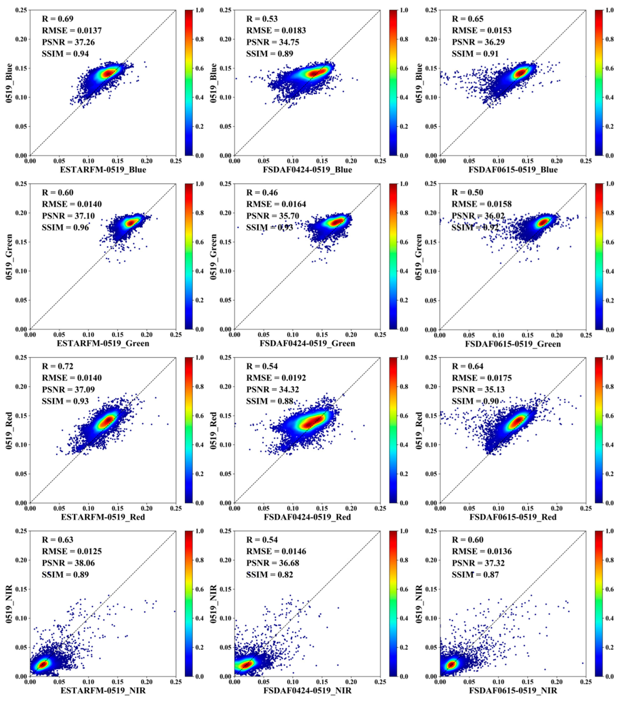
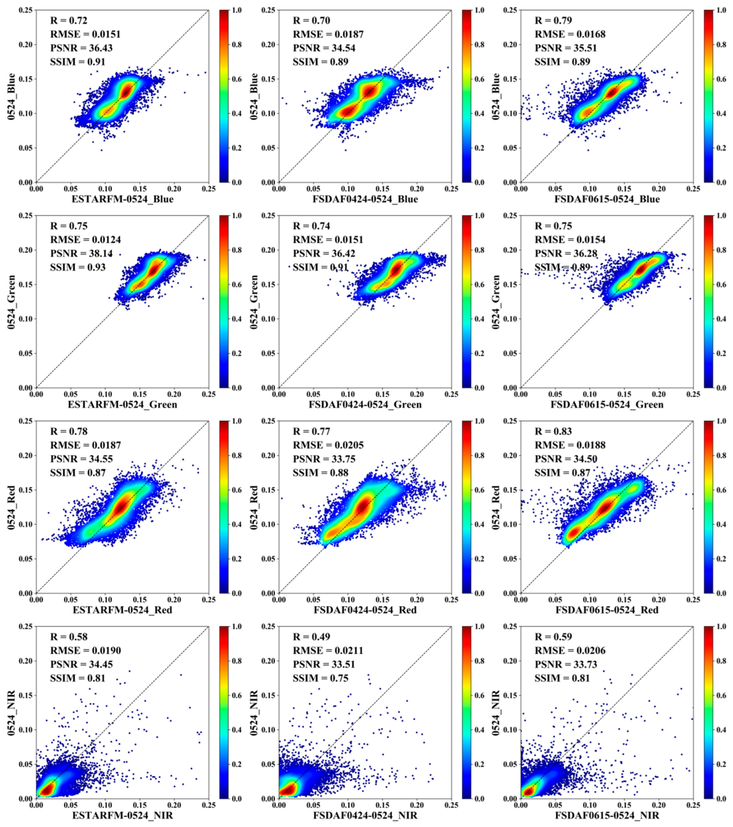
5.1. Spatio-Temporal Fusion Reflectance Image Reconstruction and Evaluation

Figure 4 compares the ESTARFM and FSDAF fusion images with the reference images. By using blue, green, and red true color band channels to display the lake images, the visual discrimination of the spatio-temporal fusion model can better realize the generation of predicted date images.
Four evaluation indicators were applied to assess the fusion images to further quantitatively evaluate the image quality and retention of spectral information (Figure 5). The overall image quality of the ESTARFM fusion image on 19 May 2021 was better than that of the FSDAF. The evaluation indicators R, RMSE, PSNR, and SSIM in the blue band verified that the ESTARFM fusion image had the best quality; the FSDAF0615 ranked second, and the FSDAF0424 was the last. Using the green band indicators, the ESTARFM fusion image remained the best, and the FSDAF0615 accuracy was slightly higher than FSDAF0424. For the red band indicators, the ESTARFM fusion image also had the best quality (R was 0.72, RMSE was 0.0140, PSNR was 37.09, and SSIM was 0.93). Finally, in the NIR band, the accuracy of the FSDAF0424 fusion image was relatively poor, whereas the accuracy difference between FSDAF0615 and ESTARFM was small.
The concentration of the plotted points in a small core area along the 1:1 line and limited dispersion away from the core to the periphery signify a good match between the fusion and reference images (Figure 5). In the blue band, the ESTARFM model with the smallest point spread and the most prominent concentration indicated the best distribution and effects of the three. The FSDAF0424 model showed relatively more point scattering in the core and peripheral areas. The FSDAF0615 model demonstrated a concentration in the core area, with large prediction errors in the low-value area. In the green band, the FSDAF0424 model had quite bundled points, but the FSDAF0615 model displayed more errors in the low-value area. The red band had the best effects compared with other bands, with more points clustering along and adjacent to the 1:1 line. The ESTARFM model registered the best performance, and the FSDAF0424 had a relatively more scattered distribution in the core and peripheral areas. Although the FSDAF0615 model demonstrated a concentration in the core area, it had more fusion errors in the low-value area. For the NIR band, the three graphs showed heavy crowding in the lowest-value part adjoining the origin. However, some points were dispersed to the medium- and high-value areas. Such patterns indicated relatively large discrepancies between the fusion and reference images.
Using the 24 May 2021 images, we further investigated the accuracy of fusion images with the same evaluation indicators (Figure 6). The overall image quality of ESTARFM was better than FSDAF. Among these indicators, the results of R evaluation conflict with those jointly evaluated by RMSE, PSNR, and SSIM. In other words, the accuracy of RMSE, PSNR, and SSIM of ESTARFM model is higher than that of FSDAF0615, while R is on the contrary, reflecting that R cannot evaluate image quality to a certain extent. Therefore, we applied three indicators to evaluate the blue band; the ESTARFM fusion image quality was the best, followed by FSDAF0615 and then FSDAF0424. However, in the green band, the ESTARFM fusion image had the best quality effect, whereas FSDAF0615 and FSDAF0424 were of poor quality. In the red band, the ESTARFM fusion image had the best quality effect. In the NIR band, FSDAF0424 and FSDAF0615 fusion images had relatively poor accuracy, and ESTARFM had relatively good accuracy.
From the scatter distribution analysis in Figure 6, we found that in the blue band, the ESTARFM model denoted pronounced point concentration and suitable accuracy and that the FSDAF0424 model had scattered to the high-value area versus the FSDAF0615 model’s scattering to the low-value area. In the green band, the prediction errors of FSDAF0424 also appeared in the high-value area, and the FSDAF0615 had prediction errors mainly in the middle-value area. In the red band, the three fusion images demonstrated the best distribution, with a concentration near the 1:1 line, compared with other bands. The ESTARFM model showed the best effect. For the NIR band, the results were similar to 19 May 2021. Most points were bundled in the lowest-value area around the graph origin. A notable number of points dispersed to the middle and high-value areas, signifying considerable errors in image prediction.

5.2. Construction of the SPM Inversion Models for Sentinel-2 and Sentinel-3

The light absorption and scattering properties of various substances in the lake water determine the spectral reflection characteristics of the water body [54]. Changes in the composition and concentration of SPM in Ebinur Lake trigger corresponding changes in spectral reflection characteristics. From Figure 7, the SPM reflectance information of Sentinel-2 and Sentinel-3 is higher in the red, green, and blue bands and lower in the NIR band, and the reflectance information of SPM sampling points is best separated in the red band. These results provided a basis to establish the Sentinel-2 and Sentinel-3 regression models.
Section 5.1 shows that the fusion red band had the highest accuracy. Therefore, the red band was chosen for the inversion of SPM in this research. In the SPSS software, the red band was used as the independent input variable in the modeling, and the measured SPM concentration was regression-analyzed as the dependent variable. The 73 (70%) random samples of the 103 matched sample pairs were used to build the regression model. The remaining 30 (30%) sample pairs were used to test model accuracy. Mathematical models were built for the red bands, with the regression coefficients solved and R2 determined (Table 3).
The sample distribution in the scatter plot of the red band (Figure 8) showed that the SPM concentration fit the reflectance well, but some samples were dispersed in the high-value region. Table 3 indicates that the fitting effects of the models were suitable. The R2 of the Sentinel-2 exponential model was the highest at 0.63, and the linear model had the lowest R2 at 0.47. The R2 of the Sentinel-3 exponential model was the highest at 0.73, and the linear model had the lowest R2 at 0.65.
To quantify the accuracy of these models, the common evaluation indicators RMSE, MAPE, and bias were applied for comparison. Figure 9 indicates that the minimum RMSE of the red band model based on Sentinel-2 was 35.47 mg/L, and the minimum MAPE was 15.30%. The minimum bias based on the polynomial model was −1.42 mg/L.
It can be seen from Figure 10 that the minimum RMSE and the minimum MAPE of the red band polynomial model based on Sentinel-3 were 43.59 mg/L and 16.05%, respectively. The minimum bias based on the red band linear model was −19.33 mg/L.

5.3. SPM Images Reconstruction Strategy

5.3.1. Estimation of SPM Using the Spatio-Temporal Fusion Reflectance Image

The results were compared with the red band SPM concentration estimates of the reference image (Figure 11). The three fusion images recorded on both sampling days could reflect the general trend of the SPM concentration distribution.
The accuracy estimation results of the SPM concentrations of different fusion models on both sampling days were compared (Figure 12). The overall evaluation indicators showed that the fusion image estimate on 24 May 2021 was better than that on 19 May 2021. Among the fusion models, the SPM concentration accuracy of the ESTARFM image inversion was the best on 19 May 2021. The evaluation indicators on 24 May 2021 showed that the ESTARFM image inversion had lower accuracy than FSDAF0615, but the RMSE difference was small.
The ESTARFM fusion image estimate yielded the best results among the three scatter density graphs of the SPM concentration for 19 May 2021. The FSDAF0424 and FSDAF0615 models showed different distribution patterns. For the 24 May 2021 graph, the ESTARFM fusion image estimates were the best, with a high concentration in the core area and less dispersion compared with the FDSAF0615 and FSDAF0424 models.
In sum, the fusion image quality of the ESTARFM model satisfied various evaluation indicators and had adequate stability. The FSDAF model showed some uncertainty, with accuracy sometimes depending on the input images. Therefore, a reliable ESTARFM model was adopted in the subsequent analysis.

5.3.2. Spatio-Temporal Fusion SPM

The raw images from Sentinel-2 and -3 were used to invert SPM concentrations (Section 5.1 and Section 5.2). The SPM concentration inversion maps on 24 April and 15 June 2021 were used as the data pairs. The SPM concentration inversion maps on 19 May and 24 May 2021 were used as data sources. The estimated results were compared with the reference image results (Figure 13). The fusion images on both sampling days could better reflect the general SPM concentration trend. Analysis of different fusion strategies indicated that the SPM spatio-temporal fusion accuracy was higher (Figure 14). The image performance based on the evaluation indicators alone was sufficient. Analysis of different data sources signified that the fusion SPM estimate on 24 May 2021 was better than that on 19 May 2021.
Figure 14 further shows that the SPM inversion accuracy was higher before fusion. The ESTARFM model and the after-fusion inversion strategy were adopted to generate spatio-temporal fusion images to complement the missing high-resolution SPM distribution maps.

6. Discussion

6.1. Spatio-Temporal Fusion Algorithm

Spatio-temporal fusion models have been widely used to research land use cover, vegetation, soils, water bodies, and other spectral reflectance imagery [8]. Han et al. briefly compared the accuracy of four spatio-temporal fusion algorithms (STARFM, ESTARFM, FSDAF, and FITFC) with R ranging from 0.621 to 0.907 and RMSE ranging from 0.019 to 0.08 using MODIS (500 m) Landsat-8 and Sentinel-2 as input data pairs, and concluded that their fused reflectance image accuracies all met their research requirements [55]. In this research, a comparison of two time points was used as a predictor to test the stability of the model. The ESTARFM model had R ranging from 0.58 to 0.78 and RMSE from 0.019 to 0.0124, while the FSDAF model had R ranging from 0.46 to 0.83 and RMSE from 0.0211 to 0.0136. As a result, it can be seen that the ESTARFM model in this research had a smaller and more stable margin of error. A comparative analysis of ESTARFM and FSDAF models was carried out to apply the spatio-temporal fusion model to lake SPM research, further demonstrating the feasibility of applying the spatio-temporal fusion model to the inversion of SPM in water bodies.

6.2. Accuracy of SPM Models

In this research, a more convenient and fast regression model was used for SPM inversion modeling, providing that sufficient sample points were collected from the lake [56,57,58]. Firstly, the inverse model has suitable interpretability. Secondly, the focus of this research was to conduct a spatio-temporal fusion strategy study, and the use of a convenient and fast modeling approach helped to reduce the transmission of errors and the mitigation of uncertainty in modeling. When modeling with the four regression models, it was found through Figure 6 that the SPM spectral information in the red band was better separated and therefore modeled with red. However, after the four models were built, their validation revealed that when the models were applied to Sentinel-2 (Figure 8), the power and exponential models, although better modeled with R2 values of 0.62 and 0.63, respectively, had larger bias for validation, while the accuracy of the polynomial model was slightly better than the linear model, and both could be inverted for SPM concentration. When the model was applied to Sentinel-3 (Figure 9), it was found that the power and exponential models were better modeled, with R2 values of 0.72 and 0.73, respectively, again with larger bias and RMSE at validation, while the linear model had better bias metrics than the polynomial model when the other metrics were not too different from the polynomial model. In summary, to avoid systematic error transfer due to inconsistencies in the modeling model formulations, given the small differences in model accuracy, Sentinel-2 and Sentinel-3 both use a linear model with a simpler model structure and the highest accuracy requirements for the later spatio-temporal fusion strategy.

6.3. Spatio-Temporal Fusion Strategy

The spatio-temporal fusion algorithm is primarily based on the fusion of remote sensing images and then the inversion of the target SPM. In this way, during the fusion of the target SPM, the target SPM information is more or less lost due to differences in the quality and timing of the input image pairs and the calculation methods of different spatio-temporal fusion models.
The accuracy validation evaluation of Figure 12 and Figure 14 reveals that both strategies a and b from Figure 3 can have suitable fusion accuracy and that the closer the time is to the fusion target, the better the accuracy of the fused image, with R ranging from 0.55 to 0.84, RMSE from 52.30 to 34.70 mg/L, PSNR from 25.97 to 29.20 dB, and SSIM from 0.65 to 0.77 for strategy a, while strategy b has R ranging from 0.72 to 0.83, RMSE ranging from 35.10 to 32.50 mg/L, PSNR from 29.09 to 29.76 dB, and SSIM from 0.75 to 0.79. It can be seen that the fusion results for strategy a with high and low accuracy are generated by the FSDAF model, indicating that there is high instability in the FSDAF model, which is detrimental to our future extension applications. At the same time, the accuracy advantage of the ESTARFM model fusion results for strategy b over a is also all-encompassing, which better informs future similar studies and further clarifies the specific impact of the different spatio-temporal fusion strategies on the results. Another important reason for the greater stability of ESTARFM may also be that the input data pairs are two pairs, whereas FSDAF has only one pair of input data pairs, which also provides an idea for future research. Thus, we will explore the effect of models with two input pairs or one input pair on the results in the next step. However, for this research, the use of different fusion strategies plays a decisive role in the reconstruction of SPM images, and fusing target water quality images has an all-around better accuracy performance than fusing reflection images.

7. Conclusions

Based on the measured SPM concentration data and Sentinel-2 and -3 images, the optimal SPM inversion model and data reconstruction strategy with adequate capabilities and suitability were identified. From the results, we drew the following conclusions:
  • The ESTARFM fusion of blue, green, red, and NIR bands was the best, among which the red band had the highest accuracy.
  • The red band was determined to be the best choice for regression modeling based on an accurate assessment of the measurements and model stability analysis.
  • The fused SPM concentration map proved to be better and more stable.
In future research, we could use more accurate physical models or semi-physical models to carry out the research. In the meantime, we are prepared to adopt the incorporation or improvement of more spatio-temporal fusion algorithms for comparative studies to further enhance the applicability and scalability of our research.

Author Contributions

Conceptualization, P.D.; methodology, P.D.; software, P.D.; validation, P.D.; formal analysis, F.Z.; investigation, Y.C.; resources, F.Z. and Y.C.; data curation, P.D., Y.C., C.L., W.W. and Z.W.; writing—original draft preparation, P.D.; writing—review and editing, P.D., C.-Y.J., M.L.T. and J.S.; visualization, P.D., M.L.T. and J.S.; supervision, F.Z.; project administration, F.Z.; funding acquisition, F.Z. All authors have read and agreed to the published version of the manuscript.

Funding

This research was funded by the National Natural Science Foundation of China (Grant Number 42261006), the State Key Laboratory of Lake Science and Environment (Grant Number 2022SKL007, and the Tianshan Talent Project (Phase III) of the Xinjiang Uygur Autonomous Region.

Data Availability Statement

The data presented in this study are available on request from the corresponding author. The data are not publicly available due to confidentiality.

Acknowledgments

We appreciate the helpful comments offered by the anonymous reviewers and editors to improve our manuscript.

Conflicts of Interest

The authors declare no conflict of interest.

References

  1. Liu, C.; Zhang, F.; Wang, X.; Chan, N.W.; Rahman, H.A.; Yang, S.; Tan, M.L. Assessing the factors influencing water quality using environment water quality index and partial least squares structural equation model in the Ebinur Lake Watershed, Xinjiang, China. Environ. Sci. Pollut. Res. 2022, 29, 29033–29048. [Google Scholar] [CrossRef]
  2. Liu, D.; Abuduwaili, J.; Lei, J.; Wu, G.; Gui, D. Wind erosion of saline playa sediments and its ecological effects in Ebinur Lake, Xinjiang, China. Environ. Earth Sci. 2011, 63, 241–250. [Google Scholar] [CrossRef]
  3. Sagan, V.; Peterson, K.T.; Maimaitijiang, M.; Sidike, P.; Sloan, J.; Greeling, B.A.; Maalouf, S.; Adams, C. Monitoring inland water quality using remote sensing: Potential and limitations of spectral indices, bio-optical simulations, machine learning, and cloud computing. Earth-Sci. Rev. 2020, 205, 103187. [Google Scholar] [CrossRef]
  4. Liu, C.; Duan, P.; Zhang, F.; Jim, C.Y.; Tan, M.L.; Chan, N.W. Feasibility of the spatiotemporal fusion model in monitoring Ebinur Lake’s suspended particulate matter under the missing-data scenario. Remote Sens. 2021, 13, 3952. [Google Scholar] [CrossRef]
  5. Li, J.; Li, Y.; He, L.; Chen, J.; Plaza, A. A new sensor bias-driven spatio-temporal fusion model based on convolutional neural networks. Sci. China Inf. Sci. 2020, 63, 1–17. [Google Scholar] [CrossRef]
  6. Shevyrnogov, A.; Trefois, P.; Vysotskaya, G. Multi-satellite data merge to combine NOAA AVHRR efficiency with Landsat-6 MSS spatial resolution to study vegetation dynamics. Adv. Space Res. 2000, 26, 1131–1133. [Google Scholar] [CrossRef]
  7. Malenovsky, Z.; Bartholomeus, H.M.; Acerbi-Junior, F.W.; Schopfer, J.T.; Painter, T.H.; Epema, G.F.; Bregt, A.K. Scaling dimensions in spectroscopy of soil and vegetation. Int. J. Appl. Earth Obs. Geoinf. 2007, 9, 137–164. [Google Scholar] [CrossRef]
  8. Sun, L.; Gao, F.; Xie, D.H.; Anderson, M.; Chen, R.; Yang, Y.; Yang, Y.; Chen, Z. Reconstructing daily 30m NDVI over complex agricultural landscapes using a crop reference curve approach. Remote Sens. Environ. 2020, 253, 112156. [Google Scholar] [CrossRef]
  9. Gao, F.; Masek, J.; Schwaller, M.; Hall, F. On the blending of the Landsat and MODIS surface reflectance: Predicting daily Landsat surface reflectance. IEEE Trans. Geosci. Remote Sens. 2006, 44, 2207–2218. [Google Scholar]
  10. Zhu, X.; Chen, J.; Gao, F.; Chen, X.; Masek, J.G. An enhanced spatial and temporal adaptive reflectance fusion model for complex heterogeneous regions. Remote Sens. Environ. 2010, 114, 2610–2623. [Google Scholar] [CrossRef]
  11. Cheng, Q.; Liu, H.; Shen, H.; Wu, P.; Zhang, L. A spatial and temporal nonlocal filter-based data fusion method. IEEE Trans. Geosci. Remote Sens. 2017, 55, 4476–4488. [Google Scholar] [CrossRef] [Green Version]
  12. Wu, M.; Huang, W.; Niu, Z.; Wang, C. Generating daily synthetic Landsat imagery by combining Landsat and MODIS data. Sensors 2015, 15, 24002–24025. [Google Scholar] [CrossRef] [PubMed]
  13. Xie, D.; Zhang, J.; Zhu, X.; Pan, Y.; Liu, H.; Yuan, Z.; Yun, Y. An improved STARFM with help of an unmixing-based method to generate high spatial and temporal resolution remote sensing data in complex heterogeneous regions. Sensors 2016, 16, 207. [Google Scholar] [CrossRef] [PubMed]
  14. Zhu, X.; Helmer, E.H.; Gao, F.; Liu, D.; Chen, J.; Lefsky, M.A. A flexible spatiotemporal method for fusing satellite images with different resolutions. Remote Sens. Environ. 2016, 172, 165–177. [Google Scholar] [CrossRef]
  15. Wang, L.; Wang, X.; Wang, Q.; Atkinson, P.M. Investigating the influence of registration errors on the patch-based spatio-temporal fusion method. IEEE J. Sel. Top. Appl. Earth Obs. Remote Sens. 2020, 13, 6291–6307. [Google Scholar] [CrossRef]
  16. Huang, B.; Song, H. Spatiotemporal reflectance fusion via sparse representation. IEEE Trans. Geosci. Remote Sens. 2012, 50, 3707–3716. [Google Scholar] [CrossRef]
  17. Li, W.; Zhang, X.; Peng, Y.; Dong, M. Spatiotemporal fusion of remote sensing images using a convolutional neural network with attention and multiscale mechanisms. Int. J. Remote Sens. 2021, 42, 1973–1993. [Google Scholar] [CrossRef]
  18. Song, H.; Liu, Q.; Wang, G.; Hang, R.; Huang, B. Spatiotemporal satellite image fusion using deep convolutional neural networks. IEEE J. Sel. Top. Appl. Earth Obs. Remote Sens. 2018, 11, 821–829. [Google Scholar] [CrossRef]
  19. Tan, Z.; Cao, Z.; Shen, M.; Chen, J.; Song, Q.; Duan, H. Remote estimation of water clarity and suspended particulate matter in qinghai lake from 2001 to 2020 using MODIS images. Remote Sens. 2022, 14, 3094. [Google Scholar] [CrossRef]
  20. Du, Y.; Song, K.; Liu, G.; Wen, Z.; Fang, C.; Shang, Y.; Zhao, F.; Wang, Q.; Du, J.; Zhang, B. Quantifying total suspended matter (TSM) in waters using Landsat images during 1984–2018 across the Songnen Plain, Northeast China. J. Environ. Manag. 2020, 262, 110334. [Google Scholar] [CrossRef]
  21. Ford, R.T.; Vodacek, A. Determining improvements in Landsat spectral sampling for inland water quality monitoring. Sci. Remote Sens. 2020, 1, 100005. [Google Scholar] [CrossRef]
  22. Liang, Z.; Zou, R.; Chen, X.; Ren, T.; Su, H.; Liu, Y. Simulate the forecast capacity of a complicated water quality model using the long short-term memory approach. J. Hydrol. 2020, 581, 124432. [Google Scholar] [CrossRef]
  23. Flink, P.; Lindell, L.T.; Östlund, C. Statistical analysis of hyperspectral data from two Swedish lakes. Sci. Total Environ. 2001, 268, 155–169. [Google Scholar] [CrossRef]
  24. Rotta, L.; Alcântara, E.; Park, E.; Bernardo, N.; Watanabe, F. A single semi-analytical algorithm to retrieve chlorophyll-a concentration in oligo-to-hypereutrophic waters of a tropical reservoir cascade. Ecol. Indic. 2021, 120, 106913. [Google Scholar] [CrossRef]
  25. Nechad, B.; Ruddick, K.G.; Park, Y. Calibration and validation of a generic multisensor algorithm for mapping of total suspended matter in turbid waters. Remote Sens. Environ. 2010, 114, 854–866. [Google Scholar] [CrossRef]
  26. Alcântara, E.; Curtarelli, M.; Ogashawara, I.; Rosan, T.; Kampel, M.; Stech, J. Developing QAA-based retrieval model of total suspended matter concentration in Itumbiara reservoir. In Proceedings of the Brazil//2015 IEEE International Geoscience and Remote Sensing Symposium (IGARSS), Milan, Italy, 26–31 July 2015; pp. 711–714. [Google Scholar]
  27. Sun, D.; Qiu, Z.; Hu, C.; Wang, S.; Wang, L.; Zheng, L.; Peng, T.; He, Y. A hybrid method to estimate suspended particle sizes from satellite measurements over Bohai Sea and Yellow Sea. J. Geophys. Res. Ocean. 2016, 121, 6742–6761. [Google Scholar] [CrossRef]
  28. Lei, S.; Xu, J.; Li, Y.; Li, L.; Lyu, H.; Liu, G.; Chen, Y.; Lu, C.; Tian, C.; Jiao, W. A semi-analytical algorithm for deriving the particle size distribution slope of turbid inland water based on OLCI data: A case study in Lake Hongze. Environ. Pollut. 2021, 270, 116288. [Google Scholar] [CrossRef]
  29. Salama, M.S.; Verhoef, W. Two-stream remote sensing model for water quality mapping: 2SeaColor. Remote Sens. Environ. 2015, 157, 111–122. [Google Scholar] [CrossRef]
  30. Liu, D.; Duan, H.; Yu, S.; Shen, M.; Xue, K. Human-induced eutrophication dominates the bio-optical compositions of suspended particles in shallow lakes: Implications for remote sensing. Sci. Total Environ. 2019, 667, 112–123. [Google Scholar] [CrossRef]
  31. Kishino, M.; Tanaka, A.; Ishizaka, J. Retrieval of chlorophyll a, suspended solids, and colored dissolved organic matter in Tokyo Bay using ASTER data. Remote Sens. Environ. 2005, 99, 66–74. [Google Scholar] [CrossRef]
  32. Wei, J.W.; Wang, M.H.; Jiang, L.D.; Yu, X.; Mikelsons, K.; Shen, F. Global Estimation of Suspended Particulate Matter From Satellite Ocean Color Imagery. J. Geophys. Res. Ocean. 2021, 126, e2021JC017303. [Google Scholar] [CrossRef] [PubMed]
  33. Liu, X.; Wang, M. Global daily gap-free ocean color products from multi-satellite measurements. Int. J. Appl. Earth Obs. Geoinf. 2022, 108, 102714. [Google Scholar] [CrossRef]
  34. Zhu, S.D.; Zhang, F.; Zhang, Z.Y.; Kung, H.; Yushanjiang, A. Hydrogen and oxygen isotope composition and water quality evaluation for different water bodies in the Ebinur Lake Watershed, Northwestern China. Water 2019, 11, 2067. [Google Scholar] [CrossRef]
  35. Wang, L.; Li, Z.; Wang, F.; Li, H.; Wang, P. Glacier changes from 1964 to 2004 in the Jinghe River basin, Tien Shan. Cold Reg. Sci. Technol. 2014, 102, 78–83. [Google Scholar] [CrossRef]
  36. Liu, C.J.; Zhang, F.; Johnson, V.C.; Duan, P.; Kung, H.T. Spatio-temporal variation of oasis landscape pattern in arid area: Human or natural driving? Ecol. Indic. 2021, 125, 107495–107509. [Google Scholar] [CrossRef]
  37. Catherine, K.; Aline, D.M.V.; Nick, W.; Luke, L.; Henrique, O.S.; Milton, K.; Jeffrey, R.; Philipp, S.; John, C.; Rob, S.; et al. Performance of Landsat-8 and Sentinel-2 surface reflectance products for river remote sensing retrievals of chlorophyll-a and turbidity. Remote Sens. Environ. 2019, 224, 104–118. [Google Scholar]
  38. Wen, Z.; Wang, Q.; Liu, G.; Jacinthe, P.A.; Wang, X.; Lyu, L.; Tao, H.; Ma, Y.; Duan, H.; Shang, Y.; et al. Remote sensing of total suspended matter concentration in lakes across China using Landsat images and Google Earth Engine. ISPRS J. Photogramm. Remote Sens. 2022, 187, 61–78. [Google Scholar] [CrossRef]
  39. Vanhellemont, Q.; Ruddick, K. Atmospheric correction of Sentinel-3 OLCI data for mapping of suspended particulate matter and chlorophyll-a concentration in Belgian turbid coastal waters. Remote Sens. Environ. 2021, 256, 112284. [Google Scholar] [CrossRef]
  40. Tavares, M.H.; Lins, R.C.; Harmel, T.; Fragoso, C.R., Jr.; Martínez, J.M.; Motta-Marques, D. Atmospheric and sunglint correction for retrieving chlorophyll-a in a productive tropical estuarine-lagoon system using Sentinel-2 MSI imagery. ISPRS J. Photogramm. Remote Sens. 2021, 174, 215–236. [Google Scholar] [CrossRef]
  41. Vanhellemont, Q. Adaptation of the dark spectrum fitting atmospheric correction for aquatic applications of the Landsat and Sentinel-2 archives. Remote Sens. Environ. 2019, 225, 175–192. [Google Scholar] [CrossRef]
  42. Rieu, P.; Moreau, T.; Cadier, E.; Raynal, M.; Clerc, S.; Donlon, C.; Borde, F.; Boy, F.; Maraldi, C. Exploiting the Sentinel-3 tandem phase dataset and azimuth oversampling to better characterize the sensitivity of SAR altimeter sea surface height to long ocean waves. Adv. Space Res. 2021, 67, 253–265. [Google Scholar] [CrossRef]
  43. Xu, W.; Wooster, M.J.; Polehampton, E.; Yemelyanova, R.; Zhang, T. Sentinel-3 active fire detection and FRP product performance-Impact of scan angle and SLSTR middle infrared channel selection. Remote Sens. Environ. 2021, 261, 112460. [Google Scholar] [CrossRef]
  44. Xu, J.; Zhao, Y.; Lyu, H.; Liu, H.; Dong, X.; Li, Y.; Cao, K.; Xu, J.; Li, Y.; Wang, H.; et al. A semianalytical algorithm for estimating particulate composition in inland waters based on Sentinel-3 OLCI images. J. Hydrol. 2022, 608, 127617. [Google Scholar] [CrossRef]
  45. Zarei, A.; Shah-Hosseini, R.; Ranjbar, S.; Hasanlou, M. Validation of non-linear split window algorithm for land surface temperature estimation using Sentinel-3 satellite imagery: Case study; Tehran Province, Iran. Adv. Space Res. 2021, 67, 3979–3993. [Google Scholar] [CrossRef]
  46. Gou, J.; Tourian, M.J. Riwi. SAR-SWH: A data-driven method for estimating significant wave height using Sentinel-3 SAR altimetry. Adv. Space Res. 2022, 69, 2061–2080. [Google Scholar] [CrossRef]
  47. Odebiri, O.; Mutanga, O.; Odindi, J. Deep learning-based national scale soil organic carbon mapping with Sentinel-3 data. Geoderma 2022, 411, 115695. [Google Scholar] [CrossRef]
  48. Pahlevan, N.; Smith, B.; Schalles, J.; Binding, C.; Cao, Z.; Ma, R.; Alikas, K.; Kangro, K.; Gurlin, D.; Hà, N.; et al. Seamless retrievals of chlorophyll-a from Sentinel-2 (MSI) and Sentinel-3 (OLCI) in inland and coastal waters: A machine-learning approach. Remote Sens. Environ. 2020, 240, 111604. [Google Scholar] [CrossRef]
  49. Pahlevan, N.; Smith, B.; Alikas, K.; Anstee, J.; Barbosa, C.; Binding, C.; Bresciani, M.; Cremella, B.; Giardino, C.; Gurlin, D.; et al. Simultaneous retrieval of selected optical water quality indicators from Landsat-8, Sentinel-2, and Sentinel-3. Remote Sens. Environ. 2022, 270, 112860. [Google Scholar] [CrossRef]
  50. Wang, Z.; Bovik, A.C.; Sheikh, H.R.; Simoncelli, E.P. Image quality assessment: From error visibility to structural similarity. IEEE Trans. Image Process. 2004, 13, 600–612. [Google Scholar] [CrossRef]
  51. Hore, A.; Ziou, D. Image quality metrics: PSNR vs. SSIM. In Proceedings of the 2010 20th International Conference on Pattern Recognition, Istanbul, Turkey, 23–26 August 2010; pp. 2366–2369. [Google Scholar]
  52. Thomas, G.W. The relationship between organic matter content and exchangeable aluminum in acid soil. Soil Sci. Soc. Am. J. 1975, 39, 591. [Google Scholar] [CrossRef]
  53. Klein, G.A. A recognition-primed decision (RPD) model of rapid decision making. Decis. Mak. Action Model. Methods 1993, 5, 138–147. [Google Scholar]
  54. Cao, Q.; Yu, G.; Qiao, Z. Application and recent progress of inland water monitoring using remote sensing techniques. Environ. Monit. Assess. 2023, 195, 1–16. [Google Scholar] [CrossRef] [PubMed]
  55. Han, L.; Ding, J.; Ge, X.; He, B.; Wang, J.; Xie, B.; Zhang, Z. Using spatiotemporal fusion algorithms to fill in potentially absent satellite images for calculating soil salinity: A feasibility study. Int. J. Appl. Earth Obs. Geoinf. 2022, 111, 102839. [Google Scholar] [CrossRef]
  56. Li, P.; Ke, Y.; Wang, D.; Ji, H.; Chen, S.; Chen, M.; Lyu, M.; Zhou, D. Human impact on suspended particulate matter in the Yellow River Estuary, China: Evidence from remote sensing data fusion using an improved spatiotemporal fusion method. Sci. Total Environ. 2021, 750, 141612. [Google Scholar] [CrossRef] [PubMed]
  57. Song, K.; Ma, J.; Wen, Z.; Fang, C.; Shang, Y.; Zhao, Y.; Wang, M.; Du, J. Remote estimation of Kd (PAR) using MODIS and Landsat imagery for turbid inland waters in Northeast China. ISPRS J. Photogramm. Remote Sens. 2017, 123, 159–172. [Google Scholar] [CrossRef]
  58. Yu, X.; Lee, Z.; Shen, F.; Wang, M.; Wei, J.; Jiang, L.; Shang, Z. An empirical algorithm to seamlessly retrieve the concentration of suspended particulate matter from water color across ocean to turbid river mouths. Remote Sens. Environ. 2019, 235, 111491. [Google Scholar] [CrossRef]
Figure 1. The research area. (a) The Ebinur Lake Basin is located in Xinjiang, Northwest China; the administrative division is derived from the National Geographic Information Resource Catalogue Service System https://www.webmap.cn/ (accessed on 5 March 2022). (b) It is located at the center of the basin. (c) Distribution of sampling points in Ebinur Lake performed on 19 and 24 May 2021. (d) The inflatable kayak used for sampling from the lake. (e) Landscape of the central portion of Ebinur Lake.
Remotesensing 15 00872 g001
Figure 2. Sentinel-2/3 blue, green, red, and NIR band wavelengths and central wavelengths.
Remotesensing 15 00872 g002
Figure 3. Flow chart of (a) SPM concentration map of fused reflectance image and (b) fused SPM concentration map.
Remotesensing 15 00872 g003
Figure 4. The fusion images of the ESTARFM and FSDAF models on 19 and 24 May 2021.
Remotesensing 15 00872 g004
Figure 5. The scatter density plots of the fusion and reference images of the ESTARFM and FSDAF models were on 19 May 2021.
Remotesensing 15 00872 g005
Figure 6. The scatter density plots of the fusion and the reference images of the ESTARFM and FSDAF models on 24 May 2021.
Remotesensing 15 00872 g006
Figure 7. Remote sensing reflectance of SPM sample sites for Sentinel-2 and Sentinel-3 (reflectance conversion method based on Catherine et al. [37]).
Remotesensing 15 00872 g007
Figure 8. The scatter plots of the regression fitting between the measured SPM and the reflectance in the Sentinel-2 and Sentinel-2 Red band (The Power in Figure an overlap mostly with the Polynomial and can be distinguished at the lowest part of the curve. The darker the colored dot represents a larger SPM value).
Remotesensing 15 00872 g008
Figure 9. The scatter plots of the Sentinel-2 Red band regression model validation.
Remotesensing 15 00872 g009
Figure 10. The scatter plots of the Sentinel-3 red band regression model validation.
Remotesensing 15 00872 g010
Figure 11. The SPM concentration inversion maps of the red band linear models of the reference and fusion images.
Remotesensing 15 00872 g011
Figure 12. The scatter density plots of SPM concentrations in the red band linear model of the reference and fusion images.
Remotesensing 15 00872 g012aRemotesensing 15 00872 g012b
Figure 13. The original and ESTARFM fusion SPM concentration inversion maps.
Remotesensing 15 00872 g013
Figure 14. The scatter density plots of the raw and ESTARFM fusion SPM concentrations.
Remotesensing 15 00872 g014
Table 1. Sentinel-2 image band information.
BandDescriptionS2A Center Wavelength
(nm)
S2B Center Wavelength
(nm)
Band Width
(nm)
Spatial Resolution
(m)
B1Coastal aerosol442.7442.22060
B2Blue492.4492.16510
B3Green559.8559.03510
B4Red664.6664.93010
B5Red-edge1704.1703.81520
B6Red-edge2740.5739.11520
B7Red-edge3782.8779.72020
B8NIR832.8832.911510
B8aNarrow NIR864.7864.02020
B9Water vapor945.1943.22060
B10Cirrus1373.51376.93060
B11SWIR11613.71610.49020
B12SWIR22202.42185.718020
Table 2. Sentinel-3 OLCI image band information.
BandCenter Wavelength (nm)Wave Width (nm)Noise-Signal Ratio
Oa1400152188
Oa2412.5102061
Oa3442.5101811
Oa4(Blue)490101541
Oa5510101488
Oa6(Green)560101280
Oa762010997
Oa8(Red)66510883
Oa9673.57.5707
Oa10681.257.5745
Oa11708.7510785
Oa12753.757.5605
Oa13761.257.5232
Oa14764.383.75305
Oa15767.52.5330
Oa16778.7515812
Oa17(NIR)86520666
Oa1888510395
Oa1990010308
Oa2094020203
Oa21102040152
Table 3. The Sentinel-2 and Sentinel-3 red band regression model and validation.
ModelRegression EquationR2p
Sentinel-2Linear y = 2482.17 x 135.52 0.47<0.001
Polynomial y = 8728.28 x 2 + 385 x 13.26 0.47<0.001
Power y = 7386.98 x 1.83 0.62<0.001
Exponential y = 23.05 × e 15.56 x 0.63<0.001
Sentinel-3Linear y = 1727.50 x 73.45 0.65<0.001
Polynomial y = 9493.85 x 2 629.63 x + 66.99 0.66<0.001
Power y = 3095.03 x 1.50 0.72<0.001
Exponential y = 28.40 e 12.39 x 0.73<0.001
Disclaimer/Publisher’s Note: The statements, opinions and data contained in all publications are solely those of the individual author(s) and contributor(s) and not of MDPI and/or the editor(s). MDPI and/or the editor(s) disclaim responsibility for any injury to people or property resulting from any ideas, methods, instructions or products referred to in the content.

