
Multi-Sensor Data Fusion for 3D Reconstruction of Complex Structures: A Case Study on a Real High Formwork Project


1
Faculty of Architecture, Civil and Transportation Engineering, Beijing University of Technology, Beijing 100124, China
2
Beijing Key Laboratory of Earthquake Engineering and Structural Retrofit, Beijing University of Technology, Beijing 100124, China
3
Key Laboratory of Urban Security and Disaster Engineering of China Ministry of Education, Beijing University of Technology, Beijing 100124, China
4
Faculty of Society & Design, Bond University, Gold Coast, QLD 4226, Australia
*
Author to whom correspondence should be addressed.
Remote Sens. 2023, 15(5), 1264; https://0-doi-org.brum.beds.ac.uk/10.3390/rs15051264
Submission received: 22 October 2022
/
Revised: 21 December 2022
/
Accepted: 30 January 2023
/
Published: 24 February 2023
(This article belongs to the Special Issue Integrated Applications of Real-Time GNSS Precise Positioning Services)
Abstract
:As the most comprehensive document types for the recording and display of real-world information regarding construction projects, 3D realistic models are capable of recording and displaying simultaneously textures and geometric shapes in the same 3D scene. However, at present, the documentation for much of construction infrastructure faces significant challenges. Based on TLS, GNSS/IMU, mature photogrammetry, a UAV platform, computer vision technologies, and AI algorithms, this study proposes a workflow for 3D modeling of complex structures with multiple-source data. A deep learning LoFTR network was used first for image matching, which can improve matching accuracy. Then, a NeuralRecon network was employed to generate a 3D point cloud with global consistency. GNSS information was used to reduce search space in image matching and produce an accurate transformation matrix between the image scene and the global reference system. In addition, to enhance the effectiveness and efficiency of the co-registration of the two-source point clouds, an RPM-net was used. The proposed workflow processed the 3D laser point cloud and UAV low-altitude multi-view image data to generate a complete, accurate, high-resolution, and detailed 3D model. Experimental validation on a real high formwork project was carried out, and the result indicates that the generated 3D model has satisfactory accuracy with a registration error value of 5 cm. Model comparison between the TLS, image-based, data fusion 1 (using the common method), and data fusion 2 (using the proposed method) models were conducted in terms of completeness, geometrical accuracy, texture appearance, and appeal to professionals. The results denote that the generated 3D model has similar accuracy to the TLS model yet also provides a complete model with a photorealistic appearance that most professionals chose as their favorite.
1. Introduction
In the fields of Architecture–Engineering–Construction (AEC), information preservation and management for construction projects are of great importance. However, the current practice of information preservation and management is conducted using traditional media, which are inputted manually, labor-intensive, time consuming, error prone, and costly. As such, it would be beneficial to preserve complete and comprehensive documentation of construction projects via 3D digital technology, whether for common on-site management or to provide reliable information for further use. However, projects are usually large-scale and structurally complex, making 3D model reconstruction challenging work [1].
The development of computer technology and AI algorithms allows the reconstruction of construction infrastructure in the digital world. Moreover, the continued developments in laser scanning, digital photography, and other sensor technologies have made it possible to obtain high-quality and accurate position point cloud and image data due to assistance provided by global navigation satellite system (GNSS) receivers integrated with RTK (Real-Time Kinematic) and IMU (Inertial Measurement Unit) [2]. These data can be employed to develop 3D real models of civil infrastructure, which can record and document geometric, textural, and image information of the project’s surface. Such documentation can be preserved indefinitely within the digital world, facilitating further use, for example, in infrastructure operation and maintenance.
However, civil infrastructure’s complex characteristics make it challenging to completely and correctly describe the whole scene using one type of sensor data, which may result in problems including incomplete information and data fragmentation. Today, the digital reconstruction of construction infrastructure is increasingly an area of comprehensive, multi-disciplinary research [3]. Hence, there is a need to evaluate how to combine various types of data effectively in order to reconstruct complete 3D models of civil infrastructure.
Computer Aided Design (CAD) software, accompanied by surveying and mapping approaches, was initially employed in 3D model reconstructions of construction infrastructure [4]. Next, 3D modeling and image processing software was introduced. These methods have many disadvantages, including being labor-intensive, and producing results that are low quality, low resolution, low accuracy, and have a weak sense of reality. Furthermore, they can solely collect and display limited information that is unable to completely cover civil infrastructures. Laser scan technology has been extensively used in 3D modelling as it is able to obtain 3D scan data with high accuracy and sufficient geometric details [5,6,7,8,9]. However, the lack of color and texture information in the laser scan point cloud, and the position of the scanner, must be well organized. Nevertheless, numerous details remain difficult to obtain due to occlusion and other problems. Furthermore, a substantial workload is required to process a point cloud.
With the development of Unmanned Aerial Vehicles (UAVs), UAVs using photogrammetry are becoming widely used in the 3D model reconstruction of construction infrastructure as the point cloud acquired from photogrammetry can provide real color and texture information simultaneously [10,11,12,13]. Moreover, the adoption of UAVs reduces the workload of setting up scanners, particularly for large areas. However, UAV images of nadir views are unable to provide complete information, especially details located close to the ground or under eaves. Hence, oblique images are introduced to capture data from a side profile and to record both the footprints and facades of targets. By combining different types of data with technology, we can benefit from their respective strengths [6,14,15,16,17].
3D modeling of construction infrastructure is a typical form of digital documentation in which geometric shape and texture information is reconstructed from the real object [18,19]. The technologies behind 3D reconstruction are rooted in fields including photogrammetry, UAVs, laser scanners, and computer vision. Hence, according to the characteristics of the sensors and their collected data, this study proposes a technological workflow to guide the reconstruction of a 3D reality model for complex, large-scale civil infrastructure. The proposed workflow consists of three main parts. First, the nadir images and oblique images are processed using AI algorithms to generate point clouds. GNSS data are employed to reduce searching space during image matching and 3D positioning of the image-based point clouds. Second, the Terrestrial Laser Scanning (TLS) point clouds are processed using the methods detailed in our previous study [20]. Finally, the image-based and TLS-based point clouds are fused by using a learning-based Robust Point-Matching net (RPM-net) instead of an Iterative Closest Point (ICP) algorithm since an RPM-net can generate more accurate results. The merged point clouds are transferred from CloudCompare to SketchUp software, and the texture is mapped to a mesh to generate a 3D model with a photorealistic appearance. The proposed method not only makes full use of the strengths of various types of data but also adopts computer vision techniques and AI algorithms to generate reliable results.
The main contributions are as follows:
- Using learning-based methods to improve image matching accuracy, generate globally consistent 3D point clouds, and enhance the merge quality of the two-point clouds;
- Adopting GNSS information to reduce search space in image matching, provide Exterior Orientation Parameters (EOPs) for the camera, and offer a transformation matrix between the image scene and global reference system;
- Fusing TLS and image data to enhance project digitization with sufficient detail.
This study is summarized as per the following structure: The literature related to this study is reviewed under Section 2. Section 3 illustrates the proposed method in detail. Experimental validation on a real high formwork project is explained in Section 4. Section 5 describes the model comparison and discussion. Finally, a summary concludes the study in Section 6.
2. Literature Review
2.1. Image Processing
During the last decade, developments in photogrammetry have rapidly influenced the AEC industry as such technologies can capture digital objects and image features. Previous studies proved that computer vision and image processing can be adopted to produce detailed digital records of civil infrastructure using feature detection [21,22,23]. Due to the increase in the complexity and volume of collected data, traditional image processing algorithms such as edge detection [24], threshold segmentation [25], and wavelet transforms [26], etc., may extract features inaccurately, which makes data processing time consuming and prone to error [27]. Moreover, the applications are sensitive to the changes in color, brightness, and textures shown within the images.
Recently, some new software packages such as PhotoModeler scanner [28], PhotoScan [29], Meshroom [30], Leica Photogrammetric Suite [31], Pix4D [32], and RealityCapture [33] have been developed. Some open-source tools such as Bundler [34], Apero [35], COLMAP [36], and VisualSFM [37], and free online-based methods such as Photosynth [38], 3D web-service [39], 3DF Zephyr [40], and 123Dcatch [41], seem promising.
Some studies have used Metashape to process data to obtain 3D models for their own purposes. For example, Li et al. [42] used Photoscan to develop a 3D model of a rocky landscape; they also described the advantages and disadvantages of the Photoscan package. Jebur et al. [43] used Photoscan to build a 3D model of a University in Baghdad. They also point out that Photoscan can provide better quality in orthomosaics. The package uses the Structure from Motion (SfM) algorithm, which relies on a point-based system to evaluate the image features and decides how the points change in subsequent pictures. Hence, the process allows a 3D model to be produced without needing to know camera location and angle and pre-determined coordinates. A problem, however, is that the relationship between the object and its surrounding environment relies on artificially produced measurements, which means that the object may not be rendered in its true size.
Pix4D (https://www.pix4d.com/about-us/ accessed on 22 October 2022) uses the SfM algorithm, which produces a 3D model based on a series of overlapping images [32]. The package’s processing workflow includes the following main steps: image matching, image alignment, generation of sparse point cloud, and dense image matching [44,45]. The package does not need to set the initial parameters and can process the data automatically. However, the accuracy of the generated 3D model remains an issue. Moreover, the processing times strongly rely on the computer performance. However, high-efficiency packages such as Leica photogrammetry suite (LPS), Photoscan, and Pix4D, have to be validated for accuracy using individual datasets. This study used Pix4D mapper to develop a 3D model for comparing with the model produced by using the method proposed in this study.
Scale Invariant Feature Transform (SIFT) [46] is a widely utilized algorithm for local feature detection and description as well as other alternatives such as Speeded Up Robust Features (SURF) [47], Oriented FAST and Rotated BRIEF (ORB) [48], and Features from Accelerated Segment Test (FAST) [49]. Several open sources that use the SIFT algorithm, including Ezsift [50], OpenCV [51], SiftGPU [52] and SIFT_PyOCL [53], are also available. According to previous studies [54,55], SIFT is a promising algorithm. The extraction process is, however, computationally intensive and requires high-bandwidth memory.
A recent trend in software development is to combine the power of different algorithms into a single framework in order to overcome the problems inherent in the developed packages. For example, Mouats et al. [56] used a feature-based method depending on SIFT and SURF feature detectors to develop a 3D model of the indoor environment of a building, and the results indicated the proposed method’s effectiveness. Nevertheless, this method typically requires more significant resources, such as memory and computational power, and is typically only available on high-performance parallel computers. Moreover, the users must be familiar with the C++ programming language.
Previous work has indicated that these tools generate 3D models with high resolution at low cost and in an easy manner. However, some drawbacks remain. First, data processing functions like a black box, and the automatic procedures are difficult to manage. In some case, the processing can fail since the used photos do not meet the requirements for processing. Several tests must be carried out to produce acceptable results. Second, in some of the software the lack of editing commands that permit georeferencing and scaling of the 3D models directly is a big problem. Moreover, the lack of parameters to verify accurate image orientation is another significant issue. Finally, low accuracy results are not qualified for high accuracy applications. These software packages are useful but do not always generate acceptable results. Further tools or improvements to the software are necessary.
Applying deep learning (DL) algorithms for advanced data processing technology has been widely used for image processing in many fields. The multilayer structure of DL networks can deal well with complex nonlinear problems [57]. There are two ways to build a DL network: using a DL model developed and tested by other researchers; or developing a specific DL architecture. However, developing a DL model is challenging as a large dataset is required for training and validating the model. Moreover, a number of popular and effective models that have been verified have high performance levels and can be applied to different tasks. Hence, this study proposed new and effective DL networks for image processing, point cloud generation, and co-registration of point clouds.
2.2. Feature-Based Image Matching
While ensuring the accuracy of interpretation of the information along with the 3D reconstruction modelling and the point cloud generation, feature extraction and matching are issues of utmost importance in the fields of computer vision and digital photogrammetry. In general, feature-based methods involve three main steps: (i) detecting a set of interest points, such as corners or blobs, in each frame, (ii) describing their neighborhood matches through feature vectors, and (iii) matching of the descriptor vectors.
In local feature matching, detector-based approaches form the dominant method. The detectors Canny [58], Small Univalue Segment Assimilating Nucleus (SUSAN) [59], Harris [60], FAST [61], SURF [47], and SIFT [46] are a representative set of widely used detectors. SIFT [46] and ORB [48] are two of the most successful algorithms that are extensively used in many 3D computer vision applications. Their performance can be enhanced using learning-based approaches.
Feature-based image matching has the main disadvantage of being unable to identify homologous points in repetitive structures or areas with poorly textured surfaces. Furthermore, it is computationally expensive to compute window-based operators such as convolutions at multiple image scales. Additionally, some detectors are not scale-invariant, so they do not perform well as the scale varies.
The proposed Local Feature Matching with Transformers (LoFTR) network that offers an approach for image feature matching, with a detector-free design, avoids the drawback of feature detectors. Detector-free approaches eliminate the feature detection step and generate dense descriptors or dense feature matches directly. Instead of sequentially processing images as in image feature detection, description, and matching, it first builds a pixel-wise dense match and then refines the matches. Unlike previous methods that use a cost volume to search for corresponding matches, the framework uses self and cross-attention layers from its Transformer model to acquire feature descriptors present on both images. Previous feature detectors usually struggled to produce repeatable interest points. LoFTR is capable of producing dense matches even in low-texture areas due to the global receptive field provided by using the global receptive field in Transformers. Furthermore, the framework has been trained and tested on a large dataset, which makes it perform well.
2.3. Multi-Sensor Integration for Developing the 3D Model
Multi-sensor data fusion is an active research field [62]. The input data can be divided into two categories: The first category comprises raw point clouds and image data from TLS and Mobile Laser Scanning (MLS); the second category comprises point clouds and image data from airborne laser scanning (ALS), UAVs, and 2D maps. The specific data can be chosen from specific sequences for combination. Some methods include a fusion of point clouds, 2D maps, aerial images for building reconstruction, and 3D city modeling [63,64].
According to previous studies, there are mainly three types of image and scan data integration as follows: (1) object-level combination, where photos and scan data are processed and handled separately, e.g., [15,65]; (2) photogrammetry assisted by laser scanning: the main emphasis is image data, and the scan data provide the complementary and comparison information, e.g., [66,67]; and (3) scan data aided by photogrammetry: image data supplying additional information, e.g., [68]. Based on the results of previous studies [62,69,70,71], this combination is advantageous, especially in the area of orthorectification and texturing 3D models. The combination is valuable in texture mapping of point clouds to obtain 3D photorealistic models, e.g., [72,73]; extraction of reference objects for registration and calibration, e.g., [74]; adoption of images for registration of multiple scans, e.g., [75]; using images to reconstruct the main shape of the object and employing TLS data to reconstruct the detailed areas, e.g., [76,77]; and filling holes and gaps in point clouds caused by occlusions, e.g., [73].
According to the results of studies [78,79], 3D reconstruction using TLS data has become a powerful solution for project progress monitoring and project information management at construction sites. However, raw point clouds usually include a large number of unnecessary objects, which can hinder the reconstruction process. Moreover, the problems of laser signal reflection and the TLS data noise require a solution. Based on the results of the studies [80,81], solely using photogrammetry data is not a reliable method to provide an effective 3D model of a complex project. The accuracy of the 3D model generation algorithms used is impeded by shadows and the textureless object problem. Moreover, the images must be correctly aligned, which is challenging for complex projects. Matching failures can occur due to a change in color, a texture-poor surface, and scalability issues. Error propagation arises during the image progress stage. The integration of image data and TLS scanning has been proven to be the best solution for 3D modelling when applied to construction projects with large or complex structures [82].
The generated 3D model that is developed based on both image and TLS data can be utilized in several engineering applications, such as heritage building information management [83,84,85], progress tracking and project information management on construction sites [86,87,88], inspection of the structural components of a bridge [89], the evaluation of road surfaces [90], Mechanical, Electrical and Plumbing (MEP) system management [91], etc.
Sztwiertnia et al. [85] used image and TLS data to develop a 3D model for a unique and complex heritage building. Lopez et al. [84] provided a method for combining TLS point clouds, historical data, and photos to model complex heritage buildings; the images displayed the frame and dimensions of the structural elements. Banfi et al. [83] presented an approach to improve modelling quality for heritage projects by using images and orthophotos. They used both TLS and image data integrated into the Building Information Modelling (BIM) platform to develop 3D models of historic buildings. The generated 3D models can provide sufficiently detailed information for virtual tourists and people responsible for building maintenance. However, in most cases, integration is generally used at the model level in spite of the requirement to perform such processes at the data level in order to overcome the disadvantage stemming from each data source.
Moon et al. [86] proposed a method using both TLS and image data to develop a 3D model of a construction site for effective project management. The results indicated that data collection from one type of sensor is not suitable in the construction industry due to the complex environment on a construction site. Son et al. [87] summarized 3D reconstruction techniques based on images, videos, and laser scan point clouds and their application, such as dimension control and progress tracking. The conclusion pointed out that the combined data have the potential to improve the accuracy of the measurements, and thereby the whole fidelity of the 3D reconstruction. Turkan et al. [88] proposed an approach that can be adopted to track progress on temporary (formwork, scaffolding, and shoring) objects employed on construction sites. The results indicated that the fusion of the TLS point cloud and image data provides useful information for progress tracking and the management of temporary objects on construction sites. Moreover, the adoption of photogrammetry techniques can produce superior results.
Riveiiro et al. [89] used both TLS and photogrammetry data to develop a 3D model for bridge inspection. The collected data were compared with accurate measurements from total station. The results appeared sufficient since the metric tolerances met the requirements of the inspection work. A combination of TLS technology and image processing was proposed to assess cracks on the road surface based on the fusion of image processing and TLS technology [90]. The images captured were orthorectified using geometric information gathered by TLS, which removed one of the major limitations of applying image processing for crack examination on large structures. The proposed method increases the productivity of data processing, thus creating 3D models for road conservation. It also prevents inspectors from having to enter into dangerous situations. Wang et al. [91] proposed a method to integrate both TLS and image data into BIM software to generate a 3D model of an MEP system for effective facility management. A new algorithm was used to rapidly extract the essential parts of the MEP system from the point cloud and thus improve the efficiency of model generation. The proposed approach is able to generate an accurate model rapidly that meets the requirements of the facility management.
Generally, the combination of sensors was especially efficient in digitizing complex structural features as individual sensor data may lead to a loss of information. Meanwhile, it requires extensive manual postprocessing for data cleaning and is cumbersome in its generation of a 3D model. Drawing on previous studies, the main challenge facing 3D reconstruction techniques in civil engineering is that some import stages for 3D reconstruction techniques, such as image feature matching, camera pose estimation, the quality of the image-based point cloud, and the co-registration of multiple-source point clouds are missing. Taking account of the above limitations, the proposed method illustrates the details of 3D reconstruction techniques at every stage and proposes an effective learning-based approach for the integration of photos and TLS data to generate a 3D model of a high formwork project.
3. Methodology
3.1. Overview
In this section, we present a workflow for building a 3D model of construction infrastructure based on images and laser scan point clouds. The research methodology is displayed in Figure 1. First, we used LoFTR to process images for image matching. Then, the matched images were sequentially processed using the NeuralRecon network to generate image-based point clouds. During image processing, GNSS trajectory information was used to reduce searching space and EOP estimation to facilitate the transformation between the image scene and the real-world reference system. Next, the collected laser scan point clouds were processed and merged with the image-based point clouds by using RPM-net to refine the co-registration. Finally, the 3D model of the object was generated and textured by using realistic photos.
3.2. Image Feature Matching
Motivated by the above statement, this study uses local feature matching with transformers (LoFTR) proposed by the study [92], a novel detector-free method for local feature matching. GNSS trajectory information was exploited for reducing the search space for potential matches and improving matching efficiency.
For each candidate image pair, feature matching was carried out in a forward-backward projection strategy. To this end, using the available camera Interior Orientation Parameters (IOPs) and trajectory-derived Exterior Orientation Parameters (EOPs), each feature in the left image was first projected to the object space, and then back projected onto the right image. Hence, given a feature in the left image, an approximate location of its conjugate feature in the right image can be predicted. The estimated feature in the right image was used to define a search window with a user-defined size. The size of the search window was determined by the accuracy of the trajectory information. Moreover, using the GNSS/IMU trajectory information, an epipolar line in the right image for each feature in the left image can be derived. This further reduces the search space for potential matches. Then, among all features in the right image, only those which fell within the search window and within the buffer around the epipolar line were regarded as potential conjugate features.
The LoFTR method includes three main steps: (1) to derive local features of the two images, (2) to generate high-confidence matches at a coarse level, and (3) to obtain the feature matches at a fine level. For extracting the multi-level features from the two images, a standard convolutional network with feature pyramid network (FPN) [65] (considered as the local feature CNN) was utilized, since convolutional neural networks (CNNs) are suitable for local feature extraction. Hence, features at 1/8 of the original image dimension, and features at 1/2 of the original image dimension are generated, as shown in the first block of Figure 2. Next, the 2D extension of the standard positional encoding was combined with local features so that the features became position-dependent, which is essential for the LoFTR to generate matches in indistinctive regions. Even in the case where the input RGB color is homogeneous, the transformed features are unique for each position. The local features were processed by the LoFTR module to derive the transformed features as shown in block 2 of Figure 2. Then, the score matrix, S, between the transformed features was computed using the expression: .
Softmax on S was applied to generate the probability of soft mutual nearest neighbor matching P. The matching probability P is computed in Equation (1). While enforcing the mutual nearest neighbor (MNN) criteria, the matches with confidence matrix P higher than a threshold value θ were selected, as illustrated in Equation (2). The possible outlier coarse matches are filtered. The coarse-level matches must be refined by using the coarse-to-fine module, as displayed in the final block of Figure 2. To achieve the objective, the proposed method employed a correlation-based algorithm.
For every coarse match , its position (i, j) was first located at fine-level feature map and . Then, the two maps were cropped to the size of . A LoFTR module was applied to the cropped features to yield two transformed local feature maps, Fa and Fb, centered at i and j, respectively. Then, the center vector of Fa was correlated with all vectors in Fb to generate a heatmap which indicates the matching probability of each pixel in the neighborhood j with i. By calculating the expectation over the probability distribution, the final position with sub-pixel accuracy on image . Collecting all the matches generates the final fine-level matches Mf with the target to minimize the loss function and to optimize the refined position.
where: , .
Mf values can be considered as discrete conditional probability distributions of being a match, given the position i of the match in A or j in B. MNN indicates mutual nearest neighbor.
3.3. The Adoption of GNSS Information
The proposed method used GNSS information to reduce the image search space and to compute the camera parameters. However, in an urban environment, the GNSS signal suffers from signal blockages and diffraction, leading to location error. This interference is difficult to eliminate through differential technologies since the base station does not have the same signal reflection as the aerial rover. The multipath non-line-of-sight (NLOS) is currently the dominant error in GNSS positioning in megacities. Solutions to erroneous GNSS positioning may hinder the adoption of UAV applications. Hence, it is essential to solve the multipath and NLOS errors in order to achieve reliable UAV operation. An useful way is to combine the onboard GNSS receiver with the inertial measurement unit (IMU) due to their complementarity [93]. Moreover, using a GNSS/IMU receiver is insufficient for precise applications in urban and other challenging environments. The Kalman filter is usually adopted to integrate the GNSS and IMU with a balance between the two systems [94,95,96].
Usually, the IMU is employed for estimation, and GNSS for measurement. The tuning of both processes and measurement noise influences the Kalman gain, indicating the weighting between system prediction and measurement update [97]. Generally, the process noise covariance (Q) and measurement noise covariance (R) are fixed values, leading to a constant weighting between the IMU and GNSS. A Kalman filter was chosen in this study, and Equations (3)–(7) are listed below.
where the subscript indicates the kth epoch, the superscript (+) implies the state estimate after the measurement update, the superscript (-) denotes the state vector estimate after the state propagation but before the measurement update, and the delta (△) implies a Kalman filter estimate. H is the observation matrix and F is the system propagation model, while K is the Kalman filter. Equation (5) is the expression for the state vector, x
The column vector, x, comprises the UAV’s 3D position r, velocity v, attitude , bias of 3D specific force , and angular velocity .
In Equation (6), u is the system input obtained from the IMU, which is derived from the navigational equations. The measurements of the MEMS IMU, angular rates, and specific forces were processed by the navigation equation to find the changes in attitude, velocity, and position of the UAV.
The column vector z in Equation (7) is the measurement obtained from the GNSS receiver.
Further details about the Kalman filter are shown in the study [98]. The main principle of the GNSS and IMU collaboration and the Kalman filter process are shown in Figure 3.
Camera Parameters (IOP and EOP)
The study [99] concluded that calibration of the camera is indeed one of the most important issues in photogrammetry. It is well known that pre-calibration generates good results. Through self-calibration, the interior orientation parameters were determined. When the IO parameters are modified, especially the principal distance and camera height, it may be possible to demonstrate how correlations between interior and exterior orientation parameters influence the solution. There is no such information available in most commercial software packages; it was retrieved using a MATLAB program that can generate a correlation matrix for the estimated interior and exterior orientation parameters.
Image Exterior Orientation Parameters (EOPs)—indicated by as the position vector and as the rotation matrices—is obtained from Equations (8) and (9). The transformation relationship between the different local systems is shown in Figure 4.
where:
is the position of the GNSS/IMU navigation system relative to a mapping reference frame at time ti;
is the rotation matrix from the GNSS/IMU navigation system to the mapping reference frame at time ti;
is the lever arm from the GNSS/IMU navigation system to the camera coordination system;
is the transformation matrix from the camera to the body system;
is the transformation matrix from the body system to the GNSS/IMU navigation system using the sequence of rotations defined by heading, pitch, and roll ;
is the position of the camera coordinate system relative to the mapping frame coordinate system at time ti;
is the rotation matrix from the camera frame to the mapping reference frame at ti.
Figure 4.
Schematic diagram of the point-positioning equations. Orange arrows represent the directions of signals and receptions between the GNSS/IMU body frame and the mapping frames. The blue arrows represent corresponding signal-reception directions between the GNSS/IMU body frame and the RGB camera, as well as the three-dimensional coordinate system of the camera. The purple arrows represent the coordinate systems of the GNSS/IMU body frame. The pink arrow represents the vector connection between the camera and the image at a given location point, i.

Based on the above camera parameters, the transformation relationship between the image scene and the global reference system can be obtained, as shown in Equation (10). The GNSS/IMU position and orientation information is incorporated into the bundle adjustment procedure.
where:
is the ground-coordinated vector of object point I;
is the vector connecting the camera perspective centre to image point i;
and are the principal point coordinates of the camera used;
c is the principal distance of the camera used;
and are the distortions in the x and y directions for image point I;
is the scale factor for point i captured by the camera at time t.
3.4. 3D Image-Based Point Cloud Generation
Because single-view depth maps are predicted on each key frame independently, each depth estimation is from scratch rather than conditioned on the previous estimations. Hence, the scale-factor may vary, and the reconstruction result is highly susceptible to be either layered or scattered. This study used a NeuralRecon framework that jointly reconstructs and fuses the 3D geometry directly in the volumetric Truncated Signed Distance Function (TSDF) representation. Given a sequence of images and their corresponding camera poses, NeuralRecon incrementally reconstructs local geometry in a view-independent 3D volume instead of view-dependent depth maps.
The NeuralRecon framework mainly includes three steps: (1) images are first extracted to multi-level features, the features are back projected into the 3D feature volume; (2) the features are effectively processed by using 3D sparse convolution networks to generate TSDF volume at each level; (3) the last level local TSDF is integrated into the global TSDF volume, Marching Cubes is conducted on the global TSDF to reconstruct the mesh. Figure 5 indicates the main principle of NeuralRecon.
3.4.1. Image Feature Volume Construction
The matched N images in the local fragment were first processed by image backbone to extract multi-level features. In accordance with previous studies on volumetric reconstruction [100,101,102], the extracted features were back-projected into the 3D feature volume using the GNSS information. Based on the visibility weight of each voxel, the image feature volume was calculated by averaging the features from different views. The visibility weight refers to the number of views from which a voxel can be observed in the local fragment. The unprojected process is shown in Figure 6i.
3.4.2. Coarse-to-Fine TSDF Reconstruction
As shown in Figure 6ii, at each level the image feature volume was first processed by the 3D sparse convolution layers to extract 3D geometric features . The hidden state was extracted from the global hidden state of the previous fragment. and hidden state were processed by the Gated Recurrent Unit (GRU) to generate the updated hidden state , which was processed by the Multi-Layer Perceptron (MLP) layers to estimate the TSDF volume at this level. The hidden state can also be updated to global hidden state by directly replacing the corresponding voxels. Specifically, each voxel in the TSDF volume includes two values, the occupancy score os and the Signed Distance Function (SDF) value d. The occupancy score indicates the confidence of a voxel being within the TSDF truncation distance . The voxel with an occupancy score smaller than the sparsification threshold is considered as void space and can be sparsified, as shown in Figure 6iii. Then, is upsampled and concatenated with the , and both are fed into the GRU network in the next level. A 3D convolutional variant of the GRU network is adopted to make the present-fragment reconstruction to be conditioned on the reconstructions in previous fragments, which makes the reconstruction consistent between fragments. Moreover, NeuralRecon jointly reconstructs the implicit surface within the local fragment instead of predicting single-view depth maps for each key frame. Hence, the reconstructed surface is locally smooth and coherent.
At the last level, was estimated and further sparsified to as shown in Figure 5. As and have been fused in the GRU network, can be merged into by directly replacing the corresponding voxels after being transformed into the global coordinate. At each time stage t, Marching Cubes was conducted on to reconstruct the mesh.
3.5. Processing of TLS Data
Using the high accuracy and measurable properties of the TLS point cloud, this method allows users to find out the scale information of the project more easily. The TLS data were gathered using multiple scans. As each scan has its coordinate system, the obtained TLS points data have to be transferred to a uniform coordinate system. Four target points were used to register the scan data using a 4-point congruent sets (4PCS) algorithm [103].
A combined TLS software was employed to process the obtained data, including noise point removal and multiple-scan registration. First, TLS data were filtered to remove unnecessary elements around the object. Then, the registration of TLS multiple scans was carried out. The software can automatically recognize the center of the black/white TLS targets and pair the correspondence points or overlapping features in multiple scans. The ICP optimization was then adopted to register all the scans in a global reference system. In order to properly georeference the TLS point cloud, the coordinates of the central points of the targets were measured by GNSS via a registration procedure using CloudCompare software. Finally, the measurable point cloud offers a data foundation for 3D model construction [104]. The detail of the method of extraction of important objects from TLS data can be obtained from the previous study [20].
3.6. Co-Registration of Image-Based Point Cloud and TLS Point Cloud
A two-step workflow is proposed in this study to register image-based and TLS point clouds accurately and efficiently by estimating the transfer parameters between them using control points as registration objects. First, accurate positions from a UAV image-based point cloud and TLS point cloud were achieved. Second, the control points were extracted from both image-based and TLS point clouds and matched. Finally, RPM-net [105] was used to extract and match the two point clouds and generate the transformation matrix between the two point clouds.
3.6.1. Coarse Registration
The TLS point cloud was employed as the “reference” for the alignment process, while the image point clouds were considered as “data to align”. Both TLS and image-based point clouds were processed. The main structural elements were extracted from TLS point clouds, while the top parts of the structure were derived from image data. The suitable point cloud data from each source were finally combined in CloudCompare through coarse-to-fine registration [106].
In coarse registration, the two sources of point clouds, UAV images and TLS measurements were separately oriented to the coordinate system using ground control points using the well-known Bursa transformation [107]. Hence, two-point clouds with the same scale were generated. To conduct the image–TLS combination process, it was necessary to detect overlapping objects easily identified in both point clouds. The reorganization of the corresponding objects during the combination process might be prone to errors, especially in complex environments [108,109]. Hence, common targets and effective planning of the targets’ positions within the study area were adopted.
3.6.2. Fine Registration
An Iterative Closest Point (ICP) algorithm is usually employed in fine registration to merge the two sources of point clouds [110]. However, ICP-based methods have limitations as they require a reasonable overlapping area. Moreover, since the ICP is sensitive to the initial rigid transformation and outlier points, it usually generates a wrong local minimum. This study used the RPM-net, which is less sensitive to initialization and possesses a more robust deep-learning-based algorithm for rigid point cloud registration.
The main principle of the proposed RPM-net includes three steps. First, PointNet++ [111] is used to collect the features of the two point clouds. Then, the original RPM is applied to the features to obtain the important parameters α and β. Finally, both point clouds and the predicted parameters are considered as input for iterations until the loss function achieves a minimum to obtain the rigid transformation matrix that is used to align the two-point clouds. The illustrations of the RPM-net are shown in Figure 7, and details of the method can be obtained from the study [105]. The proposed RPM-net makes two changes to RPM: spatial distances are replaced with learned hybrid feature distances, and the parameters α and β are estimated at each iteration.
Given two point clouds: and , which the study identifies as the source and reference, respectively, the objective is to find the transformation . R is a rotation matrix and t is a translation vector that aligns the two point clouds. A match matrix represents the assignment of point correspondences, where each element can be expressed as shown in Equation (11).
The registration problem can be considered as finding the transformation and correspondence matrix M that best maps points in X onto Y.
In RPM, the minimization of the above Equation (12) is solved using deterministic annealing iteration. To this end, each element is initialized as shown in Equation (13).
In the proposed RPM-net, the spatial distances in the above equation are replaced with distances between learned features, as shown in Equation (14).
where and are the features for points and , respectively.
At each iteration i, the source point cloud X is first transformed by the transformation predicted from the previous iteration into point cloud . The feature extraction module as shown in Figure 7c is used to extract hybrid features for the two-point clouds. A parameter estimation module as shown in Figure 7a is utilized to estimate the optimal annealing parameters α and β. Then, the extracted hybrid features and parameters , regarded as input are fed into the matrix computation module as shown in Figure 7d to calculate the initial transformation matrix. Finally, the updated transformation is estimated and used in the next iteration.
3.7. 3D Model Generation
After the point clouds were effectively merged in CloudCompare, the merged point cloud was first transferred to SketchUp in a mesh model, and the image data mapped onto the mesh model. During the texture mapping process, the color texture information of the color point cloud was interpolated by using a spatial foundation and was projected onto the model geometry to provide the model with realistic color and texture information.
4. Experimental Validation
This section discusses details from the experimentation and validation of the study. It is divided into three parts: dataset and implementation details, point generation from UAV images, and data fusion details of the two-point clouds.
4.1. Dataset and Implementation Details
To validate the proposed method, images and scan laser point data from a case study were investigated. The case study was of civil infrastructure since such a project, on a massive and complex scale with substantial complications including a complex environment, unique structures, and uncontrollable outdoor working conditions, presents challenges for the proposed approach. The image datasets were formed by using a drone, a camera, and an onboard navigation system GNSS/IMU to capture multiple images and videos centered on an object of interest. The navigation system can disclose camera positions and postures at the time of exposure.
The image dataset was generated from a real high formwork project on a construction site in Beijing, China. The capturing tool was the DJI Phantom 4 drone, which was manually operated to capture images focusing on objects of interest. The images were then formed into the dataset. In this study, the DJI Phantom 4 was flying at a height of 20 m above the site. Image resolution at a typical flying height is approximately 2 cm/pixel. To obtain both vertical and oblique images, two individual flight routes were carried out on the construction site, one in which a flight route with zero roll and pitch camera mounting angles was set up for vertical image capture, and a second with zero roll and 45-degree pitch angles was configured for oblique image capture towards the north, south, east, and west. The two routes produced 239 images that possessed 90% overlap and 70% sidelap. The detail of the UAV data is shown in Table 1. The flight line to obtain nadir images is shown in Figure 8. The flight route to gather oblique images is shown in Figure 9.
The laser scan point cloud dataset was generated using a Leica laser scanner, which is capable of measuring at a long distance to capture the surface information of the object of interest. Previous tests on the laser scanner indicated a minimum distance of 5 m between the scanner and the surface of the object. The integrated digital camera of the scanner had a 5MP CCD sensor. The specification details of the Leica laser scanner are shown in Table 2.
Based on previous experiments, six stations were arranged to collect the laser scan point cloud. As the number of targets cannot be less than three, when four targets are set, the errors after point cloud matching are smaller than when only three targets were set. Moreover, the captured project data is more comprehensive, and the final result is more robust. Hence, in this study, a total of four targets were set up. Next, a multi-scan registration was performed. As each scan has its coordinate system, the obtained TLS points data had to be transformed to a uniform coordinate system using Leica Cyclone software. The details of the TLS data are shown in Table 3. The density of the scan data is 3000 points/m2.
Additionally, 36 ground control points (GCPs) were evenly distributed around the object. These GCPs were measured using a total station instrument, leading to a maximum positioning error of 1 cm. They can be utilized for model orientation and model accuracy assessment. Perspective images can be captured using the integrated digital camera and can be used for model texturing.
The processing of the datasets was performed on a computer with the following specification: Intel Core i7-8086KCPU (Limited Edition, Santa Clara, CA, USA) @4.00GHz with 1TB of RAM and an NVIDIA GeForceRTX3060 Ti graphics card.
4.2. Point Cloud Generation from UAV Images
A point cloud was generated based on the proposed method for processing UAV images. By doing so, feature points were effectively matched and considerable matching redundancy and mismatches were eliminated during the image matching process. The settings of the image processing software Pix4D mapper are shown in Table 4. The aerial triangulation is shown in Figure 10.
The proposed LoFTR module is able to obtain high quality image matches for indistinct regions with low-texture or repetitive patterns. The proposed network generated a total of 670 matching image pairs for 239 input images. The proposed LoFTR network can significantly reduce the data processing time by dealing with 239 images in less than 20 min. Furthermore, by refining matches to a sub-pixel level, the network also contributed to the accuracy of the estimation.
By using LoFTR, the conjunction graph for the image pairs with common features can be obtained.
A high similarity between object surfaces prevents the effectiveness of image matching. The adoption of LoFTR can provide an effective way to deal with and provide satisfactory results since the network is trained on more than 800 samples, some of whose object surfaces show only small feature deviations. Nevertheless, the proposed network NeuralRecon achieved good performance in terms of point cloud generation.
Through the processing of the original images, the image-based point cloud was generated. The proposed networks were run on the Python program. The function and settings used in this study were dense point cloud generation. When the processing was completed, there were 761,784 points produced for the object sample. Moreover, the Python code for the project data processing can be provided upon request.
4.3. Data Fusion of Two Point Clouds
Two sources of point clouds from the TLS scanning and the UAV images were effectively merged by applying the proposed workflow. The TLS point cloud was selected as the reference dataset since it had a higher resolution than the image-based point cloud. The proposed RPM-net was used to integrate these two groups of point clouds instead of the coarse-to-fine-style registration method using the ICP algorithm. The co-registration error was observed to be lower than 5.5 cm in case of the statistical standard deviation. TLS multi-scans cover most of the information about building sides, while leaving partial information on the top of the structure behind. The merging of the two-sourced point clouds using the proposed method completes the 3D model. As indicated in Figure 11, by projecting the image information onto the model surface, a photorealistic 3D model was generated.
5. Model Comparison and Discussion
In spite of the poor texture information and the high cost of TLS point clouds, one of the most significant advantages is the high accuracy of its geometric measurements. It has coverage limitations, including the top structure of the object. UAV camera platforms can flexibly capture data and create a textured point cloud with slightly rough sensing resolution and model accuracy. The combination of the two sensor techniques takes full advantage of both models’ accuracy and coverage completeness. TLS data were processed by CloudCompare and Rhinoceros to build a 3D model of the object. The generated 3D model from TLS data is dense and can provide details about the object. Unfortunately, however, the top structure of the object is missing, which is the main limitation of the TLS technique. The 3D model of the high formwork project based on the TLS point cloud is shown in Figure 12. The 3D model sourced only from UAV images was generated using Pix4D software. The model is complete, including all the building features. However, its accuracy is relatively low, as shown in Figure 13. Data fusion model 1 was generated using a common method via RealityCapture software so that image data can be merged to the laser scan point cloud and textured directly by the images. However, this model’s main disadvantage is the low geometric quality. The generated data fusion model 1 is shown in Figure 14. Data fusion model 2 was generated by adopting the method proposed in this study by using Python, Pix4D, CloudCompare, MeshLab, and SketchUp software (Version 02). An overview of the modeling methods is shown in Table 5. The generation process of the models and used software are displayed in Figure 15.
A number of checkpoints were set on the object and precisely measured using the total station tool. The registration error of the ground control points (GCPs) was verified for the TLS, image-based, data fusion 1, and data fusion 2 models. The registration error values for the check points are 2.5 cm, 14.9 cm, 13 cm, and 5 cm for the TLS, image-based, data fusion 1 (using the common method), and data fusion 2 (using the proposed method) models, respectively, as shown in Table 6. Although the TLS model is more accurate than the others, some important top features of the object are missing. Moreover, the data fusion 2 model using the proposed workflow is more accurate than the data fusion 1 model using the common method. It indicates that the fusion of the model using the common method reduced the registration error from 14.9 to 13 cm when compared to the image-based model. The registration error value of the fusion model using the proposed method is close to that of the TLS-based model. It can be concluded that the data fusion 2 model using the proposed workflow is more accurate than the image-based model and the data fusion 1 model using the common method.
To evaluate the relative precision of the models examined, a cloud-to-cloud distance using the M3C2 in CloudCompare was employed. The TLS-based model was utilized as a reference. Thereafter, the M3C2 distance was computed from the TLS cloud to the image-based, data fusion 1 (using the common method), and data fusion 2 (using the proposed method) models. The standard deviation values of the M3C2 distance calculations for the image-based, data fusion 1, and data fusion 2 methods are shown in Figure 16. The M3C2 distance for the data fusion 2 model is improved by about 37.8% and 35.8% with respect to the image-based and data fusion 1 models. For the data fusion 1 model, the relative precision of the M3C2 distances showed improvement by about 7% in comparison with the image-based model. It also indicates that the data fusion 2 model using the proposed method is more accurate than the other two models. It can be concluded that the data fusion model 2 using the proposed method is a more precise model that can provide both complete and detailed information.
According to the report records, the computing times required for model generation were gathered for each model. The development of the four models was performed with the same PC workstation (Intel Core i7-8086KCPU @4.00 GHz with 1TB of RAM and an NVIDIA GeForceRTX3060 Ti graphics card). The computing time for each model of the processing workflow is shown in Table 7. It shows that the data processing time for image-based model developed using Pix4D is the least, in comparison with other models. Moreover, the generated image-based model spends the least time on texturing than other models, but still has a photorealistic appearance. Notably, the dataset size of 239 photos would often be regarded as small. The other three models need more time to mesh and texture the point clouds. Although the proposed method spent less time on the registration of point clouds than the common method, it still needs more time for texturing the model in SketchUp.
An analysis of texture quality was carried out by comparing the histograms of the resulting texture atlases. For the four comparable models, a histogram per model was computed using all the texture atlases [86]. For each histogram, the mean, standard deviation, and mode values were calculated. Moreover, from the histogram values, both the number and percentage of white pixels were computed. An overview of the histogram analysis including all the resulting texture atlases for the four models is shown in Figure 17. The histogram analysis is summarized in Table 7. According to the results of histogram analysis, the TLS model clearly exhibits both underexposure and overexposure. This is evident from the spike at the end of the histogram (Figure 17) and the higher proportion of white and black pixels in the texture images (Table 8). The histograms were computed from a total of ten texture atlases. The numbers and percentages of black and white pixels denote the level of underexposure and overexposure in the texture data.
In the form of an online survey, an expert assessment was conducted to evaluate the visual quality of the models. This survey was conducted by 35 experts from the fields of 3D models, geoinformatics, and computer graphics. Direct contact, emails, and professional networks were used to contact the respondents, who were asked to open the four models and identify the models they liked the most with regard to the visual appeal, photorealism, along with best texturing and geometric quality. We did not provide the respondents with any prior knowledge of the models or their generation process. Multiple-choice questions were followed by open-ended questions requiring respondents to explain their choices. Based on the experts who participated in the survey, the data fusion 2 model using the proposed method appeared clearly superior in all aspects: overall visual appearance (57%), geometry (82%), and texturing (79%). The data fusion 1 model using the common method was the worst in appearance (29%). The image-based model has the worst performance in geometry (0%), whereas the TLS-based model performance is the worst in texturing (6%). However, the TLS-based model has good performance in geometry (23%). The evaluation results are shown in Figure 18. The majority of respondents selected the data fusion 2 model using the proposed method as the best in terms of completeness, texturing quality, and detail.
After validation using the real case sample, the results demonstrated that the proposed method showed a promising performance. This study took advantage of both TLS, which captures a point cloud with high accuracy potential and automation level, and UAV images, which assert occlusion effects from TLS data and provide realistic texture.
6. Conclusions
This paper presents a workflow concerning the fusion of image data and a TLS point cloud with the objective of generating an accurate, realistic, and detailed 3D model. The selected case study was of a high formwork structure, presenting both widespread and specific complexities that presented constraints for data acquisition using any single sensor. Given that the generation of a complete, accurate, and detailed model was achieved using the hybrid approach, this paper further proves that these two technologies, when properly employed, can supplement each other to create high-quality 3D recordings and presentations.
Different data acquisition techniques were employed, such as TLS, UAV camera, and GNSS/IMU to generate the 3D model. TLS can reliably capture the point clouds as required, while UAV-supported photogrammetry allows for the measurement of the top features of the object that cannot be seen by TLS. The adoption of inexpensive UAV and GNSS/IMU is practical here. To check the registration error in the generated model, a number of ground control points and check points have been used.
The major technical challenges in this study lie in two parts. First, the transformation from two-dimensional photos to three-dimensional point clouds. Second, the effective integration of the two sources of point clouds. Usually, SfM is used to transfer the image to a color point cloud. However, this method does not always generate satisfactory results. Hence, this study first improves the accuracy of the image matches by using the proposed LoFTR. Then, the matched images are passed through NeuralRecon to generate a 3D point cloud. GNSS information is used to provide positional information to reduce the search space for image matching, and provide accurate transformation between the image scene and the global reference system. After generating an accurate color point cloud, the integration of the two sources of point clouds usually includes two steps: the coarse-to-fine registration. The ICP algorithm is usually used in the fine registration. However, the ICP algorithm is difficult for choosing the initial parameters and susceptible to converging with local minima. Hence, this study used the RPM-net to merge the two sources of point clouds after the coarse co-registration. It is less sensitive to the initialization and robust deep-learning-based approach that can generate more accurate transformation coordinates from the source image-based point cloud to the reference TLS point cloud.
The experimental validation was applied to real construction infrastructure. The generated 3D model achieved a good performance as the RMSE of the registration error was 5.5 cm when compared with the ground truth of the check points measured by total station. The overall accuracy is quite similar to the TLS measurements. Then, to further evaluate the quality of the generated 3D model, a model evaluation of the TLS, image-based, data fusion (using common method), and data fusion (using the proposed method) point clouds was carried out. The 3D model generated by using the proposed method not only has accurate and complete geometric shapes and a realistic appearance but was also more welcomed by professionals as being effective in merging the two source point clouds when compared with other models.
The high-resolution 3D model realized through image-TLS data fusion is the starting point for creating valuable information about construction infrastructure. These data, when integrated with other management or inspection information, can be extremely useful in managing construction infrastructure. Complete and accurate digital documentation is important for further analysis including interpretation of projects and segmentation of the 3D model to highlight construction techniques, sequences, restorations, digital conservation, cross-comparisons, monitoring and simulation, virtual reality applications, etc.
The integration method proposed in this study can be used on other projects to achieve accuracy, visualization, and cost-effectiveness. However, based on the scale of the projects, projects’ surfaces, and geometric limitations of the projects, the cost may vary. However, the accuracy and visualization should remain stable.
Limitations of the study include the real-life characteristics of the case study. Data collection was hindered by uncontrollable conditions and a fixed time period. Data processing time was highly influenced by the performance of the PC workstation and the parameters set within software. However, these limitations reflect the fact that some factors are always beyond control.
Author Contributions
Conceptualization, L.Z. and J.M.; methodology, L.Z.; software, L.Z.; validation, L.Z., J.M. and H.Z.; resources, H.Z. and L.Z.; writing—original draft preparation, L.Z.; writing—review and editing, L.Z. and H.Z.; visualization, L.Z. and H.Z. All authors have read and agreed to the published version of the manuscript.
Funding
This research was funded by Beijing University of Technology, grant number 314000514121010 and 047000513201. The APC was funded by the two grants.
Data Availability Statement
The data and Python code can be provided upon requests. The Python program code of the proposed method including LoFTR, NeuralRecon, and RPM-net can be downloaded free from Github. The download addresses are list below. LoFTR: https://github.com/zju3dv/LoFTR (accessed on 15 September 2022) NeuralRecon: https://github.com/zju3dv/NeuralRecon (accessed on 10 September 2022). RPM-net: https://github.com/yewzijian/RPMNet (accessed on 15 September 2022).
Acknowledgments
The authors would like to thank Beijing University of Technology for its support through the research project. The authors would like to thank China Industry Associations for providing questionnaire data and research data. In addition, I would like to thank all practitioners who contributed to this project.
Conflicts of Interest
The authors declare no conflict of interest.
Abbreviations
| Acronym | Meaning |
| AEC | Architecture–Engineering–Construction |
| AI | Artificial Intelligence |
| ALS | Airborne Laser Scanning |
| BIM | Building Information Modelling |
| BRIEF | Binary Robust Independent Elementary Features |
| CAD | Computer Aided Design |
| CNNs | Convolutional Neural Networks |
| DL | Deep Learning |
| EOP | Exterior Orientation Parameters |
| FAST | Features from Accelerated Segment Test |
| FPN | Feature Pyramid Network |
| GCP | Ground Control Point |
| GNSS | Global Navigation Satellite System |
| GRU | Gated Recurrent Unit |
| ICP | Iterative Closest Point |
| IMU | Inertial Measurement Unit |
| IOP | Interior Orientation Parameters |
| LoFTR | Local Feature Matching with Transformers |
| LPS | Leica Photogrammetry Suite |
| MEMS | Microelectromechanical Systems |
| MEP | Mechanical, Electrical and Plumbing |
| MLP | Multi-Layer Perceptron |
| MLS | Mobile Laser Scanning |
| MNN | Mutual Nearest Neighbor |
| M3C2 | Multiscale Model-to-Model Cloud Comparison |
| NLOS | Non-Line-of-Sight |
| ORB | Oriented FAST and Rotated BRIEF |
| os | Occupancy score |
| RGB | Red, Green and Blue |
| RPM | Robust Point Matching |
| RTK | Real Time Kinematic |
| RMSE | Root Mean Square Error |
| SDF | Signed Distance Function |
| SfM | Structure from Motion |
| SIFT | Scale Invariant Feature Transform |
| SURF | Speeded Up Robust Features |
| SUSAN | Small Univalue Segment Assimilating Nucleus |
| TLS | Terrestrial Laser Scanning |
| TSDF | Truncated Signed Distance Function |
| UAV | Unmanned Aerial Vehicle |
| 4PCS | 4-Point Congruent Sets |
References
- Hu, Y.; Chen, Y.; Wu, Z. Unmanned aerial vehicle and ground remote sensing applied in 3D reconstruction of hitorical building groups in ancient villages. In Proceedings of the Fifth International Workshop on Earth Observation and Remote Sensing Applications (EORSA), Xi’an, China, 8–20 June 2018. [Google Scholar]
- Fryskowska, A.; Stachelek, J. A no-reference method of geometric content quality analysis of 3D models generated from laser scanning point clouds for hBIM. J. Cult. Herit. 2018, 34, 95–108. [Google Scholar] [CrossRef]
- Talamo, M.; Valentini, F.; Dimitri, A.; Allegrini, I. Innovative technologies for cultural heritage. Tattoo sensors and AI: The new life of cultural assets. Sensors 2020, 20, 1909. [Google Scholar] [CrossRef] [PubMed] [Green Version]
- McKinney, K.; Fischer, M. Generating, evaluating and visualizing construction schedules with CAD tools. Autom. Constr. 1998, 7, 433–447. [Google Scholar] [CrossRef]
- Baruch, A.; Filin, S. Detection of gullies in roughly textured terrain using airborne laser scanning data. ISPRS J. Photogramm. Remote Sens. 2011, 66, 564–578. [Google Scholar] [CrossRef]
- Lai, L.; Sordini, M.; Campana, S.; Usai, L.; Condò, F. 4D recording and analysis: The case study of Nuraghe Oes (Giave, Sardinia). Digit. Appl. Archaeol. Cult. Herit. 2015, 2, 233–239. [Google Scholar] [CrossRef]
- Weligepolage, K.; Gieske, A.S.M.; Su, Z. Surface roughness analysis of a conifer forest canopy with airborne and terrestrial laser scanning techniques. Int. J. Appl. Earth Obs. Geoinf. 2012, 14, 192–203. [Google Scholar] [CrossRef]
- Zeng, Q.; Mao, J.; Li, X.; Liu, X. Building reconstruction from airborne LiDAR points cloud data. Geomat. Inf. Sci. Wuhan Univ. 2011, 36, 321–324. [Google Scholar]
- Zhang, K.; Sheng, Y.; Meng, W.; Xu, P. Automatic generation of three dimensional colored point clouds based on multi-view image matching. Opt. Precis. Eng. 2013, 21, 1840–1849. [Google Scholar] [CrossRef]
- Akturk, E.; Altunel, A.O. Accuracy assessment of a low-cost uav derived digital elevation model (DEM) in a highly broken and vegetated terrain. Measurement 2018, 136, 382–386. [Google Scholar] [CrossRef]
- Alsadik, B.; Gerke, M.; Vosselman, G. Automated camera network design for 3D modeling of cultural heritage objects. J. Cult. Heritage. 2013, 14, 515–526. [Google Scholar] [CrossRef]
- Huang, J.; Wang, J. Production and application of automatic real 3d modeling of multi-view image. Bull. Surv. Mapp. 2016, 4, 75–78. [Google Scholar]
- Théo, L.; Anthony, P.; Eloi, G.; Thibaut, R.; Livio, D.L.; Franck, R. A shape-adjusted tridimensional reconstruction of cultural heritage artifacts using a miniature quadrotor. Remote Sens. 2016, 8, 858. [Google Scholar]
- Fassi, F.; Fregonese, L.; Ackermann, S.; De Troia, V. Comparison between laser scanning and automated 3d modeling techniques to reconstruct complex and extensive cultural heritage areas. In Proceedings of the 3D-ARCH 2013—3D Virtual Reconstruction and Visualization of Complex Architectures, Trento, Italy, 25–26 February 2013; pp. 73–80. [Google Scholar]
- Guidi, G.; Remondino, F.; Russo, M.; Menna, F.; Rizzi, A. 3D modeling of large and complex site using multi-sensor integration and multi-resolution data. In Proceedings of the 9th International Symposium on Virtual Reality, Archaeology and Cultural Heritage VAST, Braga, Portugal, 2–5 December 2008; pp. 85–92. [Google Scholar]
- Remondino, F. Heritage recording and 3D modelling with photogrammetry and 3D scanning. Remote Sens. 2011, 3, 1104–1138. [Google Scholar] [CrossRef] [Green Version]
- Remondino, F.; El-Hakim, S.; Girardi, S.; Rizzi, A.; Gonzo, L. 3D virtual reconstruction and visualization of complex architectures-the “3D-arch” project. In Proceedings of the ISPRS Working Group V/4 Workshop 3D-ARCH “Virtual Reconstruction and isualization of Complex Architectures”, Virtual, 28 February 2009. [Google Scholar]
- Madeira, T.; Oliveira, M.; Dias, P. Enhancement of RGB-D image alignment using fiducial markers. Sensors 2020, 20, 1497. [Google Scholar] [CrossRef] [PubMed] [Green Version]
- Rodríguez-Martín, M.; Rodríguez-Gonzálvez, P. Suitability of automatic photogrammetric reconstruction configurations for small archaeological remains. Sensors 2020, 20, 2936. [Google Scholar] [CrossRef] [PubMed]
- Zhao, L.L.; Mbachu, J.; Wang, B.; Liu, Z.S.; Zhang, H.R. Installation quality inspection for high formwork using terrestrial laser scanning technology. Symmetry 2022, 14, 377. [Google Scholar] [CrossRef]
- Spencer Jr, B.F.; Hoskere, V.; Narazaki, Y. Advances in Computer Vision-Based Civil Infrastructure Inspection and Monitoring. Engineering 2019, 5, 199–222. [Google Scholar] [CrossRef]
- Feng, D.; Feng, M.Q. Computer vision for SHM of civil infrastructure: From dynamic response measurement to damage detection—A review. Eng. Struct. 2018, 156, 105–117. [Google Scholar] [CrossRef]
- Koch, C.; Georgieva, K.; Kasireddy, V.; Akinci, B.; Fieguth, P. A review on computer vision-based defect detection and condition assessment of concrete and asphalt civil infrastructure. Adv. Eng. Inf. 2015, 29, 196–210. [Google Scholar] [CrossRef] [Green Version]
- Sharifi, M.; Fathy, M.; Mahmoudi, M.T. A classified and comparative study of edge detection algorithms. In Proceedings of the International Conference on Information Technology: Coding and Computing, Las Vegas, NV, USA, 8–10 April 2002. [Google Scholar]
- Kuruvilla, J.; Sukumaran, D.; Sankar, A.; Joy, S.P. A review on image processing and image segmentation. In Proceedings of the International Conference on Data Mining and Advanced Computing (SAPIENCE), Ernakulam, India, 16–18 March 2016. [Google Scholar]
- Morala-Argüello, P.; Joaquín Barreiro, J.; Alegre, E. A evaluation of surface roughness classes by computer vision using wavelet transform in the frequency domain. Int. J. Adv. Manuf. Technol. 2012, 59, 213–220. [Google Scholar] [CrossRef]
- Nixon, M.; Aguado, A. Feature Extraction and Image Processing for Computer Vision, 4th ed; Elsevier: London, UK, 2019. [Google Scholar]
- Abdul Raof, A.N.; Setan, H.; Chong, A.; Majid, Z. Three dimensional modeling of archaeological artifact using PhotoModeler scanner. J. Teknol. 2015, 75, 143–153. [Google Scholar] [CrossRef] [Green Version]
- Metashape. Available online: https://www.agisoft.com/ (accessed on 15 September 2022).
- Meshroom. Available online: https://alicevision.github.io/ (accessed on 15 September 2022).
- Yang, L. Lunar Reconnaissance Orbiter Topographic Mapping Using Leica Photogrammetry Suite. Ph.D. Thesis, The Ohio State University, Columbus, OH, USA, 2009. [Google Scholar]
- Pix4D. Available online: https://www.pix4d.com/ (accessed on 10 September 2022).
- Reality Capture. Available online: https://www.capturingreality.com/ (accessed on 15 September 2022).
- Snavely, N. Bundler. 2008. Available online: http://phototour.cs.washington.edu/bundler/ (accessed on 15 September 2022).
- Pierrot-Deseilligny, M.; Cléry, I. APERO, an open source bundle adjustment software for automatic calibration and orientation of a set of images. In Proceedings of the ISPRS Symposium, Trento, Italy, 2–4 March 2011. [Google Scholar]
- COLMAP. Available online: http://colmap.github.io/ (accessed on 22 October 2022).
- Wu, C. VisualSFM. 2011. Available online: http://www.cs.washington.edu/homes/ccwu/vsfm/ (accessed on 22 October 2022).
- Uricchio, W. The algorithmic turn: Photosynth, augmented reality and the changing implications of the image. Vis. Stud. 2011, 26, 25–35. [Google Scholar] [CrossRef]
- Vergauwen, M.; Van Gool, L. Web-based 3D reconstruction service. Mach. Vis. Appl. 2006, 17, 411–426. [Google Scholar] [CrossRef]
- 3DF Zephyr. Available online: https://www.3dflow.net/3df-zephyr-photogrammetry-software/ (accessed on 22 October 2022).
- 123D-Catch. Available online: http://www.123dapp.com/catch (accessed on 15 September 2022).
- Li, X.; Chen, Z.; Zhang, L.; Jia, D. Construction and Accuracy Test of a 3D Model of Non-Metric Camera Images Using Agisoft PhotoScan. In Proceedings of the International Conference on Geographies of Health and Living in Cities: Making Cities Healthy for All, Pokfulam, Hong Kong, 21–24 June 2016. [Google Scholar]
- Jebur, A.; Abed, F.; Mohammed, M. Assessing the performance of commercial Agisoft PhotoScan software to deliver reliable data for accurate 3D modelling. In Proceedings of the Materials Science, Engineering and Chemistry (MATEC) Web of Conferences 2018, Aachen, Germany.
- Szeliski, R. Computer Vision: Algorithms and Applications; Springer: Berlin, Germany, 2010. [Google Scholar]
- Westoby, M.J.; Brasington, J.; Glasser, N.F.; Hambrey, M.J.; Reynolds, J.M. Structure-from-Motion’ photogrammetry: A low-cost, effective tool for geoscience applications. Geomorphology 2012, 179, 300–314. [Google Scholar] [CrossRef] [Green Version]
- Lowe, D.G. Object recognition from local scale-invariant features. In Proceedings of the Seventh IEEE International Conference on Computer Vision, Kerkyra, Greece, 20–27 September 1999. [Google Scholar]
- Bay, H.; Ess, A.; Tuytelaars, T.; Van Gool, L. Speeded-up robust features (SURF). Comput. Vis. Image Underst. 2008, 110, 346–359. [Google Scholar] [CrossRef]
- Rublee, E.; Rabaud, V.; Konolige, K.; Bradski, G. ORB: An efficient alternative to SIFT or SURF. In Proceedings of the International Conference on Computer Vision, Barcelona, Spain, 6–13 November 2011. [Google Scholar]
- Cronje, J. BFROST: Binary features from robust orientation segment tests accelerated on the GPU. In Proceedings of the 22nd Annual Symposium of the Pattern Recognition Association of South Africa (PRASA), Vanderbijlpark, South Africa, 22–25 November 2011. [Google Scholar]
- ezSIFT. Available online: https://github.com/robertwgh/ezSIFT2013 (accessed on 15 September 2022).
- Culjak, I.; Abram, D.; Pribanic, T.; Dzapo, H.; Cifrek, M. A brief introduction to OpenCV. In Proceedings of the 35th International Convention MIPRO, Opatija, Croatia, 21–25 May 2012. [Google Scholar]
- Liang, S.; Zhu, Q.; Wang, Z. Research and Application of 3D Map Modelling for Indoor Environment Based on Siftgpu. In Proceedings of the 2nd International Conference on Multimedia and Image Processing (ICMIP), Wuhan, China, 17–19 March 2017. [Google Scholar]
- Paleo, P.; Pouyet, E.; Kieffer, J. Image stack alignment in full-field X-ray absorption spectroscopy using SIFT_PyOCL. J. Synchrotron Radiat. 2014, 21, 456–461. [Google Scholar] [CrossRef]
- Guo, F.; Yang, J.; Chen, Y.; Yao, B. Research on image detection and matching based on SIFT features. In Proceedings of the 3rd International Conference on Control and Robotics Engineering (ICCRE), Nagoya, Japan, 20–23 April 2018. [Google Scholar]
- Li, Z.; Jia, H.; Zhang, Y.; Liu, S.; Li, S.; Wang, X.; Zhang, H. Efficient parallel optimizations of a high-performance SIFT on GPUs. J. Parallel Distrib. Comput. 2019, 124, 78–91. [Google Scholar] [CrossRef]
- Mouats, T.; Aouf, N.; Nam, D.; Vidas, S. Performance Evaluation of Feature Detectors and Descriptors Beyond the Visible. J. Intell. Robot. Syst. 2018, 92, 33–63. [Google Scholar] [CrossRef] [Green Version]
- Nielsen, M.A. Neural Networks and Deep Learning; Determination Press: San Francisco, CA, USA, 2015. [Google Scholar]
- Ali, M.; Clausi, D. Using the Canny edge detector for feature extraction and enhancement of remote sensing images. In Proceedings of the International Geoscience and Remote Sensing Symposium, Sydney, NSW, Australia, 9–13 July 2001. [Google Scholar]
- Perez, M.M.; Dennis, T.J. An adaptive implementation of the SUSAN method for image edge and feature detection. In Proceedings of the International Conference on Image Processing, Santa Barbara, CA, USA, 26–29 October 1997. [Google Scholar]
- Sipiran, I.; Bustos, B. Harris 3D: A robust extension of the Harris operator for interest point detection on 3D meshes. Vis. Comput. 2011, 27, 963–976. [Google Scholar] [CrossRef]
- Li, Y.; Zheng, W.; Liu, X.; Mou, Y.; Yin, L.; Yang, B. Research and improvement of feature detection algorithm based on FAST. Rend. Lincei. Sci. Fis. E Nat. 2021, 32, 775–789. [Google Scholar] [CrossRef]
- Li, Y.; Wu, H.Y. Adaptive building edge detection by combining LiDAR data and aerial images. In Proceedings of the 21th ISPRS Congress, Commission I on Standards, Calibration and Validation, Beijing, China, 2–4 July 2008. [Google Scholar]
- Koch, A. An approach for the semantically correct integration of a DTM and 2D GIS vector data. In Proceeding of the 20th ISPRS Congress, Commission IV on Geo-Imagery Bridging Continents, Istanbul, Turkey, 12–23 July 2004. [Google Scholar]
- Suveg, I.; Vosselman, G. Reconstruction of 3D building models from aerial images and maps. ISPRS J. Photogramm. Remote Sens. 2004, 58, 202–224. [Google Scholar] [CrossRef] [Green Version]
- Remondino, F.; El-Hakim, S.F.; Gruen, A.; Zhang, L. Turning images into 3-D models. Signal Process. Mag. IEEE 2008, 25, 55–65. [Google Scholar] [CrossRef]
- Ressl, C.; Haring, A.; Briese, C.; Rottensteiner, F. A concept for adaptive mono-plotting using images and laserscanner data. In Proceedings of the Symposium of ISPRS Commission III-Photogrammetric Computer Vision-PCV, Bonn, Germany, 20–22 September 2006. [Google Scholar]
- Wendt, A. A concept for feature based data registration by simultaneous consideration of laser scanner data and photogrammetric images. ISPRS J. Photo-gramm. Remote Sens. 2007, 62, 122–134. [Google Scholar] [CrossRef]
- Kang, Z.; Zlatanova, S.; Gorte, B. Automatic registration of terrestrial scanning data based on registered imagery. In Proceedings of the XXX FIG Working Week 2007, Hong Kong, China, 13–17 May 2007. [Google Scholar]
- Becker, S.; Haala, N. Refinement of Building Facades by Integrated Processing of LiDAR and Image Data. In Proceedings of the ISPRS Workshop on Photogrammetric Image Analysis, Munich, Germany, 18–20 September 2007. [Google Scholar]
- Demir, N.; Poli, D.; Baltsavias, E. Detection of buildings at airport sites using images & LiDAR data and a combination of various methods. In Proceedings of the ISPRS Workshop CMRT09 on Object Extraction for 3D City Models, Road Databases and Traffic Monitoring—Concepts, Algorithms and Evaluation, Paris, France, 3–4 September 2009. [Google Scholar]
- Rottensteiner, F.; Briese, C. A New Method for Building Extraction in Urban Areas from High-Resolution LiDAR Data. In Proceedings of the ISPRS Commission III Symposium on Photogrammetric Computer Vision, Graz, Austria, 10–13 September 2002. [Google Scholar]
- Abdelhafiz, A. Integrating Digital Photogrammetry and Terrestrial Laser Scanning; Techn. Univ., Inst. für Geodäsie und Photogrammetrie: Braunschweig, Germany, 2009; pp. 1–118. ISBN 978-392-614-618-2. [Google Scholar]
- Alshawabkeh, Y.; Haala, N. Integration of Laser Scanning and Photogrammetry for Heritage Documentation; Universität Stuttgart: Stuttgart, Germany, 2006; p. 98. [Google Scholar] [CrossRef]
- El-Hakim, S.F.; Beraldin, J.A. On the integration of range and intensity data to improve vision-based three-dimensional measurements. Videometrics III 1994, 2350, 306–327. [Google Scholar]
- Yang, M.Y.; Cao, Y.; McDonald, J. Fusion of camera images and laser scans for wide baseline 3D scene alignment in urban environments. ISPRS J. Photogramm. Remote Sens. 2011, 66, 52–61. [Google Scholar] [CrossRef] [Green Version]
- El-Hakim, S.; Gonzo, L.; Picard, M.; Girardi, S.; Simoni, A. Visualization of Frescoed Surfaces: Buonconsiglio Castle-Aquila Tower, “Cycle of The Months. In Proceedings of the International Workshop on Visualisation and Animation of Reality-Based 3D Models, Tarasp-Vulpera, Switzerland, 24–28 February 2003. [Google Scholar]
- Nex, F.; Remondino, F. Range and image data integration for man-made object reconstruction. In Proceedings of the International Archives of Photogrammetry, Remote Sensing and Spatial Information Sciences, Munich, Germany, 5–7 October 2011. [Google Scholar]
- Baik, A.; Boehm, J. Building information modelling for historical building Historic Jeddah-Saudi Arabia. Digital Herit. 2015, 2, 125–128. [Google Scholar]
- Oreni, D.; Brumana, R.; Georgopoulos, A.P.; Cuca, B. HBIM for conservation and management of built heritage: Towards a library of vaults and wooden bean floors. ISPRS Ann. Photogramm. Remote Sens. Spat. Inf. Sci. 2013, 2, 215–221. [Google Scholar] [CrossRef] [Green Version]
- Bagnolo, V.; Argiolas, R.; Cuccu, A. HBIM for archaeological sites: From sfm based survey to algorithmic modeling. ISPRS-Int. Arch. Photogramm. Remote Sens. Spat. Inf. Sci. 2019, 42, 57–63. [Google Scholar] [CrossRef] [Green Version]
- Barrile, V.; Fotia, A.; Candela, G.; Bernardo, E. Integration of 3D model from UAV survey in BIM environment. ISPRS-Int. Arch. Photogramm. Remote Sens. Spat. Inf. Sci. 2019, 42, 195–199. [Google Scholar] [CrossRef] [Green Version]
- Remondino, F.; Rizzi, A. Reality-based 3D documentation of natural and cultural heritage sites—Techniques, problems, and examples. Appl. Geomat. 2010, 2, 85–100. [Google Scholar] [CrossRef] [Green Version]
- Banfi, F.; Brumana, R.; Stanga, C. Extended reality and informative models for the architectural heritage: From scan-to-BIM process to virtual and augmented reality. Virtual Archaeol. Rev. 2019, 10, 14–30. [Google Scholar] [CrossRef]
- López, F.J.; Lerones, P.M.; Llamas, J.; Gómez-García-Bermejo, J.; Zalama, E. A framework for using point cloud data of Heritage buildings towards geometry modeling in a BIM context: A case study on Santa Maria la Real de Mave Church. Int. J. Arch. Herit. 2017, 11, 965–986. [Google Scholar] [CrossRef]
- Sztwiertnia, D.; Ochałek, A.; Tama, A.; Lewi’nska, P. HBIM (heritage Building Information Modell) of the Wang Stave Church in Karpacz—Case Study. Int. J. Arch. Herit. 2019, 15, 5238. [Google Scholar] [CrossRef]
- Moon, D.; Chung, S.; Kwon, S.; Seo, J.; Shin, J. Comparison and utilization of point cloud generated from photogrammetry and laser scanning: 3D world model for smart heavy equipment planning. Autom. Constr. 2019, 98, 322–331. [Google Scholar] [CrossRef]
- Son, H.; Bosche, F.; Kim, C. As-built data acquisition and its use in production monitoring and automated layout of civil infrastructure: A survey. Adv. Eng. Inf. 2015, 29, 172–183. [Google Scholar] [CrossRef]
- Turkan, Y.; Bosché, F.; Haas, C.T.; Haas, R. Tracking of secondary and temporary objects in structural concrete work. Constr. Innov. 2014, 14, 145–167. [Google Scholar] [CrossRef]
- Riveiro, B.; González-Jorge, H.; Varela, M.; Jauregui, D.V. Validation of terrestrial laser scanning and photogrammetry techniques for the measurement of vertical underclearance and beam geometry in structural inspection of bridges. Measurement 2013, 46, 784–794. [Google Scholar] [CrossRef]
- Lagüela, S.; Solla, M.; Puente, I.; Prego, F.J. Joint use of GPR, IRT and TLS techniques for the integral damage detection in paving. Constr. Build. Mater. 2018, 174, 749–760. [Google Scholar] [CrossRef]
- Wang, B.; Wang, Q.; Cheng, J.C.P.; Song, C.; Yin, C. Vision-assisted BIM reconstruction from 3D LiDAR point clouds for MEP scenes. Autom. Constr. 2022, 133, 1–28. [Google Scholar] [CrossRef]
- Sun, J.; Shen, Z.; Wang, Y.; Bao, H.; Zhou, X. LoFTR: Detector-Free Local Feature Matching with Transformers. In Proceedings of the IEEE/CVF Conference on Computer Vision and Pattern Recognition (CVPR), Nashville, TN, USA, 20–25 June 2021. [Google Scholar]
- Sasiadek, J.Z. Sensor fusion. Annu. Rev. Control. 2002, 26, 203–228. [Google Scholar] [CrossRef]
- Hosseinyalamdary, S. Deep Kalman Filter: Simultaneous Multi-Sensor Integration and Modelling; A GNSS/IMU Case Study. Sensors 2018, 18, 1316. [Google Scholar] [CrossRef] [PubMed] [Green Version]
- Yang, C.; Shi, W.; Chen, W. Correlational inference-based adaptive unscented Kalman filter with application in GNSS/IMU-integrated navigation. GPS Solut. 2018, 22, 100. [Google Scholar] [CrossRef]
- Lee, J.; Kim, M.; Lee, J.; Pullen, S. Integrity assurance of Kalman-filter based GNSS/IMU integrated systems against IMU faults for UAV applications. In Proceedings of the 31st International Technical Meeting of the Satellite Division of The Institute of Navigation, Miami, FL, USA, 24–28 September 2018. [Google Scholar]
- Tominaga, T.; Kubo, N. Adaptive estimation of measurement noise to improve the performance of GNSS single point positioning in dense urban environment. J. Inst. Position. Navig. Timing Jpn. 2017, 8, 1–8. [Google Scholar] [CrossRef] [Green Version]
- Diesel, J.W.; Huddle, J.R. Advantage of Autonomous Integrity Monitored Extrapolation Technology for precision Approach. In Proceedings of the 10th International Technical Meeting of the Satellite Division of The Institute of Navigation, Kansas City, MO, USA, 16–19 September 1997. [Google Scholar]
- Przybilla, H.J.; Bäumker, M.; Luhmann, T.; Hastedt, H.; Eilers, M. Interaction between direct georeferencing, control point configuration and camera self-calibration for rtk-based uav photogrammetry. Int. Arch. Photogramm. Remote Sens. Spatial Inf. Sci. 2020, 43, 485–492. [Google Scholar] [CrossRef]
- Ji, M.; Gall, J.; Zheng, H.; Liu, Y.; Fang, L. SurfaceNet: An end-to-end 3D neural network for multiview stereopsis. In Proceedings of the IEEE International Conference on Computer Vision (ICCV), Venice, Italy, 22–29 October 2017. [Google Scholar]
- Kar, A.; Hane, C.; Malik, J. Learning a multi-view stereo machine. In Proceedings of the 31st International Conference on Neural Information Processing Systems, Long Beach, CA, USA, 4–9 December 2017. [Google Scholar]
- Murez, Z.; van As, T.; Bartolozzi, J.; Sinha, A.; Badrinarayanan, V.; Rabinovich, A. Atlas: End to-end 3D scene reconstruction from posed images. In Proceedings of the European Conference on Computer Vision, Glasgow, UK, 8–14 September 2020. [Google Scholar]
- Aiger, D.; Mitra, N.J.; Cohen-Or, D. 4-points congruent sets for robust pairwise surface registration. ACM Trans. Graph. 2008, 27, 1–10. [Google Scholar] [CrossRef] [Green Version]
- Deng, Y.; Yu, K.; Yao, X.; Xie, Q.; Hsieh, Y.; Liu, J. Estimation of Pinus massoniana leaf area using terrestrial laser scanning. Forests 2019, 10, 660. [Google Scholar] [CrossRef] [Green Version]
- Yew, Z.J.; Lee, G.H. PRN-Net: Robust point matching using learned features. In Proceedings of the IEEE/CVF Conference on Computer Vision and Pattern Recognition (CVPR), Seattle, WA, USA, 13–19 June 2020. [Google Scholar]
- Będkowski, J.; Pełka, M.; Majek, K.; Fitri, T.; Naruniec, J. Open source robotic 3D mapping framework with ROS—Robot Operating System, PCL—Point Cloud Library and CloudCompare. In Proceedings of the International Conference on Electrical Engineering and Informatics (ICEEI), Denpasar, Indonesia, 10–11 August 2015. [Google Scholar]
- Liu, R.; Duan, W.; Zhang, Y. Study on Close Computation of Parameters of Bursa Transformation Model. Resour. Environ. Eng. 2010, 24, 416–418. [Google Scholar]
- Beinat, A.; Crosilla, F. Generalized procrustes analysis for size and shape 3D object reconstructions. In Proceedings of the 10th Conference of Optical 3-D Measurement Techniques, Vienna, Austria, 1–4 October 2001; pp. 345–353. [Google Scholar]
- Cucchiaro, S.; Maset, E.; Cavalli, M.; Crema, S.; Marchi, L.; Beinat, A.; Cazorzi, F. How does co-registration affect geomorphic change estimates in multi-temporal surveys? GIScience Remote Sens. 2020, 45, 1–22. [Google Scholar] [CrossRef]
- Rajendra, Y.D.; Mehrotra, S.C.; Kale, K.V.; Manza, R.R.; Dhumal, R.K.; Nagne, A.D.; Vibhute, A.D. Evaluation of partially overlapping 3D point cloud’s registration by using ICP variant and CloudCompare. In Proceedings of the ISPRS Technical Commission VIII Symposium, Hyderabad, India, 9–12 December 2014. [Google Scholar]
- Qi, C.R.; Yi, L.; Su, H.; Guibas, L.J. Point net++: Deep hierarchical feature learning on point sets in a metric space. In Proceedings of the 31st Conference on Neural Information Processing Systems (NIPS 2017), Long Beach, CA, USA, 10–13 November 2017. [Google Scholar]
Figure 1.
The proposed methodology workflow.

Figure 2.
An overview of LoFTR network.

Figure 3.
The principle of GNSS/IMU system and Kalman filter.

Figure 5.
NeuralRecon structure.

Figure 6.
Illustration of unprojection, GRU fusion, and sparse TSDF representation. is the TSDF truncation distance.
Figure 6.
Illustration of unprojection, GRU fusion, and sparse TSDF representation. is the TSDF truncation distance.

Figure 7.
Illustrations of the RPM-net: (a) Overview of the RPM-net, (b) parameters predication network, (c) feature extraction network, and (d) computation of match matrix M; superscripts indicate the iteration count.
Figure 7.
Illustrations of the RPM-net: (a) Overview of the RPM-net, (b) parameters predication network, (c) feature extraction network, and (d) computation of match matrix M; superscripts indicate the iteration count.

Figure 8.
UAV flight line to obtain nadir images. Lines represent the drone flight path; dots represent image capture positions on the flight path.
Figure 8.
UAV flight line to obtain nadir images. Lines represent the drone flight path; dots represent image capture positions on the flight path.

Figure 9.
UAV flight route to gather oblique images. Lines represent the drone flight path; dots represent image capture positions on the flight path.
Figure 9.
UAV flight route to gather oblique images. Lines represent the drone flight path; dots represent image capture positions on the flight path.

Figure 10.
UAV aerial triangulation. Green represents image capture on a Y dimension or coordinate system, orange on the X coordinate, and blue on the Z coordinate; with the three combining to provide the 3D model capture from the point-cloud images.
Figure 10.
UAV aerial triangulation. Green represents image capture on a Y dimension or coordinate system, orange on the X coordinate, and blue on the Z coordinate; with the three combining to provide the 3D model capture from the point-cloud images.

Figure 11.
The generated photorealistic 3D model of the high formwork structure using the proposed method (a) the full view of the model, (b) the top view, (c) the front view, and (d) the side view.
Figure 11.
The generated photorealistic 3D model of the high formwork structure using the proposed method (a) the full view of the model, (b) the top view, (c) the front view, and (d) the side view.

Figure 12.
TLS model of the high formwork project.

Figure 13.
Image-based model of the high formwork.

Figure 14.
The data fusion model 1 of the high formwork using the common method.

Figure 15.
The generation process and software used for the four models: image-based model, TLS model, data fusion 1 model (using common method), and data fusion 2 model (using the proposed method).
Figure 15.
The generation process and software used for the four models: image-based model, TLS model, data fusion 1 model (using common method), and data fusion 2 model (using the proposed method).

Figure 16.
M3C2 deviations of all modelling methods vs. the reference TLS point cloud: (a) the ground truth TLS model, (b) the photogrammetry method, (c) the data fusion model 1, and (d) the data fusion model 2. The color scale for the M3C2 distance value is 0–5 cm.
Figure 16.
M3C2 deviations of all modelling methods vs. the reference TLS point cloud: (a) the ground truth TLS model, (b) the photogrammetry method, (c) the data fusion model 1, and (d) the data fusion model 2. The color scale for the M3C2 distance value is 0–5 cm.

Figure 17.
A histogram analysis of all texture atlases for the four modelling methods: photogrammetry, TLS, Data fusion 1 using common method, and data fusion 2 using the proposed method.
Figure 17.
A histogram analysis of all texture atlases for the four modelling methods: photogrammetry, TLS, Data fusion 1 using common method, and data fusion 2 using the proposed method.

Figure 18.
Results of the expert evaluation on visual quality for the modelling methods: photogrammetry (blue), TLS (orange), data fusion 1 (gray), data fusion 2 (yellow).
Figure 18.
Results of the expert evaluation on visual quality for the modelling methods: photogrammetry (blue), TLS (orange), data fusion 1 (gray), data fusion 2 (yellow).


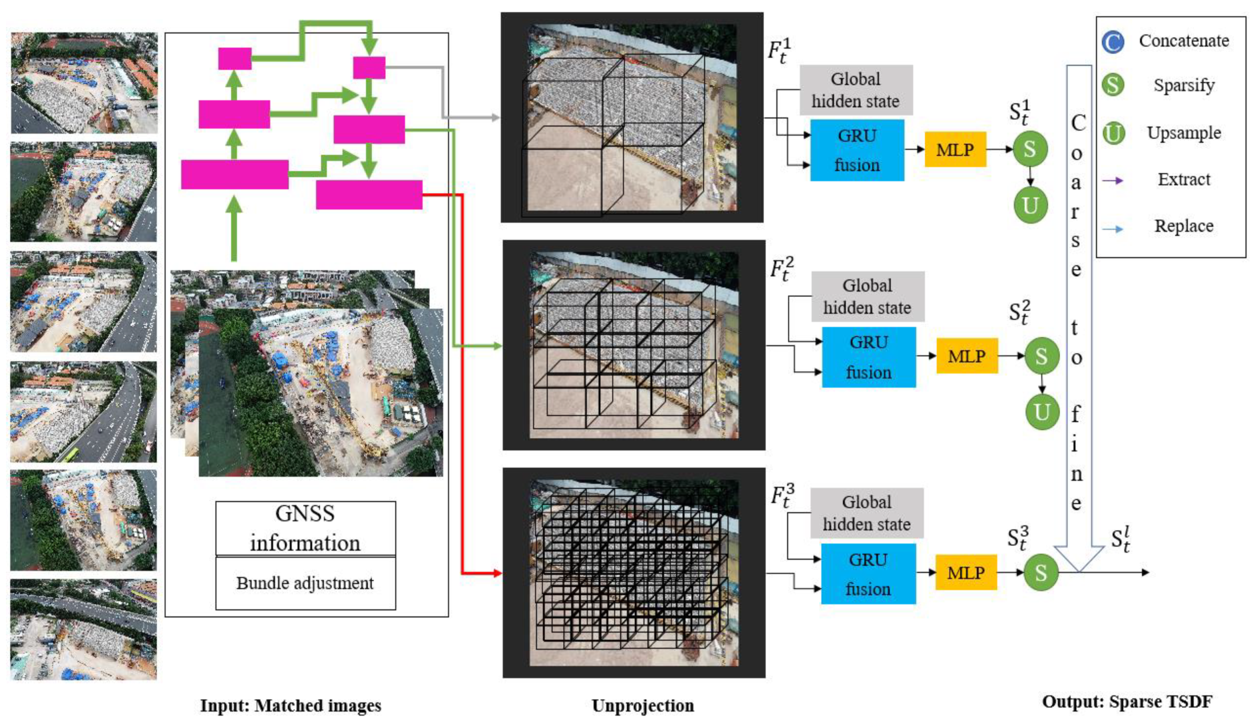
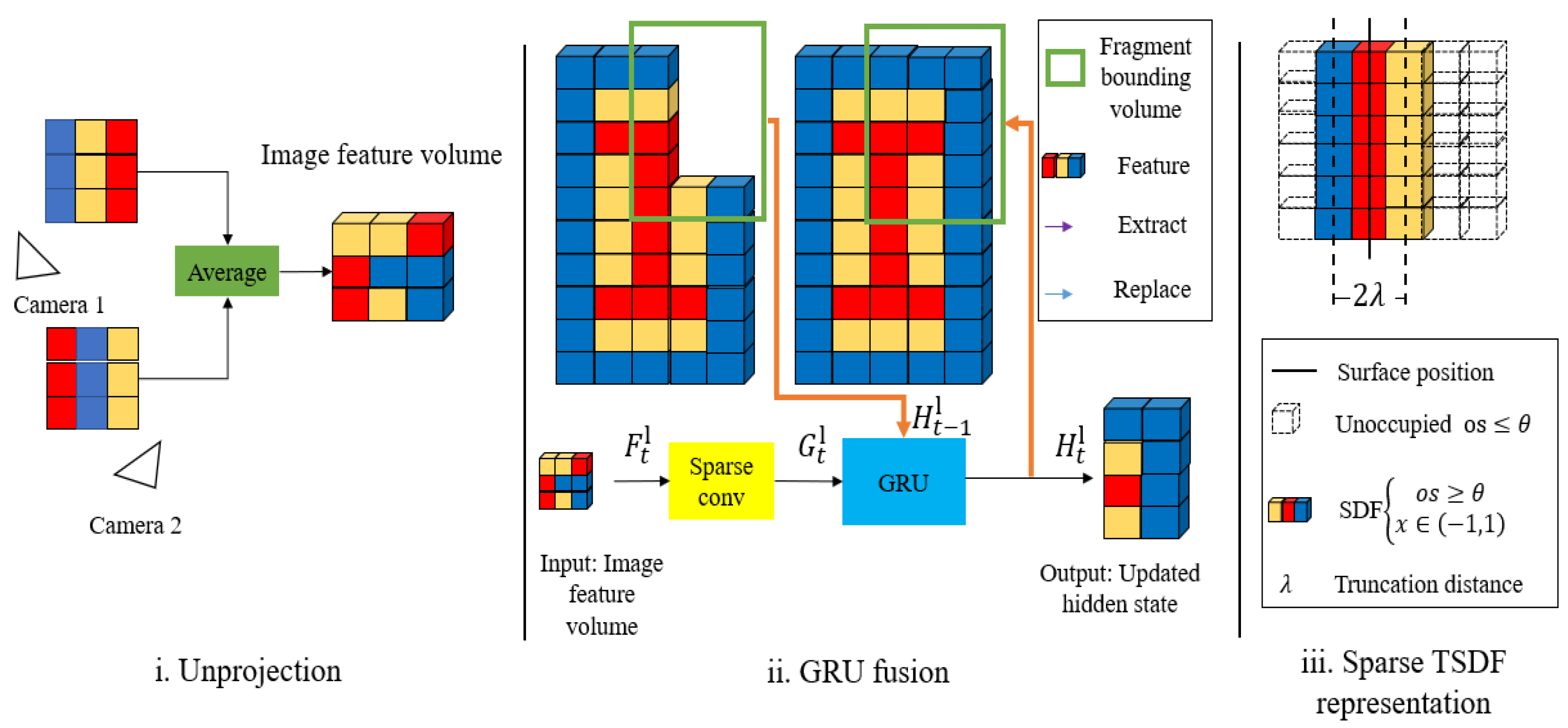
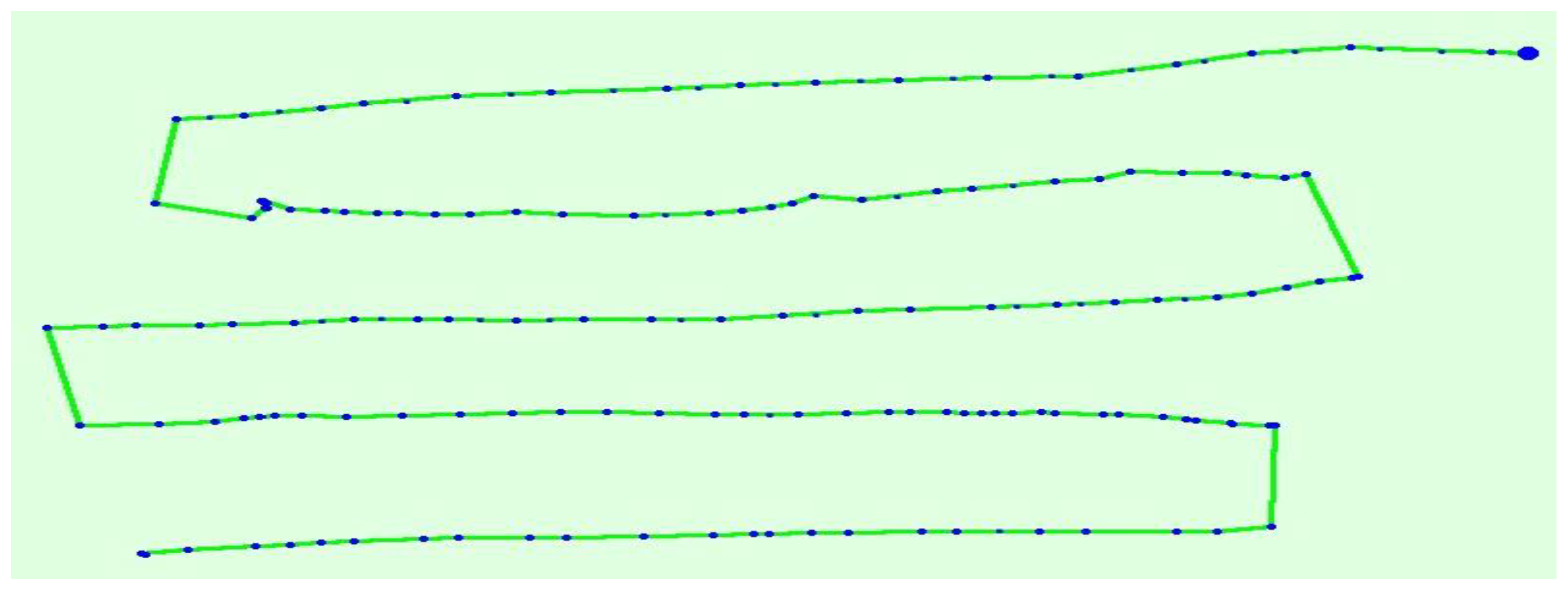
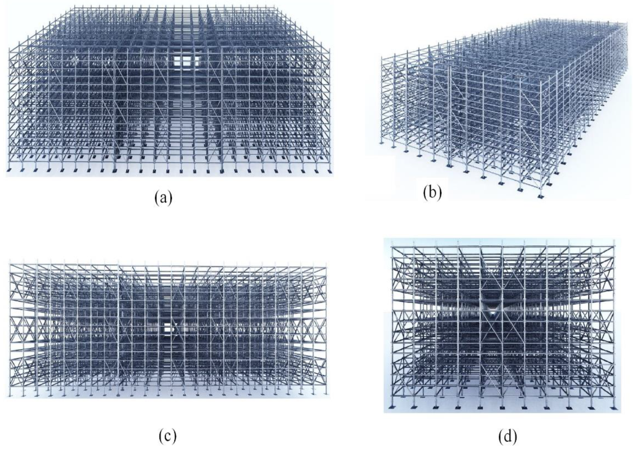
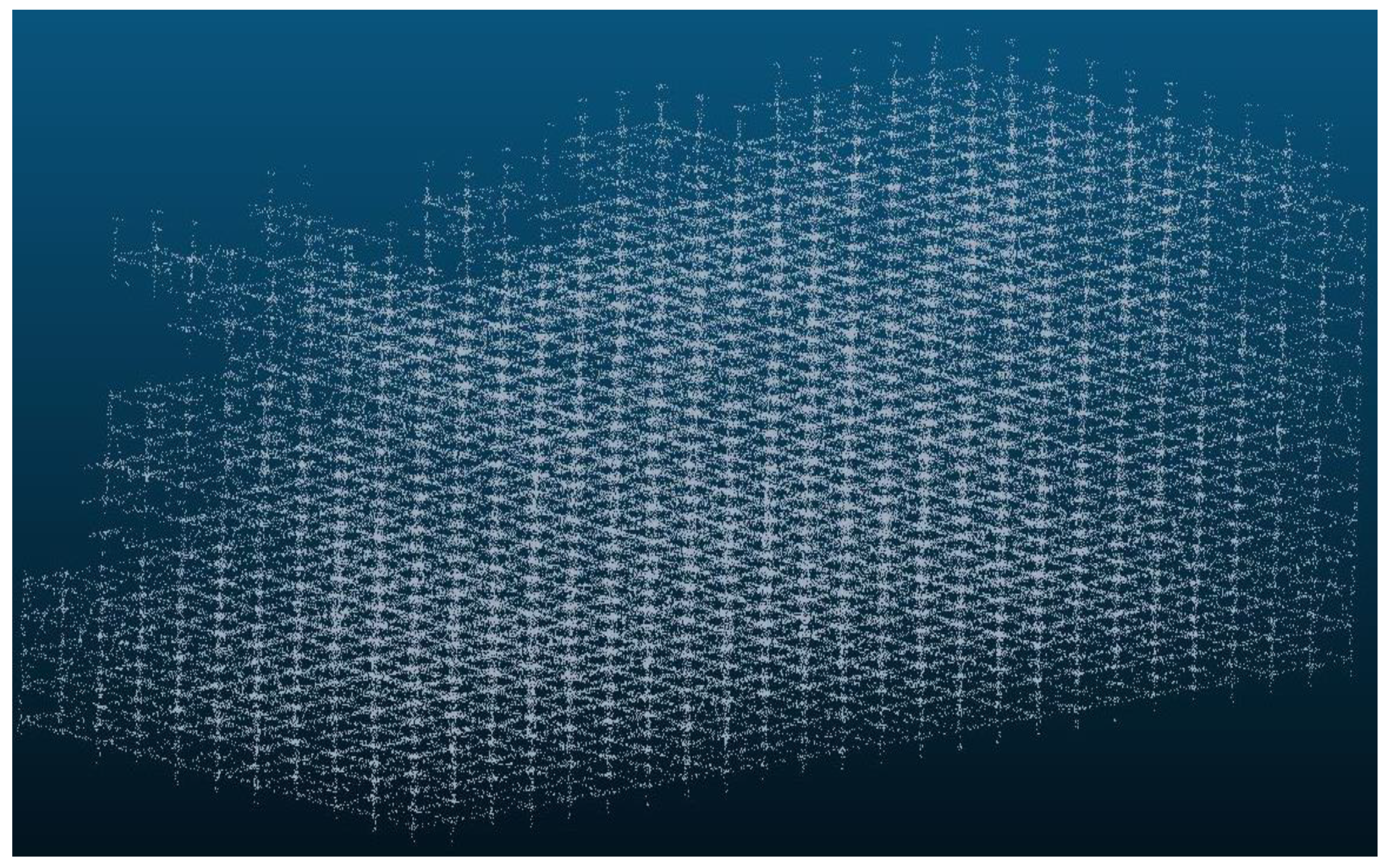
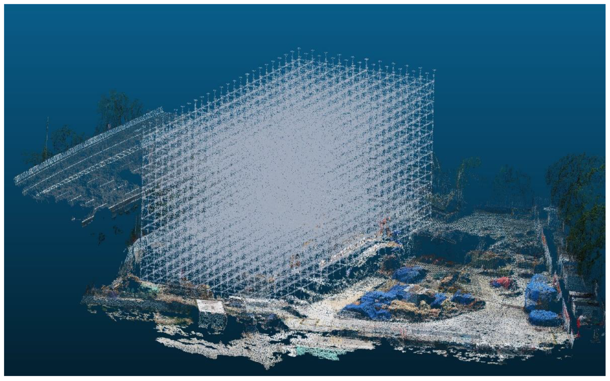
Table 1.
UAV data.
| Image | Altitude (m) | Distance (m) | Image Scale | |
|---|---|---|---|---|
| Nadir | 156 | 20–30 | 15–20 | 4600–6500 |
| Oblique | 83 | 10–20 | 10–15 | 5500–6800 |
| Overlap | Camera Angles | |||
| Camera images | 90/90 or 70/70 | Nadir + oblique camera angles |
Table 2.
Specifications and parameters for the TLS.
| Scanner Specifications | Leica Scan Station P50 |
|---|---|
| Scan rate | 976,000 points/s |
| Range | 0.6–120 m |
| Range error | 2 mm at 10 m (90% reflectivity) |
| Range noise | 0.6 mm at 10 m (90% reflectivity) |
| Total image resolution | Up to 70 Mpix |
Sourced from Leica document.
Table 3.
Laser scan data.
| Leica Scan Station P50 | |
|---|---|
| Stations | 6 |
| 3D points | 1,001,065 |
| Scan durations | 5 h |
| Mean resolution (mm) | 3–5 |
| Reg.prec.Register (mm) | 6 |
| Reg.prec.Cyclone(mm) | 4 |
Table 4.
Processing settings in Pix 4D mapper.
| Step | Overlap | Camera Angles |
|---|---|---|
| Initial processing | Keypoint image scale Matching image pairs Calibration | Full Aerial grid or corridor Standard ( camera self-calibration) |
| Point cloud densification | Image scale Point density Minimum number of matches Matching window size | Original image size (slow) Multiscale Optimal 4 9 9 pixels |
1 Automatic aerial triangulation (AAT); 2 Bundle block adjustment.
Table 5.
A summary of results of the different methods.
| Alignment | Photogrammetry | TLS | Data Fusion 1 | Data Fusion 2 |
|---|---|---|---|---|
| Total input data size | 2.74 G | 2.88 G | 5.6 G | 5.2 G |
| Number of registered images | 239/239 | 239/239 | 239/239 | |
| Number of registered laser scans | 6/6 | 6/6 | 6/6 | |
| Number of points | 1,804,180 | 1,001,065 | 2,805,245 | 2,504,328 |
| Metric scale | No | Yes | Yes | |
| Reconstruction | ||||
| Number of vertices | 15,328,689 | 13,306,254 | 27,025,188 | 23,058,878 |
| Number of faces | 31,058,214 | 27,258,687 | 55,557,121 | 51,028.339 |
Table 6.
RMSE errors of the check points for the data point clouds.
| Photogrammetry | TLS | Data Fusion 1 | Data Fusion 2 | |
|---|---|---|---|---|
| GCP RMSE (cm) | 14.9 | 2.5 | 13 | 5 |
Table 7.
Computing times for each model from pre-processed to textured mesh model.
| Image-Based | TLS | Data Fusion 1 | Data Fusion 2 | |
|---|---|---|---|---|
| Pre-processed time | 20 min | 2 h: 30 min | 3 h: 10 min | 30 min |
| Meshing time | 10 min | 2 h: 15 min | 3 h: 45 min | 3 h: 10 min |
| Texturing time | 10 min | 3 h: 20 min | 5 h: 10 min | 4 h |
| Total time | 40 min | 8 h: 05 min | 12 h: 05 min | 7 h: 40 min |
Table 8.
Summary of the image histogram analysis.
| Photogrammetry | TLS | Data Fusion 1 | Data Fusion 2 | |
|---|---|---|---|---|
| Mean | 71 | 111 | 100 | 81 |
| Std.dev. | 32 | 48 | 42 | 36 |
| Number of black pixels | 1436 | 1,768,325 | 4015 | 3867 |
| Number of white pixels | 1568 | 3,664,783 | 916,487 | 803,721 |
| Percentage of black pixels | 0.00089% | 1.02% | 0.0028% | 0.0019% |
| Percentage of white pixels | 0.00093% | 2.23% | 0.52% | 0.47% |
Disclaimer/Publisher’s Note: The statements, opinions and data contained in all publications are solely those of the individual author(s) and contributor(s) and not of MDPI and/or the editor(s). MDPI and/or the editor(s) disclaim responsibility for any injury to people or property resulting from any ideas, methods, instructions or products referred to in the content. |
© 2023 by the authors. Licensee MDPI, Basel, Switzerland. This article is an open access article distributed under the terms and conditions of the Creative Commons Attribution (CC BY) license (https://creativecommons.org/licenses/by/4.0/).
Share and Cite
MDPI and ACS Style
Zhao, L.; Zhang, H.; Mbachu, J. Multi-Sensor Data Fusion for 3D Reconstruction of Complex Structures: A Case Study on a Real High Formwork Project. Remote Sens. 2023, 15, 1264. https://0-doi-org.brum.beds.ac.uk/10.3390/rs15051264
AMA Style
Zhao L, Zhang H, Mbachu J. Multi-Sensor Data Fusion for 3D Reconstruction of Complex Structures: A Case Study on a Real High Formwork Project. Remote Sensing. 2023; 15(5):1264. https://0-doi-org.brum.beds.ac.uk/10.3390/rs15051264
Chicago/Turabian StyleZhao, Linlin, Huirong Zhang, and Jasper Mbachu. 2023. "Multi-Sensor Data Fusion for 3D Reconstruction of Complex Structures: A Case Study on a Real High Formwork Project" Remote Sensing 15, no. 5: 1264. https://0-doi-org.brum.beds.ac.uk/10.3390/rs15051264
Note that from the first issue of 2016, this journal uses article numbers instead of page numbers. See further details here.