

Efficient and Accurate Hierarchical SfM Based on Adaptive Track Selection for Large-Scale Oblique Images

School of Geographic and Environmental Sciences, Tianjin Normal University, Tianjin 300387, China
*
Author to whom correspondence should be addressed.
Remote Sens. 2023, 15(5), 1374; https://0-doi-org.brum.beds.ac.uk/10.3390/rs15051374
Submission received: 23 January 2023
/
Revised: 18 February 2023
/
Accepted: 26 February 2023
/
Published: 28 February 2023
(This article belongs to the Special Issue UAV Photogrammetry for 3D Modeling)
Abstract
:Image-based 3D modeling has been widely used in many areas. Structure from motion is the key to image-based reconstruction. However, the rapid growth of data poses challenges to current SfM solutions. A hierarchical SfM reconstruction methodology for large-scale oblique images is proposed. Firstly, match pairs are selected using positioning and orientation (POS) data and the terrain of the survey area. Then, images are divided to image groups by traversing the selected match pairs. After pairwise image matching, tracks are decimated using an adaptive track selection method. Thirdly, submaps are reconstructed from the image groups in parallel based on incremental SfM in the object space. A novel method based on statistics of the positional difference between common tracks is proposed to detect the outliers in submap merging. Finally, the reconstructed submaps are incrementally merged and optimized. The proposed methodology was used on a large oblique image set. The proposed methodology was compared with the state-of-the-art image-based reconstruction systems COLMAP and Metashape for SfM reconstruction. Experimental results show that the proposed methodology achieved the highest accuracy on the experimental dataset, i.e., about 22.37, and 3.52 times faster than COLMAP and Metashape, respectively. The experimental results demonstrate that the proposed hierarchical SfM methodology is accurate and efficient for large-scale oblique images.
1. Introduction
In recent years, image-based modeling based on oblique aerial images acquired by unmanned aerial vehicle (UAVs) has been widely used for urban planning, infrastructure monitoring, environmental monitoring, emergency response, and cultural heritage conservation [1,2,3,4,5,6,7,8]. The core techniques of image-based 3D reconstruction include image matching, structure from motion (SfM), and dense matching. Image matching extracts feature points from images and matches the feature points using similarity measures [9]. Tie points are then determined by filtering the matched feature points based on the fundamental matrix with a random sample consensus (RANSAC) framework [10]. Tracks are generated by connecting the geometrically consistent tie points. SfM is used to fully automatically orient the images and reconstruct a sparse model of a scene. The poses of images, spatial positions of tracks, and calibration parameters of cameras are globally optimized with bundle block adjustment [11]. Based on the sparse reconstruction, dense matching extracts dense correspondence between overlapping images and generates depth maps [12]. A dense point cloud is then derived by fusing the depth maps. Finally, a photorealistic 3D model is obtained by meshing the dense cloud and texturing the mesh with the acquired images. This pipeline works well in 3D modelling based on small-sized datasets. With fast-growing images, SfM has encountered challenges in terms of efficiency. [13].
Incremental SfM is well known in early studies for the reconstruction of landmarks based on photos collected from the Internet [14,15]. The incremental SfM firstly reconstructs an initial stereo model using a selected image pair, and then grows the model by iteratively adding new images and globally optimizing all parameters. The time complexity of the initial incremental SfM methodology is commonly known to be O(n4) for n images, which impedes the application of the initial incremental SfM on large datasets. Many studies have been proposed to reduce the complexity of incremental SfM. A methodology based on conjugate gradients was proposed in [16] to improve the efficiency of solving large-scale bundle problems. Experiments showed that the truncated Newton method, paired with relatively simple preconditioners, achieved a significant efficiency improvement on datasets containing tens of thousands of images. The incremental SfM pipeline was extended to reconstruct city-scale image collections [17]. The proposed pipeline was built on distributed algorithms for image matching and SfM. Each stage of the pipeline was fully parallelized. Experiments showed that the proposed pipeline was able to reconstruct a large scene with more than a hundred thousand unstructured images in less than a day. A novel methodology was proposed to improve the efficiency of the incremental SfM in [18]. A preemptive matching strategy was proposed to speed up the image matching process. Moreover, the multicore bundle block adjustment algorithm proposed in [19] was used to improve the efficiency of SfM. Experiments on large photo collections showed that the time complexity of the proposed pipeline was close to O(n).
Hierarchical SfM is a natural extension of the incremental strategy. It adopts the divide-and-conquer approach to improve the efficiency of SfM. A variety of hierarchical methodologies have been proposed. An out-of-core bundle adjustment was proposed for large-scale 3D reconstruction [20]. The proposed approach partitioned the cameras and points into submaps by performing graph-cut inference on the graph built from connected images and points. The submaps were reconstructed in parallel, and merged globally afterwards. The proposed methodology performed well on synthetic and real datasets. A hierarchical approach based on skeletal graphs was proposed for efficient SfM [21]. The proposed approach computed a small skeletal set of images using maximum leaf spanning tree. Then, it reconstructed the scene based on the skeletal set, and any remaining images were added using pose estimation. Experiments on datasets containing thousands of images showed that the methodology achieved dramatic speedups compared to the traditional incremental SfM. A hierarchical pipeline based on the cluster tree model was proposed [22,23,24]. Images of a scene were firstly organized to a hierarchical cluster tree. Then, the pipeline reconstructed the scene along the tree from the leaves to the root. Experiments on several datasets containing hundreds of images showed that increased speedup was achieved compared to Bundler and VisualSFM. A multistage approach for SfM reconstruction was proposed [25]. The approach firstly reconstructed a coarse model of a scene using a fraction of feature points. The coarse model was then completed by registering the remaining images and triangulating new feature points. Experiments showed that the proposed approach produced similar quality models as compared to Bundler and VisualSFM, while being more efficient. A hierarchical methodology with many novel techniques was proposed to systematically improve the performance of SfM reconstruction [26]. The proposed methodology partitioned the scene into many small, highly overlapping image groups. The image groups were reconstructed individually, and then merged together to form a complete reconstruction of the scene. The proposed pipeline reduced the runtime on a large dataset by 36% when the overlap ratio between two image groups was set as 40%. A similar hierarchical approach was proposed for large-scale SfM [27]. Images were firstly organized into a hierarchical tree using agglomerative clustering. Smaller image sets were reconstructed and merged in a bottom-up fashion. A scalable hierarchical SfM pipeline was proposed to process city-scale aerial images on a cluster of ten computers [28]. Images were clustered by graph division and expansion. The image clusters were reconstructed in an incremental manner. The reconstructed clusters were merged using robust motion averaging. The hybrid pipeline performed well in terms of robustness and efficiency. A novel methodology was proposed to systematically improve the performance of hierarchical SfM for large-scale image sets [29]. Images were clustered based on a dynamic adjustment strategy. Unreliable clusters were removed, and corresponding images were redistributed. Experiments on large terrestrial and aerial datasets demonstrated the robustness and efficiency of the pipeline. A hierarchical approach with a focus on cluster merging was proposed [30]. Images were divided into non-overlapping clusters via an undirected weighted match graph. The match graph was simplified with a weighted connected dominating set, and a global model was extracted. After parallel reconstruction, clusters were merged based on the extracted global model.
In addition to the above research directions, reducing the scale of a reconstruction problem becomes a noteworthy line of research. It improves the efficiency of SfM by reducing the number of parameters to be optimized in a reconstruction. An efficient pipeline based on image clustering and the local iconic scene graph was proposed [31]. Images were firstly clustered based on visual similarity. Then, local iconic scene graphs corresponding to city landmarks were extracted from the image clusters. The local iconic scene graphs were processed independently using an incremental approach. Experiments showed that the pipeline could reconstruct landmarks of a city based on millions of Internet images on a single workstation within a day. The preemptive matching strategy proposed in [18] only used only a proportion of top-scale SIFT feature points for image matching. This strategy significantly speeded up image matching. Furthermore, the efficiency of SfM was also improved as the estimated number of tracks was reduced. A reduced bundle adjustment model was proposed for oblique aerial photogrammetry [32]. The poses of oblique images were parameterized with the poses of nadir images and constant relative poses between oblique and nadir cameras. This approach significantly reduced the number of parameters and exhibited improvements in time and space efficiency. A track selection approach was proposed as a general technique for efficiency improvement [33]. A subset of tracks was selected in consideration of compactness, accurateness, and connectedness. Experimental results demonstrated that the efficiency of two open-source SfM solutions was improved using the track selection approach. A method for selecting building facade texture images from oblique images based on existing building models was proposed for photorealistic building model reconstruction [34]. Experimental results showed that the reconstruction process was significantly accelerated using the selected images. An oblique imagery selection methodology was proposed to improve the efficiency of SfM towards building reconstruction in rural areas [35]. Oblique images covering buildings were automatically selected out of a large-scale aerial image set using Mask R-CNN. The selected oblique images and all nadir images were used for SfM reconstruction and dense matching. The approach improved the efficiency of SfM while obtaining dense clouds of similar quality compared to the conventional pipeline. A performant hierarchical approach based on track selection was proposed [36]. The proposed approach firstly clustered the images based on their observation directions. Then, the tracks were selected based on a grid with a fixed spatial resolution. Submaps were sequentially reconstructed from the image clusters and merged. The hierarchical approach performed well on several large-scale datasets.
Although the above researches have made significant progresses in improving the efficiency of large-scale SfM, challenges still exist. In this paper, a hierarchical SfM pipeline based on an adaptive track selection approach is proposed for large-scale oblique images. Section 2 details the workflow and procedures of the proposed methodology. Experimental results and comparisons with two widely used solutions are detailed in Section 3. Discussions of the proposed methodology and the results are presented in Section 4. Conclusions are made in Section 5.
2. Methodology
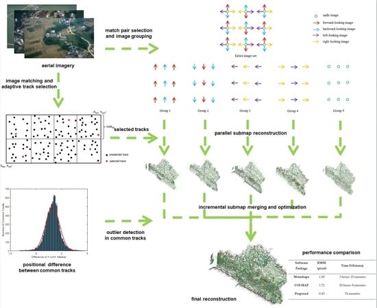
The workflow of the proposed methodology is illustrated in Figure 1. Firstly, match pair selection is performed on an aerial image set using positioning and orientation (POS) data and the terrain of the survey area. Based on the match pair selection, pairwise image matching and image grouping are carried out. Adaptive track selection based on track georeferencing is performed after pairwise image matching to decimate tracks. The image grouping procedure divides the images to non-overlapping image groups. Based on the selected tracks, parallel reconstruction is performed on the image groups to generate submaps using incremental SfM in the object space. A novel method is proposed to detect the outliers in common tracks between the reconstructed submaps. Finally, the reconstructed submaps are incrementally merged.
2.1. Image Grouping Based on Traversal of Match Pairs
The image grouping procedure exploits match pairs and divides the entire image set to non-overlapping groups which do not have common images. Match pairs define the overlapping relationship between images which is usually used for pairwise image matching. The match pair selection method proposed in [37] is used to generate match pairs in this study. The match pair selection process works as follows. Firstly, the principal point of each image is georeferenced using the acquired POS data and an existing elevation model of the survey area. Then, the overlapping relationship between images is determined based on the georeferenced principal points using the k-nearest neighbor search. In this study, seven match pairs are generated for each oblique image. These match pairs include two pairs from neighboring images acquired by the same camera, four pairs from neighboring images acquired by the camera looking at the opposite direction, and one pair from a neighboring nadir image. Four match pairs are generated for each nadir image. These match pairs include two pairs from neighboring nadir images in the same strip and two pairs from nadir images in the neighboring strips.
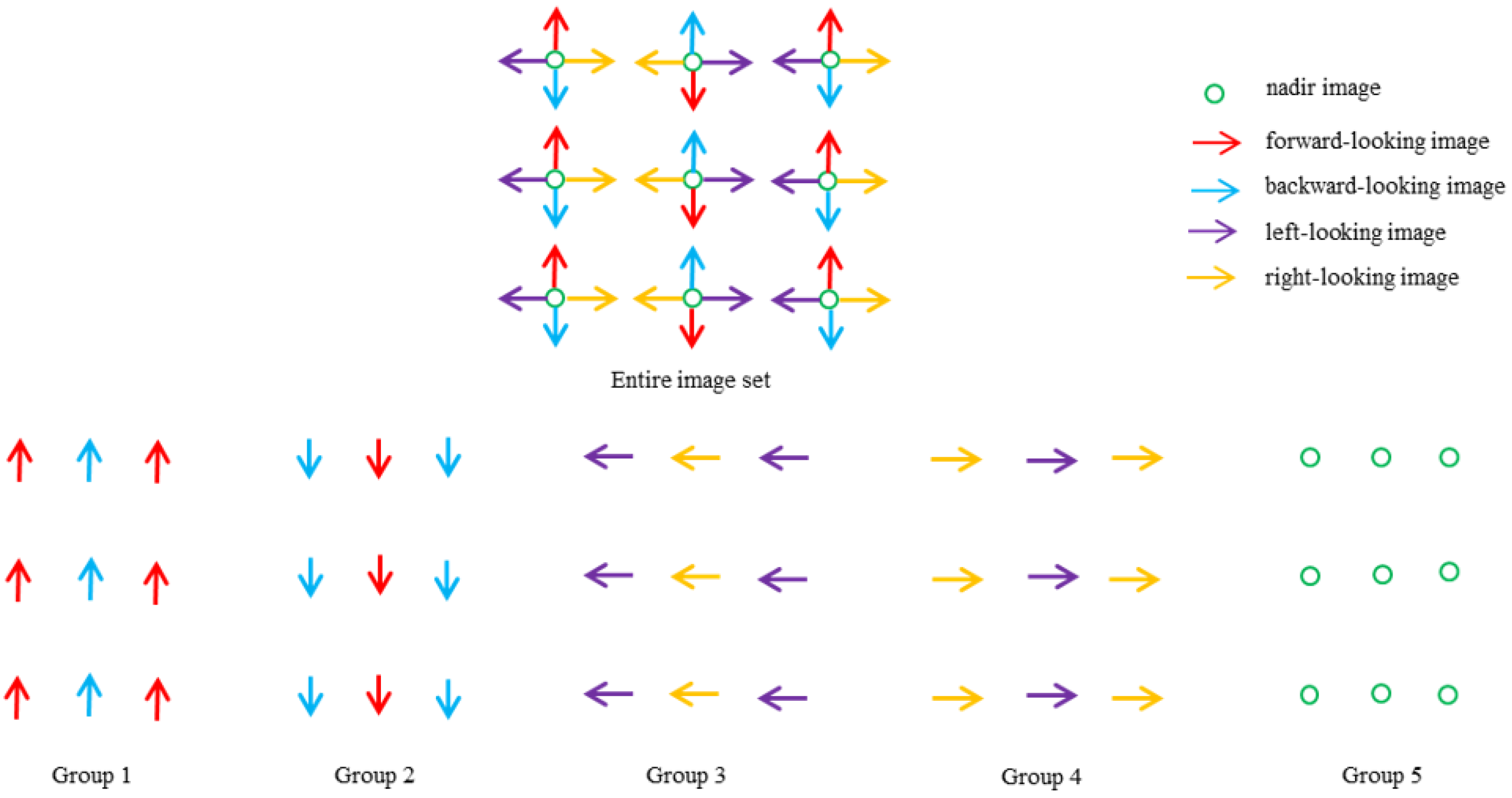
Based on the selected match pairs, the image grouping procedure divides the entire image set to five groups, as illustrated in Figure 2. The entire image set is composed of images in three strips. There are three exposure positions in each strip. At each exposure position, images acquired by five cameras looking at different directions are exposed simultaneously. These images are represented by colored arrows and circles. The observation direction of an image is represented by the direction of an arrow. It can be seen from the figure that the image grouping procedure divides the images according to their spatial proximity and similarity of observation directions. Images in each group have similar observation directions, and each image spatially overlaps with its neighbors.
The algorithm for the image grouping procedure is described by Algorithm 1. When the procedure meets an unprocessed match pair, a stack is initiated, and the images from the current match pair are added to the stack. Then, the procedure pops an image from the stack at a time, and adds it to the current group. The procedure finds its match pairs in the entire set of match pairs. For each one in the found match pairs, the procedure adds the matched image to the stack if the match pair has not been processed. The current growing process terminates until the stack is empty. The image grouping procedure traverses all the match pairs and divides the images to five groups, as illustrated in Figure 2.
| Algorithm 1 Image grouping by traversal of match pairs |
| Input: match pairs ; each pair specifies the match relationship between image i and j |
| Output: image groups |
| Initialization: |
| 1: for each pair in |
| 2: if is not processed |
| 3: initialize a new group |
| 4: initialize a stack , add and to |
| 5: while is not empty |
| 6: pop top element from , add to |
| 7: for each match pair in |
| 8: if is not processed |
| 9: push into |
| 10: end if |
| 11: end for |
| 12: end while |
| 13: add to |
| 14: end if |
| 15: end for |
| 16: return |
2.2. Adaptive Track Selection
Tracks correspond to 3D points in the object space. Tracks are generated from tie points which are determined by pairwise image matching. Pairwise image matching is carried out based on the result of the match pair selection. In this study, RootSIFT with the approximate nearest neighbor (ANN) algorithm is used to generate putative matches for each match pair. To speed up the matching process, the preemptive matching technique is used. Then, putative matches between two images are geometrically verified based on the fundamental matrix with RANSAC loops to generate tie points. Based on the geometrically verified tie points, the tracks are then generated.
To improve the efficiency of the following SfM reconstruction process, an adaptive track selection method is proposed. The adaptive track selection is performed on the generated tracks in the object space. The tracks are georeferenced to determine their positions in the object space, which is illustrated in Figure 3. For a given track, its image observations are determined by pairwise matching. Therefore, its 3D position can be estimated using its image observations and the orientation observations of corresponding images.
In this study, the position of a track is calculated as follows. Firstly, the position is solved based on each observation using the DEM-aided georeferencing of a single image. Secondly, the georeferencing positions are averaged to determine the final position of the track. The fundamental model of DEM-aided direct georeferencing is the inverse form of the collinearity equations as follows.
where is the spatial position of a track under the object coordinate system, is the image observation of the track under the image plane coordinate system, is the spatial position of the projection center under the object coordinate system, f is the focal length, and to are nine elements of the rotation matrix from the image space coordinate system to the object coordinate system.
The algorithm for the adaptive track selection procedure is described by Algorithm 2.
Basically, the procedure iteratively selects tracks until each image has no less than a minimum number of observations (MNO). To effectively decimate the tracks, the tracks with a large number of observations are preferable as they add more constraints. To select the tracks with a large number of observations, the track selection is conducted based on a series of 2D grids. Firstly, the range of the grids is determined based on the result of track georeferencing. Then, an initial ground sample distance () is calculated, and a grid is initialized. The tracks are mapped to the cells of the grid based on their 2D position. Then, the track with the maximum number of observations is selected from each cell of the grid. To guarantee that all the images reach the MNO, the track selection works in an iterative manner. In each iteration, the is halved and a new grid is generated with finer cells. The remaining tracks are mapped to cells of the new grid. The track with the maximum number of observations is selected from each cell.
| Algorithm 2 Adaptive track selection |
| Input: tracks , where each track stores its image observations; the value of ; the number of observations operator |
| Output: selected tracks |
| Initilization: |
| 1: for each track in |
| 2: georeference |
| 3: end for |
| 4: calculate |
| 5: initialize a set |
| 6: add all the images into |
| 7: initialize the ground sample distance |
| 8: while is not empty |
| 9: initialize 2D grid with |
| 10: for each track in |
| 11: if is in |
| 12: continue |
| 13: end if |
| 14: find the images to which is visible |
| 15: if |
| 16: continue |
| 17: end if |
| 18: find the cell in which lies |
| 19: if is occupied by another track and |
| 20: continue |
| 21: else |
| 22: stores in |
| 23: end if |
| 24: end for |
| 25: for each cell in grid |
| 26: add the track stored in to |
| 27: end for |
| 28: update according to |
| 29: |
| 30: end while |
| 31: return |
The initial of the grid is calculated according to Equation (3).
where and are the width and height of the ground projection of an image, respectively. The first two iterations of the track selection process are illustrated in Figure 4. Figure 4a shows the initialized grid with the initial . The points in the figure are the tracks mapped to the cells. The red point in each cell indicates the selected track with the maximum number of observations. Figure 4b shows the result of the second iteration. The is halved and the tracks with the maximum number of observations in the cells are selected.
2.3. Parallel Submap Reconstruction and Incremental Submap Merging
Based on the selected tracks, submaps are reconstructed from image groups in parallel. Each submap is reconstructed using incremental SfM in the object space. The optimization problem is formulated as a joint minimization of the sum of the squared reprojection errors and the sum of the squared positioning errors. The object function for the optimization is given by Equation (4).
where is an image observation of a 3D point on image j, represents the camera parameters of image j, is the function that projects a 3D point onto the image plane, denotes the L2-norm, is the position observation of image k, is the estimated position of image k, is an indicator function with = 1 if point is visible to image (otherwise, = 0). is a weight for the squared positioning errors, and it is calculated according to Equation (5).
where is the accuracy of image observations, while is the accuracy of the global navigation satellite system (GNSS) observations.
Common tracks between two submaps can be determined with ease as all submaps are reconstructed based on the same set of selected tracks. To detect the outliers in the common tracks between two submaps, the positional difference in common tracks is exploited. It can be assumed that and are estimated coordinates of two common tracks with the same index i. is taken from Submap 1 and is taken from Submap 2. It can be assumed that:
where is the true coordinate of the track, and are the residual errors corresponding to and , respectively. It can be assumed that and are subject to two normal distributions, as follows.
where and are the means of the distributions, while and are the variances in the distributions. The positional difference between and is given by Equation (10).
Based on the above assumptions, it can be deduced that is subject to the normal distribution given by Equation (11).
Based on the normal distribution of , the three-sigma rule is used to detect and remove outliers in the common tracks. Specifically, a pair of common tracks is determined as an outlier as long as the positional difference along an axe is outside the range of the corresponding mean value plus and minus three times the corresponding standard deviation.
After the detected outliers are removed from the common tracks, the submaps are incrementally merged. The submap reconstructed from the image group composed of nadir images is used as the base map. The other submaps are incrementally merged to the base map. To merge a submap, a similarity transformation is firstly estimated. For common tracks {} and {}, the transformation can be estimated by minimizing the object function given by Equation (12).
where is the rotation matrix, is the translation vector, is the scaling factor, and is the Huber loss function. denotes the L2-norm.
Then, the estimated transformation is applied to the submap. The transformed submap is locally optimized with common tracks fixed to their counterparts in the base map. After merging the submap and the base map, the merged map is globally optimized and used as the base map for merging the next submap. For the local and global optimization, the problem for refining camera poses and 3D tracks is formulated to minimize the first term of Equation (4), where the sum of squared errors between the tie point observations and projections of the corresponding tracks is minimized.
3. Experimental Results
A large-scale aerial image set was used to evaluate the performance of the proposed methodology. Firstly, the specification of data acquisition is detailed. Secondly, the experimental results including image grouping, track selection, submap reconstruction, and merging are presented. Finally, the proposed methodology is compared with widely used software packages to demonstrate its performance. The proposed methodology was implemented in the C++ programming language. In this study, pairwise image matching, track generation, and bundle block adjustment were based on the open-source software OpenMVG [38]. Optimization problems were solved using the open-source software Ceres Solver [39]. All of the experiments were performed on a Dell Precision Tower 7810 workstation. The workstation was equipped with a Windows 10 Professional operating system, an Intel Xeon E5-2630 CPU (20 cores, 2.2 GHz), a NVIDIA Quadro M4000 GPU, and a 128 GB memory.
3.1. Survey Area and Data Specification
The dataset was acquired from a survey area mainly covered by farmland and vegetation. This area is 5.2 km from east to west and 4.1 km from south to north. The elevation of the area is about 65 m above the sea level. The terrain of the area is basically flat. Figure 5 shows an orthophoto of the survey area. The orthophoto was derived from the acquired images.
The area was surveyed in autumn 2018 with a five-camera imaging system mounted on a vertical take-off and landing (VTOL) fixed-wing UAV. Specifications of the data acquisition system are listed in Table 1.
The acquired positioning observations include latitude, longitude, and altitude which are defined under the World Geodetic System (WGS84). These observations were acquired based on the differential GNSS technique. No ground reference station was used during the surveying campaign. The accuracy of the GNSS observations was at the level of meters. The orientation observations, including omega, phi, and kappa, defined the sequential rotations around the X-Y-Z axes of the object coordinate system. In this study, the east–north–up (ENU) coordinate system was used as the object coordinate system. Figure 6 shows the position of exposures in the survey area. At each point, five images were synchronously exposed. The image acquisition started from the red point at the top of the area and finished at the blue point at the bottom. A total of 9775 images were acquired at 1955 exposure positions. Figure 7 shows the two sample images.
3.2. Pairwise Matching and Image Grouping
A total of 33,297 match pairs were selected. Based on the selected match pairs, pairwise image matching was performed. A total of 32,050 pairs were robustly matched with geometric verification, which accounted for 96.3% of all the selected match pairs. The number of robustly matched pairs and the selected match pairs are listed in Table 2. It can be seen from the table that almost all of the matched pairs from each single camera were robustly matched. The percentages of matched backward–forward and right–left image pairs were 95.0% and 97.0%, respectively. Although the percentage of matched oblique-nadir pairs was lower than that of the oblique–oblique ones, it was still higher than 87.1%. The pairwise image matching result shows that the oblique and nadir images were well connected.
Image grouping was also performed based on the selected match pairs. The procedure automatically divided the aerial images to five groups. Each group contained 1955 images. The first two groups contained images from the backward and forward cameras. The third and fourth group contained images from the left and right cameras. The last group only contained the nadir images.
3.3. Track Selection
A total of 1,137,945 tracks were directly generated based on the result of pairwise image matching. Table 3 lists the statistics of track length and image observations. The length of a track was the total number of its image observations. The observations of an image corresponded to the total number of tracks visible to the image. The maximum track length was 130, which means the corresponding track was observed in 130 images. The median and mean of track length were less than 7, which demonstrates that most tracks could only be observed in a few images. The standard deviation of the track length indicates that most tracks had a similar number of observations. The second row of the table shows that the maximum and minimum of image observations differed significantly. It is found that the image with zero track observations was largely covered by water. The image procedure failed to match this image with other ones, meaning that it had no track observations. There were more than 700 observations in an image on average. The standard deviation shows that the number of observations varied greatly among the images.
After track georeferencing, the positions of the tracks in the object space were determined. In this study, an ASTER GDEM2 elevation model of the survey area was used to georeference the tracks. The ASTER GDEM2 elevation model was downloaded from USGS EarthExplorer as a GeoTIFF image. The resolution of the image was 3601 by 3601 pixels. The spatial resolution of the elevation model was about 30 m. The ASTER GDEM2 elevation model refers to WGS84 with the height values transformed via the EGM96 model to the physical height. The vertical accuracy of the elevation model is about 15.85 m [40]. Figure 8 shows the georeferenced tracks. The tracks were colored according to their length. It can be seen from Figure 8a that the tracks less than 11 in length covered the whole survey area. The density of longer tracks was lower than that of the shorter ones. It can be found by combining Figure 5 and Figure 8 that long tracks were mainly located in the areas covered by bare earth or buildings. The feature points extracted in the areas covered by farm field were less repetitive. The experimental results demonstrate that a large track length was highly corelated with land cover.
Adaptive track selection was performed based on the track georeferencing results. Figure 9 shows the relationship between the MNO value and the number of selected tracks. The figure demonstrates that the number of selected tracks was linearly correlated with the MNO.
Table 4 lists the length statistics of the adaptively selected tracks with various MNO values. It can be seen that the mean and median track length of selected tracks decreased with increasing MNO values. As is shown by Figure 8, there were fewer longer tracks than shorter ones. With the increase in the MNO, more and more shorter tracks were selected. As a result, the mean track length and the median track length decreased. However, the values in the column of mean track length were much larger than the value listed in Table 3, which demonstrates that tracks with a large number of observations were effectively selected. The values in the column of standard deviation were also much larger than the counterpart listed in Table 3, which also demonstrates that longer tracks were selected with priority.
Table 5 lists the statistics of image observation based on adaptive track selection. All the indicators in the table were positively proportional to MNO values. It can be seen that the maximum, mean, and media values were smaller than their counterparts from Table 3, which means that the proposed track selection method effectively reduced the number of image observations on the whole. The standard deviation was also smaller than that from Table 3, which indicates that the number of observations became more balanced among the images.
Figure 10 shows the histograms of image observations of all tracks and the adaptively selected tracks. It can be seen from Figure 10a that the number of observations of most images ranged between 400 and 1200. However, there were still a considerable number of images on the left and right sides of the histogram. This means that the number of observations was unbalanced among the images. In comparison, the histogram of adaptively selected tracks shows that most images were concentrated in the range between 100 and 300. The smaller range visually demonstrates that the number of observations was more balanced among the images.
Figure 11 shows the selected tracks with the MNO set as 50. It can be seen that there were much fewer tracks in Figure 11a than in Figure 8a. It can be found that long tracks were complementary in space to the short ones. This is because long tracks were selected with priority. If the images met the MNO threshold given the selected long tracks, no other tracks were selected. On the contrary, more short tracks were selected in the areas where few long tracks existed. The selected tracks with the MNO set as 50 were used for the following experiments.
3.4. Submap Reconstruction and Merging
Based on the selected tracks and the five image groups, five submaps were reconstructed in parallel. The parallel reconstruction of submaps was implemented using multiple processes. For the reconstruction of a submap, bundle block adjustment was performed every time 30 images were added. Statistics of the reconstructed submaps are listed in Table 6. It can be seen that four reconstructions registered all the images. There were eight unregistered images in Submap 1. It is found that these images were largely covered by water. In addition, there were few matched feature points in these images. The number of reconstructed tracks in the submaps was comparable. However, the average length of tracks and average number of image observations in the submap reconstructed from the nadir images were larger than those in the submaps reconstructed from the oblique images. This indicates that tracks were more observable in the nadir images than in the oblique images. All the submap reconstructions achieved sub-pixel accuracy.
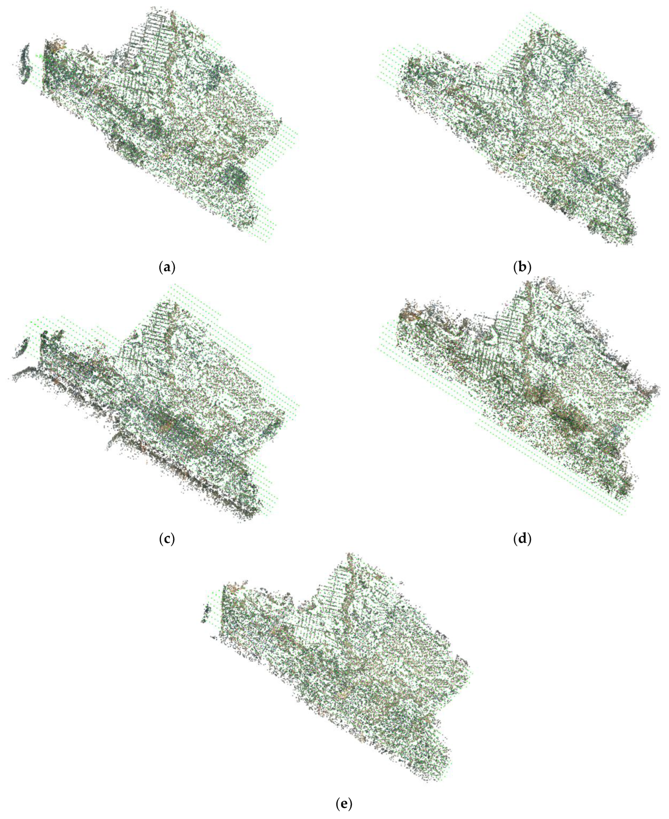
Figure 12 shows oriented images and reconstructed tracks for each reconstructed submap. The oriented images were labelled with green points. The color of the tracks was derived from corresponding image observations. The relative positions between oriented images and reconstructed tracks in the figures were different, which is due to the different observation directions of images. The experimental results show the effectiveness of the proposed method for image grouping.
Outliers in common tracks were detected based on the statistics of positional differences. The statistics of positional differences between common tracks of the reconstructed submaps are listed in Table 7. The numbers of common tracks between Submaps 1–5 and 2–5 were comparable. The numbers of common tracks between Submaps 3–5 and 4–5 were similar. The forward and backward submaps had more common tracks with the nadir submaps than the right and left submaps. This demonstrates that the image observations acquired by the forward and backward cameras were more similar to those acquired by the nadir camera. The average values of the positional differences along XYZ axes were at the level of meters, which indicates that there was a positional bias of meters between the reconstructed submaps. Most of the standard deviations of the positional differences along XYZ axes were at the level of meters. The standard deviations and average values show that most of the common tracks between an oblique submap and the nadir submap were close in space. The maximum and minimum of positional differences along XYZ axes were at the level of hundreds of meters, which were far from the corresponding mean values. This indicates the existence of outliers in the common tracks.
Figure 13 shows the positional difference histograms of common tracks between Submaps 1 and 5 within the range of mean values plus and minus three times the corresponding standard deviations. The red curves in the histograms were fitted normal distributions. It can be seen that the normal distributions fitted well with the histograms, which demonstrates the correctness of the proposed model for outlier detection.
The common tracks are visualized in Figure 14. The inliers and outliers were labeled with green and red points, respectively. In total, 91, 91, 79, and 97 outliers were detected in common tracks between Submaps 5-1, 5-2, 5-3, and 5-4, respectively. It can be seen from the figure that the outliers were more likely to be in the areas covered by road, farm field, and bare earth. There were fewer outliers detected in the building-covered areas. This is because feature points in these areas are more distinctive.
Figure 15 shows the image observations of an outlier detected in common tracks between Submaps 1 and 5. The observations were labelled with red circles in the images. Figure 15a,b are from the image group used to reconstruct Submap 1. Figure 15c,d are from the image group used to reconstruct Submap 5. It can be seen that the outlier was derived from corresponding outliers remaining in the matches. This demonstrates that although image matches were geometrically verified, the classical robust image matching technique could not remove all the outliers from the matches.
Statistics of incremental submap merging are listed in Table 8. A total of 102,148 tracks were reconstructed after merging all the submaps, accounting for 98.3% of the selected tracks. The high reconstruction ratio demonstrates the effectiveness of the proposed track selection method. The number of registered images shows that all of the images oriented in the submaps were successfully registered in the merging process. Sub-pixel accuracy was achieved in the process of merging each submap. This demonstrates that the accuracy of the final map was comparable to the accuracy of the submaps listed in Table 6, which indicates that errors did not accumulate in the submap merging process.
Figure 16 visualizes the incremental submap merging. The figure shows oriented images and a sparse point cloud after each submap was merged. The oriented images were labelled with green points. The figures visually demonstrate the robustness and accuracy of the proposed methodology.
3.5. Comparison with Software Packages
The proposed methodology was compared with two software packages that are widely used by the academic community and industry professionals. The software packages and their configurations are listed in Table 9.
Metashape is a commercial software package widely used by industry professionals and the research community for processing aerial images and producing orthomosaics, digital elevation models, and photorealistic 3D models [41]. It supports position-based and visual-similarity-based match pair selection. The ground altitude of the survey area was set as 65 m to make the position-based match pair selection procedure work efficiently. The visual-similarity-based match pair selection procedure finds overlapping images by matching the downscaled copies of original images. The software package parallelizes image matching using multi-core CPU and GPU. The software package exploits a hierarchical strategy for SfM reconstruction. The other parameters were set as default values.
COLMAP is an open-source software package widely used by the research community for image matching, sparse reconstruction, and dense reconstruction [26]. Match pair selection based on position was used for the experiments. The search radius and number of neighbors for the position-based match pair selection were set as 300 m and 150, respectively. To speed up the pairwise image matching process, down-sampled images were used for the experiments. Image matching in the software package was accelerated using multi-core CPU and GPU. Both incremental and hierarchical strategies for SfM reconstruction were available in the software package. In this study, the hierarchical strategy was used for experiments. Bundle block adjustment was performed every time 30 images were added. The other parameters were set as default values.
The same dataset was processed with the software packages mentioned above. The experimental results of SfM reconstruction are listed in Table 10. It can be seen that both Metashape and COLMAP registered all of the aerial images, which showed the robustness of these software packages. Metashape reconstructed about nine millions of tracks at the cost of about three hours of processing time. COLMAP reconstructed more than four millions of tracks, while its time efficiency was much lower than Metashape. Both software packages achieved pixel-level accuracy in the reconstructions. In comparison, the proposed methodology reconstructed the scene in less than an hour based on the adaptively selected tracks. It was about 22.37 and 3.52 times faster than COLMAP and Metashape, respectively. Specifically, the proposed methodology spent 15 s, 11 min, 19 min, and 23 min on image grouping, adaptive track selection, submap reconstruction, and submap merging, respectively. Reconstructing the five submaps took 19, 18, 11, 12, and 15 min, respectively. The proposed methodology was the most accurate on the experimental dataset. According to the basic principle of adjustment computation, assumed observations are independent and of the same accuracy, and more observations lead to more accurate estimation. However, the proposed method achieved more accurate estimation with far less image observations. This means that images observations were not of the same accuracy. The key is the number of redundant observations. As shown by Table 4, the selected tracks had a large number of redundant observations. For a single track, more redundant observations generally led to more accurate estimation. This is because less accurate observations and outliers could be effectively detected and removed with the help of a large number of redundant observations during the optimization of a scene. As a result, the accuracy of the image observations improved on the whole. Furthermore, more accurate image observations generally led to more accurate SfM reconstruction. To the best of our knowledge, Metashape and COLMAP did not force a threshold of minimum number of observations on tracks. A significant number of tracks with a few, and even no, redundant observations were reconstructed during SfM. In this situation, it was difficult to detect less accurate observations and outliers, reducing the overall accuracy of the image observations. Consequently, the SfM reconstruction was less accurate, although many more image observations were used.
4. Discussion
The proposed image grouping method is based on match pair selection and requires precision in the selected match pairs. The used match pair selection method generated match pairs using the position of images, the observation directions of images, and the terrain of the survey area. The pair-wise image matching results show that the generated match pairs are precise. The proposed image grouping method exploits the structure underlying an aerial survey which is generally based on regularly distributed exposures located in the parallel strips. The regularity of exposure also guarantees that images are acquired by two oblique cameras with opposite observation directions that overlap well with each other. The grouping procedure divides the images to non-overlapping groups instead of overlapping groups. This strategy avoids setting the overlapping ratio parameter which defines the ratio of images that two overlapping groups have in common. If the overlapping ratio parameter is set too high, the size of the generated image groups will increase. The efficiency of the submap reconstruction and merging will decrease. If the ratio parameter is set too low, the common images must lie at the boundary of the image groups. Then, the robustness and the accuracy of the submap reconstruction and merging will probably decrease as the estimated orientations of images at the boundary of an image network are generally of low accuracy.
The proposed method iteratively selects tracks using a series of 2D grids. The proposed method uses a series of grids instead of a single grid with a constant GSD for several reasons. Experimental results have shown that the density of tracks is highly correlated with the land cover of the survey area. It can be expected that the number of observations of an image acquired over a building-covered area is larger than that of an image acquired over a farm field. If a grid with a large GSD is used for track selection, images acquired over a farm field may fail in registration due to the lack of sufficient observations. If a grid with a small GSD is used, the efficiency of reconstruction will decrease as a large number of tracks are selected. On the contrary, the proposed method iteratively selects tracks until all images reach the MNO threshold. The MNO threshold is more meaningful than a constant GSD for image registration as the robustness of registration generally depends on the number of observations. Moreover, the iteratively halved GSD makes the track selection process converge fast as the number of selected tracks theoretically quadruples in each iteration. Therefore, the proposed iterative track selection method is effective and efficient.
As the selected tracks are used by the reconstruction of submaps, common tracks between the reconstructed submaps can be determined without difficulty. To detect outliers in the common tracks, the three-sigma rule is performed based on the positional difference in the common tracks. The proposed outlier detection method insists that the submaps are reconstructed in the object space. The experiments show that the proposed outlier detection model fits well with the data. The detected outliers show that the classical robust image matching technique cannot remove all the outliers from the matches. Image matching techniques taking into account relationship among feature points could be used to solve this problem.
Five submaps were reconstructed in parallel from corresponding image groups. The experimental results show the high performance of the parallel reconstruction. Although the image groups could be further divided to smaller ones, the time efficiency of the submap reconstruction might not be further improved as CPU usage had already approached 100% during the experiments. The nadir submap reconstructed from the nadir images was the only submap that had common tracks with the other four submaps. Moreover, Figure 6 shows that the mean track length and mean image observations of the nadir submap were larger than those of the oblique submaps, which indicates that the image network of the nadir submap was more stable than that of the oblique submaps. Therefore, the nadir submap was used as the base map during the submap merging process in favor for its stable network and high connectivity. The accuracy of the final map reflects the high inner consistency of the proposed submap merging method. However, the proposed submap merging method was suboptimal as the oblique submaps were optimized with common tracks fixed to their positions in the nadir submap. The absolute positioning accuracy of the final map will be systematically investigated in future work.
5. Conclusions
As a core technique, SfM is crucial for the accuracy, robustness, and efficiency of the image-based 3D modelling pipeline. A hierarchical SfM reconstruction methodology for large-scale oblique images is proposed in this paper. Based on match pair selection, images were divided into five image groups. After pairwise image matching, tracks were decimated using the adaptive track selection method. Then, incremental SfM was performed on the image groups in parallel to generate submaps in the object space. The three-sigma rule was performed on the positional difference between common tracks to detect the outliers. Finally, the reconstructed submaps were incrementally merged. The proposed methodology was experimented on a large dataset. Experimental results of the proposed methodology were fully explored. The proposed methodology was compared with COLMAP and Metashape. The experimental results reveal that the proposed methodology outperformed the software packages in terms of accuracy and efficiency. The experimental results demonstrate that the proposed hierarchical SfM methodology was accurate and efficient for large-scale oblique images.
Author Contributions
Conceptualization, Y.L.; methodology, Y.L.; software, Y.L.; validation, Y.L., X.F. and Y.Y.; formal analysis, Y.L.; investigation, Y.L.; resources, T.C.; data curation, Y.L. and X.F.; writing—original draft preparation, Y.L.; writing—review and editing, Y.L.; visualization, Y.L. and X.F.; project administration, Y.L.; funding acquisition, Y.L. All authors have read and agreed to the published version of the manuscript.
Funding
This research was jointly funded by the Special Foundation for the National Science and Technology Basic Research Program of China (No. 2019FY202500) and the Chinese National Nature Science Foundation (No. 41971410).
Data Availability Statement
The data presented in this study are available on request from the corresponding authors.
Conflicts of Interest
The authors declare no conflict of interest.
References
- Colomina, I.; Molina, P. Unmanned aerial systems for photogrammetry and remote sensing: A review. ISPRS J. Photogramm. Remote Sens. 2014, 92, 79–97. [Google Scholar] [CrossRef] [Green Version]
- Nex, F.; Armenakis, C.; Cramer, M.; Cucci, D.A.; Gerke, M.; Honkavaara, E.; Kukko, A.; Persello, C.; Skaloud, J. UAV in the advent of the twenties: Where we stand and what is next. ISPRS J. Photogramm. Remote Sens. 2022, 184, 215–242. [Google Scholar] [CrossRef]
- Haala, N.; Kada, M. An update on automatic 3D building reconstruction. ISPRS J. Photogramm. Remote Sens. 2010, 65, 570–580. [Google Scholar] [CrossRef]
- Duarte, D.; Nex, F.; Kerle, N.; Vosselman, G. Detection of seismic façade damages with multi-temporal oblique aerial imagery. GIScience Remote Sens. 2020, 57, 670–686. [Google Scholar] [CrossRef]
- Giordan, D.; Hayakawa, Y.; Nex, F.; Remondino, F.; Tarolli, P. Review article: The use of remotely piloted aircraft systems (RPASs) for natural hazards monitoring and management. Nat. Hazards Earth Syst. Sci. 2018, 18, 1079–1096. [Google Scholar] [CrossRef] [Green Version]
- Vetrivel, A.; Gerke, M.; Kerle, N.; Nex, F.; Vosselman, G. Disaster damage detection through synergistic use of deep learning and 3D point cloud features derived from very high resolution oblique aerial images, and multiple-kernel-learning. ISPRS J. Photogramm. Remote Sens. 2018, 140, 45–59. [Google Scholar] [CrossRef]
- Fernández-Hernandez, J.; González-Aguilera, D.; Rodríguez-Gonzálvez, P.; Mancera-Taboada, J. Image-based modelling from unmanned aerial vehicle (uav) photogrammetry: An effective, low-cost tool for archaeological applications. Archaeometry 2015, 57, 128–145. [Google Scholar] [CrossRef]
- Nex, F.; Remondino, F. UAV for 3D mapping applications: A review. Appl. Geomat. 2014, 6, 1–15. [Google Scholar] [CrossRef]
- Lowe, D.G. Distinctive image features from scale-invariant keypoints. Int. J. Comput. Vis. 2004, 60, 91–110. [Google Scholar] [CrossRef]
- Hartley, R.; Zisserman, A. Multiple View Geometry in Computer Vision, 2nd ed.; Cambridge University Press: Cambridge, UK, 2004. [Google Scholar]
- Gerke, M.; Nex, F.; Remondino, F.; Jacobsen, K.; Kremer, J.; Karel, W.; Hu, H.; Ostrowski, W. Orientation of oblique airborne image sets-experiences from the ISPRS/EUROSDR benchmark on multi-platform photogrammetry. Int. Arch. Photogramm. Remote Sens. Spat. Inf. Sci. 2016, XLI-B1, 185–191. [Google Scholar] [CrossRef] [Green Version]
- Hirschmüller, H. Stereo Processing by Semiglobal Matching and Mutual Information. IEEE Trans. Pattern Anal. Mach. Intell. 2008, 30, 328–341. [Google Scholar] [CrossRef] [PubMed]
- Jiang, S.; Jiang, C.; Jiang, W. Efficient structure from motion for large-scale UAV images: A review and a comparison of SfM tools. ISPRS J. Photogramm. Remote Sens. 2020, 167, 230–251. [Google Scholar] [CrossRef]
- Snavely, N.; Seitz, S.M.; Szeliski, R. Photo tourism: Exploring photo collections in 3D. ACM Trans. Graph. 2006, 25, 835–846. [Google Scholar] [CrossRef] [Green Version]
- Snavely, N.; Seitz, S.M.; Szeliski, R. Modeling the world from internet photo collections. Int. J. Comput. Vis. 2008, 80, 189–210. [Google Scholar] [CrossRef] [Green Version]
- Agarwal, S.; Snavely, N.; Seitz, S.M.; Szeliski, R. Bundle Adjustment in the Large. In Proceedings of the ECCV 2010, Crete, Greece, 5–11 September 2010; pp. 29–42. [Google Scholar]
- Agarwal, S.; Furukawa, Y.; Snavely, N.; Simon, I.; Curless, B.; Seitz, S.M.; Szeliski, R. Building rome in a day. Commun. ACM 2011, 54, 105–112. [Google Scholar] [CrossRef]
- Wu, C. Towards linear-time incremental structure from motion. In Proceedings of the International Conference on 3D Vision (3DV), Seattle, DC, USA, 29 June–1 July 2013; pp. 127–134. [Google Scholar]
- Wu, C.; Agarwal, S.; Curless, B.; Seitz, S.M. Multicore bundle adjustment. In Proceedings of the CVPR 2011, Colorado Springs, CO, USA, 20–25 June 2011; pp. 3057–3064. [Google Scholar]
- Ni, K.; Steedly, D.; Dellaert, F. Out-of-Core bundle adjustment for large-scale 3D reconstruction. In Proceedings of the ICCV 2007, Rio de Janeiro, Brazil, 14–21 October 2007; pp. 1–8. [Google Scholar]
- Snavely, N.; Seitz, S.M.; Szeliski, R. Skeletal graphs for efficient structure from motion. In Proceedings of the CVPR 2008, Anchorage, AK, USA, 23–28 June 2008; pp. 1–8. [Google Scholar]
- Farenzena, M.; Fusiello, A.; Gherardi, R. Structure-and-motion pipeline on a hierarchical cluster tree. In Proceedings of the ICCV 2009, Kyoto, Japan, 27 September–4 October 2009; pp. 1489–1496. [Google Scholar]
- Gherardi, R.; Farenzena, M.; Fusiello, A. Improving the efficiency of hierarchical structure-and-motion. In Proceedings of the CVPR 2010, San Francisco, CA, USA, 13–18 June 2010; pp. 1594–1600. [Google Scholar]
- Toldo, R.; Gherardi, R.; Farenzena, M.; Fusiello, A. Hierarchical structure-and-motion recovery from uncalibrated images. Comput. Vis. Image Underst. 2015, 140, 127–143. [Google Scholar] [CrossRef] [Green Version]
- Shah, R.; Deshpande, A.; Narayanan, P.J. Multistage SFM: Revisiting incremental structure from motion. In Proceedings of the International Conference on 3D Vision 2014, Tokyo, Japan, 8–11 December 2014; pp. 417–424. [Google Scholar]
- Schönberger, J.L.; Frahm, J.-M. Structure-from-motion revisited. In Proceedings of the CVPR 2016, Las Vegas, NV, USA, 27–30 June 2016; pp. 4104–4113. [Google Scholar]
- Bhowmick, B.; Patra, S.; Chatterjee, A.; Madhav Govindu, V.; Banerjee, S. Divide and conquer: A hierarchical approach to large-scale structure-from-motion. Comput. Vis. Image Underst. 2017, 157, 190–205. [Google Scholar] [CrossRef]
- Zhu, S.; Shen, T.; Zhou, L.; Zhang, R.; Wang, J.; Fang, T.; Quan, L. Parallel structure from motion from local increment to global averaging. arXiv 2017, arXiv:1702.08601. [Google Scholar]
- Xu, B.; Zhang, L.; Liu, Y.; Ai, H.; Wang, B.; Sun, Y.; Fan, Z. Robust hierarchical structure from motion for large-scale unstructured image sets. ISPRS J. Photogramm. Remote Sens. 2021, 181, 367–384. [Google Scholar] [CrossRef]
- Jiang, S.; Li, Q.; Jiang, W.; Chen, W. Parallel Structure From Motion for UAV Images via Weighted Connected Dominating Set. IEEE Trans. Geosci. Remote Sens. 2022, 60, 5413013. [Google Scholar] [CrossRef]
- Frahm, J.-M.; Fite-Georgel, P.; Gallup, D.; Johnson, T.; Raguram, R.; Wu, C.; Jen, Y.-H.; Dunn, E.; Clipp, B.; Lazebnik, S.; et al. Building Rome on a cloudless day. In Proceedings of the ECCV 2010, Crete, Greece, 5–11 September 2010; pp. 368–381. [Google Scholar]
- Sun, Y.; Sun, H.; Yan, L.; Fan, S.; Chen, R. RBA: Reduced bundle adjustment for oblique aerial photogrammetry. ISPRS J. Photogramm. Remote Sens. 2016, 121, 128–142. [Google Scholar] [CrossRef]
- Cui, H.; Shen, S.; Hu, Z. Tracks selection for robust, efficient and scalable large-scale structure from motion. Pattern Recognit. 2017, 72, 341–354. [Google Scholar] [CrossRef]
- Zhou, G.; Bao, X.; Ye, S.; Wang, H.; Yan, H. Selection of optimal building facade texture images from uav-based multiple oblique image flows. IEEE Trans. Geosci. Remote Sens. 2021, 59, 1534–1552. [Google Scholar] [CrossRef]
- Liang, Y.; Fan, X.; Yang, Y.; Li, D.; Cui, T. Oblique view selection for efficient and accurate building reconstruction in rural areas using large-scale UAV images. Drones 2022, 6, 175. [Google Scholar] [CrossRef]
- Gehrke, S.; Müller, M.; Kukla, M.; Beshah, B. HIERARCHICAL AERIAL TRIANGULATION OF OBLIQUE IMAGE DATA. Int. Arch. Photogramm. Remote Sens. Spat. Inf. Sci. 2022, XLIII-B2-2022, 45–50. [Google Scholar] [CrossRef]
- Liang, Y.; Li, D.; Feng, C.; Mao, J.; Wang, Q.; Cui, T. Efficient match pair selection for matching large-scale oblique UAV images using spatial priors. Int. J. Remote Sens. 2021, 42, 8878–8905. [Google Scholar] [CrossRef]
- Moulon, P.; Monasse, P.; Perrot, R.; Marlet, R. OpenMVG: Open Multiple View Geometry. In Proceedings of the International Workshop on Reproducible Research in Pattern Recognition 2016, Cancún, Mexico, 4 December 2016; pp. 60–74. [Google Scholar]
- Ceres Solver Official Web Site. Available online: https://http://ceres-solver.org/ (accessed on 21 January 2023).
- Tachikawa, T.; Hato, M.; Kaku, M.; Iwasaki, A. Characteristics of ASTER GDEM version 2. In Proceedings of the 2011 IEEE International Geoscience and Remote Sensing Symposium, Vancouver, Canada, 24–29 July 2011; pp. 3657–3660. [Google Scholar]
- Metashape Official Web Site. Available online: https://www.agisoft.com/ (accessed on 21 January 2023).
Figure 1.
Workflow of the proposed methodology.

Figure 2.
Illustration of image grouping.

Figure 3.
Illustration of track georeferencing.

Figure 4.
Illustration of adaptive track selection: (a) first iteration; (b) second iteration.

Figure 5.
Orthophoto of survey area.

Figure 6.
Position of exposures.

Figure 7.
Sample images: (a) oblique image; (b) nadir image.

Figure 8.
Visualization of tracks with lengths in the following ranges: (a) 1–10; (b) 11–35; (c) 36–60; (d) 61–130.
Figure 8.
Visualization of tracks with lengths in the following ranges: (a) 1–10; (b) 11–35; (c) 36–60; (d) 61–130.

Figure 9.
Relationship between the MNO and number of selected tracks.

Figure 10.
Histogram of image observations: (a) all tracks; (b) adaptively selected tracks (MNO = 50).
Figure 10.
Histogram of image observations: (a) all tracks; (b) adaptively selected tracks (MNO = 50).

Figure 11.
Visualization of adaptively selected tracks (MNO = 50) with lengths in the following ranges: (a) 1–10; (b) 11–35; (c) 36–60; and (d) 61–130.
Figure 11.
Visualization of adaptively selected tracks (MNO = 50) with lengths in the following ranges: (a) 1–10; (b) 11–35; (c) 36–60; and (d) 61–130.

Figure 12.
Reconstructed submaps: (a) Submap 1; (b) Submap 2; (c) Submap 3; (d) Submap 4; and (e) Submap 5.
Figure 12.
Reconstructed submaps: (a) Submap 1; (b) Submap 2; (c) Submap 3; (d) Submap 4; and (e) Submap 5.

Figure 13.
Positional difference histograms of common tracks between Submaps 1 and 5: (a) X axis; (b) Y axis; and (c) Z axis.
Figure 13.
Positional difference histograms of common tracks between Submaps 1 and 5: (a) X axis; (b) Y axis; and (c) Z axis.

Figure 14.
Common tracks between submaps: (a) 5-1; (b) 5-2; (c) 5-3; and (d) 5-4.

Figure 15.
Image observations of an outlier detected in common tracks between Submaps 1 and 5: (a) cam1_0009.jpg; (b) cam1_0010.jpg; (c) cam5_0004.jpg; and (d) cam5_0005.jpg.
Figure 15.
Image observations of an outlier detected in common tracks between Submaps 1 and 5: (a) cam1_0009.jpg; (b) cam1_0010.jpg; (c) cam5_0004.jpg; and (d) cam5_0005.jpg.

Figure 16.
Incremental submap merging: (a) 5-1; (b) 5-1-2; (c) 5-1-2-3; and (d) 5-1-2-3-4.


Table 1.
Specifications of data acquisition.
| Item | Specification |
|---|---|
| Number of cameras in the oblique imaging system | 5 |
| Camera model | SONY ILCE-5100 |
| Image resolution (pixel) | 6000 by 4000 |
| Focal length of nadir and oblique cameras (mm) | 20, 35 |
| Forward and side overlap ratio | 80%, 70% |
| Flight height (m) | 460 |
| Ground sample distance (GSD) (cm) | 7 |
| Number of images | 9775 |
| POS observations | Latitude, longitude, altitude, omega, phi, and kappa |
| Observation direction of camera (1, 2, 3, 4, and 5) | Backward, forward, right, left, and down |
| Area covered (km2) | 9.1 |
Table 2.
Statistics of pairwise image matching.
| Camera | 1 | 2 | 3 | 4 | 5 |
|---|---|---|---|---|---|
| 1 | 1918/1922 | 6834/7195 | - | - | 1764/1865 |
| 2 | - | 1921/1922 | - | - | 1744/1849 |
| 3 | - | - | 1921/1922 | 7229/7452 | 1521/1710 |
| 4 | - | - | - | 1921/1922 | 1510/1733 |
| 5 | - | - | - | - | 3767/3805 |
Table 3.
Statistics of track length and image observations.
| Min | Max | Mean | Median | STD | |
|---|---|---|---|---|---|
| Track length | 3 | 130 | 6.4 | 4 | 7.5 |
| Image observations | 0 | 1572 | 747.9 | 763 | 271.7 |
Table 4.
Length statistics of adaptively selected tracks with various MNO values.
| MNO | Number of Selected Tracks | Mean | Median | STD |
|---|---|---|---|---|
| 30 | 61,329 | 17.2 | 9 | 18.9 |
| 40 | 82,708 | 16.0 | 9 | 17.7 |
| 50 | 103,918 | 15.0 | 8 | 16.8 |
| 60 | 124,469 | 14.3 | 8 | 16.0 |
| 70 | 144,095 | 13.7 | 8 | 15.4 |
| 80 | 165,252 | 13.2 | 8 | 14.8 |
| 90 | 186,390 | 12.7 | 8 | 14.3 |
| 100 | 207,924 | 12.3 | 7 | 13.9 |
Table 5.
Statistics of image observations based on adaptive track selection.
| MNO | Max | Mean | Median | STD |
|---|---|---|---|---|
| 30 | 383 | 107.7 | 95 | 46.9 |
| 40 | 465 | 135.3 | 120 | 56.7 |
| 50 | 561 | 159.5 | 143 | 64.8 |
| 60 | 593 | 181.7 | 166 | 71.3 |
| 70 | 676 | 202.0 | 184 | 76.8 |
| 80 | 700 | 222.6 | 205 | 81.4 |
| 90 | 741 | 242.8 | 225 | 85.2 |
| 100 | 764 | 261.8 | 246 | 88.4 |
Table 6.
Statistics of reconstructed submaps.
| Submap | Registered Images | Reconstructed Tracks | Track Length Mean | Image Observations Mean | RMSE (Pixels) |
|---|---|---|---|---|---|
| 1 | 1947/1955 | 36,405 | 7 | 132.3 | 0.40 |
| 2 | 1955/1955 | 29,864 | 8 | 123.6 | 0.52 |
| 3 | 1955/1955 | 33,536 | 8 | 151.3 | 0.45 |
| 4 | 1955/1955 | 34,875 | 8 | 149.2 | 0.44 |
| 5 | 1955/1955 | 33,103 | 12 | 210.8 | 0.47 |
Table 7.
Statistics of positional differences between common tracks (unit: meters).
| Submaps | Number of Common Tracks | Min | Max | Mean | STD | |
|---|---|---|---|---|---|---|
| 1-5 | 18,358 | X | −228.34 | 223.76 | −1.84 | 6.33 |
| Y | −136.57 | 165.65 | 3.76 | 4.37 | ||
| Z | −266.05 | 400.56 | 3.12 | 7.24 | ||
| 2–5 | 18,049 | X | −206.69 | 361.10 | −1.01 | 6.54 |
| Y | −113.63 | 206.02 | 5.30 | 3.62 | ||
| Z | −221.60 | 207.53 | 3.08 | 5.27 | ||
| 3–5 | 14,405 | X | −278.84 | 283.24 | −1.58 | 7.66 |
| Y | −248.83 | 258.23 | 1.51 | 7.35 | ||
| Z | −465.37 | 370.04 | 3.06 | 12.15 | ||
| 4–5 | 14,461 | X | −269.90 | 212.66 | −0.73 | 7.24 |
| Y | −205.99 | 283.89 | 5.26 | 7.41 | ||
| Z | −311.22 | 399.73 | 0.31 | 11.73 |
Table 8.
Statistics of incremental submap merging.
| Merging | Reconstructed Tracks | Registered Images | RMSE (Pixels) |
|---|---|---|---|
| 5-1 | 51,055 | 3902 | 0.43 |
| 5-1-2 | 62,779 | 5857 | 0.47 |
| 5-1-2-3 | 81,831 | 7812 | 0.46 |
| 5-1-2-3-4 | 102,148 | 9767 | 0.45 |
Table 9.
Specification and parameter settings of software packages.
| Software Package | Match Pair Selection | Image Matching | SfM Strategy | Version | Source |
|---|---|---|---|---|---|
| Metashape | Position and visual similarity | Highest accuracy, maximum features: 40,000, maximum tie points: 4000 | Hierarchical | 1.8.4 build 14,856 | https://www.agisoft.com/ (accessed on 21 January 2023) |
| COLMAP | Position | Maximum resolution: 2000 px | Hierarchical | 3.7 | https://github.com/colmap/colmap (accessed on 21 January 2023) |
Table 10.
Comparison of SfM reconstruction.
| Software Package | Registered Images | Reconstructed Tracks | RMSE (Pixel) | Time Efficiency |
|---|---|---|---|---|
| Metashape | 9775 | 8,970,391 | 1.00 | 3 h 10 min |
| COLMAP | 9775 | 4,612,725 | 1.72 | 20 h 8 min |
| Proposed | 9767 | 102,148 | 0.45 | 54 min |
Disclaimer/Publisher’s Note: The statements, opinions and data contained in all publications are solely those of the individual author(s) and contributor(s) and not of MDPI and/or the editor(s). MDPI and/or the editor(s) disclaim responsibility for any injury to people or property resulting from any ideas, methods, instructions or products referred to in the content. |
© 2023 by the authors. Licensee MDPI, Basel, Switzerland. This article is an open access article distributed under the terms and conditions of the Creative Commons Attribution (CC BY) license (https://creativecommons.org/licenses/by/4.0/).
Share and Cite
MDPI and ACS Style
Liang, Y.; Yang, Y.; Fan, X.; Cui, T. Efficient and Accurate Hierarchical SfM Based on Adaptive Track Selection for Large-Scale Oblique Images. Remote Sens. 2023, 15, 1374. https://0-doi-org.brum.beds.ac.uk/10.3390/rs15051374
AMA Style
Liang Y, Yang Y, Fan X, Cui T. Efficient and Accurate Hierarchical SfM Based on Adaptive Track Selection for Large-Scale Oblique Images. Remote Sensing. 2023; 15(5):1374. https://0-doi-org.brum.beds.ac.uk/10.3390/rs15051374
Chicago/Turabian StyleLiang, Yubin, Yang Yang, Xiaochang Fan, and Tiejun Cui. 2023. "Efficient and Accurate Hierarchical SfM Based on Adaptive Track Selection for Large-Scale Oblique Images" Remote Sensing 15, no. 5: 1374. https://0-doi-org.brum.beds.ac.uk/10.3390/rs15051374
Note that from the first issue of 2016, this journal uses article numbers instead of page numbers. See further details here.