
Encounter Risk Evaluation with a Forerunner UAV
by
 , ,
, ,
Péter Bauer
1,2,
Antal Hiba
1,3,
Mihály Nagy
1,2,
Ernő Simonyi
1,2,
Gergely István Kuna
1,2,
Ádám Kisari
1,2,
István Drotár
4 and
Ákos Zarándy
1,3,* 1
Research Center of Vehicle Industry, Széchenyi István University, H-9026 Győr, Hungary
2
Systems and Control Laboratory, Institute for Computer Science and Control (SZTAKI), ELKH, Kende utca 13-17, H-1111 Budapest, Hungary
3
Computational Optical Sensing and Processing Laboratory, Institute for Computer Science and Control (SZTAKI), ELKH, Kende utca 13-17, H-1111 Budapest, Hungary
4
The Radio Frequency Testing Laboratory, Széchenyi István University, H-9026 Győr, Hungary
*
Author to whom correspondence should be addressed.
Remote Sens. 2023, 15(6), 1512; https://0-doi-org.brum.beds.ac.uk/10.3390/rs15061512
Submission received: 20 January 2023
/
Revised: 26 February 2023
/
Accepted: 3 March 2023
/
Published: 9 March 2023
(This article belongs to the Special Issue Single and Multi-UAS-Based Remote Sensing and Data Fusion)
Abstract
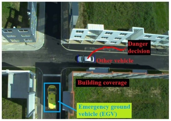
:Forerunner UAV refers to an unmanned aerial vehicle equipped with a downward-looking camera flying in front of the advancing emergency ground vehicles (EGV) to notify the driver about the hidden dangers (e.g., other vehicles). A feasibility demonstration in an urban environment having a multicopter as the forerunner UAV and two cars as the emergency and dangerous ground vehicles was done in ZalaZONE Proving Ground, Hungary. After the description of system hardware and software components, test scenarios, object detection and tracking, the main contribution of the paper is the development and evaluation of encounter risk decision methods. First, the basic collision risk evaluation applied in the demonstration is summarized, then the detailed development of an improved method is presented. It starts with the comparison of different velocity and acceleration estimation methods. Then, vehicle motion prediction is conducted, considering estimated data and its uncertainty. The prediction time horizon is determined based on actual EGV speed and so braking time. If the predicted trajectories intersect, then the EGV driver is notified about the danger. Some special relations between EGV and the other vehicle are also handled. Tuning and comparison of basic and improved methods is done based on real data from the demonstration. The improved method can notify the driver longer, identify special relations between the vehicles and it is adaptive considering actual EGV speed and EGV braking characteristics; therefore, it is selected for future application.
1. Introduction
The forerunner UAV concept was introduced in [1,2], the former discussing the formulation of the concept and the latter introducing the final concept of the demonstration system. It refers to a camera-equipped UAV flying in front of and above emergency ground vehicles (EGVs) to notify the driver about hidden threats covered by buildings, vegetation or other vehicles. The project “Developing innovative automotive testing and analysis competencies in the West Hungary region based on the infrastructure of the Zalaegerszeg Automotive Test Track” GINOP-2.3.4-15-2020-00009 targets to make a feasibility study of the overall forerunner UAV concept applying extensive simulation studies and a smallscale feasibility demonstration on the Zalaegerszeg Automotive Test Track. The project lasts from July 2020 to March 2023 and the real-life feasibility demonstration of the whole system was presented in September 2022 [3]. The risk evaluation of ground vehicle collision with the forerunner UAV is the main focus of this article, giving only an overview of the whole system concept, object detection and tracking. The previous publications focused mainly on the system concept [1,2], the simulation components of the forerunner UAV software-in-the-loop (SIL) simulation [4] and the challenge of tracking the EGV flying in front of it on a pre-planned route which can suddenly change [5]. Here, the details of the onboard system installed on the EGV and the additional onboard system of the selected DJI M600 hexacopter test vehicle [6] are presented in Section 2 together with the details of the applied test scenarios. Then the software structure consisting of control, camera and detection modules is presented in Section 3. These are all new unpublished details of the forerunner UAV test setup. The main challenge of the forerunner concept is the capability to decide if an approaching ground vehicle endangers the own EGV by not stopping or by stopping too late. As the forerunner UAV applies a stabilized downward-looking camera to monitor the traffic situation first, the other vehicles should be detected in the camera image. It is good to detect also the own EGV as will be discussed later, but it is not mandatory for the proper functioning of the system.
Camera-based object detection using neural networks has been witnessing a revolutionary change in the field of computer vision. Many detection algorithms emerged that are now capable of both successfully localizing objects on an image and specifying the category to which the object belongs; however, the inference time, or the speed at which one input frame is processed, can be significant even on dedicated high-end hardware. State-of-the-art object detection methods can be categorized into two main types: one-stage and two-stage object detectors. In one-stage detectors, the localization and classification are combined into one step to achieve higher performance at the cost of accuracy. In twostage object detectors, the approximate object regions are proposed using deep features before these features are used for the classification as well as bounding box regression for the object candidates. These methods achieve higher accuracy but are usually more resource-intensive than one-stage detectors. As the object detection must run real-time on the UAV, certain hardware limitations had to be considered, which narrowed down our object detector choices to one-stage detectors. The most popular one-stage detectors include Yolo, SSD [7] and RetinaNet [8]. Due to previous experiences with it, the final choice went to the Yolo (You Only Look Once) object detector. At the time of writing, the latest version was Yolov7 published in July 2022 [9], but due to better support and software compatibility, the predecessor Yolov4 [10] and Yolov5 [11] versions were only considered, of which Yolov5 proved to be slightly better both in detection accuracy and inference time. The detected objects then need to be tracked for the estimation of their trajectories.
Online Multiple Object Tracking (MOT) is often solved by data association between detections and tracks [12]. Data association can be seen as an optimization problem, where each pairing has its own cost. The two main components of the cost function are the motion model and the visual representation model of an object. Visual representation models make the tracking robust [13,14]; however, usage of these representations requires more computation. Each MOT solver needs to make a trade-off between speed and accuracy, especially on an edge computer. Neural networks dominate the field of object detection, and they are also capable of encoding visual representations during the detection step [15]. Simple online and real-time tracking SORT [16] is the baseline of MOT solvers with motion model, where the Hungarian algorithm provides the optimal pairing. Motion models are sensitive to camera movements, which are inevitable on a moving platform. One possibility to reach better tracking performance beyond using visual representations is 3D-reconstruction-based tracking, where the 3D object positions are estimated and tracked [17]. This approach can naturally handle occlusions and provide more robustness and scene understanding during tracking; however, it requires calibrated camera and accurate camera state estimation. MOT in this paper has some additional assumptions. The EGV sends its GNSS position to the drone, which helps the tracking of the EGV if it is in the camera image, and the GNSS altitude of the road is known. With these assumptions, the 3D trajectories of the detected vehicles can be tracked by a SORT-based method.
The training of the object detection methods is summarized in Section 4 while the details of object tracking are given in Section 5.
There is a broad set of literature about vehicle collision estimation considering different scenarios and approaches. Refs. [18,19,20,21] consider known position, velocity and even acceleration information while [22] considers images of a camera mounted on the own vehicle and [23] considers a large database about the road network and accidents. Ref. [23] applies machine learning methods to learn accident formation on the Montreal road network and, based on that, predict future accidents or dangerous road sections. Ref. [22] applies vehicle detection, lane detection and vehicle motion prediction mainly focusing on lane changes of the other vehicle considering the images from the viewpoint of the driver. Ref. [20] applies Long Short-Term Memory and Generative Adversarial Network to learn and predict vehicle trajectories on a longer, 12 to 20 min horizon based on 8 min of registered data.
Closest to our situation with known vehicle position are the works [18,19,21]. Ref. [18] considers rear end collisions and intersection accidents predicting close vehicle trajectories from position, velocity and acceleration data on a given time horizon. The prediction time horizon is varied and simulation evaluation considers driver response time and the time required to slow down the vehicle showing the cases when the driver notification is successful or not. Ref. [19] deals with rear end collision prevention in adverse weather conditions considering the effect of weather on driver reactions. It gives a good overview about the collision prediction methods including time to closest point of approach, stopping distance algorithm (SDA) and the machine-learning-based non parametric methods. In the solution of this paper, braking and reaction times of the driver are considered such as in [18]. Ref. [21] deals with deterministic prediction of vehicle trajectories based on simple Newtonian dynamics and the handling of uncertainties transformed from vehicle reference frame to North-East frame. A resulting normal distribution is applied to evaluate probability of the predicted vehicle positions, considering also vehicle size. Lane geometry is also applied to exclude positions outside the lanes. Finally, the method is verified in two simulated scenarios.
Considering the literature, the development goals in the forerunner project were to construct a parametric method for trajectory prediction and collision decision possibly also including the position uncertainties. The inclusion of EGV stopping time makes the trajectory prediction adaptive. Non-parametric methods are excluded because of the usually higher computational needs of machine learning solutions. As the back-projection of camera vehicle positions give North-East (NE) coordinates, the system dynamics are considered in the North and East directions, thus avoiding complications caused by vehicle to NE and backward coordinate frame transformations (see [21]). In case of accurate estimation, the separate North and East accelerations should give the same results as vehicle longitudinal and lateral acceleration transformed to NE frame with vehicle orientation. Contrary to the literature sources, the verification of the methods is done with real test data starting from the captured image sequence and finally arriving to the decision about ground vehicle collision.
Newtonian dynamics-based parametric prediction methods require the estimation of vehicle speed and acceleration from the camera-based position information. Vehicle speed estimation based on fixed cameras is discussed in [24,25,26,27]; however, as the forerunner UAV moves with the EGV, the camera is also moving, so UAV-based vehicle speed estimation methods should be considered as presented in [28,29,30,31,32]. Refs. [28,30] apply ground control point-based calibration of the scene, which is not feasible with the forerunner UAV as it should operate without such constraints. Ref. [32] applies a special calibration procedure from the literature, which again requires a predefined scene. Ref. [29] considers assumed vehicle sizes to scale the picture; however, the large variety of vehicle sizes makes this approach risky. Ref. [31] mentions the concept of fixed flight altitude and then applies road lane information to improve accuracy. In the current work, known flying altitude and flat plane assumptions are applied as mentioned before. These are all valid considering the precision of relative barometric altitude measurement and the relief of ZalaZONE Smart City, which is flat. Camera-based calculations lead to uncertain North-East position information (see Section 5) of the vehicles, from which the velocity and acceleration can be estimated with different methods [33,34,35,36,37]. Detailed evaluation of these literature sources is presented in Section 6. After velocity and acceleration estimation, the prediction of vehicle trajectories is required and, based on the predictions, a decision about collision danger should be made.
For the September 2022 demonstration, a very simple parametric method with a heuristic decision logic considering the main characteristics of the encounters was developed due to the time constraints. The detailed tuning of the basic method, the exploration of further possibilities and proposal of a more complex method are the main topics of this article. In Section 6, the basic method is presented first, then the development steps and results of the more complex method are shown. Apart from decision about the collision, several special scenarios can also be detected with the suggested method such as other vehicles behind, in front of or moving in the same direction as the EGV. Section 7 presents the parameterized form of the basic and improved decision methods for parameter tuning. Then, Section 8 presents the tuning results for the two methods while Section 9 compares them based on real demonstration data. Finally, Section 10 concludes the paper.
2. System Hardware Structure and the Demonstration Scenarios
The entire Forerunner UAV concept relies on the cooperation of an aerial and a ground vehicle (EGV). To make the UAV able to follow the EGV autonomously, a common communication link has to be established between the two vehicles. Among many alternatives, 5 GHz WiFi was chosen to be the platform of the communication. Both the EGV and the drone had to be equipped with additional hardware packages. Our goal was to make these hardware stacks as system-independent as possible. This was completely satisfied regarding the ground unit, since it can be mounted on top of any commercial vehicle; no additional components are required by the EGV to make the system work. Easy portability was very useful when testing, since the system was mounted on numerous vehicles, including an actual ambulance car (see Figure 1). On the other hand, the aerial hardware system can only be used on DJI M600 hexacopters, since both the mechanical and software architectures rely on the specifications of the aforementioned drone. However, with minimal design changes, it can be mounted onto other drones as well. Figure 1 and Figure 2 show the DJI M600 with the onboard system.
2.1. EGV Onboard Unit
The onboard unit installed on the EGV consists of a high performance MikroTik outdoor WiFi access point (WiFi AP), a custom designed RTK capable GNSS receiver (manufactured in Institute for Computer Science and Control (SZTAKI)), a National Instruments CAN-USB interface and a four cell LiPo battery to power them. A laptop is also necessary for collecting and sending the measurement data coming from the GNSS sensor. The block scheme and a photo of the actual hardware can be seen in Figure 3 and Figure 4, respectively. The hardware mounted on an ambulance car is shown in Figure 1.
The main task of the EGV onboard unit is to measure the position and velocity and send it to the drone. The measurement is carried out by the GNSS system, which supports RTK correction, and thus can provide centimeter precision position data. Besides position, the receiver sends velocity and timestamp values which are utilized as well. The actual hardware (hardware #2 in Figure 4) is designed by SZTAKI and was further developed and tested within the scope of the Forerunner UAV project. As it can be seen in Figure 3, the dataset is transmitted via CAN to a NI CAN-USB interface, which is connected to the laptop which receives and packs the valuable information. This is then transmitted to the drone’s onboard stack via the WiFi router. To ensure faster packet sending, the laptop is connected to the router with an Ethernet cable. The gray area in Figure 3 incorporates the devices present in Figure 4.
2.2. Aerial Vehicle Onboard Unit
Compared to the ground unit, the aerial onboard system has a few more components, as depicted in Figure 5 and Figure 6. As visible in Figure 5, the whole system relies on the DJI M600 platform because it provides power and data also to the payload. There are several sensors applied, including the same RTK GNSS sensor featured in the ground unit and a Basler industrial camera with an additional gimbal stabilizer. The core of the drone’s onboard system is the Nvidia Jetson Xavier NX single-board computer which is developed specifically for embedded applications focused on image processing. The Xavier NX features a 6-core ARMv8 CPU, a 384-core Nvidia GPU and 16 GBs of memory. It is connected to the DJI M600 via UART to receive measurement data from the drone’s onboard sensors and to send control commands. Moreover, the Basler camera is connected to it via Ethernet for image input. Orientation data is provided by the gimbal via UART to adjust the images created by the camera. Similarly as in the ground system the onboard RTK GNSS hardware provides accurate position data to the Xavier NX with a USB connection. Apart from that, the GNSS provides a trigger signal to both Xavier NX and the Basler camera. This signal causes the camera to take images and triggers communication between two processes running on the Nvidia computer. To receive information about the EGV’s location, the Xavier NX is connected to its WiFi AP. To provide more reliable network connection, the WiFi antennas of the Nvidia computer were upgraded from the factory ones, as shown in Figure 6.
As shown in Figure 5, there is a separate LiPo battery installed on the drone to power the gimbal. There is one usable UART port on the Xavier NX which is utilized for the connection with the M600, the other UART connection with the gimbal is implemented with the help of a USB-UART converter. Moreover, the ethernet connection with the camera is established with the built-in network socket on the Xavier NX. The trigger signal depicted in Figure 5 is a wiring between one of the GNSS’s pulse generation pins to one of the Nvidia computer’s GPIO pins. This is used to trigger communication between two software running on the computer. This is going to be detailed in Section 3.
2.3. The Demonstration Scenarios
The feasibility demonstrations were planned and presented in the Smart City module of ZalaZONE Proving Ground, Hungary [38]. Figure 7 shows the overall map of the ZalaZONE Proving Ground, highlighting the part of the Smart City module applied for the demonstrations and showing also an aerial photo of the intersection.
The intersection with the approaching vehicles is shown in Figure 8. The EGV always comes from the STOP sign, but it has the right of way, assuming it applies its sirens. The other vehicle comes from the right and three encounters are considered. First, it slows down and stops in time. Second, it comes fast and stops at the last possible moment. Third, it does not stop. As the walls cover the other vehicle from the EGV, the maneuvers were coordinated through radio communication, and in the third case, the EGV driver knew that he has to stop. The goal of these three scenarios is to test if the stopping attempt of the other vehicle can be detected or only ’other vehicle present / not present’ decisions can be done. Due to the dynamic limitations of DJI M600 (see [4]), the maximum speed of the maneuvers was 20–25 km/h. Higher-speed maneuvers will be evaluated in the SIL simulation ([4]) of the system. After the introduction of the hardware system and the demonstration scenarios, the software system is summarized in the next section.
3. System Software Structure
Apart from the appropriate hardware system, a suitable software set had to be developed in order to test the Forerunner UAV concept. The majority of development took place on the Xavier NX computer installed on the DJI M600, but there were also gimbal, RTK GNSS and ground laptop software developments. An overview of the software architecture and data flow can be seen in Figure 9. Highlighted in blue, there are three essential processes running on the Xavier NX. The first one is the control software, the second one is responsible for gathering camera images, multi-object tracking and decision (camera software), and the third one handles object detection (detect software). Each of them is detailed in the following subsections.
3.1. Control Software
Initial developments within the scope of the Forerunner UAV project were started by establishing communication between the DJI A3 flight control system present on the DJI M600 and the Xavier NX onboard computer. DJI’s M600 drone supports the Onboard Software Development Kit (OSDK) [39] provided by the manufacturer, which makes it possible for developers to interface with the drone via a UART channel. After a successful connection, various flight data can be obtained, like position, orientation and velocity. Moreover, reference commands can also be sent to the drone, which makes the developer able to control the drone from an external hardware. For the input of the control algorithm the Xavier NX receives position, velocity, acceleration and orientation (M600 Pose in Figure 9) of the drone in every control cycle which runs at 50 Hz. The control command consists of horizontal speed reference, altitude and yaw angle.
Another essential input for the control software is the data coming from the EGV. As described in Section 2, these packets are sent via WiFi using UDP protocol by the laptop of the ground unit. Each packet contains the EGV’s current high precision (RTK) position, velocity and timestamp. Figure 9 also shows EGV waypoints (WP) sent by the ground vehicle. They exist in the communication; however, the actual waypoint values were predefined in the control software as the ZalaZONE Smart City test track route was fixed in all tests. Still, the communication method supports a larger database of waypoints present on the ground unit. Apart from the messages coming from the EGV, the control software can read custom defined messages coming from the network. For example, there is a message defined to trigger the start of autonomous control, or to turn the gimbal on or off.
As shown in Figure 9, gimbal data is sent to the control software as well. Gimbal data refers to the roll and pitch angle of the inertial measurement unit (IMU) attached to the vertical camera on the gimbal. It is not utilized by the control software, only sent forward to the camera software alongside with the data received from the M600 drone. On the other hand, the connection with the gimbal can be used to tune the PID motor controllers. This was carried out manually with a trial-and-error method. The system had instability unless the camera was mounted on it, so tuning was successful only when the payload was attached. The tuning had to be carried out only once, since the camera mounting was not modified between experiments and the parameters of the gimbal proved to be stable (no changes with temperature).
Another important part of the system is the trigger signal sent to Xavier NX and the Basler camera. The signal generated by the RTK GNSS unit has nanosecond precision and is used to trigger the camera to take pictures. Inside the control software running on Xavier NX, this also triggers the communication between the camera and the control software. The messaging between the two is handled by UNIX domain sockets supported by the Ubuntu operating system of the Xavier NX. Apart from the trigger signal, the RTK GNSS provides high precision position of the DJI M600 to the control software. Therefore, it has two options to rely on when taking the own position into account. A simple logic decides whether the position information estimated by the A3 autopilot or provided by the custom RTK GNSS unit has to be used. This logic considers the A3 autopilot’s estimate to be the default, and if the RTK GNSS position is valid (close to the position estimated by A3), then that is forwarded to the control algorithm.
3.2. Camera Software
Aerial onboard computing systems require the separation of crucial control processes from mission payload computation. The A3 control unit of the DJI M600 platform provides the basic control and safety; however, it is still beneficial to separate the high level control from the image processing and the analysis of the traffic situations. High level control of the UAV is based only on the state of the EGV beyond its own state, while the output of the image processing and decision on traffic situation is an input for the human driver of the EGV.
Camera software (Figure 9) consists of the image acquisition, communication between the control and the object detection software components, and the tracking and analysis of the trajectories corresponding to each ground vehicle nearby. The component also sends a downsampled image processing result and the decision signal (possible danger) to the EGV through WiFi. For the above tasks, the camera software requires the state of the UAV along with the state of the EGV, the planned waypoints (intersections) and camera images with the corresponding gimbal state. The onboard camera [40] is a calibrated downward-looking 2048 × 1536 RGB camera with optics covering a 82-degree horizontal field of view (FOV). The relative altitude above the surface is known and the area is considered a horizontal plane. These assumptions are true at the test site, and with elevation map information, the calculations can be generalized by assuming a planar surface for each local region with known normal vectors.
For each hardware trigger, the camera produces an image (@10 Hz), which is saved as raw Bayer pattern to a binary file, and a downsampled version (1024 × 768) is passed to the object detection neural network (NN) as a shared memory file. The higher original resolution images can be used in later developments. The NN sends back the bounding boxes of detections with the class labels. The detections are projected to the North-East-Down (NED) coordinate system using the assumption of horizontal flat ground and known ground relative altitude, and tracking is done in the NED coordinate space (see Section 5). Risk evaluation is done for each track (see Section 6) and results are finally visualized in a 640 × 480 image with back-projections of the object NED coordinates. The danger signal and the resulting image are communicated to the driver of the EGV (see the Supplementary Videos).
3.3. Detect Software
The separation of the Yolov5s [41] object detection network from the image processing component was important to have more flexibility in the selection of the object detection method. This way, the complex inference engine is not compiled together with other parts of the image processing, and can be replaced easier. Furthermore, the NN part can use its python interface. Details about the selection and training of the object detection NN are provided in the next section.
3.4. Speed of Onboard Operation
Proper timestamping of sensory data is a key development parameter; thus, fixed FPS operation was considered with hardware trigger which was directly derived from the PPS signal of the GPS. Ten FPS was selected, because the average complete cycle of operation was 12 FPS with a minimum always above 10 FPS. One cycle of onboard operation consists of the image capture by the Basler camera driver and c++ API with SSD recording (in a separate thread), the downsampling of image and shared memory transfer to the python detection software, the inference of the object detection neural network, the transfer of detection bounding boxes and classes, the multi-object tracking and finally the decision on danger for each track. Beyond the detection and decision cycles, the control software also utilizes onboard computational resources, but the bottleneck is the shared memory map to the decision cycle.
4. Training of Object Detection
For object detection, due to the hardware restrictions of the Nvidia Jetson Xavier NX platform, the Python version of smallest Yolov5 neural network, Yolov5s, was chosen as object detector. In [4], Yolov3s and Yolov4s neural networks were compared to each other. The comparison showed Yolov3s to be slightly faster but less accurate than the Yolov4s version. The Yolov5s network was trained later, achieved similar results compared to the Yolov4s version (overall [email protected] of 0.878 compared to Yolov4s’s 0.876) but proved to be faster with an average inference speed of 22 FPS (compared to Yolov4s’s 12 FPS). Thus, finally, the Yolov5s was applied onboard the forerunner system.
Two separate neural networks were trained for the demonstration: one for testing purposes trained with simulated data from the driving simulator CARLA [42], and one with publicly available real-life birds eye view images of cars based on [43]. An average inference speed of 22 FPS was achieved using these networks on the Nvidia Jetson NX platform.
The CARLA database consisted of 2000 images with their respective bounding-box location (obtained from CARLA in the SIL simulation [4]). This network was trained for 3 classes—cars, bicycles and pedestrians—with a train/test split of 70/30 on 400 epochs with a batch size of 16. Training results can be seen in Table 1. From the high Precision value for all 3 classes, it can be seen that the network reliably classifies an object if it was detected, but, based on the Recall values, has problems with finding small objects on the images, especially pedestrians. Considering that pedestrians are only 1 or 2 pixels in size, this was an acceptable result for the smallest Yolov5 network.
The Yolo_RL real-life database was a combination of images from the PUCPR+ and CARPK datasets [44], amounting to 3000 images with around 100,000 cars recorded from different parking lots by drones at approximately 40 m height. Other datasets were considered as well, e.g., Vedai [45,46] and COWC [47,48] datasets, but these images either had low resolution or were taken from much higher altitude (ZalaZONE flight altitude was set to 40 m). The real-life Yolo_RL network was trained with 1 class only, cars, with the same parameters as the CARLA network. Training results for this network can be seen in Table 2. The high Precision and Recall values show that the network managed to learn the significant features of the cars contained in the Yolo_RL database.
Both trained networks showed good inference results in general, but after the first real-life test, it was apparent that the Yolo_RL dataset had a few shortcomings. On one hand, the lighting conditions were too ideal in the dataset; it had vehicles either in full sunlight or fully shaded and the network was struggling with situations when the vehicle was entering or exiting a shaded area. The other significant issue was the lack of road markings, such as STOP and priority indications where the network would either completely fail to detect the vehicle or would detect one vehicle as multiple ones (see Figure 10).
To eliminate these issues, the dataset was expanded with 1200 extra images containing such situations recorded with the DJI M600 on the ZalaZONE Smart City test track. The images were then labeled with Roboflow’s [49] annotation tool and then Yolo’s transfer learning function was used to fine tune the previous weights. With the fine tuning, these outlying cases were eliminated. A comparison of the inferences on the Yolo_RL network and the fine tuned network can be seen in Figure 10. After object detection, the next section summarizes the object tracking solution.
5. Object Tracking in the Demonstrations
The object tracking approach is a variant of the SORT [16] solver. In the case of online fast object tracking from frame to frame with a reliable detector these solvers utilize that the object positions are closer to a prediction from a linear motion model than the size of the object, thus intersection-over-union (IOU) is an effective indicator for data association. The reliability of these IOU-based metrics are improving with increased frames per second (FPS) and proved to be effective in tracking cars in an intersection [50].
SORT consists of a linear velocity predictor which is filtered by a Kalman filter considering detection uncertainties. The problem of optimal pairing is solved by the Hungarian algorithm based on the IOU cost of a pair. The main goal of tracking is to have an accurate series of center points for the detected bounding boxes. Detection inaccuracies may come from partial occlusions and small vibrations of the bounding boxes around the true value. As we have birds-eye-view images from the downward-looking camera, the center point of vehicles are stable without oriented bounding boxes. The UAV is a moving platform and other objects are also moving; thus, we did prediction and IOU calculations in the North-East-Down (NED) coordinate system (with fixed origin during the whole flight as the covered Smart City area is small). The detections in the image have nonlinear behavior, which can be eliminated by the transformation of detections to 3D (NED system) by utilizing relatively accurate UAV and gimbal states.
5.1. Projection of Bounding Box Centers to North-East-Down Coordinates
As the altitude of the ground surface is known, the Down (D) coordinate is also known; thus, we need to obtain North (N) and East (E) coordinates. First, undistortion is done on the image coordinates and based on a radial distortion model, which is available through camera calibration [51]. Let and be the coordinates of the principal point and , be the 2nd and 4th order distortion coefficients. The square of the normalized distance from center () is given in (1), where and are the focal lengths in pixel.
With , the undistortion fraction of the coordinates can be calculated as (2). The undistorted pixel coordinates are and .
With the undistorted coordinates, let denote the normalized vector pointing towards the undistorted pixel from pinhole origin. We need the coordinates of this vector in Earth NED coordinate system . With the camera to gimbal axis, swap matrix (4) and gimbal to Earth NED transformation matrices . The Earth NED coordinates of the UAV and relative position of the camera on the UAV are known; thus, Earth coordinates of the camera are also known (see (6)). At this point, the intersection of the line starting from with direction vector and the horizontal plane at down position D can be determined as (3), giving the North-East-Down position of the object.
of (4) is a necessary axis swap matrix when one changes from image xy and depth z coordinates to the gimbal system.
gimbal to Earth transformation can be formulated from gimbal pitch and roll Euler angles (,) together with UAV yaw angle ():
Let denote the NED coordinates of the UAV and the relative position of camera to the center of the UAV (in body system). can be obtained considering UAV Body to Earth transformation from UAV Euler angles (yaw , pitch , roll ):
5.2. EGV Tracking and Management of Other Tracks
EGV tracking can be done using the RTK GNSS data coming from it; however, the EGV is in the image most of the time, and the RTK NED data can be projected back to the image plane which indicates if a detection in the image is the EGV. Beyond the simple pairing of EGV detection, it provides a system integrity check opportunity if the EGV is present in the image. The only drawback is RTK state frequency (5 Hz), which can be enhanced by a Kalman-filter-based sensor fusion on the ground navigation unit.
After the pairing of the EGV detection (if it exists), the rest of the detections are paired to existing tracks with SORT, where a filter on maximum speed is applied. Unmatched detections are considered as new tracks, and a track after 5 consecutive steps without a match is dropped.
The next section summarizes the risk evaluation methods starting with the basic one applied in the fall 2022 demonstration [3] and then presenting the detailed development of a more complex method.
6. Risk Evaluation in the Encounters
After detecting and tracking the vehicles (EGV and other) in the NED system, their velocity and acceleration should be estimated to predict their future movement with Newtonian dynamics similarly to [21] and decide about the collision risk. In the feasibility demonstration in September 2022 [3], a simple prediction and decision method was applied due to the lack of development time. However, all image sequences and DJI M600 onboard and EGV log files are saved so offline processing and algorithm development is possible. After summarizing the basic prediction and decision method in Section 6.1, detailed analysis of the data and development of an improved prediction and decision method are presented in Section 6.2.
6.1. Basic Decision in the Feasibility Demonstration (September 2022)
Due to the time constraint in preparation for the demonstration a very simple position prediction and risk evaluation method was developed. The basis is a windowing technique both for the back-projected North (N) and East (E) positions applying window size. First, the norm of the position displacement in the window is calculated as . If , the estimated velocities are zero and the estimated positions are the means of the last three values , . If , the estimated positions are the last measured ones and the velocities are estimated by fitting a line to the points in the window and taking the slope as velocity ().
Prediction of vehicle motion is done on a 1.5 s horizon having 20 equidistant points with time values. In case , the predicted position is , where M represents either N or E. In the other case, . This is similar to the stopping distance algorithm mentioned in [19] and the deterministic prediction in [21] but without the consideration of acceleration.
Risk evaluation is done by calculating the distances of the predicted positions and comparing them to an adaptive threshold: where heuristically tuned and calculated from the estimated vehicle velocities. This way larger THS is applied in case of larger vehicle velocity. If the distance is below the threshold then there is a danger of collision and the EGV driver should be notified.
The initial parameters () were tuned by trial and error considering pre-collected real flight data from ZalaZONE SmartCity. Detailed parameter tuning is presented in Section 8.
6.2. Improvements in the Decision Method
As described in Section 3 synchronized camera image, onboard DJI and EGV data are continuously logged with 10 Hz frequency (giving also 10 FPS camera information). Thus, besides the camera images, gimbal angles, drone position, velocity and orientation, the EGV position and velocity are all available in a synchronized manner. For higher EGV speeds, this limitation to 10 FPS can possibly degrade encounter risk evaluation performance but this will be the topic of the planned detailed feasibility study. Unfortunately, during the demonstration flights, the RTK GNSS system onboard the M600 had a connection problem (caused by a loose connector), which is why only the normal GNSS-based data from the DJI M600 A3 autopilot was available with lower (few meters) precision. It is the output of a GNSS-IMU fusion algorithm. The NED position of the detected objects is calculated based on this position information thus it is inaccurate compared to the RTK GNSS position of the EGV. As both the EGV and other vehicle positions are back-projected to the NED system (see Section 5), this causes a larger difference between logged RTK GNSS EGV track and the back-projected one, as shown in Figure 11 and Figure 12.
There is not only a side error but also an error along the track between the RTK and projected data (see Figure 12). This could be because of wrong synchronization, but analysis of several tracks has shown that this error is caused by GNSS positioning uncertainty. Considering this, it is better to process the back-projected EGV and other vehicle tracks instead of processing the EGV RTK track and the back-projected other vehicle track. In the former case, the two tracks have similar systematic errors which can increase decision accuracy while losing the advantage of accurate logged EGV position and velocity data. New experiments are planned in Spring 2023 with updated onboard RTK GNSS hardware to have more accurate DJI M600 position. However, the current measured RTK GNSS EGV position and velocity values provide a possibility to satisfactorily evaluate the precision of the velocity and acceleration estimation methods based on the back-projected positions. Hence, first, EGV velocity and acceleration estimation is developed in Section 6.2.1, Section 6.2.2 and Section 6.2.3, evaluating accuracy based on the RTK GNSS position and velocity measurements. Then, motion prediction and risk evaluation are discussed in Section 6.2.4 based on the selected best velocity and acceleration estimation method.
Before starting to develop EGV velocity and acceleration estimation methods, the RTK GNSS and back-projected EGV North-East positions are plotted in Figure 13 to be able to compare them. The figure shows that while 10Hz sampled back-projected EGV positions are continuously changing and uncertain, the RTK GNSS position is quantized due to its only 5 Hz sampling. This can later be resolved by predicting positions from the RTK GNSS velocity measurements between the samples. Looking for literature sources about the topic of position measurement-based velocity and acceleration calculation mostly electric motor related sources can be found considering encoder measurement of angular position and estimation of rotational speed and acceleration [33,34,35,36,37]. As the mathematical principles are the same, these methods can well be applied for the forerunner UAV.
Ref. [33] introduces the fixed time (encoder distance in a given time) and fixed position (time to cover a given distance) methods considering first order difference, Taylor Series Expansion, Backward Difference Expansion and Least Squares Fit calculations. The last means fitting a smoothing polynomial to the measured position data and then the first derivative gives the velocity while the second gives the acceleration.
Ref. [34] also applies polynomial fit on a moving window and gives a tuning method for a required precision.
Ref. [35] introduces the so-called encoder event (EE) for quantized data, taking the mean of measured values and time stamps when the measured signal changes. This is illustrated in Figure 14 with and . Then, it applies polynomial fit to pairs and interpolates the original time values.
Ref. [36] introduces the Single-dimensional Kalman filter (SDKF) concept, applying a one-dimensional KF (Kalman filter) to smooth the velocity considering an adaptive state noise covariance gain. A phase-locked loop (PLL) is applied for acceleration estimation.
Finally, Ref. [37] gives a good overview about the available methods listing finite difference and low-pass filtering, EE with finite difference and skipping option (neglecting some events to have a smoother curve), polynomial fitting, KF estimation including SDKF and finally sliding mode differentiators for velocity estimation. For acceleration estimation it considers EE with 2nd order finite difference and smoothing, position SDKF and 2nd order finite difference, sliding mode differentiators and control loop-based estimation with PD control or PLL. In the final comparison, Kalman filters with adaptive weights gave the best solutions both for velocity and acceleration.
6.2.1. First Order Differentiation
Pursuing the simplest solution and for the basic analysis of data first, simple differentiation of the measured North and East positions is done comparing the results to the measured RTK GNSS velocities. Figure 15 shows that though the trend of the estimated velocities is close to the RTK GNSS measured ones the result is too noisy even for vehicle motion prediction. This means that methods with data smoothing property should be applied. Note that, from now on, all velocity and acceleration estimation results are presented plotting the 80 to 110 s section of the first dataset to make comparison easier.
6.2.2. Filtering and Polynomial Fit
The next evaluated method was SDKF smoothing of position data (North and East) then polynomial fitting to estimate the velocity. From the estimated velocity, acceleration is estimated with a two-state (velocity and acceleration) adaptive measurement error covariance Kalman filter. This was selected because estimated velocity smoothing with SDKF and acceleration estimation based on polynomial fit gave unsatisfactory results.
As the RTK GNSS only gives position and velocity information, the acceleration should be estimated to be able to compare it with the back-projected position-based estimates. Because of the 5Hz sampling and high precision, the RTK GNSS velocity is quantized; hence, first, EEs should be collected as shown in Figure 14. After collecting the EEs, a moving window (tuned to have W = 4) technique is applied fitting lines to the EEs and having the slope of the line as the acceleration value at all time instants (overwriting some of these values in the next step). Figure 16 shows that the estimated acceleration is noise free and both the magnitude and the changes are in good agreement with the changes in the velocity. Thus, this estimate is proper for the evaluation of back-projected position-based estimates.
For SDKF smoothing, the covariance of the position measurement error is required and it can be estimated considering the back-projected EGV positions when the EGV is steady. Before every flight there is a section of the mission when the M600 positions itself above the EGV giving plenty of images with standing EGV (see Figure 1). Calculating the back-projection of these positions and excluding the outliers more than 5 m away from the mean the variance can be easily calculated after subtracting the mean position value. Table 3 shows the North and East variance results from four flight missions. The uncertainty of the values is high but taking the overall average can be a good approach.
The equations of SDKF (one dimensional KF) for position smoothing are presented in (7). Here, x is the state, which is either North or East position, P is the estimation error covariance matrix, Q is the state noise matrix (tuning parameter), K is the Kalman gain, is measurement noise covariance matrix and M is the measurement (again either North or East position). is a predicted while is a corrected value. Note that here both P and R are scalars, so the matrix inversion simplifies to division.
After tuning, the North and East SDKF were run with parameters and . Then, lines (first order polynomials) were fitted to the smoothed position data applying a size moving window to achieve further smoothing. The slope of the line is the estimated velocity at the last point of the window. was selected to have appropriate smoothing and minimum delay in the velocity estimates. An example result is shown in Figure 17.
The figure shows that the result is much more smoother than from simple numerical differentiation (see Figure 15) but it has noise. The trend of velocity estimates is similar to the RTK measurement with some larger differences at about 103 s in North and 92 s in East component. The difference of the North component can be checked in Figure 11, which shows that the back-projected North position is almost constant while the RTK position has the same slope as before.
Because of the high noise in the estimated velocity, instead of SDKF smoothing and line fit, a two state Kalman filter is implemented having the estimated velocity as measurement and velocity and acceleration as states. Its equations are presented in (8). Here, is the North or East velocity and acceleration state, is the state transition matrix with sampling time, is the state noise matrix considering only acceleration state noise with Q covariance, is the state measurement matrix, is the varying measurement error covariance matrix. Here, is the maximum velocity error from which the error variance can be obtained, considering it as the bound . is a scaling factor and, again, M is either North or East. is estimated as the absolute difference of velocity from first order differentiation and velocity from SDKF smoothing and line fit. This way, the measurement error covariance is adaptive. Tuning of the filter for minimum delay and maximum noise attenuation in acceleration resulted in , and both for North and East directions. Figure 18 shows the results compared to the RTK GNSS velocity-based acceleration. Though the trend of the RTK values is followed, there are very high peaks giving unrealistic accelerations. That is why some other estimation method should be found if possible.
6.2.3. Kalman Filtering Only
Considering [37] after the combination of filtering and polynomial fit, it is worth attempting the estimation of velocity and acceleration with one Kalman filter for each direction. An extra advantage of Kalman filter estimation is to have estimates of position, velocity and acceleration uncertainty from the estimation error covariances, as these are required for predicted position uncertainty estimation according to [21]. The filter equations are the same as (8) but now the state vector is , so position, velocity and acceleration (M is either N or E), , , having again only acceleration state noise.
The initialization of the filter is done from the first two position measurements having . At the first measurement, the state is simply .
was preserved from the SDKF and after tuning and resulted both for North and East directions. Tuning targets were minimum delay and maximum noise attenuation in velocity and acceleration. Results are shown in Figure 19, Figure 20 and Figure 21. Figure 19 shows the smoothing effect of the KF. Figure 20, compared to Figure 17, shows that the estimated velocity is smoother but has some larger differences from the RTK GNSS velocity. This is caused by some larger differences between the measured and estimated positions, as shown in Figure 19. Figure 21 shows that the acceleration is much smoother than in Figure 18 and its absolute maximum values are much smaller, being closer to the RTK GNSS-based accelerations. Finally, for the back-projected EGV North-East position data, the Kalman-filter-based estimation solution is the best as for the electric motor encoder measurements in [37].
An advantage of the three state KF is having an estimate of the variance of position, velocity and acceleration which can be utilized in the motion prediction as in [21]. While in the reference there is no given method for the estimation of these covariances, here they naturally result from the KF. Estimated standard deviations (STDs) are calculated by taking the diagonal of the estimation error covariance matrix P (considering only the variances) and then taking the square roots of the values. STDs are shown in Figure 22. The figure shows that the STD of position estimate is about 0.4 m, that of velocity is about m/s while that of acceleration is about 2.2 m/s2. The position is realistic; the velocity is a bit high giving a bound about 4 m/s, which is in the magnitude of the estimated velocities, and the acceleration uncertainty is very high compared to the maximum 4–4.5 m/s2 acceleration values (see Figure 21). This should be considered in the prediction and decision algorithm.
While the developments were done on the EGV trajectories, the tuned method will be applied on all detected vehicle trajectories assuming similar noise characteristics which should be true as the same M600 navigation data and camera parameters are applied for all objects. The next part discusses the motion prediction of the objects and the decision about the risk of collision.
6.2.4. Motion Prediction and Risk Evaluation
After estimating the position, velocity and acceleration of the vehicles, their future relative position and the risk of any collision should be determined. Note that while the tuning of the estimator was done on the whole trajectory of the EGV as it is always in camera FOV, for the risk evaluation the time synchronized EGV and other vehicle trajectories should be considered having short sections of trajectories when both vehicles are in camera FOV.
As the EGV driver can only react to dangers being in front of it or coming from the sides, objects behind the EGV should be filtered out as it is the responsibility of the driver approaching from behind to avoid collision. Thus, a half plane can be filtered out in every case considering EGV position and its direction of motion as shown in Figure 23. Defining as the unit vector pointing from object to EGV position the condition is where · defines the scalar product and is a unit vector. This is SC1 special case. In case and thus the object is ahead of the EGV, there are two more special cases:
- SC2: Object is in front of EGV, comes toward it (head on collision possibility) and so the driver should see it. meaning that the object and its moving direction is in range relative to EGV moving direction and the object comes towards the EGV.
- SC3: Object is in front of EGV, goes into the same direction and so the driver should see it. meaning that the object and its moving direction is in range relative to EGV moving direction and the object goes into the same direction.
These tests are only executed if the EGV absolute velocity is above 1 m/s. Considering that the building walls or other objects can narrow the driver’s field of view, the assumption should be refined later, but this is not the topic of this article. As the results show that no danger decision is masked because of this assumption, it is thus appropriate in the demonstration scenarios. Due to the estimation uncertainties, these special cases are declared only if the conditions are valid in 5 subsequent time steps (meaning about 0.5 s with 10 FPS). If they are declared, then no prediction of trajectories and decision about the risk should be executed.
The prediction of EGV and other vehicle trajectory can be done based on the estimated position (), velocity (), acceleration () and their STD values (). However, at the first two steps when the KF is initialized, only the measured positions and the estimated measurement uncertainty can be considered. Hence, the predicted position is with an uncertainty radius m. In the NE plane, the predicted NE positions (for EGV and other vehicle) give two points and the uncertainties can be considered as circles around these points. That is why is called the uncertainty radius. Finally, the intersection of the resulting two circles is tested. If they intersect, then there is a danger of collision.
The transient of the STDs after KF initialization is smooth (see Figure 24), so the future positions of EGV and other vehicle can be predicted without waiting for KF convergence. The prediction is done propagating velocity and acceleration into the North and East directions, considering also position and velocity uncertainty. Acceleration STD is too high to be considered if one wants to avoid overly conservative results. The equation for the predicted position including uncertainties thus results as (similarly to [21] having deterministic prediction with stochastic uncertainty):
This is similar to the stopping distance algorithm mentioned in [19] now considering also the accelerations and the same as the deterministic prediction in [21]. In the equation and is the prediction time horizon. Contrary to the previous steps, now the uncertainties are considered as the bounds instead of the ones again to prevent overly conservative results. In the previous steps, the bounds are reasonable because of the lack of detailed uncertainty information. Tuning of the sigma bounds will be presented in Section 8. (9) can be separated into deterministic prediction and uncertainty parts:
The equation shows that the uncertainty increases with the prediction horizon, which is a valid result according to [21] where the change with time is mentioned but no exact relation is provided. In case of different velocity and acceleration signs it is assumed that the vehicle decelerates only until stop and so the prediction time is limited to in each direction.
The maximum prediction horizon should be determined considering the EGV braking characteristics as the driver should be warned in time (similar to [18,19]). Firm and emergency braking times of a car were collected in real experiments starting from different velocities. The maximum results are summarized in Table 4.
Simple line fits can well cover the results so the braking time calculation formulas from the vehicle velocity are:
Figure 25 shows the measured data and the line fits. Though, theoretically, the braking time from 0 m/s is zero, the lines were fit with nonzero initial values to better cover the data and have some safety tolerance.
Besides the braking times, the braking distances were also registered in the experiment having the possibility to fit second order polynomials (going through (0,0)) and obtain a braking distance D model:
The maximum EGV braking time is determined from its actual RTK GNSS measured velocity with (11) and it is divided into 5 equal sections to evaluate the risk of collision in five subsequent predicted positions. If the uncertainty circles intersect each other, then a collision warning is activated. Any small intersection is considered dangerous as only bounds are considered in the uncertainties and the acceleration uncertainty is neglected. A measure of circle overlapping, tuning of its threshold and tuning of the sigma bounds will be presented in Section 8. Another important fact is that the predicted trajectories only cover the motion of vehicle center points so vehicle sizes should also be considered (see [18] for the precise definition of collision considering vehicle size and the consideration of vehicle size in the occupancy grid in [21]). Vehicle sizes are not explicitly handled here as this requires also vehicle size estimation from the bounding boxes. Instead, even tangent uncertainty circles are considered as collision (other cases are detailed in the tuning of the algorithm see Section 8). In case of unsatisfactory results, detailed consideration of vehicle sizes should be implemented. As there can be outliers, notification of the driver is only done after two consecutive warnings and the notification is stopped after ten consecutive safe evaluations. If any special case is decided, no risk evaluation is done until the special case is valid. The next section presents the parameterized basic and improved decision methods for parameter tuning.
7. Parameterized Basic and Improved Decision Methods for Tuning
For the detailed tuning of the methods, the parameters affecting the outcome of the decision should be selected and their realistic ranges determined.
7.1. Parameterized Basic Decision Method
The first variable parameter is the calculation window size W. As line fitting is done (requiring at least two points) its minimum value should be 3 to smooth the data. The maximum value was selected to be 9 having difference from the originally applied value. Accordingly . If the estimated velocities are zero and the estimated positions are the means of the last three values , . If the estimated positions are the last measured ones and the velocities are estimated by fitting a line to the points.
The prediction time is the next value affecting the decision. Its range was selected between 1 s to 2.5 s with s steps. As the reaction time of the driver can be considered as 0.6–0.7 s, 1 s prediction is the minimum to notify the driver. The s value was selected considering the fact that the object is maximum 3.5–4 s long in camera FOV (this was evaluated separately and is not in the scope of this work) and s is the time of firm braking from 30–40 km/h (see Figure 25) well above the maximum 1.8–2 s braking time from the 20–25 km/h speed of the experiments. This means that s maximum prediction time should be enough in this velocity range.
Risk evaluation is done by calculating the distances of the predicted positions and evaluating them against an adaptive threshold. The parameters of threshold calculation are the further tuning parameters: where . The distance was considered in the range 2–6 m with steps 2 m (±2 m from the original value) and the velocity scale was considered in the range 2–8 again with steps 2 (original was 6). Table 5 summarizes the parameter notations and ranges.
7.2. Parameterized Improved Decision Method
In this method, the main tuning parameters are prediction time and multipliers of position and velocity uncertainty in the uncertainty radius. The latter can be modeled as: where and is the prediction time horizon. The multipliers ( are considered to be as this covers of the possible estimated parameter range (assuming Gaussian distribution).
The prediction time horizon is determined by the braking time of the EGV from the actual speed as shown in Figure 25. This can be varied by shifting it forward or backward in time. The modified braking time equations result as: . is considered in the range s with s steps.
Another variable parameter is the overlap between the circles. At first, tangent circles were considered to give danger of collision but this condition can be relaxed considering circle overlap. The best solution would be a measure proportional to the overlapped area but its calculation is complicated so a simplified measure can be derived from the ratio of circle center distance and the sum of radii as Figure 26 and (13) show. Here, is circle center distance and and are object and EGV predicted position uncertainty radii, respectively. The resulting measure is 0 for tangent circles and 1 if the circle centers coincide. Starting from the tangent circles, the threshold () for circle overlap decision is considered between 0 and with steps. More than 50% overlap is possibly too large for proper decisions and this will be verified by the test results later (see Table 10). If is above the than a danger of collision is considered.
As both the decisions and the evaluation of the decisions (see the next subsection) apply the firm and emergency braking distances, their combination can also be a tuning parameter. Table 6 shows the considered combinations and their notations. When deciding based on firm braking time, firm or emergency braking of the driver can be considered in the evaluation leading to and combinations. When deciding based on emergency braking time, there is no point in considering firm braking of the driver as it will surely lead to collision, so only combination should be considered.
Finally, the tuning parameters for the improved decision and their ranges are shown in Table 7.
7.3. Evaluation of the Situation after Decision
Both the basic and the improved decisions were evaluated considering the time when the driver is first notified about the danger. From this time, the reaction time of the driver is considered to be s and the braking distance of the EGV (from the current velocity in (12)) should be considered. Considering also the current position and the estimated motion direction (from estimated velocity) of the EGV, the predicted stopped position can be calculated as:
where is either or depending on the case. This way the distance of the EGV’s stopped position from the track of the other vehicle should be evaluated to find the minimum. However, first, the relation of the EGV’s stopped position to the track of the other vehicle should be evaluated as shown in Figure 27.
The figure shows that the EGV can either stop before () or after () the track of the other vehicle, the latter case having the danger of collision. Therefore, before calculating the minimum distance, safe or dangerous stop position should be decided. In the safe case (), the distance is smaller than any distances between the current EGV position and the points of the object track. In this case, the calculated minimum distance (between and the other vehicle track) obtains a positive sign, while in the dangerous case ( with larger than at least for a few i) it obtains a negative one.
Another evaluation criteria is the longest time until the system shows danger to the driver after a first decision , hereafter referred to as danger notification time (DNT). This is an important parameter as too short notification of the driver has the risk of disappearing signal before the driver observes it and reacts accordingly. However, a danger notification cannot be held for a long time as, on a longer time horizon, new encounters and therefore new dangers can appear.
8. Parameter Tuning of the Methods
Flight data from four demonstration flights at ZalaZONE Proving Ground was collected considering three encounters per flight as described in Section 2.3:
- 1st encounter: The other vehicle comes slowly from the right and stops well in time. This should be classified safe by the system.
- 2nd encounter: The other vehicle comes faster from the right and stops with emergency braking. This should be classified safe.
- 3rd encounter: The other vehicle comes fast from the right and does not stop; the EGV should stop. This should be classified dangerous.
Here, Matlab calculation results are presented based on the recorded data but off-line processing of recorded data with running the flight codes on the same Xavier NX hardware is also possible with DJI M600 standing on the ground. The Supplementary Videos are generated this way. Tuning of both methods was done considering all parameter combinations for all flights and encounters. The detailed parameter tuning results are included in the Supplementary Files Parameter tuning basic method.xlsx and Parameter tuning improved method.xlsx; for details, see the description in the Supplementary Materials.
8.1. Tuning Results for The Basic Decision Method
Encounter evaluation was run for all parameter combinations from Table 5 and all flights. In the evaluation of the results, only the first two flights were considered as the trajectories of the other vehicle are too short in flights 3 and 4, missing the time slot when the other vehicle crosses the moving direction of the EGV (unfortunately, there is a gap in other vehicle tracking). This is shown in Figure 28 and Figure 29.
The evaluation for flights 1 and 2 was done considering the important decision requirements listed below:
- Decide safe situation for 1st encounter.
- Decide dangerous situation for 3rd encounter.
- Give a safe stopping distance at least with emergency braking for the 3rd encounter.
Coloring rules for the supplementary table Parameter tuning basic method.xlsx were generated according to this (see the Supplementary Materials).
For flight 1 the parameter sets satisfying the above rules were as shown in Table 8.
Comparing this parameter set with the valid flight 2 parameter sets gave only one valid parameter combination making the selection very simple. The selected parameters are:
The detailed evaluation of all flights for this parameter set is presented in the next section.
8.2. Tuning Results for the Improved Decision Method
In this case again the results for flights 1 and 2 were analyzed considering the FE combination as the most realistic candidate method. This means decision about the danger based on the firm braking characteristics but evaluation assuming emergency braking of the driver possibly giving the largest minimum distance between the vehicles. The tuning results in Parameter tuning improved method.xlsx show that the largest minimum distances result for , which is not surprising as danger detection will be the earliest considering even the tangent circles overlapping. As the resulting minimum distances are not too large, is fixed in the future evaluation. is also fixed to consider exactly the given braking characteristics. Later, presenting Tables 10 and 11 all related effects will be analyzed in detail. The main rules from the previous part were preserved, so first, the 3rd and 1st encounters are evaluated collecting the parameters valid for both of them. Table 9 first lists the valid sets in the 3rd encounter of flight 2 as this is the most critical giving the least valid combinations (see the Parameter tuning improved method.xlsx Supplementary Table). The later encounters and flights are compared to these sets. The table shows that all selected six parameter combinations give satisfactory results for the 3rd encounters but in the 1st encounter of flight 1 only and are good. In the 1st encounter of flight 2, the vehicles are too close to each other, so none of the combinations give valid results and danger is decided with all of the parameter combinations (see Tables 13 and 15 for the detailed evaluation). Considering the DNT, finally the combination is selected with , , .
After selecting the best parameter set, its evaluation against other parameters and cases should be done. Table 10 shows the effects of threshold change when . The table shows that, contrary to the overall observation in this case, there is no significant effect having the same minimum distances and DNTs in three cases. Further increasing the threshold causes a decrease in both distance and time as expected as higher overlap of the uncertainty circles will only appear in a closer position of the vehicles. The distance and time values in the last two cases show that there is no overlap above the measure during the encounter (there is no danger notification). This verifies the selection of as the maximum measure.
Table 11 shows the effect of time shift of the braking time with fixed value on the same parameter set. The table shows that the selected parameter combination has some ’robustness’, giving acceptable minimum distance even with 0.2 s less braking time. This time means shorter prediction horizon and so the danger decision is done later. This is shown by the decreasing DNTs () and the usually decreasing minimum distances by decreasing the time shift value. This analysis shows that this parameter set can also be valid for other vehicles with shorter or longer firm braking times and so prediction horizons.
9. Detailed Evaluation with the Selected Parameters
After tuning the methods, a detailed comparison of their performance should be done. The selected parameters of the basic method are:
while for the improved method the selected parameters are (with firm-braking-based decision and emergency-braking-based evaluation):
This section will first evaluate the results through tabular data with the selected parameter sets for basic and improved decision. The tables show the most important properties of the algorithms such as the expected and obtained decision (safe (S) or danger (D)), the minimum distance between predicted stopped EGV position and the other vehicle and the driver notification time (DNT). Another useful parameter is the measured minimum distance between the trajectories. Then the second part of the section will give deeper insight plotting relevant encounters and explaining them.
The decision results of the different encounters with the selected parameter set of the basic method are presented in Table 12. The table shows that with the selected parameter set the 1st encounter is always decided to be safe as expected. However, the 2nd encounter is always decided to be dangerous while the 3rd encounter is once falsely identified to be safe. Note that this encounter (flight 4/3rd) was not included in the selection of the parameters considering only flights 1 and 2. Three distance measures are presented in the table, the first (Real MIN. distance) being the minimum distance between EGV and other vehicle trajectories, the second (Firm MIN. distance) being the minimum distance between the stopped EGV (with firm braking) and the other vehicle, and the third (Emergency MIN. distance) being the same but with emergency braking. The smallest real minimum distance for the 1st encounters (all decided to be safe) is m so the 12 m for the 3rd encounter in flight 4 is reasonable to be decided as safe. As this flight case has a truncated track (see Figure 29) this can cause the larger distance and missed detection but this is a serious flaw of this selected parameter set. The safe or dangerous decision ’threshold’ (not a real threshold as the decision is based on other parameters) should be between m and 11 m as the latter is decided to be dangerous for the 3rd encounter of flight 3. For the 2nd encounters, the real minimum distances are between m and m, all being below 11 m, so it is again reasonable to decide them as dangerous situations. Considering the minimum distances between the stopped EGV and other the vehicle with firm braking they can be negative showing that the EGV passed the trajectory of the other vehicle. This happens only once for the 3rd encounter of flight 1 and is shown in Figure 38. The figure shows that, with firm braking, the EGV passes the trajectory, while, with emergency braking, it does not. This is underlined by the tabular data as emergency braking gives a positive minimum distance. Emergency braking usually gives larger distances as expected except for the 2nd encounter in flight 2. Figure 30 shows this encounter. The emergency and firm braking stopped positions are close to each other so the difference in the distances is not significant.
The table also shows that the DNT values are small, ranging from 0 s to 0.4 s. This is underlined by the colored danger notification sections of Figure 30.
The decision results of the different encounters with the selected parameter set of the improved method are presented in Table 13 considering firm braking both in the decision and evaluation. The table shows that with the selected parameter set the 1st encounter is once falsely identified to be dangerous while all 2nd and 3rd encounters are decided to be dangerous. Compared to the basic method this shows that here the real minimum distance ’threshold’ value (not a real threshold as the decision is based on other parameters) is shifted deciding danger even for 12 m distance. This corrects the false decision of the basic method for the 3rd encounter in flight 4. Here, the minimum distance limit for danger or safe decision is somewhere between 12 m and m, the latter is decided to be safe in the 1st encounter of flight 1. Regarding the minimum distances between EGV stopped with firm braking and the other vehicle (Evaluation MIN. distance), negative values result in three cases (twice for 2nd and once for 3rd encounter) showing stop after crossing the other vehicle’s trajectory. From these three cases, the 3rd encounter can cause problems as it is a collision situation. In the other cases, positive distances above 3 m are satisfactory. The DNT values are at least 1 s but they are above s in most of the cases being larger than the DNTs with the basic method.
The decision results of the different encounters with the selected parameter set of the improved method are presented in Table 14 considering emergency braking both in the decision and evaluation. The table shows that with the selected parameter set the 1st encounter is always decided to be safe while the 2nd and 3rd encounters produce uncertain results decided to be safe twice and dangerous also twice. This is too much uncertainty in the decisions so the emergency braking time criteria is not proper for decision. There is no point in evaluating the minimum distances and danger notification times this case.
The decision results of the different encounters with the selected parameter set of the improved method are presented in Table 15 considering firm braking for the decision and emergency braking for the evaluation. This is the test scenario applied for the selection of the parameters. The table shows that, with the selected parameter set, the 1st encounter is once falsely identified to be dangerous while the 2nd and 3rd encounters are always decided to be dangerous. Considering the real minimum distances again, if the 12 m distance for the 3rd encounter in flight 4 is considered to be dangerous (as expected), it is not surprising that the 1st encounter in flight 2 with m distance is classified to be dangerous. This is similar to the firm decision/firm evaluation (FF) case presented in Table 13. In this case, negative minimum distances between stopped EGV and other vehicle trajectory only appear twice for 2nd encounters, which is an improvement relative to the FF case where also a 3rd encounter produced negative distance. Considering the fact that the other vehicle stops before the intersection in the 2nd encounter, this can be considered a safe situation. Figure 31 shows that the predicted stopped positions appear with assumed forward moving direction of the EGV while its real motion is turning to the left. Considering the dense position sets of the other vehicle (showing its stopped position), the assumed moving direction of the EGV is surely far from it for flight 2. In case of flight 3, the assumed EGV track and stopped other vehicle position are close, possibly causing a dangerous situation if the EGV goes forward. Performance of the developed algorithm in such situations will be carefully examined in the future simulation test campaign considering much more situations than the encounters in the demonstrations. It is also worth noting that these demonstrations were somehow unrealistic because at least one of the vehicles had to stop in order to prevent accidents. In the simulation campaign, no such limitation will appear. In the 3rd encounters, the minimum distance is 1.46 m but the other values are well above 4 m, giving a safe distance for the avoidance of any collision. The DNT values are 1 s and above, showing much larger values than with the basic method. They are exactly the same as in the FF case, which is not surprising as the DNT depends on the time of the decision which should be the same in the two cases.
As the best parameter set of the basic method selected based on flight 1 and 2 causes a missed detection of danger for the 3rd encounter in flight 4 and the improved method always gives a false danger decision for the 1st encounter in flight 2, a review of parameter selection for the basic method was done. Parameter sets resulting in good decisions for the 3rd encounters of flight 1 and 2 were first selected. The candidates were narrowed down by also considering good decision for the 1st encounter in flight 1. The remaining candidates are the same as in Table 8 so it should be checked if they give proper decision in the 3rd encounters of flight 3 and 4. Only one set satisfies this criterion, giving the final tuned parameters of the basic method to be:
The decision results of the different encounters with the selected new parameter set of the basic method are presented in Table 16, considering both firm and emergency braking in the evaluation. The table shows that the 1st encounter is once falsely detected to be dangerous but otherwise all 2nd and 3rd encounters are considered to be dangerous. The minimum distances after stopped EGV are either larger or smaller than with the previously selected parameter set (see Table 12) but they are acceptable, giving positive distances at least with emergency braking. The DNT values are much larger than with the previous set. Thus, re-tuning of the basic method resulted in much better results and so this parameter set is applied in the detailed evaluation in the next part.
The next part of this section gives details of the improved method’s trajectory prediction and then comparison of improved (with firm braking model for the decision) and basic method decisions plotting the three encounters of flight 1 and additional relevant scenarios. Besides the decision about the encounters, the detection of the possible special modes with the improved method is also analyzed.
Figure 32 shows the motion prediction with the improved method at a given time instant for steady vehicles. It can be seen that the uncertainty radius increases due to velocity estimation uncertainty and the circles are almost concentric. There is no chance of intersection. On the contrary, Figure 33 shows motion prediction for moving vehicles. The motion of the predicted positions and the increase in the uncertainty circles can well be seen. This screenshot is from the decision for the 1st encounter in flight 1, so there should not be intersection between the circles.
The following figures show relevant decision cases from flight 1. In all of them (Figure 34, Figure 35, Figure 36, Figure 37 and Figure 38), the North-East tracks of EGV and the other vehicle are shown colored and marked according to the actual decisions. Rules for the basic decision (right side of the figure) are:
- No decision: blue and cyan x.
- Danger of collision: red and magenta x.
Rules for the improved decision (left side of the figure) are:
- No decision: blue and cyan star.
- Danger of collision: red and magenta x.
- SC1 special mode, object behind EGV: blue and cyan circle.
- SC2 special mode, object in front of EGV moving towards it: blue and cyan plus.
- SC3 special mode, object in front of EGV moving away from it: blue and cyan x.
Note that the blue and red colors are for the other vehicle while cyan and magenta are for the EGV. The represented decision rules are also listed below the figures to improve article readability. First, two tracks are shown in Figure 34 which do not belong to any of the three encounters. With the basic method there is no danger, with the improved method there is also no danger but special modes are detected as SC1 (other vehicle behind EGV) and SC3 (other vehicle in front of EGV and going away) at several times. These are from position uncertainty induced motion but have no adverse effect on the decision about danger.
Figure 35 shows the decisions for standing EGV and standing then moving other vehicle. The basic method shows no danger, while the improved method again detects special modes SC1 (other vehicle behind EGV) and SC3 (other vehicle in front of EGV and going away). SC1 (circles) is from uncertainty induced motion but SC3 (crosses) is a correct detection of other vehicle moving away from the EGV. Again, special modes do not mask any decision about the danger (safe situation without collision is decided).
The decisions of the 1st encounter are shown in Figure 36. There is no danger with both basic and improved methods as expected. The improved method shows well the point from which the other vehicle is behind the EGV during the turn and after it (SC1 with circles in the tracks). The minimum distance between the vehicles is 13.3 m so the decisions are correct.
The decisions of the 2nd encounter are shown in Figure 37. Both methods show danger, the improved method earlier and for a longer time. This results in DNTs s for improved and s for basic method, respectively, with m vs. m minimum distances for firm and m vs. m for emergency braking. This shows that the improved method gives more notification time but only slightly larger safety tolerance. Other vehicle behind the EGV (SC1) special case is well detected with the improved method after leaving the intersection.
The decisions of the 3rd encounter are shown in Figure 38. The basic method gives a danger warning at the same time as the improved method (DNT s) but for a shorter time (DNT s). As the initial notification is at the same time the firm and emergency stopped positions are about the same giving m vs. m distances for the firm and m vs. m distances for the emergency braking. In the latter case the result with the improved method is slightly smaller but this is an insignificant difference.
Finally, a special case is shown in Figure 39 where the EGV follows the other vehicle after the 3rd encounter. Neither of the methods gives a danger warning, which is correct as the vehicles are far (the minimum distance is 21.15 m). SC2 (other vehicle in front of EGV moving away) is detected a few times by the improved method, which is a correct decision.
Finally, the basic method was tuned and re-tuned to achieve safe and acceptable results and similar or better results are achieved with the improved method. Another conclusion is to apply firm braking model in the decision of the improved method but command the driver to apply emergency braking. However, it is important to note that the recorded situations are not completely realistic as either the other vehicle or the EGV stopped in time to avoid collision. In a real dangerous situation, none of the vehicles slow down. Such situations will be generated in SIL simulation (see [4]) and so fine tuning and realistic evaluation of the improved method will be done there.
As a final comparison, the basic and improved methods give the same decisions for the encounters, so this can not be a selection criteria. As Figure 37 shows, the improved method can decide earlier and notify the driver longer. For further comparison the histograms of DNT values (4 values/method/plot) and the minimum distances after EGV stops with emergency braking are plotted in Figure 40 and Figure 41, respectively. Figure 40 shows that the improved method usually gives larger DNT values meaning that it notifies the driver longer which can be crucial considering the driver reaction time. Less-than-a-second notifications can disappear from the system before the driver even notices them. However, Figure 41 shows that the minimum distances are in the same range with both methods especially in the critical 3rd encounters. Thus, considering the resulting distances (which are related to the time of first notification), both methods perform well. However, considering the driver notification times the improved method outperforms the basic one. Other advantages of the improved method are that it is based on realistic prediction of the vehicle positions also considering estimation uncertainty, it is adaptive considering actual EGV speed and EGV vehicle braking characteristics instead of a fixed prediction time and it can handle special situations such as other vehicle behind the EGV or head on scenarios when the EGV driver should observe the other vehicle. So the improved method is selected for future application and improvement. The conclusion of the whole work is drawn in the next section.
10. Conclusions
This paper deals with encounter risk evaluation applying a forerunner UAV. Encounter means an approaching vehicle possibly endangering the emergency ground vehicle (EGV) accompanied by the forerunner UAV. First, the required hardware components on the EGV and the drone and the demonstration scenarios on ZalaZONE Proving Ground are introduced. Then the main functionalities of the onboard software components are summarized. After presenting the improvements in object detection, the applied tracking method is discussed resulting in North-East coordinates of the tracked objects. Then two risk evaluation methods are presented to decide about possible collision between EGV and other vehicles. The first is a basic method applied in September 2022. The second (the improved method) is a new development and the main contribution of this paper. After evaluating different North-East position measurement-based velocity and acceleration estimation methods for the vehicles and selecting the best one, parametric vehicle motion prediction and risk evaluation are considered in detail. The best estimator was a three state Kalman filter propagating also the estimation error covariance matrices. Motion prediction is done based on estimated position, velocity and acceleration applying Newtonian dynamics. The uncertainty of prediction is increasing with time and is determined based on the estimation errors. This leads to position prediction consisting of deterministic and stochastic parts. Contrary to the literature an exact relation for the time dependence of the stochastic part is presented. The time horizon of the prediction is determined based on actual EGV velocity and the related braking time to stop the vehicle. Firm and emergency braking scenarios were considered leading to different results. The horizon is divided into five steps and the intersection of the EGV and other vehicle predicted position uncertainty circles in any time step results in a warning. To filter for outliers, the driver is notified only after two warning signals and the danger mode is canceled after ten non-intersecting predicted trajectories (covering 1 s). Besides risk evaluation, a method for the detection of special modes is also developed, checking if the other vehicle is behind the EGV (responsibility with other vehicle driver) or it is in front of it coming towards or going away from the EGV in the field of view of the driver. In these special cases, no risk evaluation is required. After the introduction and development, both the basic and improved methods are tuned based on collected real test data considering a large set of tuning parameters. As statistical processing of multi-dimensional parameter sets can be very complicated, engineering considerations were applied to select the best parameter sets. Finally, the tuned basic and improved methods are compared based on the same real flight collected demonstration data as applied for tuning. The demonstration was done in two narrow streets on a test track where the buildings cover the vehicles from each other so real dangerous situations can appear. The other vehicle comes from the right side of the EGV and the EGV has the right of way. Three encounters are tested with the other vehicle stopping in time, stopping in the last moment and not stopping. The first two should be classified safe while the third is dangerous. Due to the 10 FPS camera data and to uncertainties in position back-projection, the second encounter is always classified as dangerous and, in one case, the first encounter is as well. In that first encounter, the cars were closer than in the other cases. From the EGV braking models, finally the firm braking was applied for trajectory prediction as it predicts longer trajectories while the evaluation of decision was done considering driver reaction time and emergency braking predicting the stopped position of the vehicle after the notification of the driver. The basic and improved methods gave similar remaining distances after the EGV stopped but the improved gave longer driver notification times which is important to raise the driver’s attention. Switching off the notification too early can lead to missed observation by the driver and, hence, to dangerous situations. However, as new situations appear, the notification cannot be held for a long time. The final conclusion is that the forerunner UAV system at this stage of development can only decide about the other vehicle if it is far or close. In case of a close vehicle, there is no possibility to predict if it stops or not and the EGV driver should be notified. However, in case the other vehicles slow down in time, this fact can also be detected. So finally, not only ’other vehicle present or not present’ decisions can be done. From the basic and improved decision methods, the latter should be applied and further developed as it gives longer notifications to the driver and acceptable safety distances, can handle special cases and has an adaptive property relating the decision to EGV actual speed and braking distance.
Future work should include improvement in position back-projection to avoid latent motion of the other vehicle. Possibly the application of smoothed RTK GNSS data instead of DJI M600 onboard data in object position back-projection can solve this problem. Calibration of the gimbal Euler angle measurement system can also improve the results (in this work the factory calibration was assumed to be accurate enough based on the precise orientation hold of the gimbal). Detailed evaluation of the special cases when the other vehicle is in the field of view of the EGV driver is also required considering building wall or other object occlusions narrowing driver field of view. Filtering of predicted vehicle positions considering road layout can also be a great improvement. Finally, more detailed evaluation of the improved method based on software-in-the-loop simulated traffic data in multiple intersections is needed including situations where more than one nearby vehicle is present.
Supplementary Materials
The following supporting information can be downloaded at: https://0-www-mdpi-com.brum.beds.ac.uk/article/10.3390/rs15061512/s1. The supplementary contains two supplementary tables about the tuning calculations and two videos, as well as an explanation of each of them.
Author Contributions
Project coordination: P.B.; project management and revision: I.D.; EGV tracking control design and implementation: P.B. and M.N.; risk encounter evaluation tuning and analysis: P.B. and A.H.; image processing: Á.Z. and A.H.; object detection and classification: E.S. and Á.Z. and A.H.; object tracking: A.H. and Á.Z.; onboard software implementation: M.N. and A.H.; OSDK functionalities G.I.K.; hardware design and implementation Á.K., M.N. and G.I.K.; RTK GNSS and gimbal software: Á.K. and M.N. All authors have read and agreed to the published version of the manuscript.
Funding
This research was funded by the project “Developing innovative automotive testing and analysis competencies in the West Hungary region based on the infrastructure of the Zalaegerszeg Automotive Test Track” GINOP-2.3.4-15-2020-00009. The research was supported by the European Union within the framework of the National Laboratory for Autonomous Systems. (RRF-2.3.1-21-2022-00002). Project no. TKP2021-NVA-01 has been implemented with the support provided by the Ministry of Innovation and Technology of Hungary from the National Research, Development and Innovation Fund, financed under the TKP2021-NVA funding scheme.
Conflicts of Interest
The authors declare no conflict of interest.
References
- Nagy, M. Development and Simulation Testing of a Forerunner UAV System. Master’s Thesis, Budapest University of Technology and Economics, Budapest, Hungary, 2021. [Google Scholar]
- Nagy., M.; Bauer., P.; Hiba., A.; Gáti., A.; Drotár., I.; Lattes., B.; Ádám, K. The Forerunner UAV Concept for the Increased Safety of First Responders. In Proceedings of the 7th International Conference on Vehicle Technology and Intelligent Transport Systems—VEHITS, INSTICC, Online Streaming, 28–30 April 2021; SciTePress: Setubal, Portugal, 2021; pp. 362–369. [Google Scholar] [CrossRef]
- Center, V.I.R. SZE’s Drone Research: Final Forerunner Drone Demonstration on IV. ZalaZONE Innovation Day. 2022. Available online: https://jkk-web.sze.hu/szes-drone-research-final-forerunner-drone-demonstration-on-iv-zalazone-innovation-day/?lang=en (accessed on 2 March 2023).
- Hiba, A.; Bauer, P.; Nagy, M.; Simonyi, E.; Kisari, A.; Kuna, G.I.; Drotar, I. Software-in-the-loop simulation of the forerunner UAV system. IFAC-PapersOnLine 2022, 55, 139–144. [Google Scholar] [CrossRef]
- Bauer, P.; Nagy, M.; Kuna, G.I.; Kisari, A.; Simonyi, E.; Hiba, A.; Drotar, I. Stability focused evaluation and tuning of special ground vehicle tracking algorithms. In Proceedings of the 22nd IFAC World Congress 2023, Yokohama, Japan, 9– 14 July 2023. [Google Scholar]
- DJI. DJI M600 Pro Hexacopter; DJI: Shenzhen, China, 2017. [Google Scholar]
- Liu, W.; Anguelov, D.; Erhan, D.; Szegedy, C.; Reed, S.; Fu, C.Y.; Berg, A.C. SSD: Single Shot MultiBox Detector. In Proceedings of the 14th European Conference, Amsterdam, The Netherlands, 11–14 October 2016. [Google Scholar] [CrossRef]
- Lin, T.Y.; Goyal, P.; Girshick, R.; He, K.; Dollár, P. Focal Loss for Dense Object Detection. arXiv 2017, arXiv:1708.02002. [Google Scholar] [CrossRef]
- Wang, C.Y.; Bochkovskiy, A.; Liao, H.Y.M. YOLOv7: Trainable bag-of-freebies sets new state-of-the-art for real-time object detectors. arXiv 2022, arXiv:2207.02696. [Google Scholar] [CrossRef]
- Bochkovskiy, A.; Wang, C.Y.; Liao, H.Y.M. Yolov4: Optimal speed and accuracy of object detection. arXiv 2020, arXiv:2004.10934. [Google Scholar]
- Jocher, G.; Stoken, A.; Chaurasia, A.; Borovec, J.; Kwon, Y.; Michael, K.; Changyu, L.; Fang, J.; Abhiram, V.; Laughing; et al. Ultralytics/Yolov5: V6.0 - YOLOv5n ‘Nano’ Models, Roboflow Integration, TensorFlow Export, OpenCV DNN Support. 2021. Available online: https://zenodo.org/record/5563715#.ZAVilx9BxPY (accessed on 2 March 2023).
- Luo, W.; Xing, J.; Milan, A.; Zhang, X.; Liu, W.; Kim, T.K. Multiple object tracking: A literature review. Artif. Intell. 2021, 293, 103448. [Google Scholar] [CrossRef]
- Wojke, N.; Bewley, A.; Paulus, D. Simple online and realtime tracking with a deep association metric. In Proceedings of the 2017 IEEE International Conference on Image Processing (ICIP), Beijing, China, 17–20 September 2017; pp. 3645–3649. [Google Scholar]
- Chu, P.; Fan, H.; Tan, C.C.; Ling, H. Online multi-object tracking with instance-aware tracker and dynamic model refreshment. In Proceedings of the 2019 IEEE Winter Conference on Applications of Computer Vision (WACV), Waikoloa Village, HI, USA, 7–11 January 2019; pp. 161–170. [Google Scholar]
- Wang, Z.; Zheng, L.; Liu, Y.; Li, Y.; Wang, S. Towards Real-Time Multi-Object Tracking. In Proceedings of the Computer Vision—ECCV 2020; Vedaldi, A., Bischof, H., Brox, T., Frahm, J.M., Eds.; Springer International Publishing: Cham, Switzerland, 2020; pp. 107–122. [Google Scholar]
- Bewley, A.; Ge, Z.; Ott, L.; Ramos, F.; Upcroft, B. Simple online and realtime tracking. In Proceedings of the 2016 IEEE International Conference on Image Processing (ICIP), Phoenix, AZ, USA, 25–28 September 2016; pp. 3464–3468. [Google Scholar]
- Park, Y.; Lepetit, V.; Woo, W. Multiple 3d object tracking for augmented reality. In Proceedings of the 2008 7th IEEE/ACM International Symposium on Mixed and Augmented Reality, Washington, DC, USA, 15–18 September 2008; pp. 117–120. [Google Scholar]
- Wu, Q.; Hui, L.C.K.; Yeung, C.Y.; Chim, T.W. Early car collision prediction in VANET. In Proceedings of the 2015 International Conference on Connected Vehicles and Expo (ICCVE), Shenzhen, China, 19–23 October 2015; pp. 94–99. [Google Scholar] [CrossRef]
- Chen, K.P.; Hsiung, P.A. Vehicle Collision Prediction under Reduced Visibility Conditions. Sensors 2018, 18, 3026. [Google Scholar] [CrossRef]
- Rossi, L.; Ajmar, A.; Paolanti, M.; Pierdicca, R. Vehicle trajectory prediction and generation using LSTM models and GANs. PLoS ONE 2021, 16, 3868. [Google Scholar] [CrossRef] [PubMed]
- Candela, E.; Feng, Y.; Mead, D.; Demiris, Y.; Angeloudis, P. Fast Collision Prediction for Autonomous Vehicles using a Stochastic Dynamics Model. In Proceedings of the 2021 IEEE International Intelligent Transportation Systems Conference (ITSC), Indianapolis, IN, USA, 19–22 September 2021; pp. 211–216. [Google Scholar] [CrossRef]
- Shen, C.H.; Hsu, T.J. Research on Vehicle Trajectory Prediction and Warning Based on Mixed Neural Networks. Appl. Sci. 2021, 11, 7. [Google Scholar] [CrossRef]
- Hebert, A.; Guédon, T.; Glatard, T.; Jaumard, B. High-Resolution Road Vehicle Collision Prediction for the City of Montreal. In Proceedings of the 2019 IEEE International Conference on Big Data (Big Data), Los Angeles, CA, USA, 9–12 December 2019; pp. 1804–1813. [Google Scholar]
- Moazzam, M.G.; Haque, M.R.; Uddin, M.S. Image-Based Vehicle Speed Estimation. J. Comput. Commun. 2019, 07, 1–5. [Google Scholar] [CrossRef]
- Vakili, E.; Shoaran, M.; Sarmadi, M.R. Single–camera vehicle speed measurement using the geometry of the imaging system. Multimed. Tools Appl. 2020, 79, 19307–19327. [Google Scholar] [CrossRef]
- Doğan, S.; Temiz, M.S.; Külür, S. Real Time Speed Estimation of Moving Vehicles from Side View Images from an Uncalibrated Video Camera. Sensors 2010, 10, 4805–4824. [Google Scholar] [CrossRef] [PubMed]
- Feng, H.; Shi, W.; Chen, F.; Byon, Y.J.; Heng, W.; Pan, S. A Calculation Method for Vehicle Movement Reconstruction from Videos. J. Adv. Transp. 2020, 2020, 1–13. [Google Scholar] [CrossRef]
- Guido, G.; Gallelli, V.; Rogano, D.; Vitale, A. Evaluating the accuracy of vehicle tracking data obtained from Unmanned Aerial Vehicles. Int. J. Transp. Sci. Technol. 2016, 5, 136–151. [Google Scholar] [CrossRef]
- Biswas, D.; Su, H.; Wang, C.; Stevanovic, A. Speed Estimation of Multiple Moving Objects from a Moving UAV Platform. ISPRS Int. J. -Geo-Inf. 2019, 8, 259. [Google Scholar] [CrossRef]
- Yamazaki, F.; Liu, W.; Vu, T.T. Vehicle Extraction and Speed Detection from Digital Aerial Images. In Proceedings of the IGARSS 2008–2008 IEEE International Geoscience and Remote Sensing Symposium, Boston, MA, USA, 7–11 July 2008; Volume 3, pp. III-1334–III-1337. [Google Scholar] [CrossRef]
- Long, H.; Chung, Y.N.; Li, J.D. Automatic Vehicle Speed Estimation Method for Unmanned Aerial Vehicle Images. J. Inf. Hiding Multim. Signal Process. 2018, 9, 442–451. [Google Scholar]
- da Silva Bastos, M.E.; Freitas, V.Y.F.; de Menezes, R.S.T.; Maia, H. Vehicle Speed Detection and Safety Distance Estimation Using Aerial Images of Brazilian Highways. In Proceedings of the 2020: ANAIS DO XLVII SEMINÁRIO INTEGRADO DE SOFTWARE E HARDWARE; 2020. Available online: https://sol.sbc.org.br/index.php/semish/article/view/11334/11197 (accessed on 2 March 2023). [CrossRef]
- Brown, R.; Schneider, S.; Mulligan, M. Analysis of algorithms for velocity estimation from discrete position versus time data. IEEE Trans. Ind. Electron. 1992, 39, 11–19. [Google Scholar] [CrossRef]
- Kilic, E.; Baser, O.; Dolen, M.; Konukseven, E.I. An enhanced adaptive windowing technique for velocity and acceleration estimation using incremental position encoders. In Proceedings of the ICSES 2010 International Conference on Signals and Electronic Circuits, Gliwice, Poland, 7–10 September 2010; pp. 61–64. [Google Scholar]
- Merry, R.; van de Molengraft, M.; Steinbuch, M. Velocity and acceleration estimation for optical incremental encoders. Mechatronics 2010, 20, 20–26. [Google Scholar] [CrossRef]
- Shaowei, W.; Shanming, W. Velocity and acceleration computations by single-dimensional Kalman filter with adaptive noise variance. Przegląd Elektrotechniczny 2012, 88, 283–287. [Google Scholar]
- Saltarén, R.J.; Cena, G.; Abascal, G. On the Velocity and Acceleration Estimation from Discrete Time-Position Sensors. J. Control. Eng. Appl. Inform. 2015, 17, 30–40. [Google Scholar]
- AVL. AVL Zalazone Smart City Module. 2022. Available online: https://www.avlzalazone.com/testing-and-track/smart-city/ (accessed on 2 March 2023).
- DJI. DJI Onboard SDK Documentation. 2022. Available online: https://developer.dji.com/onboard-api-reference/index.html (accessed on 2 March 2023).
- Basler. acA2040-35gc Camera. 2022. Available online: https://www.baslerweb.com/en/products/cameras/area-scan-cameras/ace/aca2040-35gc/ (accessed on 2 March 2023).
- Li, X.; Cai, Z.; Zhao, X. Oriented-YOLOv5: A Real-time Oriented Detector Based on YOLOv5. In Proceedings of the 2022 7th International Conference on Computer and Communication Systems (ICCCS), Wuhan, China, 22–25 April 2022; pp. 216–222. [Google Scholar]
- Dosovitskiy, A.; Ros, G.; Codevilla, F.; Lopez, A.; Koltun, V. CARLA: An Open Urban Driving Simulator. In Proceedings of the 1st Annual Conference on Robot Learning, Mountain View, CA, USA, 13–15 November 2017; pp. 1–16. [Google Scholar]
- Hsieh, M.R.; Lin, Y.L.; Hsu, W.H. Drone-based Object Counting by Spatially Regularized Regional Proposal Network. arXiv 2017, arXiv:1707.05972. [Google Scholar] [CrossRef]
- Hsieh, M.R.; Lin, Y.L.; Hsu, W.H. CARPK and PUCPR+ Databases. 2017. Available online: https://lafi.github.io/LPN/ (accessed on 2 March 2023).
- Razakarivony, S.; Jurie, F. Vehicle detection in aerial imagery: A small target detection benchmark. J. Vis. Commun. Image Represent. 2016, 34, 187–203. [Google Scholar] [CrossRef]
- Razakarivony, S.; Jurie, F. Vedai Database. 2016. Available online: https://downloads.greyc.fr/vedai/ (accessed on 2 March 2023).
- Nathan, M.T.; Goran, K.; Wesam, A.S.; Kofi, B. Cars Overhead with Context (COWC). 2015. Available online: https://library.ucsd.edu/dc/object/bb8332755d (accessed on 2 March 2023).
- Nathan, M.T.; Goran, K.; Wesam, A.S.; Kofi, B. Cars Overhead with Context (COWC) Database. 2015. Available online: https://gdo152.llnl.gov/cowc/ (accessed on 2 March 2023).
- Roboflow, Online Computer Vision Platform. Available online: https://roboflow.com/ (accessed on 2 March 2023).
- Li, X.; Wu, J. Extracting High-Precision Vehicle Motion Data from Unmanned Aerial Vehicle Video Captured under Various Weather Conditions. Remote Sens. 2022, 14, 5513. [Google Scholar] [CrossRef]
- Zhang, Z. A flexible new technique for camera calibration. IEEE Trans. Pattern Anal. Mach. Intell. 2000, 22, 1330–1334. [Google Scholar] [CrossRef]
Figure 1.
Forerunner demonstration setup with ambulance car (EGV), UAV and other vehicle.

Figure 2.
DJI M600 with the onboard unit installed.

Figure 3.
Block scheme of the EGV onboard hardware.

Figure 4.
Onboard hardware system of the EGV. 1: MikroTik router, 2: RTK GNSS electronics, 3: NI CAN interface, 4: 4S LiPo battery, 5: GNSS receiver antenna, 6: USB connection to laptop.
Figure 4.
Onboard hardware system of the EGV. 1: MikroTik router, 2: RTK GNSS electronics, 3: NI CAN interface, 4: 4S LiPo battery, 5: GNSS receiver antenna, 6: USB connection to laptop.

Figure 5.
Block scheme of the drone onboard hardware.

Figure 6.
Onboard hardware system of the aerial vehicle. 1: RTK GNSS electronics, 2: Basler camera, 3: Gimbal, 4: WiFi antennas, 5: Nvidia Jetson Xavier NX, 6: 4S LiPo battery.
Figure 6.
Onboard hardware system of the aerial vehicle. 1: RTK GNSS electronics, 2: Basler camera, 3: Gimbal, 4: WiFi antennas, 5: Nvidia Jetson Xavier NX, 6: 4S LiPo battery.

Figure 7.
Map of ZalaZONE Proving Ground with the Smart City module (source: https://avlzalazone.com/testing-and-track/, accessed on 2 March 2023).
Figure 7.
Map of ZalaZONE Proving Ground with the Smart City module (source: https://avlzalazone.com/testing-and-track/, accessed on 2 March 2023).

Figure 8.
An encounter scenario in ZalaZONE Smart City with EGV and other vehicle.

Figure 9.
Onboard software architecture and data flow of the aerial vehicle.

Figure 10.
Inference differences between Yolo_RL (left) and fine tuned (right) network. Note the missed car at the STOP sign in the left part.
Figure 10.
Inference differences between Yolo_RL (left) and fine tuned (right) network. Note the missed car at the STOP sign in the left part.

Figure 11.
Position difference between back-projected and RTK EGV North positions.

Figure 12.
An encounter in the feasibility demonstration.

Figure 13.
Zoom of back-projected and RTK GNSS logged EGV positions.

Figure 14.
Definition of Encoder Event (EE).

Figure 15.
Velocity estimation with 1st order differentiation.

Figure 16.
EGV RTK GNSS velocity and estimated acceleration.

Figure 17.
EGV velocity estimation with SDKF position smoothing and line fitting.

Figure 18.
EGV acceleration estimation with two state Kalman filter.

Figure 19.
EGV estimated and measured position.

Figure 20.
EGV estimated and RTK GNSS measured velocity.

Figure 21.
EGV estimated and RTK GNSS estimated acceleration.

Figure 22.
Standard deviations of state estimates.

Figure 23.
Special relations of EGV and the other object.

Figure 24.
STD transients.

Figure 25.
Car braking times from different velocities.

Figure 26.
Data for circle overlap measure calculation.

Figure 27.
Relation of EGV stopped position and other vehicle trajectory.

Figure 28.
Short vehicle trajectories in flight 3 encounter 3 (magenta and red colors show the sections with valid danger notification).
Figure 28.
Short vehicle trajectories in flight 3 encounter 3 (magenta and red colors show the sections with valid danger notification).

Figure 29.
Short vehicle trajectories in flight 4 encounter 3 (magenta and red colors show the sections with valid danger notification).
Figure 29.
Short vehicle trajectories in flight 4 encounter 3 (magenta and red colors show the sections with valid danger notification).

Figure 30.
Decision with the basic method for the 2nd encounter of flight 2. Red and magenta colors show the sections of danger notification, while the red circle with cross is the emergency and the blue circle with cross is the firm braking stopped position of the EGV, respectively.
Figure 30.
Decision with the basic method for the 2nd encounter of flight 2. Red and magenta colors show the sections of danger notification, while the red circle with cross is the emergency and the blue circle with cross is the firm braking stopped position of the EGV, respectively.

Figure 31.
Second encounters of flight 2 (left) and 3 (right) with improved decision. Red and magenta colors show the sections of danger notification, while the red circle with cross is the emergency and the blue circle with cross is the firm braking predicted stopped position of the EGV, respectively.

Figure 32.
Motion prediction for steady vehicles (blue EGV, red other vehicle).

Figure 33.
Motion prediction for moving vehicles (blue EGV, red other vehicle).

Figure 34.
Decisions for steady objects (left: the improved method, * means no decision, circle means object behind EGV, × means object in front of EGV; right: the basic method).
Figure 34.
Decisions for steady objects (left: the improved method, * means no decision, circle means object behind EGV, × means object in front of EGV; right: the basic method).

Figure 35.
Decisions for steady then moving objects (left: the improved method, * means no decision, circle means object behind EGV, × means object in front of EGV; right: the basic method).
Figure 35.
Decisions for steady then moving objects (left: the improved method, * means no decision, circle means object behind EGV, × means object in front of EGV; right: the basic method).

Figure 36.
Decisions for 1st encounter (left: the improved method, * means no decision, circle means object behind EGV; right: the basic method).
Figure 36.
Decisions for 1st encounter (left: the improved method, * means no decision, circle means object behind EGV; right: the basic method).

Figure 37.
Decisions for 2nd encounter (left: the improved method, * means no decision, circle means object behind EGV, red and magenta × means danger of collision; right: the basic method, red and magenta means danger of collision while the red circle with cross is the emergency and the blue circle with cross is the firm braking predicted stopped position of the EGV, respectively).

Figure 38.
Decisions for 3rd encounter (left: the improved method, * means no decision, circle means object behind EGV, red and magenta × means danger of collision; right: the basic method, red and magenta means danger of collision while the red circle with cross is the emergency and the blue circle with cross is the firm braking predicted stopped position of the EGV, respectively).

Figure 39.
Decisions for EGV following the other vehicle (left: the improved method, × means special case having other vehicle in front of EGV moving away; right: the basic method).
Figure 39.
Decisions for EGV following the other vehicle (left: the improved method, × means special case having other vehicle in front of EGV moving away; right: the basic method).

Figure 40.
Histogram of DNT values for 2nd (left) and 3rd (right) encounters with basic and improved methods).
Figure 40.
Histogram of DNT values for 2nd (left) and 3rd (right) encounters with basic and improved methods).

Figure 41.
Histogram of minimum distances for 2nd (left) and 3rd (right) encounters with basic and improved methods).
Figure 41.
Histogram of minimum distances for 2nd (left) and 3rd (right) encounters with basic and improved methods).


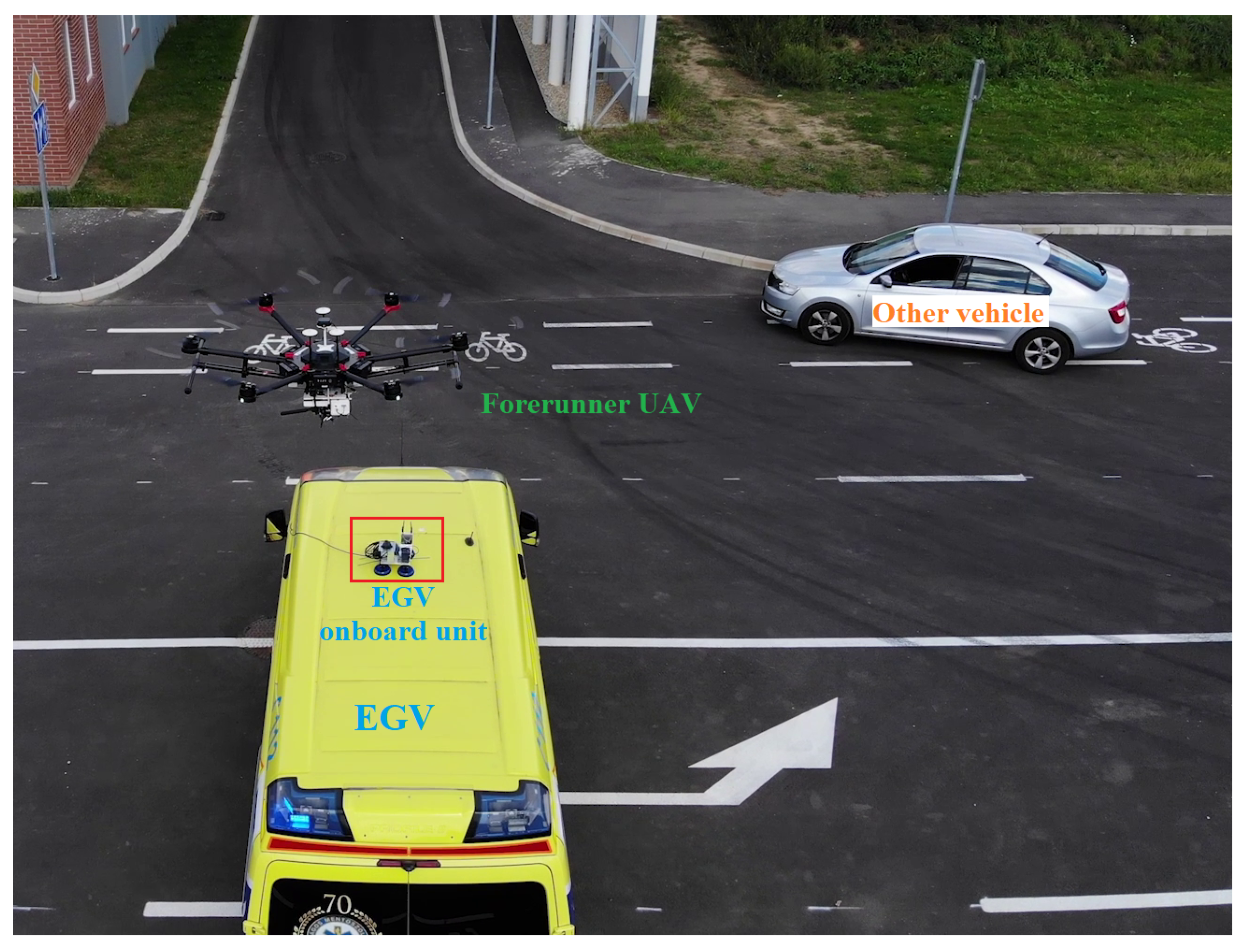
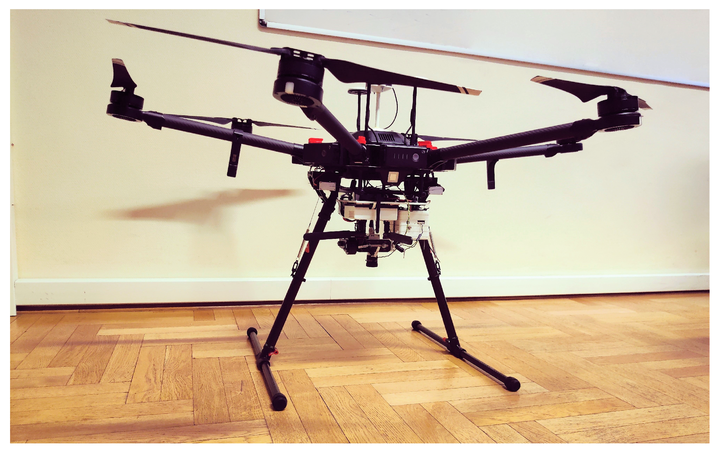
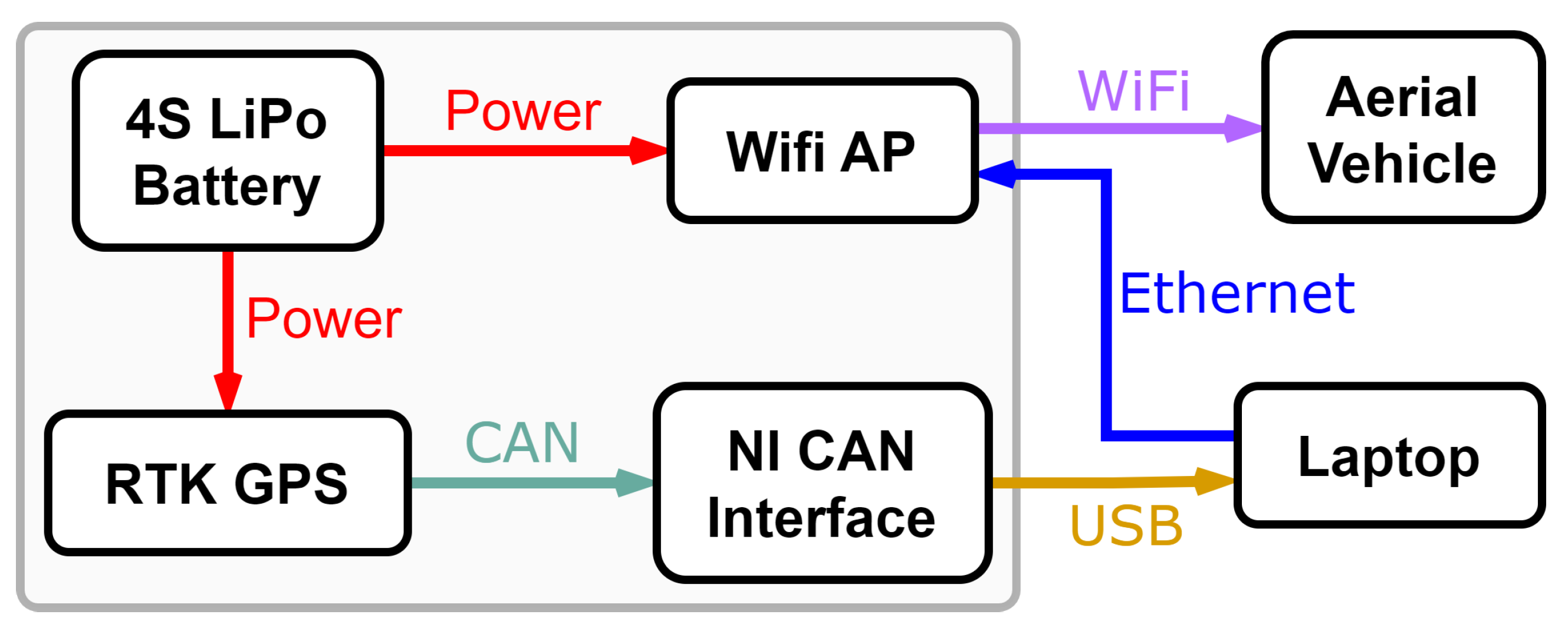
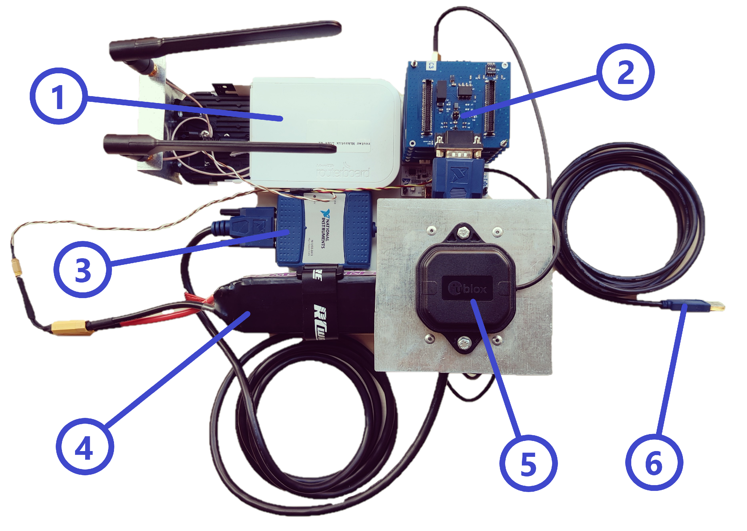
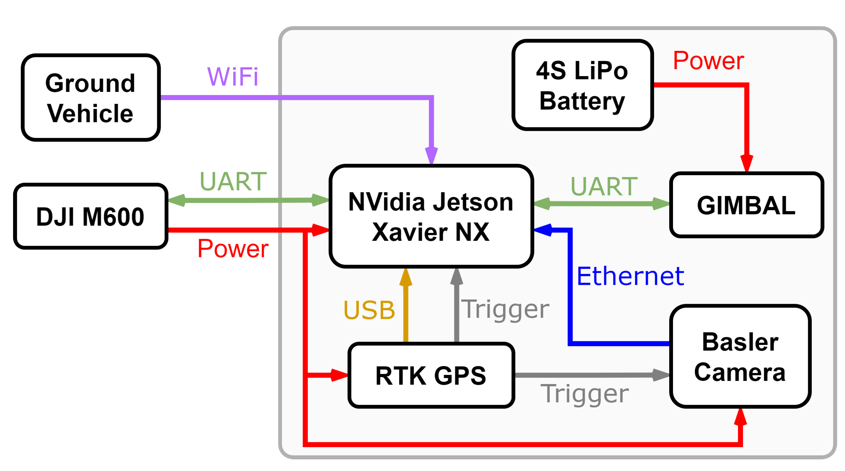
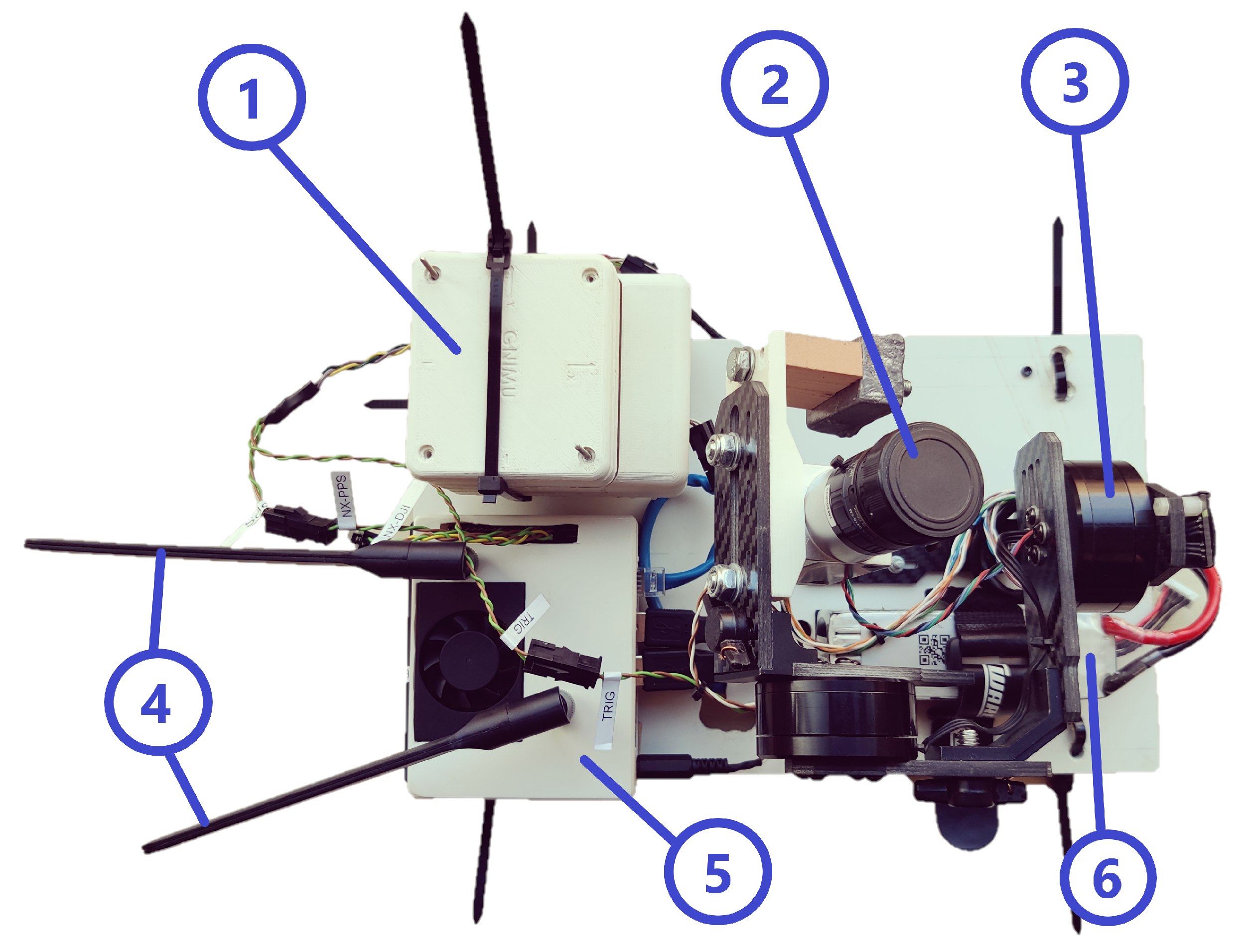
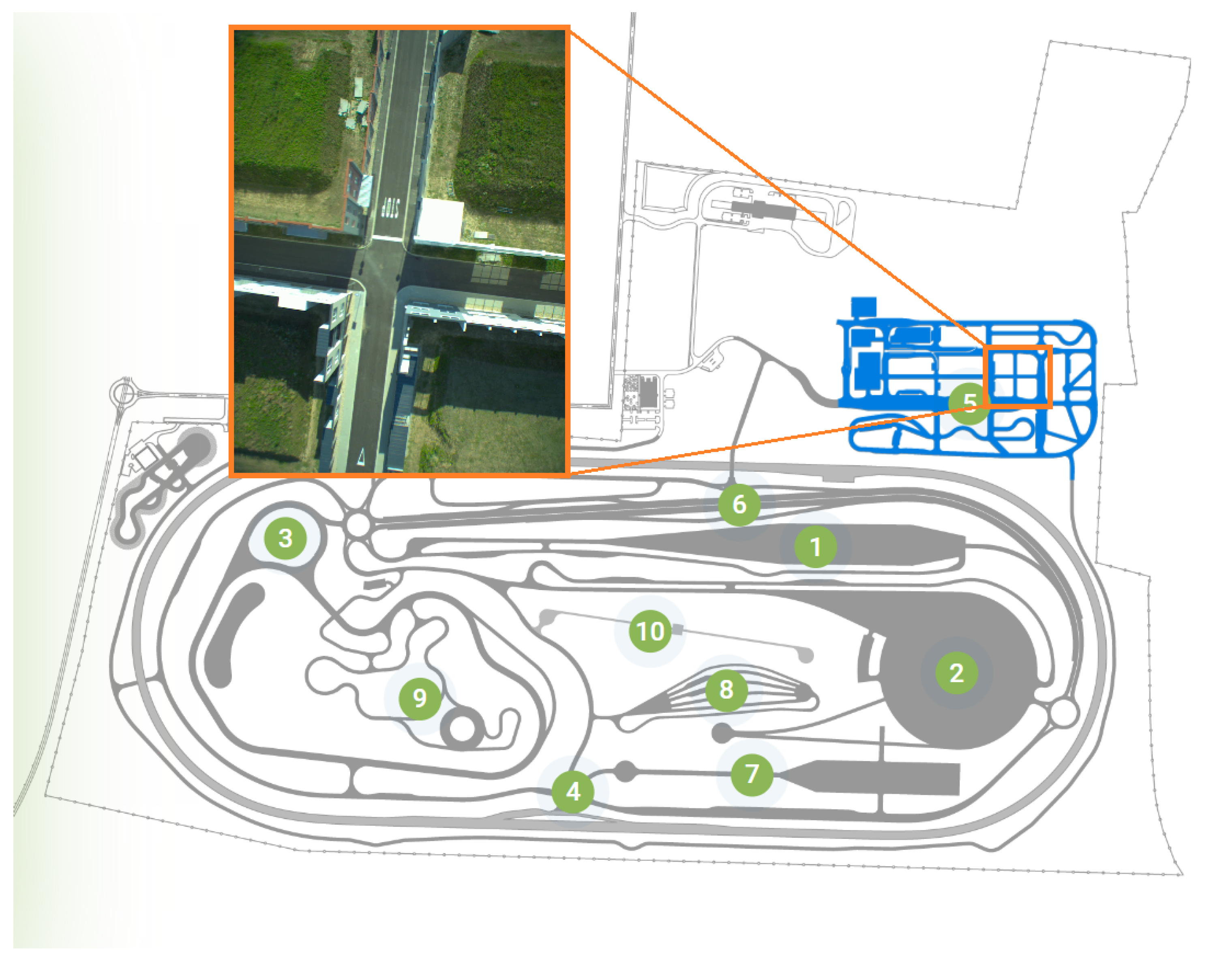
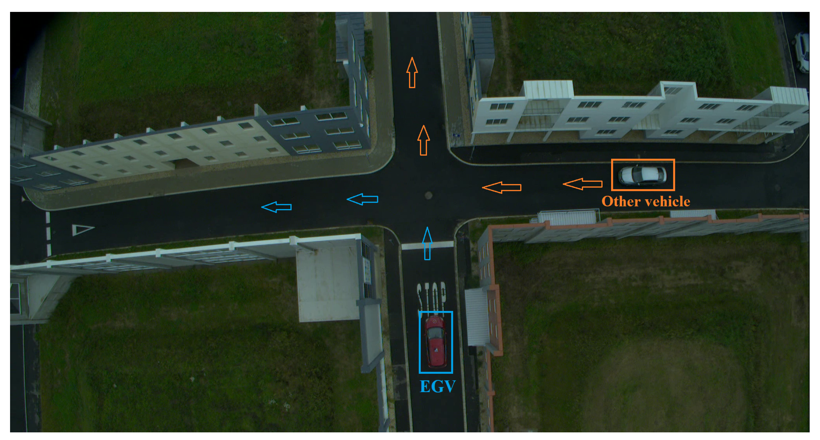
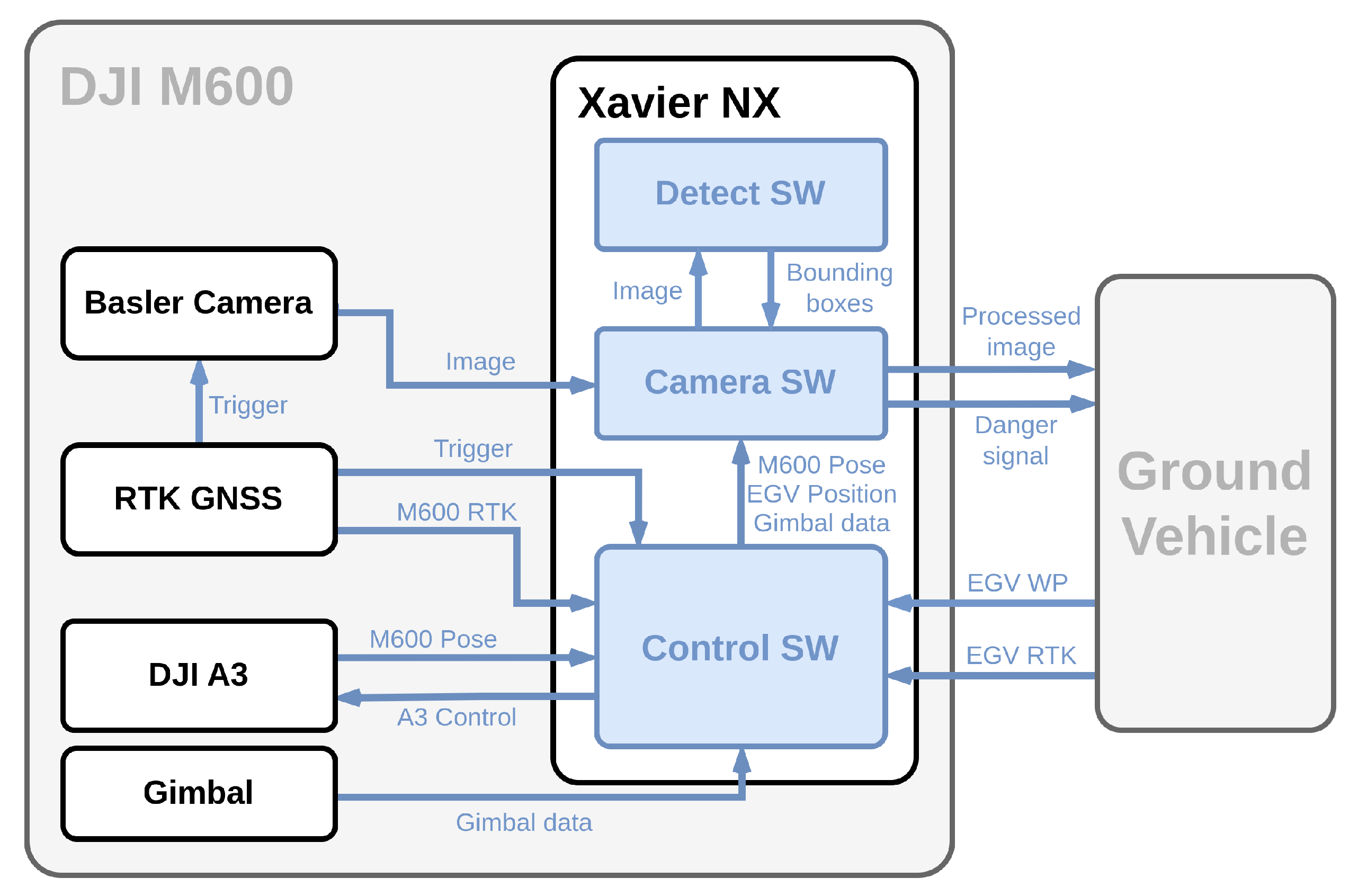
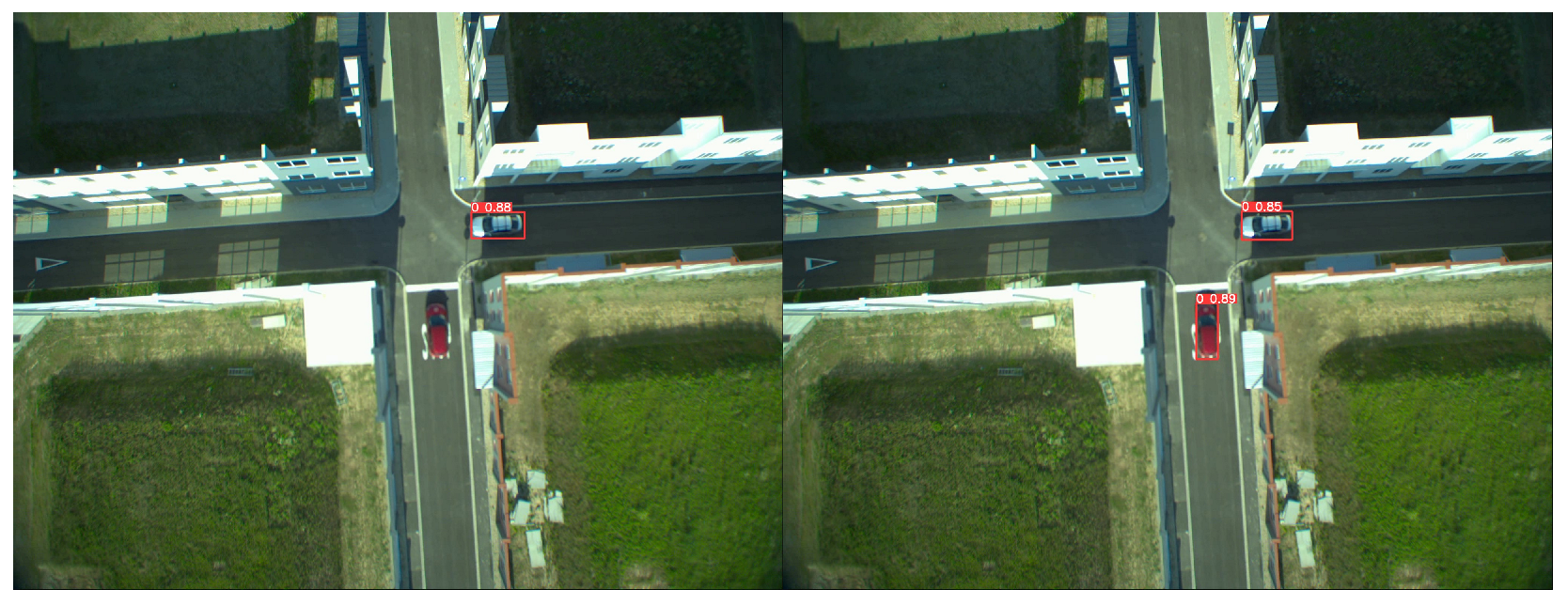
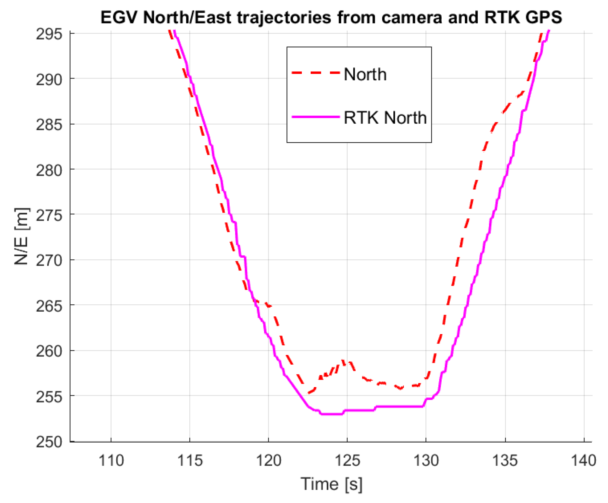
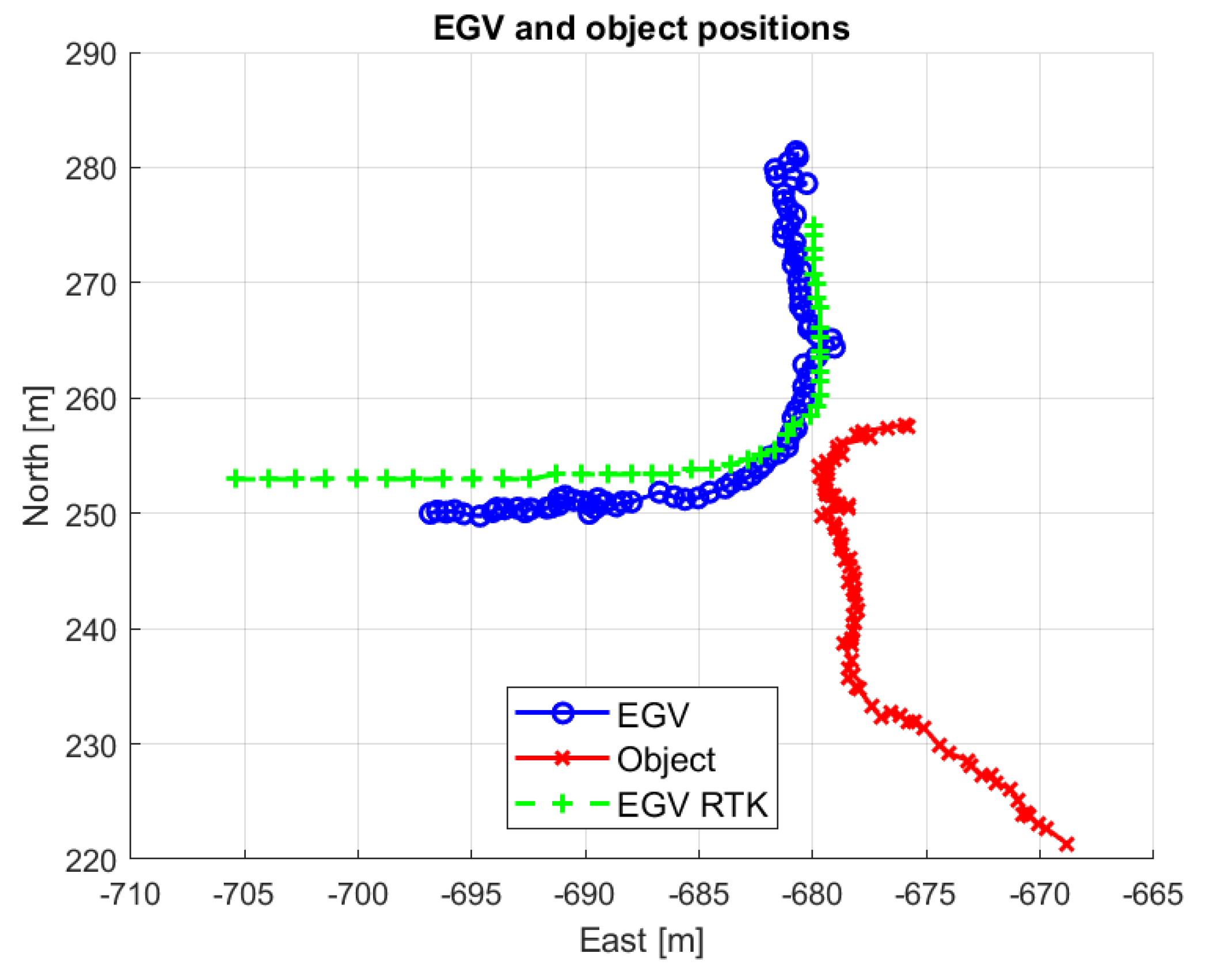
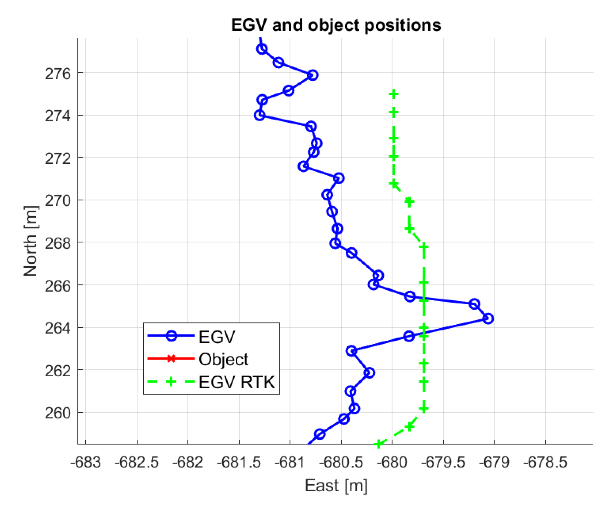
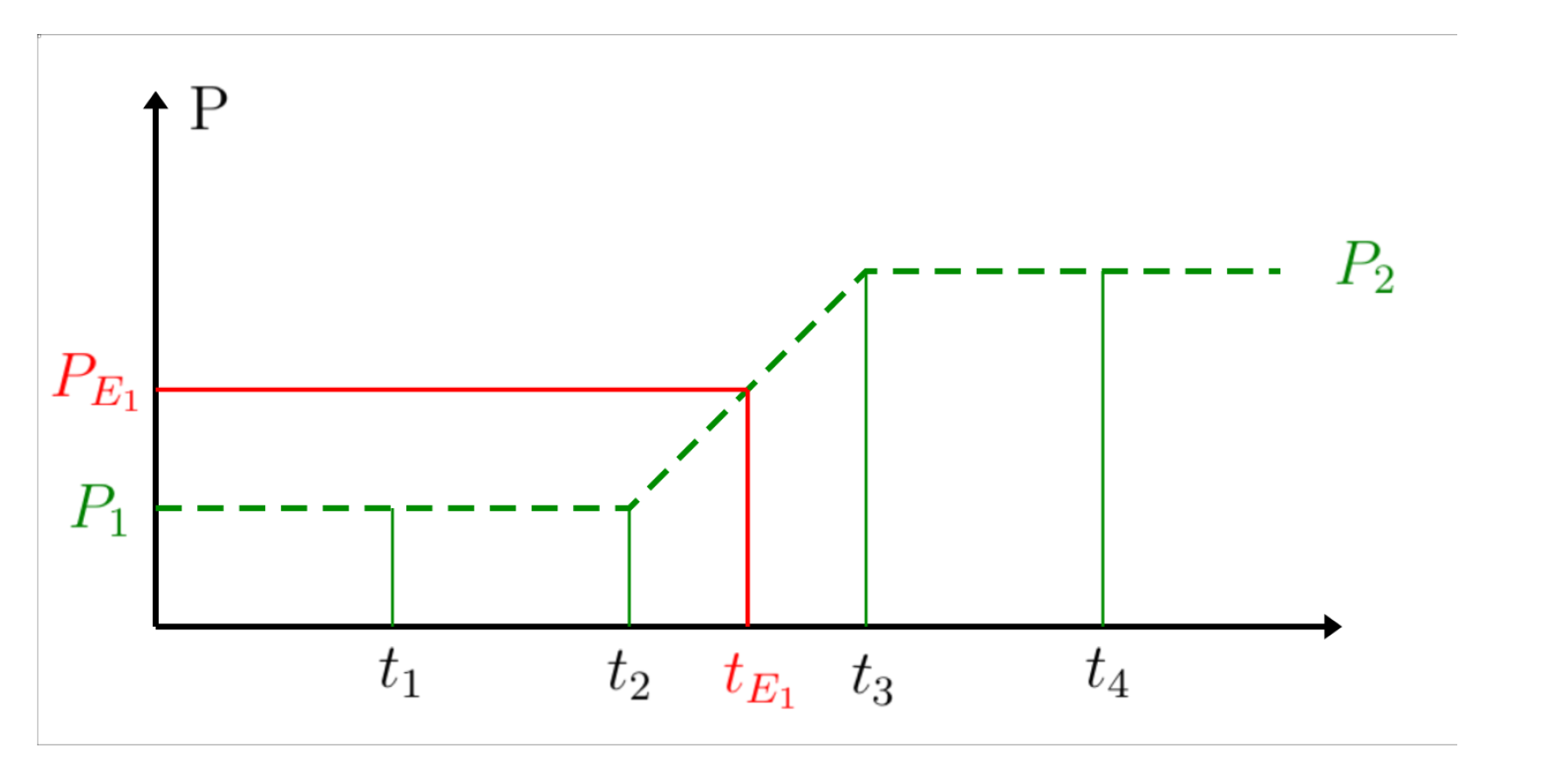
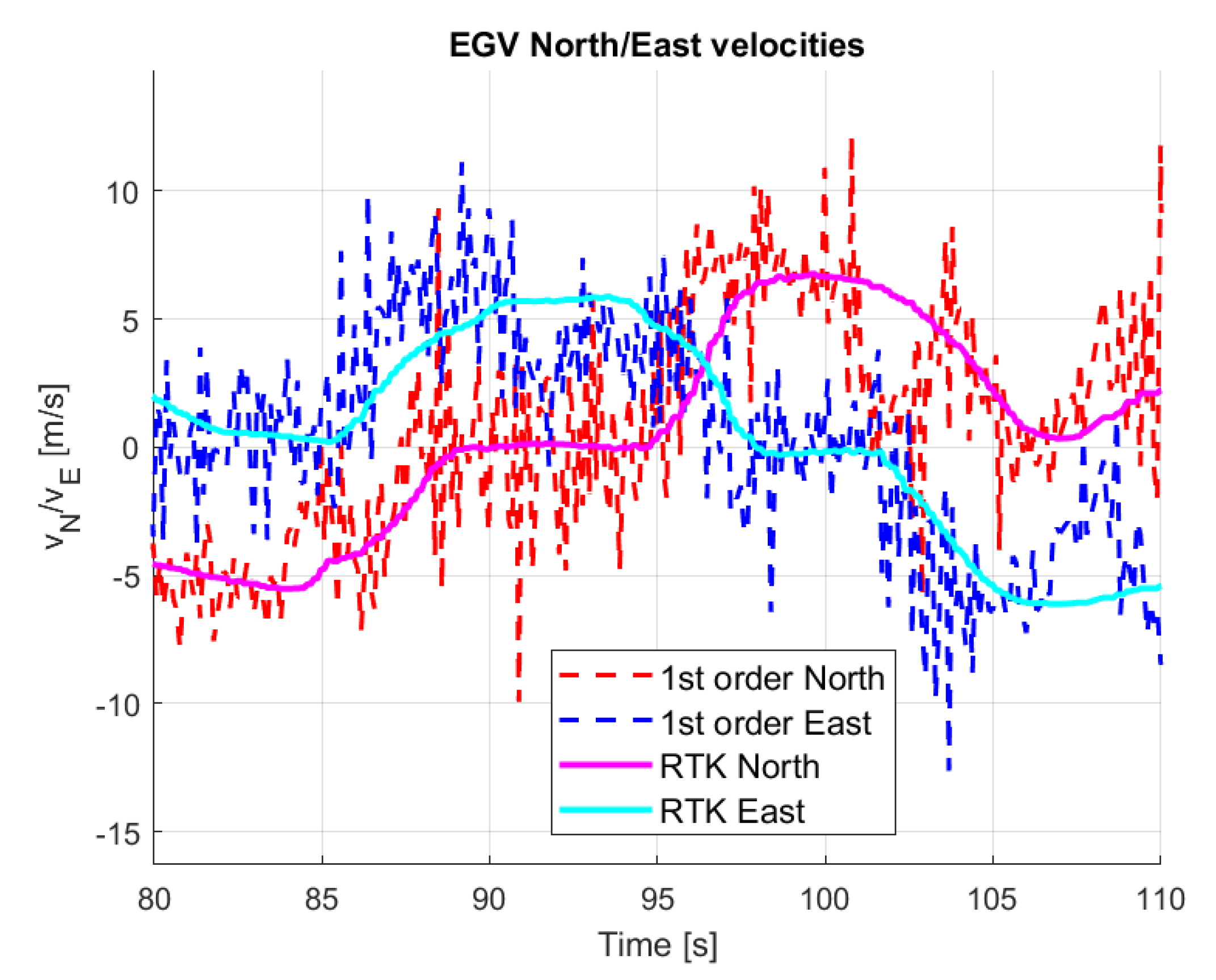
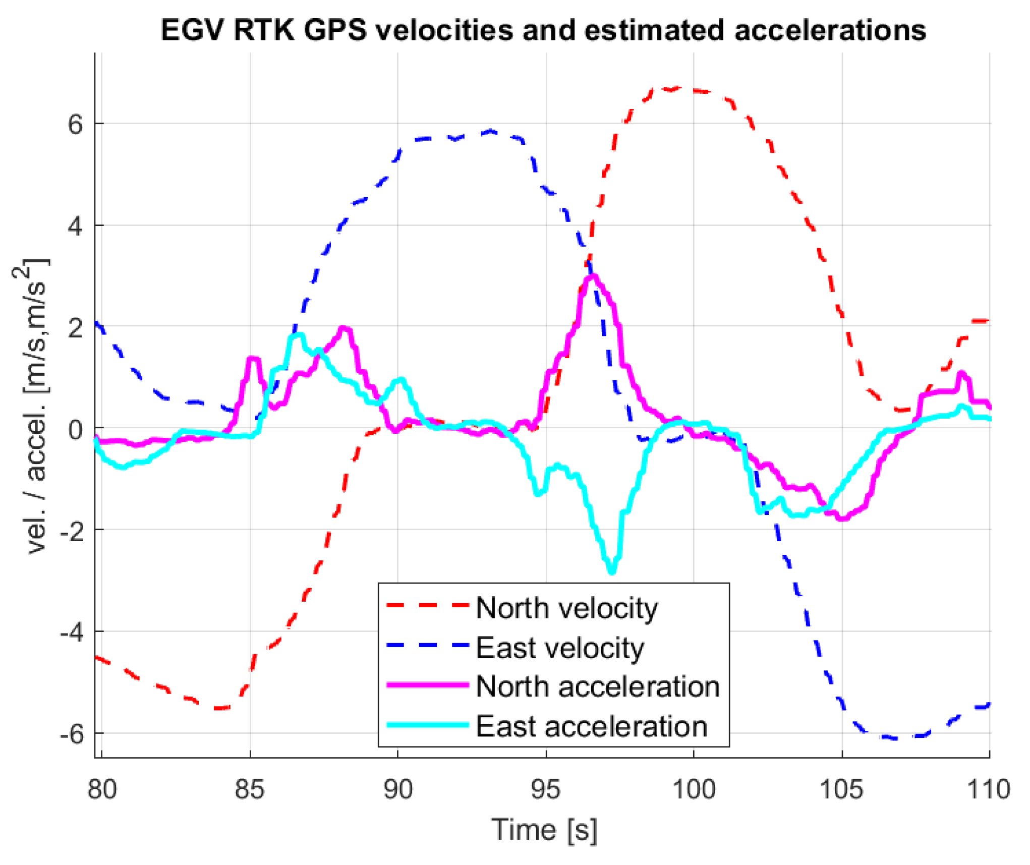
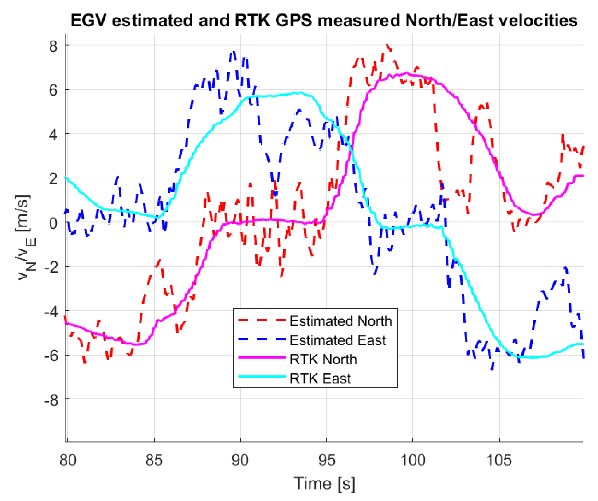
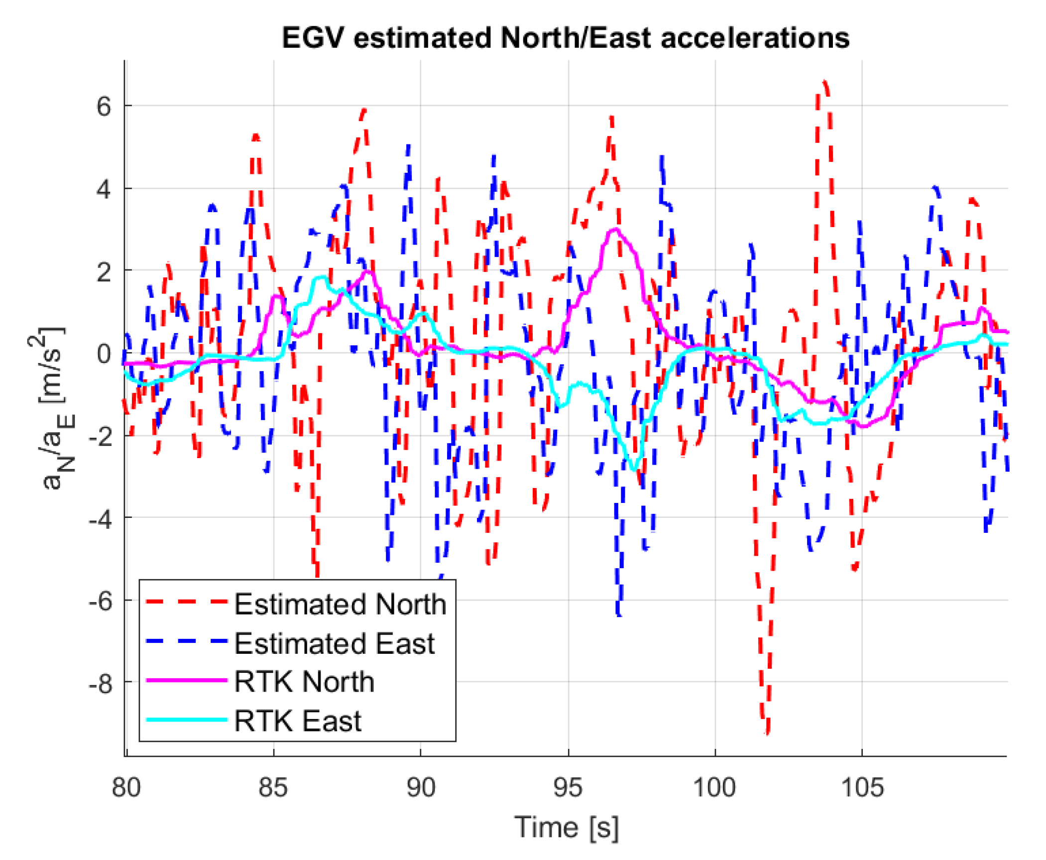
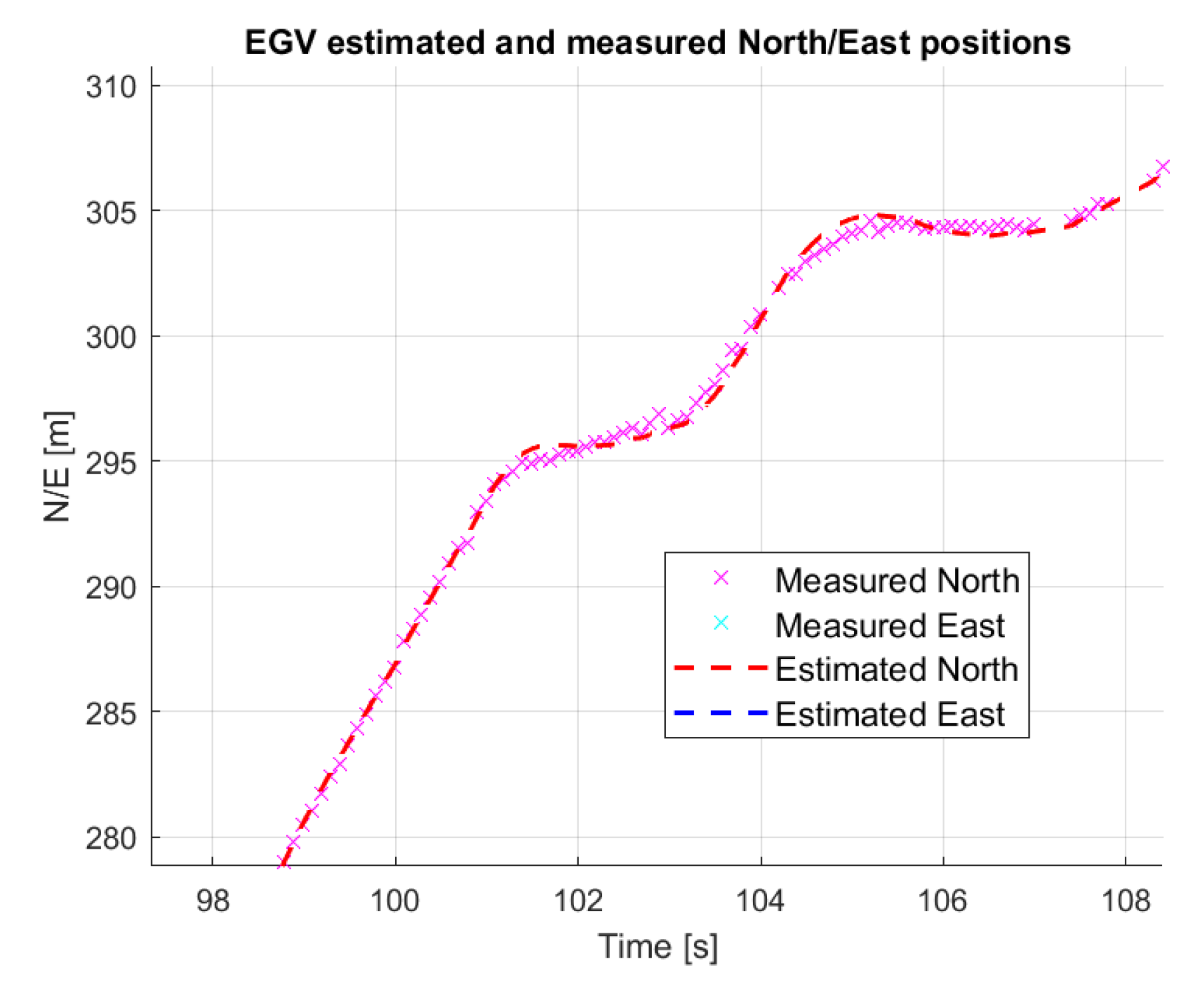
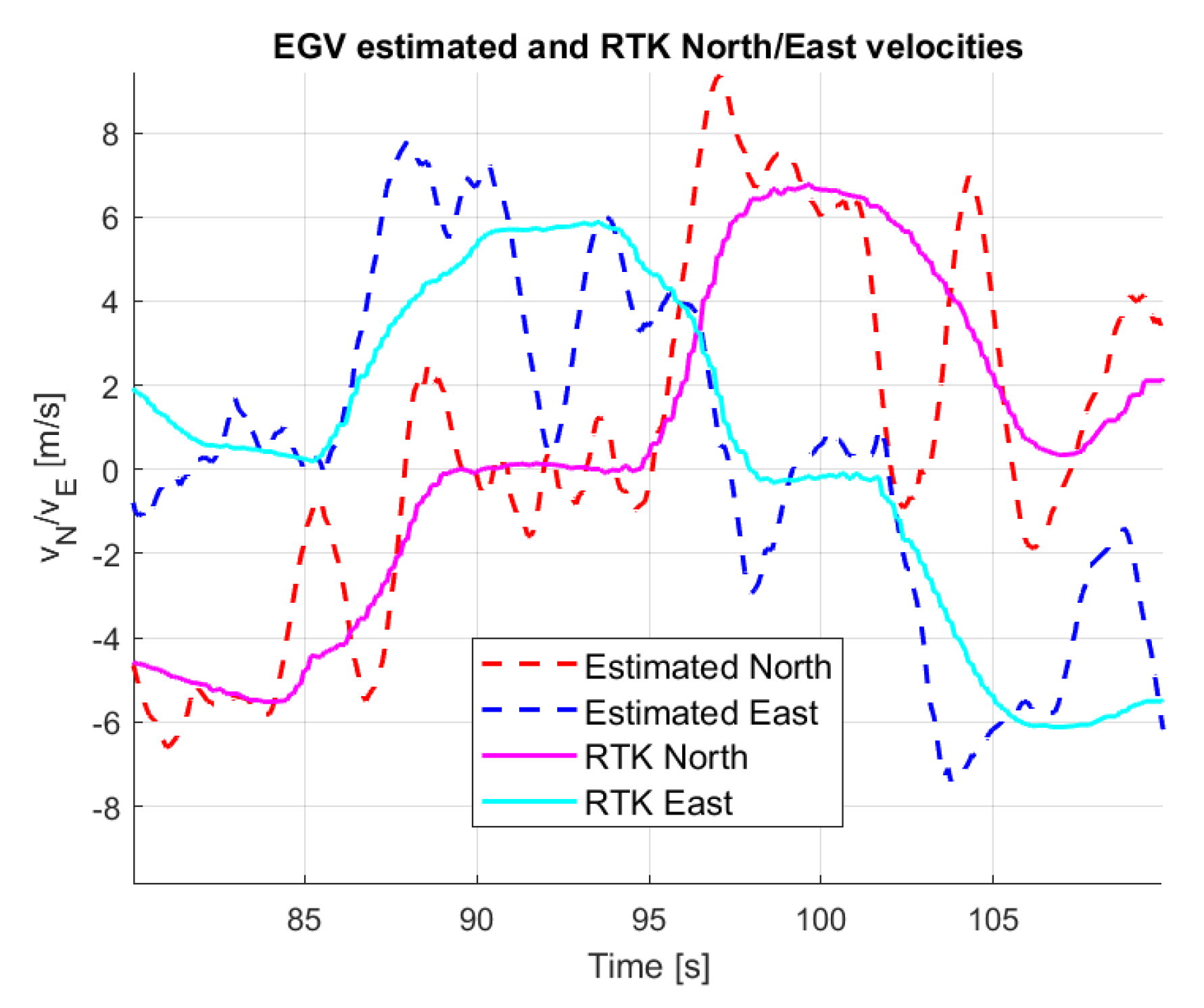
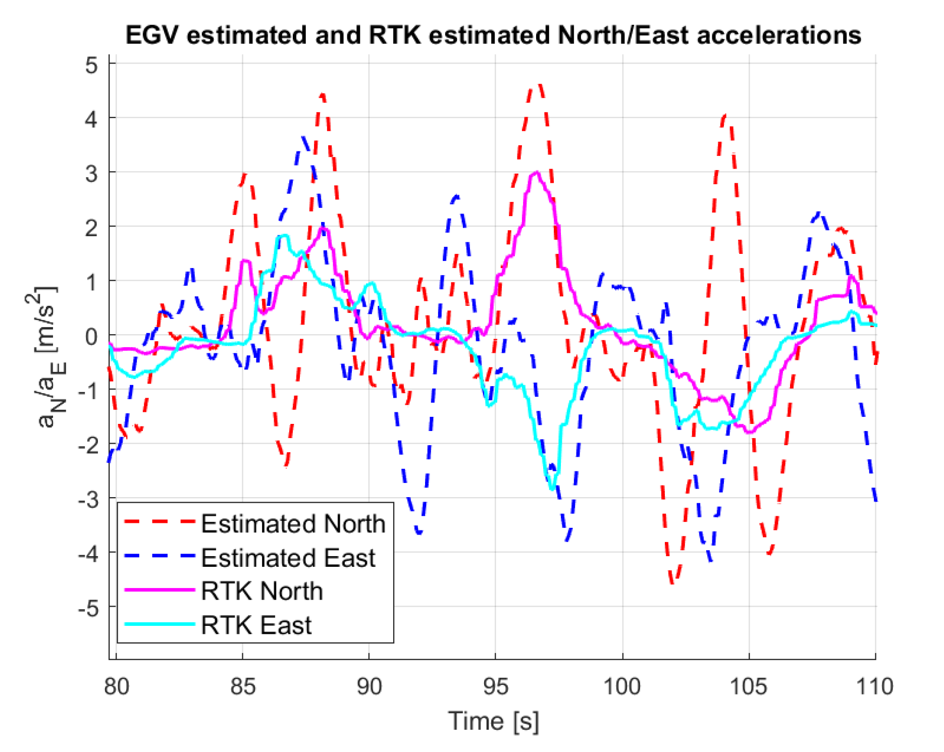
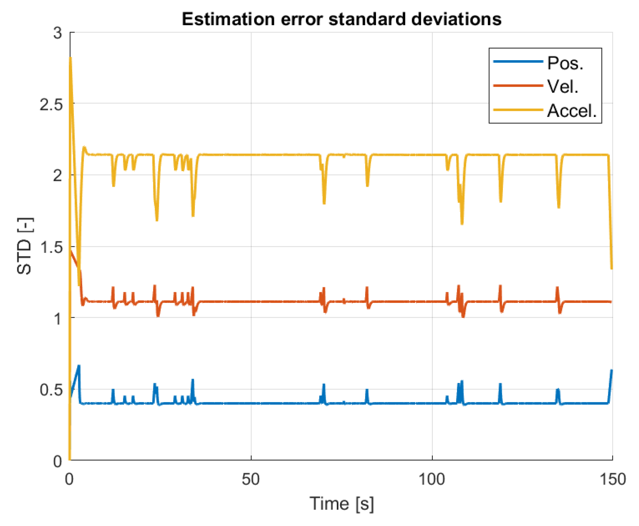
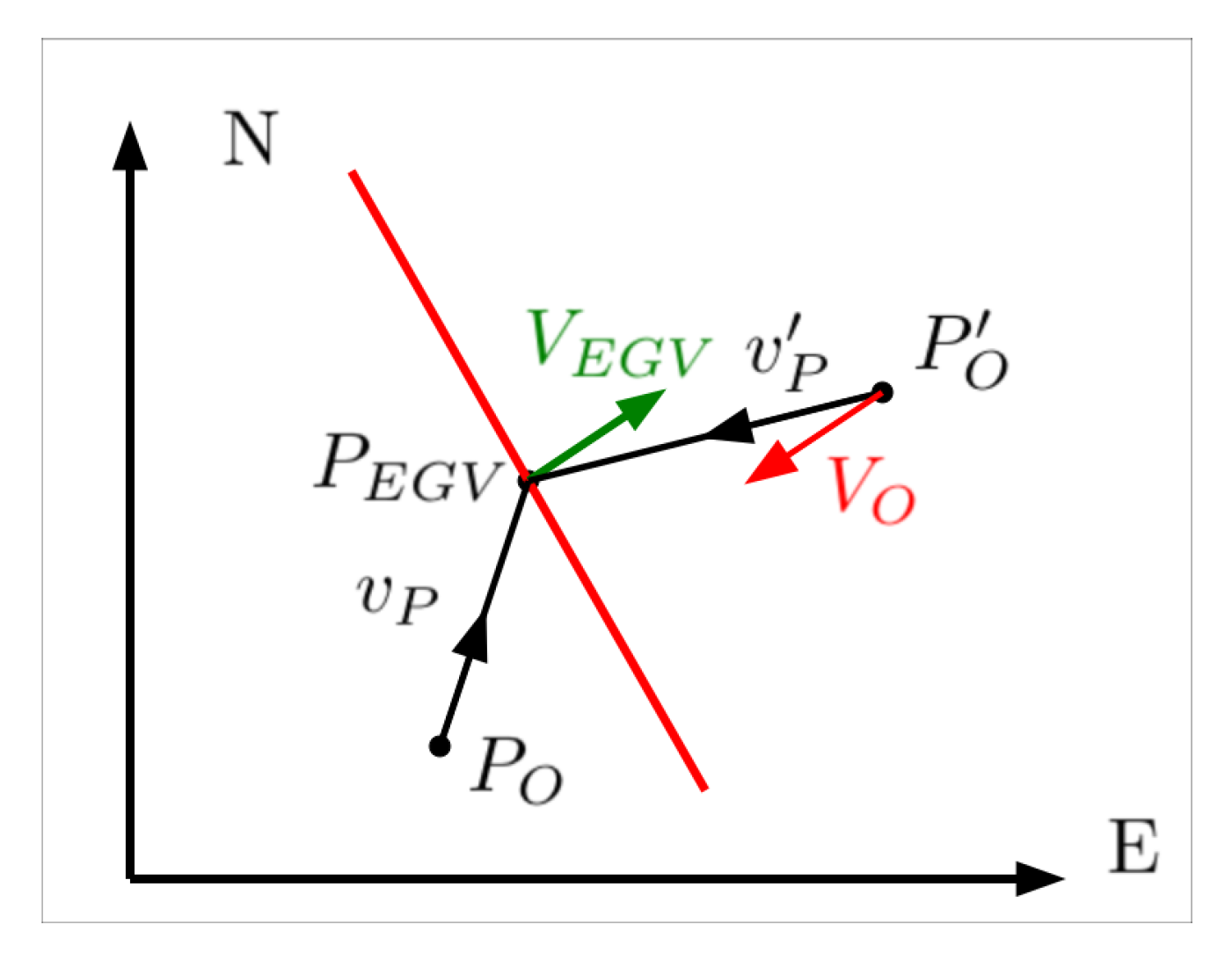
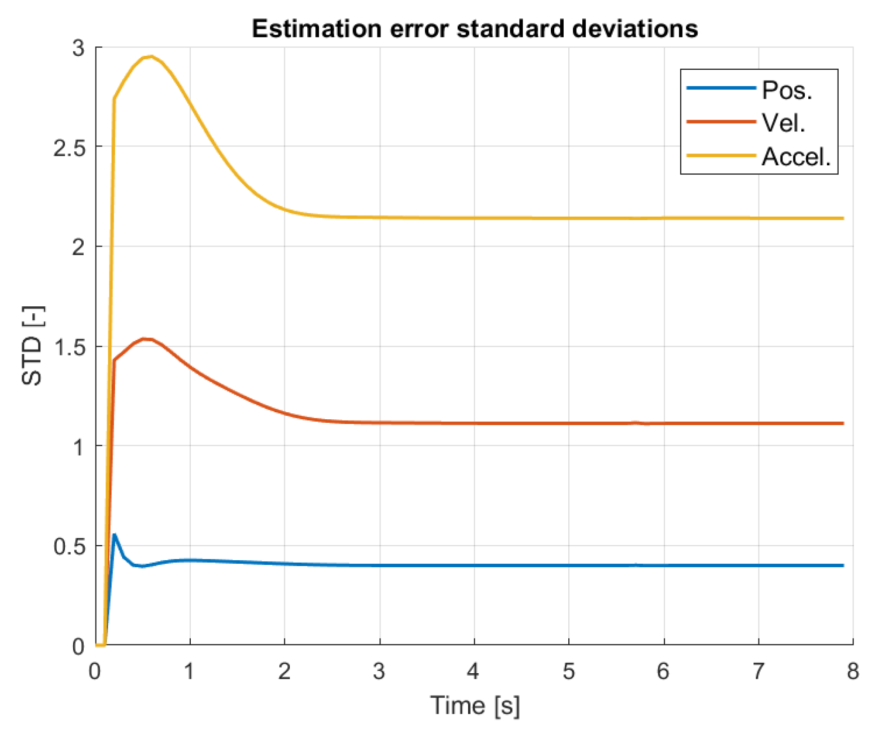
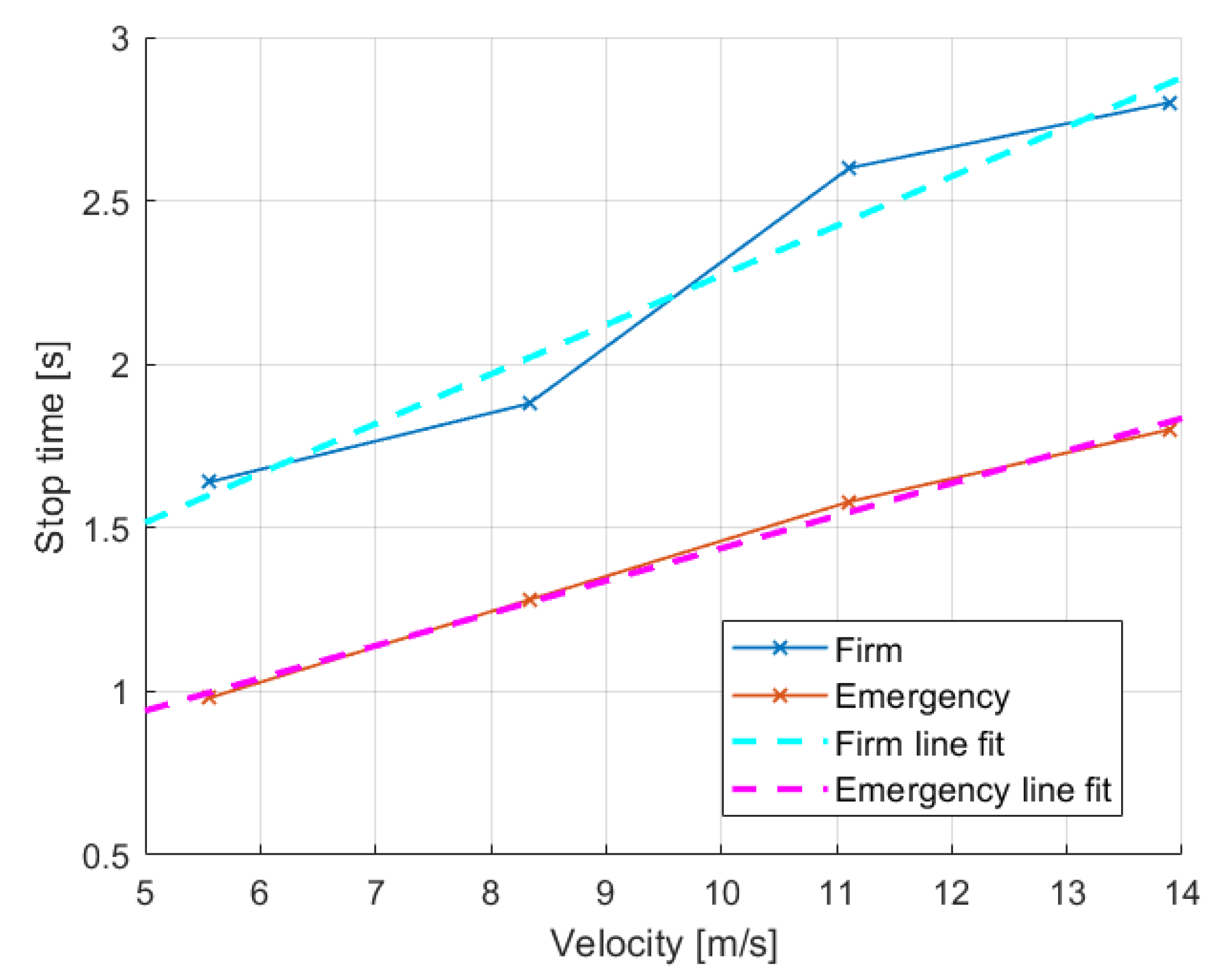
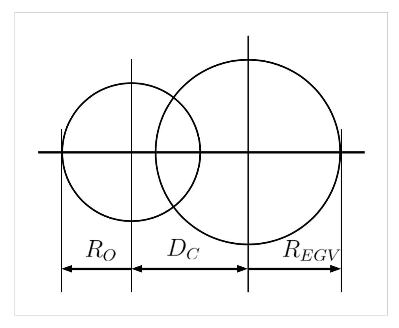
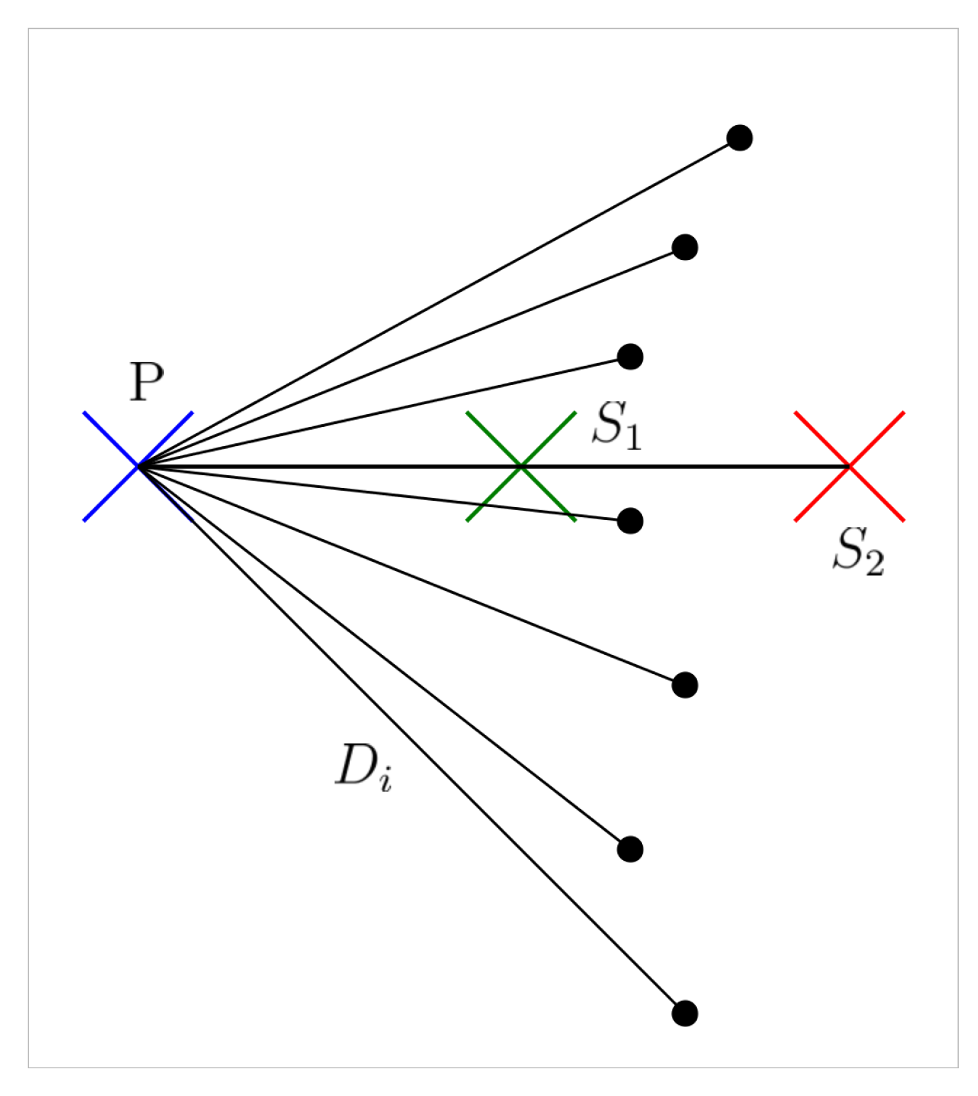
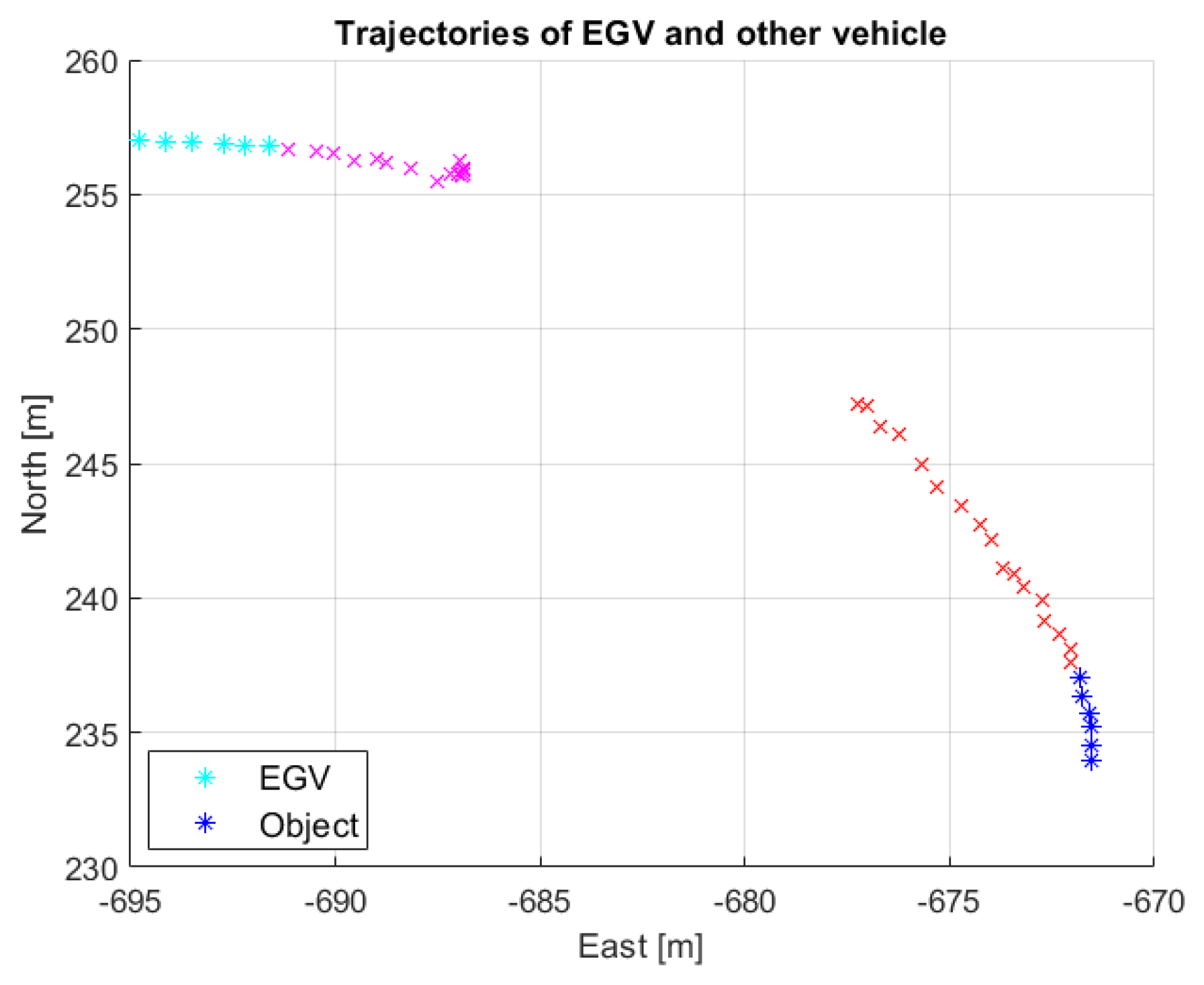
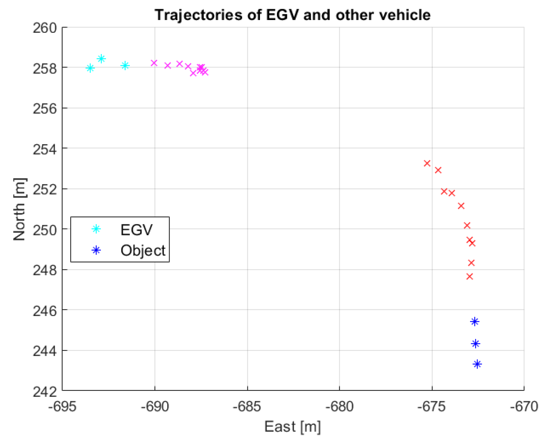
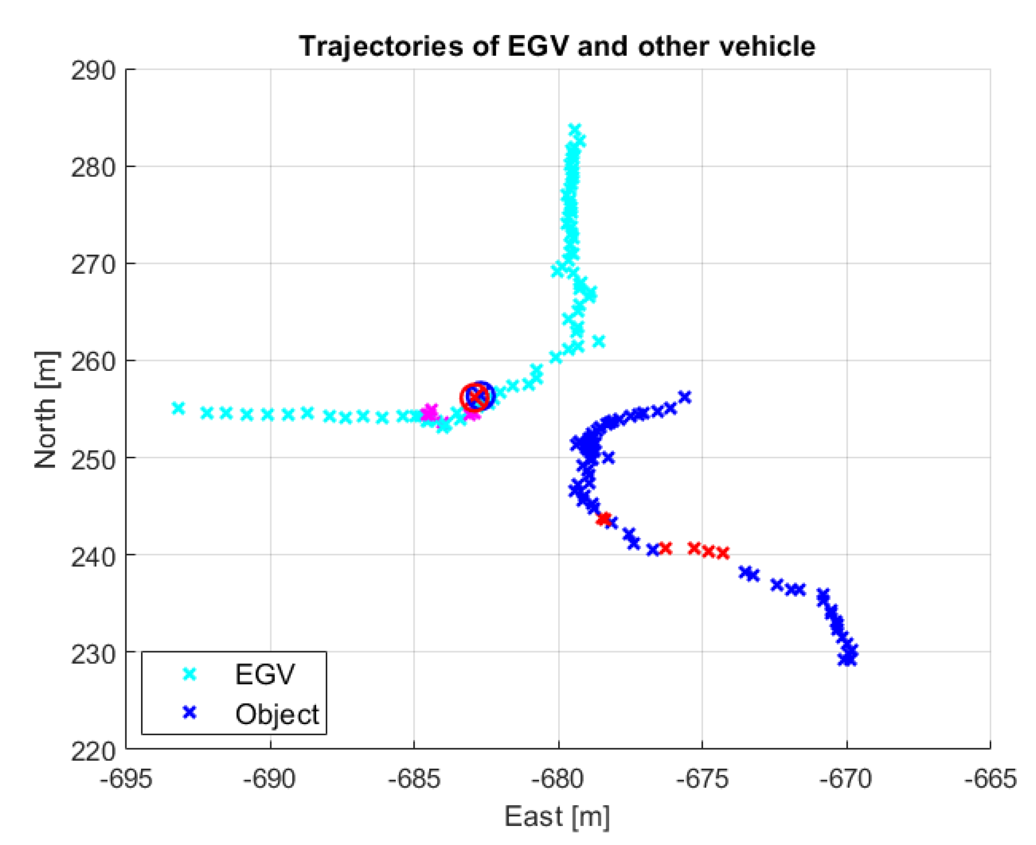
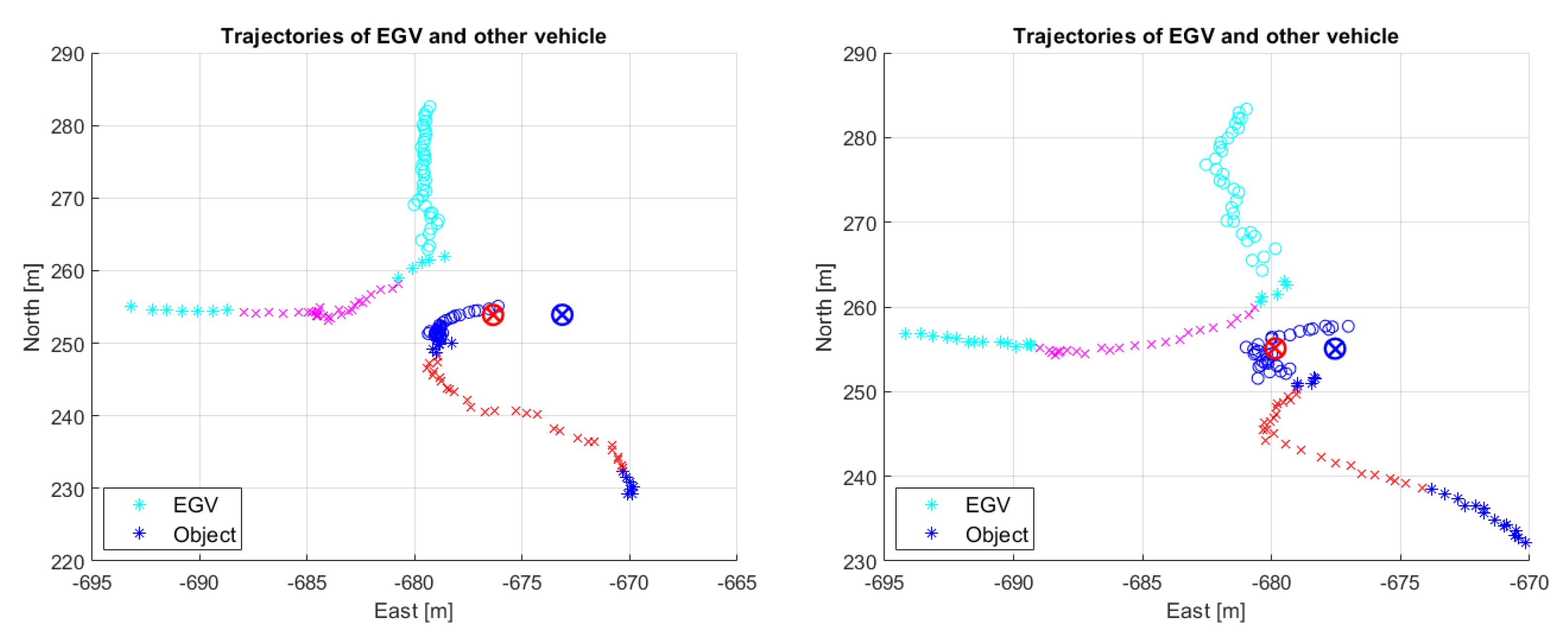
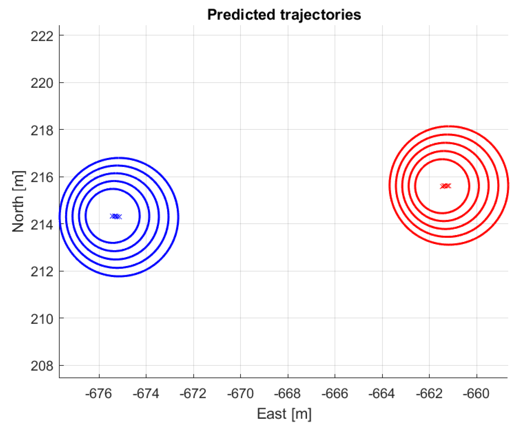
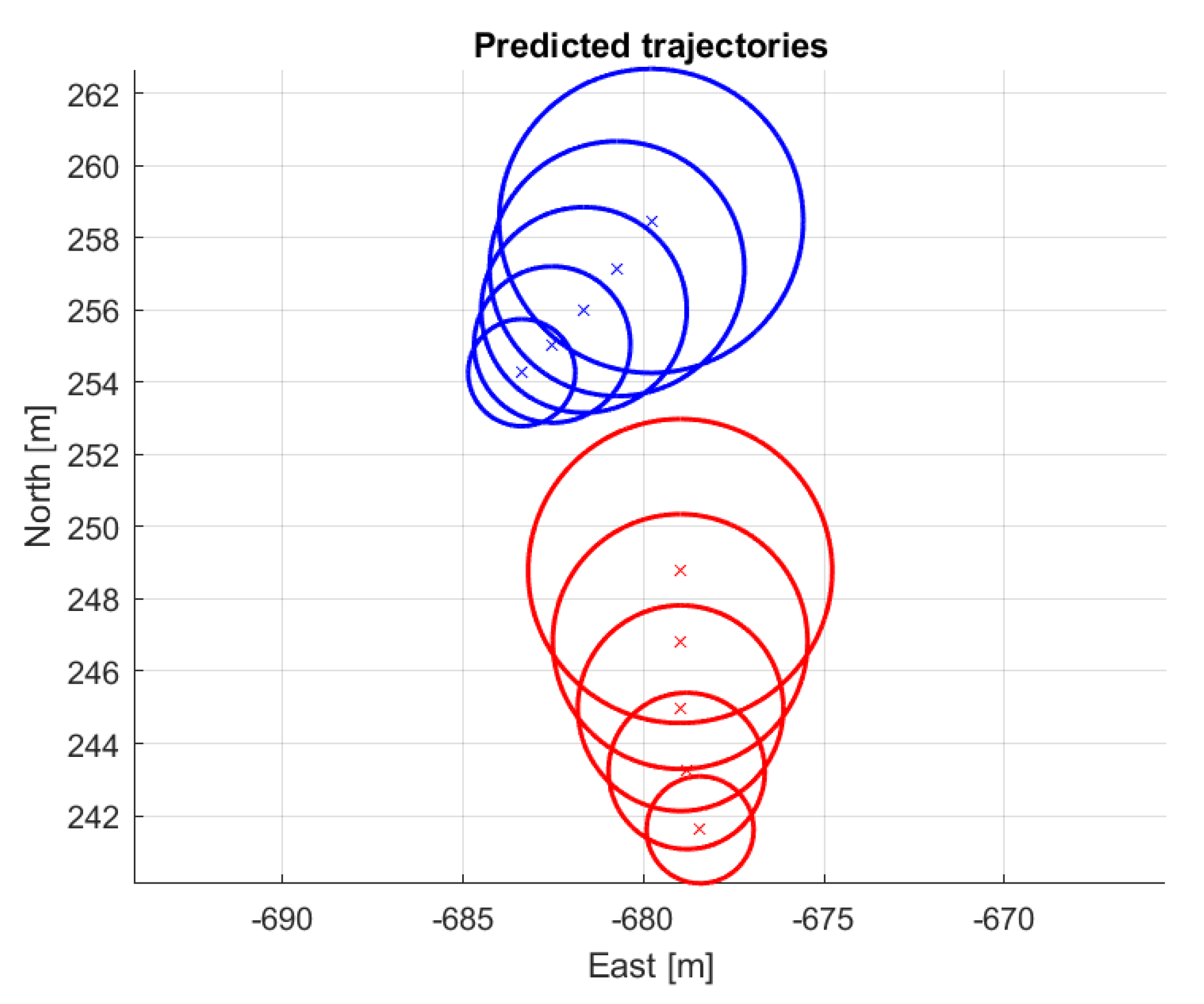
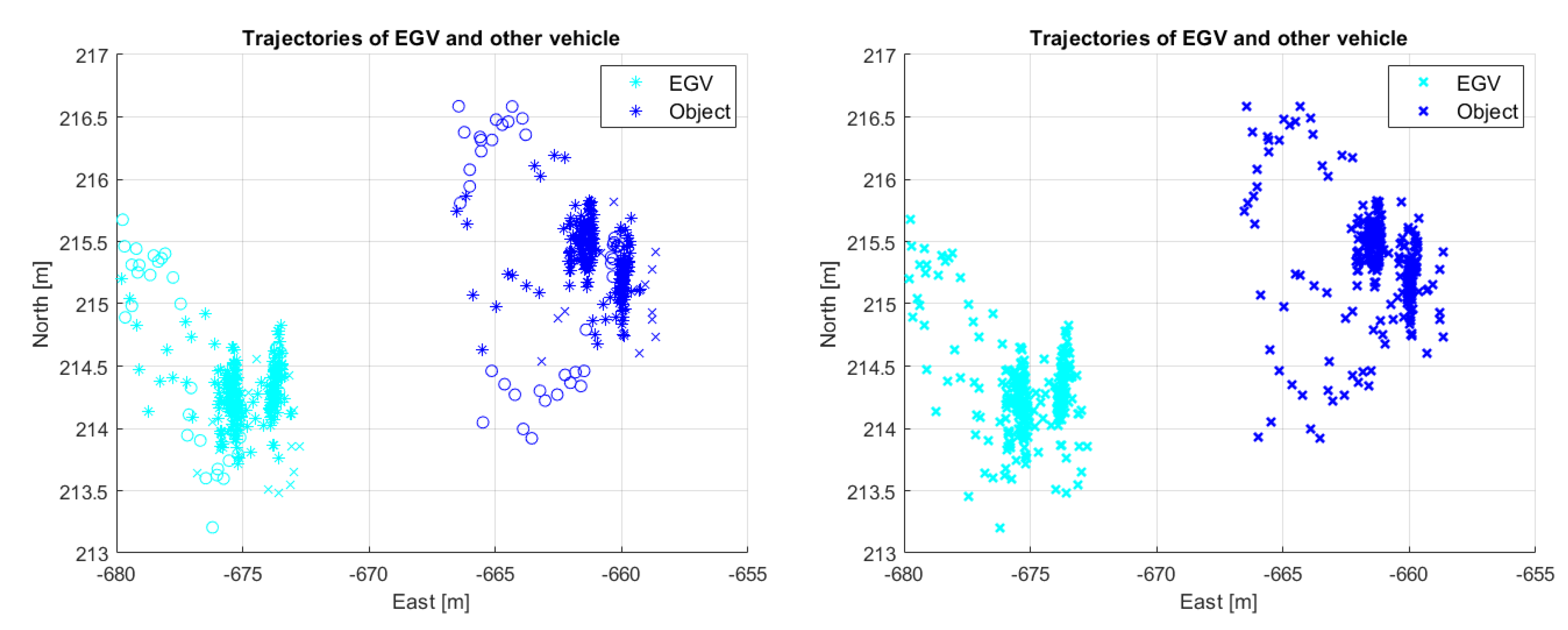
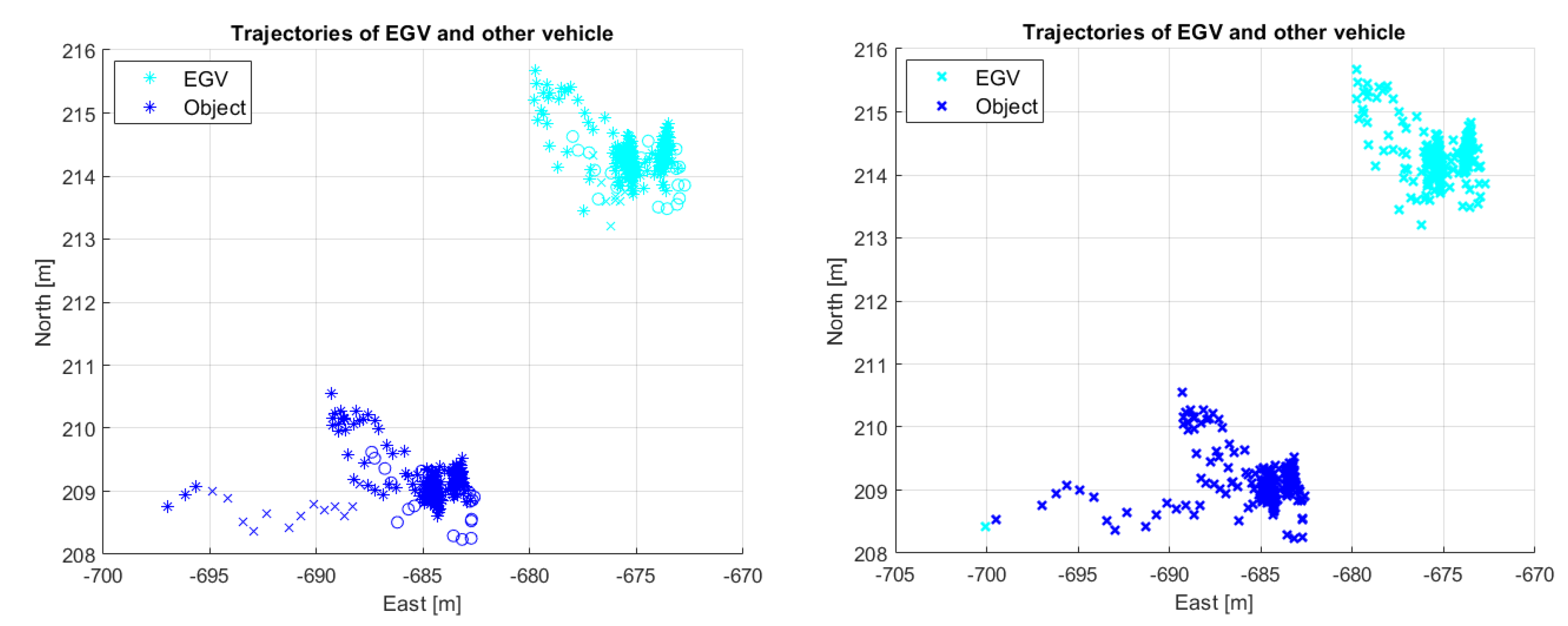
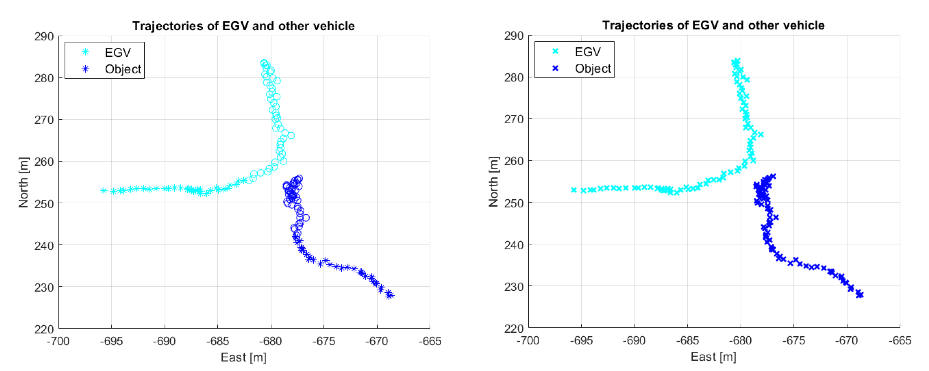
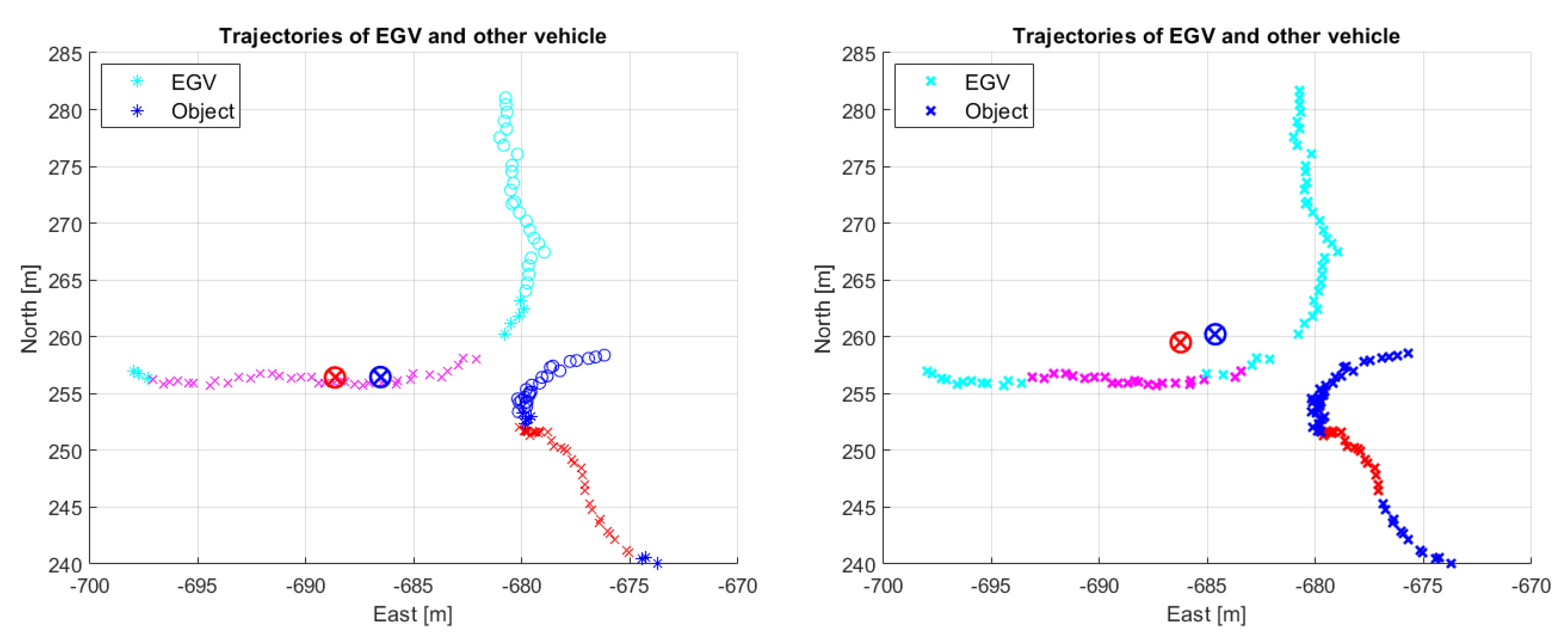
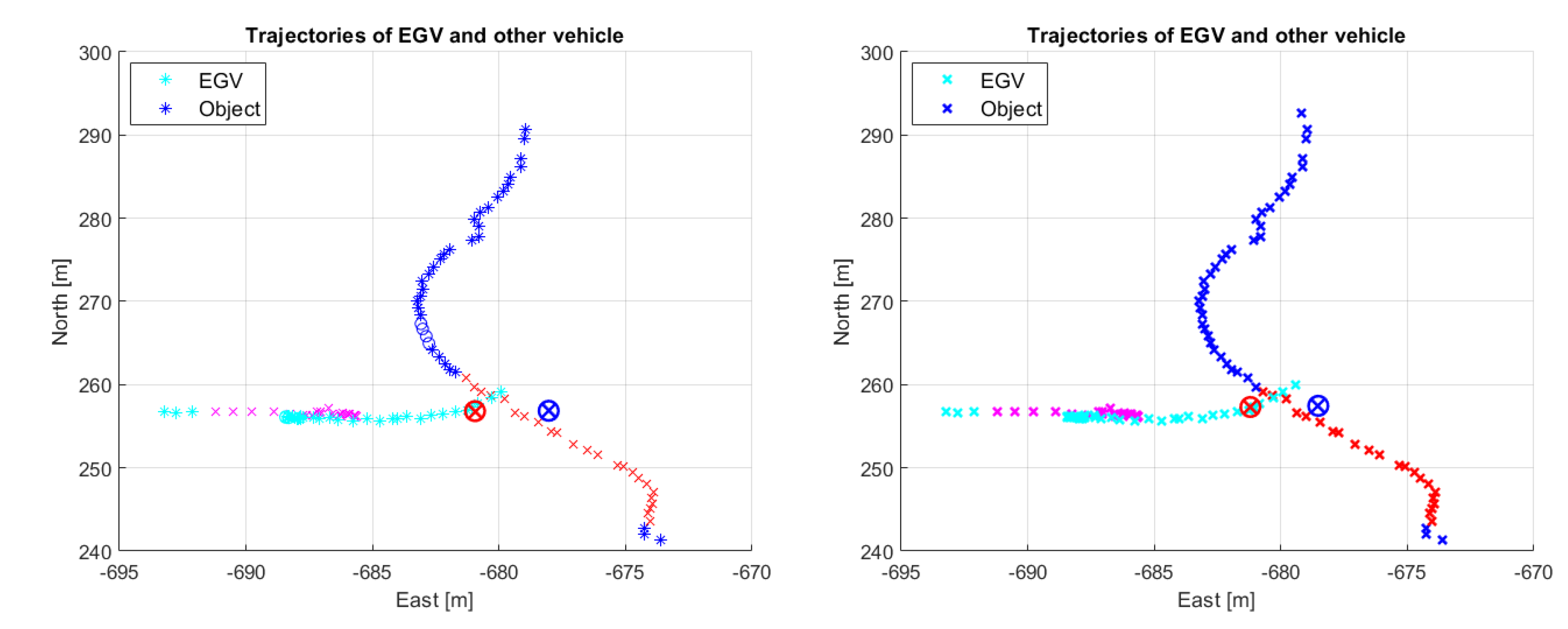
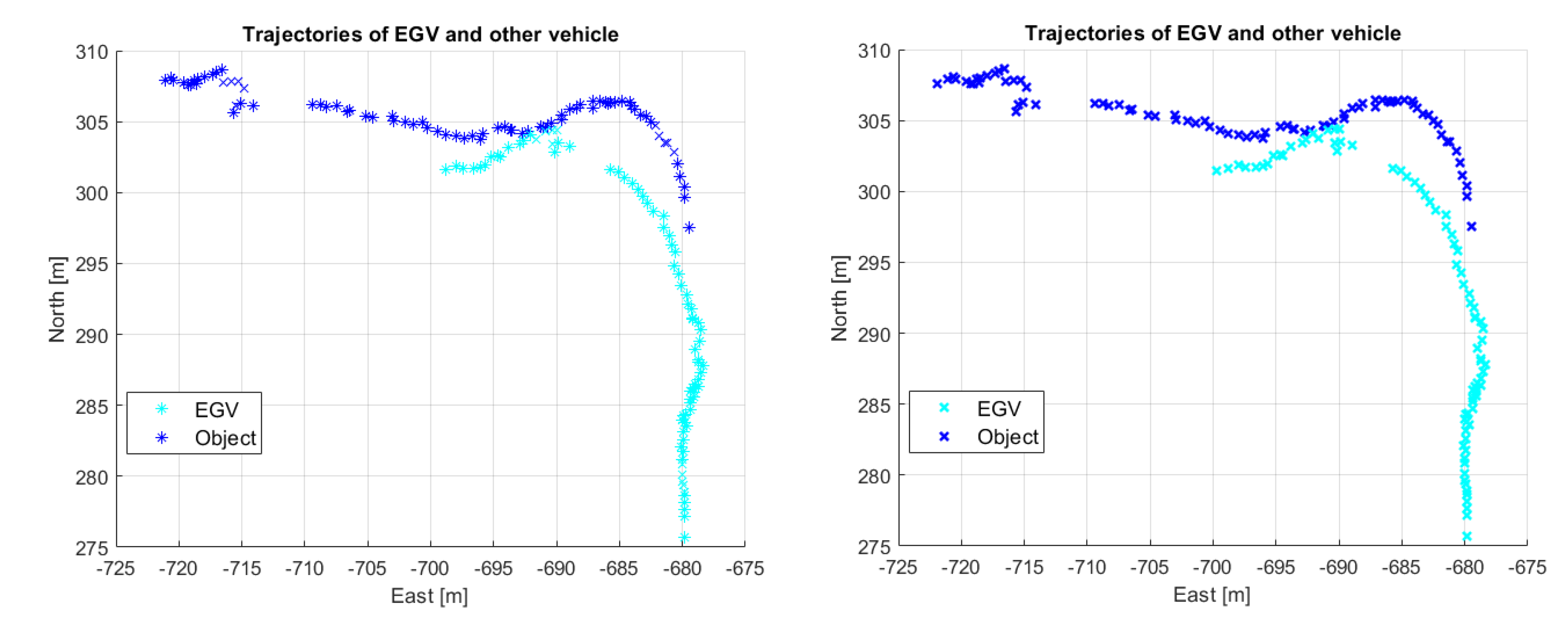
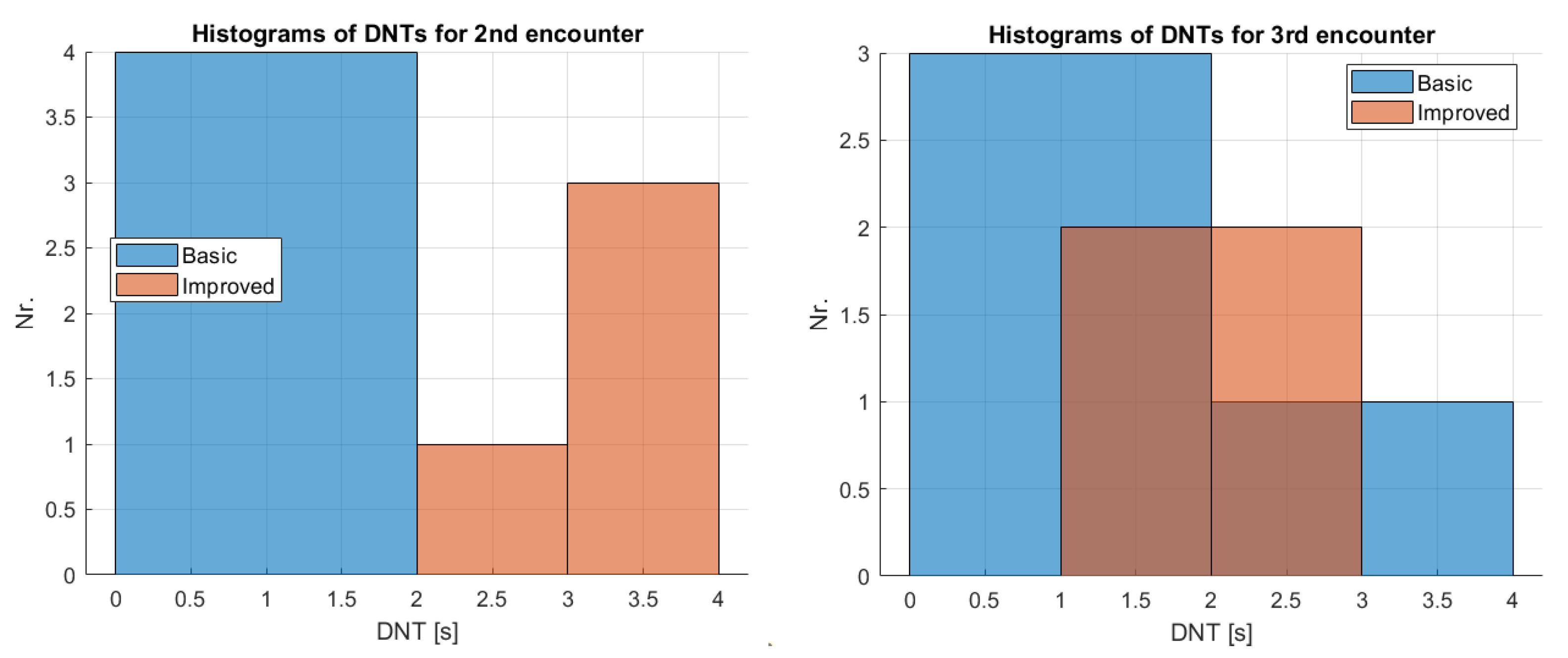
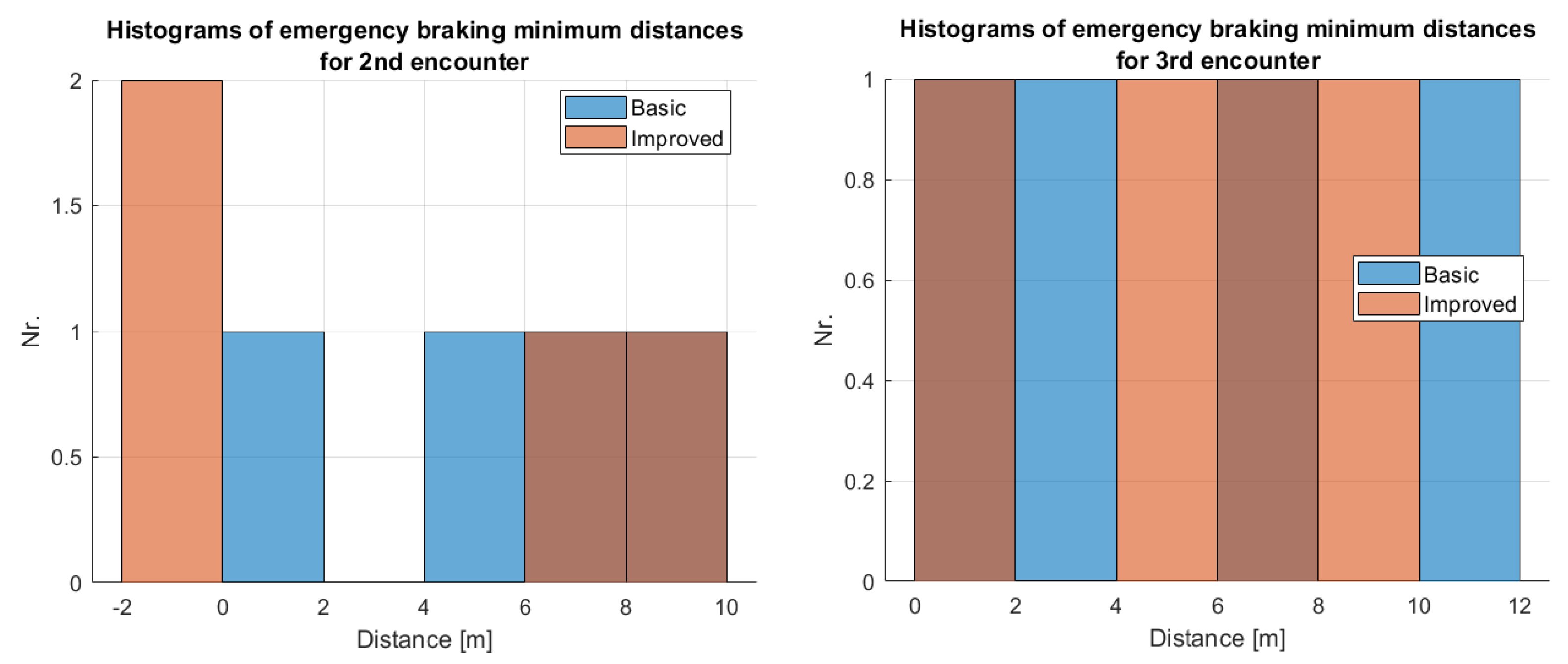
Table 1.
Training results for Yolov5s neural network trained on the CARLA dataset.
| Classes | Precision | Recall | F1 | [email protected] | mAP.5:0.95 |
|---|---|---|---|---|---|
| All | 0.938 | 0.826 | 0.878 | 0.878 | 0.581 |
| Cars | 0.941 | 0.979 | 0.959 | 0.977 | 0.827 |
| Bicycles | 0.938 | 0.861 | 0.897 | 0.918 | 0.54 |
| Pedestrians | 0.934 | 0.637 | 0.757 | 0.739 | 0.377 |
Table 2.
Training results for the Yolo_RL network.
| Classes | Precision | Recall | F1 | [email protected] | mAP.5:0.95 |
|---|---|---|---|---|---|
| Cars | 0.941 | 0.94 | 0.94 | 0.95 | 0.775 |
Table 3.
Position measurement error variances.
| Direction | Flight 1 | Flight 2 | Flight 3 | Flight 4 | Average |
|---|---|---|---|---|---|
| North | 0.058 | 0.26 | 0.315 | 0.0662 | 0.1748 |
| East | 1.43 | 0.93 | 0.333 | 0.2 | 0.7233 |
Table 4.
Maximum braking times of a car [s].
| Braking Type | 20 km/h | 30 km/h | 40 km/h | 50 km/h |
|---|---|---|---|---|
| Firm | 1.64 | 1.88 | 2.6 | 2.8 |
| Emergency | 0.98 | 1.28 | 1.58 | 1.8 |
Table 5.
Tuning parameters for basic decision method.
| Parameter | MIN | Step | MAX |
|---|---|---|---|
| W [-] | 3 | 1 | 9 |
| [s] | 1 | 0.5 | 2.5 |
| [m] | 2 | 2 | 6 |
| [-] | 2 | 2 | 8 |
Table 6.
Combination of braking styles in decision and evaluation.
| Notation | Decision Braking Style | Evaluation Braking Style |
|---|---|---|
| FF | Firm | Firm |
| EE | Emergency | Emergency |
| FE | Firm | Emergency |
Table 7.
Tuning parameters for improved decision method.
| Parameter | MIN | Step | MAX |
|---|---|---|---|
| [-] | 1 | 1 | 3 |
| [-] | 1 | 1 | 3 |
| [s] | −0.2 | 0.1 | 0.2 |
| [-] | 0 | 0.1 | 0.5 |
| FF | - | - | - |
| EE | - | - | - |
| FE | - | - | - |
Table 8.
Resulting valid basic method parameters from flight 1.
| W [-] | [s] | [m] | [-] |
|---|---|---|---|
| 4 | 1.5 | 6 | 8 |
| 4 | 2 | 2 | 6 |
| 4 | 2 | 2 | 8 |
Table 9.
Resulting valid improved method parameters from flights 1 and 2 with firm decision and emergency evaluation.
Table 9.
Resulting valid improved method parameters from flights 1 and 2 with firm decision and emergency evaluation.
| Valid Combination | S1 | S2 | S3 | S4 | S5 | S6 |
|---|---|---|---|---|---|---|
| Flight 2/3rd Enc. | ||||||
| 1 | 1 | 2 | 2 | 3 | 3 | |
| 2 | 3 | 2 | 3 | 2 | 3 | |
| [m] | 4.83 | 5.45 | 4.83 | 5.68 | 5.28 | 5.92 |
| DNT () [s] | 2.3 | 3.5 | 2.3 | 3.7 | 2.7 | 3.8 |
| Flight 1/3rd Enc. | ||||||
| Case | S1 | S2 | S3 | S4 | S5 | S6 |
| [m] | 1.46 | 1.46 | 1.46 | 1.46 | 1.46 | 1.46 |
| DNT () [s] | 2.2 | 2.6 | 2.4 | 2.6 | 2.4 | 2.7 |
| Flight 1/1st Enc. | ||||||
| Case | S1 | – | S3 | – | – | – |
| Flight 2/1st Enc. | ||||||
| Case | – | – | – | – | – | – |
Table 10.
THS effect on the performance of the selected parameter combination with on 3rd encounter in flight 2.
Table 10.
THS effect on the performance of the selected parameter combination with on 3rd encounter in flight 2.
| THS | 0 | 0.1 | 0.2 | 0.3 | 0.4 | 0.5 |
| [m] | 4.83 | 4.83 | 4.83 | 3.64 | 0 | 0 |
| DNT () [s] | 2.3 | 2.3 | 2.3 | 1.5 | 0 | 0 |
Table 11.
Braking time shift effect on the performance of the selected parameter combination with on 3rd encounter in flight 2.
Table 11.
Braking time shift effect on the performance of the selected parameter combination with on 3rd encounter in flight 2.
| [s] | −0.2 | −0.1 | 0 | 0.1 | 0.2 |
| [m] | 3.64 | 4.83 | 4.83 | 5.28 | 5.18 |
| DNT () [s] | 1.5 | 2.3 | 2.3 | 2.7 | 2.9 |
Table 12.
Decisions about the encounters with the basic method both with firm and emergency braking evaluation (S = safe, D = danger).
Table 12.
Decisions about the encounters with the basic method both with firm and emergency braking evaluation (S = safe, D = danger).
| Flight/Encounter | Expected | Decision | Real MIN. Distance [m] | Firm MIN. Distance [m] | Emergency MIN. Distance [m] | DNT () [s] |
|---|---|---|---|---|---|---|
| Flight 1/1st enc. | S | S | 13.3 | - | - | - |
| Flight 1/2nd enc. | S | D | 6.45 | 2.47 | 3.5 | 0.4 |
| Flight 1/3rd enc. | D | D | 6.93 | −1.15 | 1.67 | 0 |
| Flight 2/1st enc. | S | S | 11.17 | - | - | - |
| Flight 2/2nd enc. | S | D | 10.1 | 8.6 | 8 | 0.2 |
| Flight 2 / 3rd enc. | D | D | 9.15 | 8.24 | 8.81 | 0.2 |
| Flight 3/1st enc. | S | S | 21.38 | - | - | - |
| Flight 3/2nd enc. | S | D | 8.94 | 5.48 | 5.82 | 0.2 |
| Flight 3/3rd enc. | D | D | 11 | 6 | 7 | 0.2 |
| Flight 4/1st enc. | S | S | 16.3 | - | - | - |
| Flight 4/2nd enc. | S | D | 7.9 | 5.6 | 6.65 | 0.4 |
| Flight 4/3rd enc. | D | S | 12 | - | - | - |
Table 13.
Decisions about the encounters with improved method considering firm braking prediction and firm braking evaluation (FF case, S = safe, D = danger).
Table 13.
Decisions about the encounters with improved method considering firm braking prediction and firm braking evaluation (FF case, S = safe, D = danger).
| Flight/Encounter | Expected | Decision | Real MIN. Distance [m] | Evaluation MIN. Distance [m] | DNT () [s] |
|---|---|---|---|---|---|
| Flight 1/1st enc. | S | S | 13.3 | - | - |
| Flight 1/2nd enc. | S | D | 6.45 | 6.77 | 3.9 |
| Flight 1/3rd enc. | D | D | 6.93 | −1.08 | 2.4 |
| Flight 2/1st enc. | S | D | 11.17 | 3.9 | 1.0 |
| Flight 2/2nd enc. | S | D | 10.1 | -3.2 | 3 |
| Flight 2/3rd enc. | D | D | 9.15 | 3 | 2.3 |
| Flight 3/1st enc. | S | S | 21.38 | - | - |
| Flight 3/2nd enc. | S | D | 8.94 | −2.7 | 2.8 |
| Flight 3/3rd enc. | D | D | 11 | 8 | 1.8 |
| Flight 4/1st enc. | S | S | 16.3 | - | - |
| Flight 4/2nd enc. | S | D | 7.9 | 6.42 | 3 |
| Flight 4/3rd enc. | D | D | 12 | 6 | 1.0 |
Table 14.
Decisions about the encounters with improved method considering emergency braking prediction and emergency braking evaluation (EE case, S = safe, D = danger).
Table 14.
Decisions about the encounters with improved method considering emergency braking prediction and emergency braking evaluation (EE case, S = safe, D = danger).
| Flight/Encounter | Expected | Decision | Real MIN. Distance [m] | Evaluation MIN. Distance [m] | DNT () [s] |
|---|---|---|---|---|---|
| Flight 1/1st enc. | S | S | 13.3 | - | - |
| Flight 1/2nd enc. | S | D | 6.45 | 1.88 | 2.3 |
| Flight 1/3rd enc. | D | D | 6.93 | 1.46 | 2.4 |
| Flight 2/1st enc. | S | S | 11.17 | - | - |
| Flight 2/2nd enc. | S | S | 10.1 | - | - |
| Flight 2/3rd enc. | D | S | 9.15 | - | - |
| Flight 3/1st enc. | S | S | 21.38 | - | - |
| Flight 3/2nd enc. | S | S | 8.94 | - | - |
| Flight 3/3rd enc. | D | D | 11 | 7 | 0.9 |
| Flight 4/1st enc. | S | S | 16.3 | - | - |
| Flight 4/2nd enc. | S | D | 7.9 | 5.62 | 1.8 |
| Flight 4/3rd enc. | D | S | 12 | - | - |
Table 15.
Decisions about the encounters with improved method considering firm braking prediction and emergency braking evaluation (FE case, S = safe, D = danger) representing the tuning case.
Table 15.
Decisions about the encounters with improved method considering firm braking prediction and emergency braking evaluation (FE case, S = safe, D = danger) representing the tuning case.
| Flight/Encounter | Expected | Decision | Real MIN. Distance [m] | Evaluation MIN. Distance [m] | DNT () [s] |
|---|---|---|---|---|---|
| Flight 1/1st enc. | S | S | 13.3 | - | - |
| Flight 1/2nd enc. | S | D | 6.45 | 8.81 | 3.9 |
| Flight 1/3rd enc. | D | D | 6.93 | 1.46 | 2.4 |
| Flight 2/1st enc. | S | D | 11.17 | 6.49 | 1.0 |
| Flight 2/2nd enc. | S | D | 10.1 | −1.11 | 3.0 |
| Flight 2/3rd enc. | D | D | 9.15 | 4.83 | 2.3 |
| Flight 3/1st enc. | S | S | 21.38 | - | - |
| Flight 3/2nd enc. | S | D | 8.94 | −1 | 2.8 |
| Flight 3/3rd enc. | D | D | 11 | 8.28 | 1.8 |
| Flight 4/1st enc. | S | S | 16.3 | - | - |
| Flight 4/2nd enc. | S | D | 7.9 | 7.55 | 3.0 |
| Flight 4/3rd enc. | D | D | 12 | 7.37 | 1.0 |
Table 16.
Decisions about the encounters with the basic method considering the revised parameters both with firm and emergency braking evaluation (S = safe, D = danger).
Table 16.
Decisions about the encounters with the basic method considering the revised parameters both with firm and emergency braking evaluation (S = safe, D = danger).
| Flight/Encounter | Expected | Decision | Real MIN. Distance [m] | Firm MIN. Distance [m] | Emergency MIN. Distance [m] | DNT (maxT) [s] |
|---|---|---|---|---|---|---|
| Flight 1/1st enc. | S | S | 13.3 | - | - | - |
| Flight 1/2nd enc. | S | D | 6.45 | 6.63 | 7.66 | 1.9 |
| Flight 1/3rd enc. | D | D | 6.93 | −1.15 | 1.67 | 2.1 |
| Flight 2/1st enc. | S | D | 11.17 | 8.43 | 8.82 | 0.2 |
| Flight 2/2nd enc. | S | D | 10.1 | 1.04 | 1.63 | 0.3 |
| Flight 2/3rd enc. | D | D | 9.15 | 11.75 | 11.81 | 1.3 |
| Flight 3/1st enc. | S | S | 21.38 | - | - | - |
| Flight 3/2nd enc. | S | D | 8.94 | 5.43 | 5.76 | 1 |
| Flight 3/3rd enc. | D | D | 11 | 1.75 | 3.29 | 1 |
| Flight 4/1st enc. | S | S | 16.3 | - | - | - |
| Flight 4/2nd enc. | S | D | 7.9 | 8.65 | 9.26 | 1.6 |
| Flight 4/3rd enc. | D | D | 12 | 6.07 | 7.2 | 0.3 |
Disclaimer/Publisher’s Note: The statements, opinions and data contained in all publications are solely those of the individual author(s) and contributor(s) and not of MDPI and/or the editor(s). MDPI and/or the editor(s) disclaim responsibility for any injury to people or property resulting from any ideas, methods, instructions or products referred to in the content. |
© 2023 by the authors. Licensee MDPI, Basel, Switzerland. This article is an open access article distributed under the terms and conditions of the Creative Commons Attribution (CC BY) license (https://creativecommons.org/licenses/by/4.0/).
Share and Cite
MDPI and ACS Style
Bauer, P.; Hiba, A.; Nagy, M.; Simonyi, E.; Kuna, G.I.; Kisari, Á.; Drotár, I.; Zarándy, Á. Encounter Risk Evaluation with a Forerunner UAV. Remote Sens. 2023, 15, 1512. https://0-doi-org.brum.beds.ac.uk/10.3390/rs15061512
AMA Style
Bauer P, Hiba A, Nagy M, Simonyi E, Kuna GI, Kisari Á, Drotár I, Zarándy Á. Encounter Risk Evaluation with a Forerunner UAV. Remote Sensing. 2023; 15(6):1512. https://0-doi-org.brum.beds.ac.uk/10.3390/rs15061512
Chicago/Turabian StyleBauer, Péter, Antal Hiba, Mihály Nagy, Ernő Simonyi, Gergely István Kuna, Ádám Kisari, István Drotár, and Ákos Zarándy. 2023. "Encounter Risk Evaluation with a Forerunner UAV" Remote Sensing 15, no. 6: 1512. https://0-doi-org.brum.beds.ac.uk/10.3390/rs15061512
Note that from the first issue of 2016, this journal uses article numbers instead of page numbers. See further details here.