Article

Development and Testing of Octree-Based Intra-Voxel Statistical Inference to Enable Real-Time Geotechnical Monitoring of Large-Scale Underground Spaces with Mobile Laser Scanning Data

1
Mining Engineering Department, Colorado School of Mines, Golden, CO 80401, USA
2
Mechanical Engineering Department, Colorado School of Mines, Golden, CO 80401, USA
3
Geology and Geological Engineering Department, Colorado School of Mines, Golden, CO 80401, USA
*
Author to whom correspondence should be addressed.
Submission received: 5 March 2023 / Revised: 22 March 2023 / Accepted: 22 March 2023 / Published: 25 March 2023
(This article belongs to the Special Issue Remote Sensing in Engineering Geology - II)

Abstract

:
Convergence and rockmass failure are significant hazards to personnel and physical assets in underground tunnels, caverns, and mines. Mobile Laser Scanning Systems (MLS) can deliver large volumes of point cloud data at a high frequency and on a large scale. However, current change detection approaches do not deliver sufficient sensitivity and precision for real-time performance on large-scale datasets. We present a novel, octree-based computational framework for intra-voxel statistical inference change detection and deformation analysis. Our approach exploits high-density MLS data to test for statistical significance for appearing objects caused by rockfall and for low-magnitude deformations, such as convergence. In field tests, our method detects rock falls with side lengths as small as 0.03 m and convergence as low as 0.01 m, or 0.5% wall-to-wall strain. When compared against a state-of-the-art multi-scale model-to-model cloud comparison (M3C2)-based method, ours is less sensitive to noisy data and parameter selection while also requiring fewer parameters. Most notably, our method is the only one tested that can perform real-time change detection on large-scale datasets on a single processor thread. Our method achieves a computational improvement of 50 times over single-threaded M3C2 while maintaining a performance scalability that is four times greater with dataset size. Our framework shows significant potential to enable accurate real-time geotechnical monitoring of large-scale underground spaces.

Graphical Abstract

1. Introduction

During the excavation and operation of underground openings, such as caverns, tunnels, and mining drifts, the redistribution in their surrounding stress field tends to result in the closure, or so-called convergence, of these openings [1]. Geometric changes in the perimeter of the opening can also result in structural damage and rockmass instabilities. In underground cavern construction and operation, rockmass stability and deformation have been identified as key risks [2,3,4,5]. During tunnel excavations, wall deformation monitoring is critical for applications, including subsidence prevention, the New Austrian Tunneling Method (NATM), and observational excavation methods [6]. Deformations can also help predict more severe failures or be used for back analysis and support design refinements [7]. Convergence and rockmass failures, such as fall of ground, are also significant hazards to both personnel and physical assets in underground mines [8,9,10,11,12,13].
In cavern engineering, tunneling, mining, geotechnical monitoring, and ground control measures are implemented to detect and prevent convergence and fall of ground, thus ensuring safety, operational reliability, and economic viability. In large, complex, and dynamically changing underground openings, such as mines, ground fall and convergence hazards are commonly detected through visual inspections by trained mine personnel. In situ convergence monitoring instrumentation, such as extensometers, provides only local, not mine-wide data. Visual inspections or locally installed sensors do not offer mine-wide, accurate, and timely information about ground fall hazards. Additionally, in-person inspections, installation, and maintenance of spot sensors expose personnel to the same hazards they must monitor [14]. Similar limitations and risks apply to visual and spot monitoring in cavern and tunneling domains.
As an alternative, lidar-based Simultaneous Localization and Mapping (SLAM) Mobile Laser Scanning Systems (MLS) can enable frequent, large-scale geotechnical monitoring due to significantly higher data acquisition efficiency than traditional inspections [15,16,17,18,19,20]. MLS can also offer safety benefits by removing operators from hazardous areas, as they can be integrated into autonomous robotic platforms such as quadruped robots or mining equipment [21]. Fahle et al. [22] showed that multi-epoch MLS data could detect geotechnical hazards while achieving data quality with uncertainty on the millimeter-to-centimeter level. MLS in underground mines has potential beyond geotechnical monitoring applications, including mapping and monitoring ground support performance [23], mine ventilation surveying [24], rock fragmentation analysis [25], and the control of autonomous vehicle applications [26].
Without ground surveyed control points, static and mobile laser scanning suffer from drift error, reducing site-level accuracy [22,27]. SLAM-specific techniques, including loop-closure and SLAM-based scan registration, significantly improve site-level accuracy. The main limitations of current MLS data for large-wide monitoring remain the low target-level precision in unprocessed point clouds compared to static lidar and the need for time-consuming manual processing and analysis. The target-level precision of MLS data is primarily limited by using compact, automotive-grade MLS lidar sensors. The poor usability of MLS data results from the high data volume, in combination with legacy workflows and algorithms. As a result, there is currently no unified and automated method of organizing, processing, and analyzing MLS data for geotechnical change monitoring, impeding practical adoptions in underground mines. This paper makes the following contributions to address these challenges:
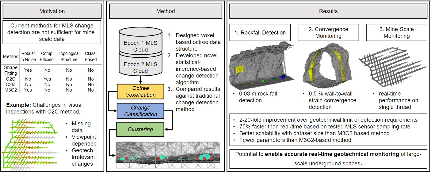
  • Design of a purpose-built voxel-based octree data structure for efficient processing of MLS point clouds and geotechnical metadata.
  • Development of a novel change detection algorithm that utilizes MLS-sensor-specific parameters to derive intra-voxel inference statistics to determine geotechnical risk and handle the low signal-to-noise ratio of MLS.
  • Comparison of our new framework using mine-wide MLS data collected with state-of-the-art SLAM-MLS against traditional change-detection methods, showing significantly improved computational performance for convergence and rockfall detection.

1.1. Traditional Deformation Analysis and Change Detection

Point cloud change detection and deformation analysis aim to classify and measure geometric differences between two co-registered scan epochs of the same scene [28]. Several studies have investigated deformation analysis methods in circular concrete-lined rail and highway tunnels. They primarily analyze static terrestrial laser scanning (TLS) data using mathematically parameterized geometric shapes like ellipses and rectellipses fitted to 2D cross-sections of point cloud data [7,29,30,31]. These global shape-fitting approaches do not perform optimally in mining environments for two main reasons: irregular drift shapes require relatively complex geometric models for parameterization, and irrelevant changes in the drift floor due to the addition or removal of material limit the amount of usable data [31]. These approaches are also not designed to identify discrete, localized failures such as roof fall and rib spalling [32]. While shape-fitting approaches have received attention in research, cloud-to-cloud (C2C) and cloud-to-mesh (C2M) have been some of the first to be employed for change detection in mining operations [33]. C2C provides fast computations but does not account for the directionality of change and is sensitive to point spacing and noise [34,35]. C2M distances, while providing directionally signed results, require computationally expensive meshing. C2M accuracy is also impacted by the quality of the mesh interpolation relative to the original surface [34]. Multi-scale model-to-model cloud comparison (M3C2) is a local averaging-based change detection method and does not require meshing as it operates directly on the point clouds. It calculates distances along a local normal vector estimated based on each point’s neighborhood of a specified size. M3C2 then projects search cylinders along the normal vectors and calculates the locally averaged change between the two input clouds [36]. M3C2 is the current state-of-the-art in geomorphic point cloud-based change analysis, especially for low-frequency TLS-based rock slope monitoring [37,38,39,40,41,42,43,44,45,46]. M3C2 and related methods have only seen limited use in the context of underground applications [31,47,48].
M3C2 change results can be used to identify statistically significant changes by estimating a “Level of Detection” [36], which is often underestimated on natural surfaces and, thereby, causes false negatives [35,44,49,50]. Winiwarter et al. [41] supplemented the M3C2 calculation with error propagation and covariance information. Their so-called M3C2-EP method demonstrates a lower level of detection than the original M3C2 implementation when tested on synthetic and field TLS data. Computational performance was not reported in the study. As M3C2-EP utilizes M3C2 with additional steps, its runtime is likely similar to, or higher than, M3C2. The M3C2-EP method requires additional metadata, such as sensor accuracy, alignment information, and scan positions. While M3C2 and its variants are more robust to noise than C2C and C2M, few studies have used it for mine-scale MLS-based change detection. Besides requiring extensive tuning for various data-sensor, application, and environment-dependent parameters, M3C2 and its variants’ main limitations for large-scale, complex, and mine-wide applications are their computational cost and resulting unsuitability for real-time processing.

1.2. Challenges in Large-Scale MLS Data Analysis

MLS point cloud data for monitoring are high in volume, frequency, and variety and can be defined as big data. These properties present challenges for conventional data processing methodologies [51], such as the ones for change detection summarized in Table 1. Our literature review presented studies that described their limitations regarding noise robustness and computational efficiency. In addition, we believe that their lack of topological structure and their natively non-classification-based change detection approach further limit their adoption for geotechnical monitoring.
C2C, C2M, and M3C2 results do not inherit 3D topological structures, such as information about spatially adjacent points. Instead, they output unstructured point cloud lists, similar to the input data format. The lack of topology makes the automation of 4D spatiotemporal analysis for underground convergence or rockfall challenging. Often time-consuming and error-prone visual interpretation is necessary to uncover regionally connected, time-dependent trends within the data. Additionally, the lack of topological structure makes traditional methods less compatible with advanced applications for autonomous mobile platforms that require topological information to perceive and navigate their environment [26]. Shape-fitting methods can provide some basic abstraction, e.g., by outputting results as individual cross-sections [7]. Spatial clustering can be a post-processing method that provides additional topological context and has been used for rockfall detection [44,52].
Current point cloud deformation and change detection analysis commonly evaluate change based on a calculated distance between point clouds from different epochs. This distance is often displayed as a continuous variable for individual points using a color scale and legend. While this is sufficient for low-frequency visual analysis of small scenes, it creates challenges for high-frequency, mine-scale monitoring. Some of these are exemplified and illustrated in Figure 1. Due to sensor noise, most points show 0.05 m of change, which likely marks the limit of detection. While filtering these points is trivial, other scenarios are more challenging to solve for easier interpretation. For example, in Figure 1A, points with distances larger than 0.2 m have been colored in grey to help identify missing data between two scan epochs. In Figure 1B, the transition from missing data to available data results in points incorrectly showing up to 20 cm changes. In Figure 1C, where partial coverage between two scans exists, distinguishing real changes from missing data is challenging. Viewing angle ambiguity is another challenge in visual interpretation, especially for large-scale and dense data. In Figure 1D, changes in the drift floor are only visible when data are viewed at an oblique angle and might be false positives, as Walton et al. [31] discussed. A high number of potential false positives in the dataset can obscure true positives in the mine drift roof in Figure 1E.
Visual interpretations are subjective, time-consuming, and error-prone and require manual steps to utilize results in business intelligence or automation workflows. For example, many mines utilize so-called Trigger Action Response Plans (TARPs) to manage geotechnical risks [53]. A TARP requires clearly defined alert levels based on real-time monitoring inputs or triggers, e.g., for a specific convergence rate. A classification-based change detection framework could incorporate mine-site-specific triggers and help eliminate delays and errors in the visual interpretation of monitoring data. A more automated, less subjective classification-based approach is desirable to improve the detection and differentiation of geotechnically relevant and significant changes.
Finally, a robust monitoring program must achieve a sufficient limit of detection. Critical convergence magnitudes with a potential negative impact on safety and productivity can be classified from 1–10%, i.e., 0.05 to 0.5 m of wall-to-wall convergence in a 5 m-wide drift [54]. Additionally, rockfall as small as 0.1 m in diameter has been shown to cause fatal injuries in underground mines [55]. For mine-wide monitoring of geotechnical hazards, we can assume that a practical limit of detection for convergence should at least be 0.05 m wall-to-wall change and 0.1 m edge-length for rockfall events.

1.3. Octree-Based Deformation Analysis and Change Detection

Several studies have undertaken underground deformation analysis using static lidar sensors. The previous section showed that MLS-based underground mine scale deformation and change detection provide opportunities to improve traditional approaches. As a core technology in robotic mapping [56], SLAM-based MLS [57], and point cloud data processing [34], voxel-based octree data structures could help solve the challenges traditional change detection methods face with mine-scale MLS data. An octree is a hierarchical data structure that divides 3D space into nodes [58,59]. Nodes are commonly represented by cubical volumes referred to as voxels. Each voxel can be recursively divided into eight smaller sub-sections until a minimum voxel size or tree depth is reached. The minimum voxel size l m i n determines the octree’s level of detail or resolution, with lower values representing higher resolutions. In robotic and laser-scanning applications, octree resolution is usually determined by available system memory, lidar sensor resolution, and application-specific requirements [56,60]. Additionally, lower resolutions of an octree can always be generated by performing cuts at any depth of the octree, making them multi-resolution. Lower octree resolution generally increases the speed of computational operations, such as tree-based searches [56]. In practice, l m i n can, therefore, be selected as small as memory availability allows but is usually limited by lidar data resolution and processing speed requirements.
In applications that utilize point cloud data from laser scanners, a voxel is usually initialized by integrating a laser-scan measurement with an x, y, and z location. In this basic form, a voxel encodes a simple Boolean property to describe the occupancy state of its space. Octrees can encode additional information, such as three-dimensional ellipsoids or surfel representations. These can be particularly interesting when processing low-precision MLS data, as they can encode statistical descriptors such as the mean, variance, and covariance of the points in each voxel. These statistics describe sampled surfaces in more detail than a Boolean occupancy property (Figure 2). Voxel and surfels have been used to improve SLAM performance with examples in indoor [61,62] and larger urban environments [63,64]. Zlot and Bosse [65] demonstrated the efficiency of ellipsoid-supplemented voxels for large-scale underground mine mapping but did not investigate multi-temporal applications such as ground movement monitoring.
Shortcomings of voxel-based representations include their susceptibility to discretization artifacts created when large, open scenes are not sufficiently observed and a loss in accuracy compared to the original point cloud data [66,67]. Underground mine environments present fewer discretization challenges due to their confined nature, high MLS sampling rates, and high point cloud density. The loss of accuracy remains a concern, especially in safety-critical monitoring applications. Gehrung et al. [68] address this in urban datasets by supplementing voxels with a local spatial data representation in the form of a three-dimensional Gaussian kernel. In a later version of their method, they detected the appearance and disappearance of objects like pedestrians and cars using a voxel edge length of 0.5 m [69]. Wellhausen et al. [70] presented a voxel-based change detection pipeline using distance computations, thresholding, clustering, and classification. Their approach detected objects larger than 0.5 m in real-time using a voxel edge length of 0.75 m. Gehrung et al.’s [69] and Wellhausen et al.’s [70] implementations of voxel-based change detection showed promising results in urban scenarios and for relatively high magnitudes of changes.
Previous voxel-based change detection work focused on relatively large and discrete changes in urban environments and often used high-accuracy lidar sensors. In contrast to these methods, our proposed approach for underground geotechnical monitoring must handle noisy MLS data and provide a low detection limit, preferably below the MLS sensor-specific range accuracy. Our approach must also accurately detect appearing objects characterized by high-magnitude changes in relatively small regions, such as the ones caused by rockfalls and low-magnitude, incremental deformation over larger regions associated with rockmass convergence. Unlike conventional change detection techniques employed in underground applications, our method needs to produce a robust binary change classification with user-definable risk tolerance and absolute magnitudes of changes. Lastly, we aim to develop a framework that can be utilized for various underground mining applications that require a highly efficient and customizable data storage and processing platform.

2. Materials and Methods

2.1. Octree and Statistical Inference-Based Change Detection Framework

Our approach automatically performs octree-based voxelization, change classification, and k-nearest-neighbor clustering (KNC) (Figure 3). When pre-collected lidar point cloud data are used, we initialize octree voxelization directly from .csv or other file types that can store x, y, and z coordinate values for Epoch 1 (E1) and Epoch 2 (E2) point clouds. We iterate over the list of points and insert them into the octree with a user-defined minimum voxel size l m i n . Our octree implementation is not limited by maximum depth, and its resolution is only limited by memory availability. During point insertion, we maintain summary statistics, including mean vector x and covariance matrix Σ of each voxel.
In contrast to C2C-, C2M-, and M3C2-based change detection, which rely on distance computations, we propose statistical inference-based change classification. Statistical hypothesis testing and confidence intervals consider the probability of an outcome based on the frequency of findings supporting this outcome. For underground mine monitoring, the outcome might be the occurrence of rockfall or convergence. The evidence can be derived from the distances between two point clouds over two or multiple epochs. A statistical test quantitatively assesses the probability of measured changes being significant versus being random. The Chi-Squared fit, or distribution, test checks whether a distribution of a sample corresponds to a predefined distribution [71,72]. The Chi-Squared fit test squares the difference between an observed ( x i ) and expected ( x E x p ) frequency and uses the sum of the resulting density function to accept or reject the null hypothesis H0 with the confidence level 1 α (level of significance) and the degree of freedom f = k 1 with k number of classes:
χ p 2 = i = 1 n x i x E x p 2 x E x p
H 0 : χ p 2 χ 1 α , k 1 2
The Chi-Squared test’s power increases with the number of samples, intuitively improving the test’s ability to discern actual changes from noise. Schiefer and Schiefer [71] suggest a minimum of n = 30 samples for Chi-Squared tests. Assuming a regular point spacing d, we estimate the octree resolution or minimum voxel edge length l m i n to capture at least n point pairs as:
l m i n d n 3 1
We consider l m i n as the theoretical threshold to achieve meaningful Chi-Squared results. In practice, larger voxels are often desirable as they are more computationally efficient and increase the power of our Chi-Squared test.
To adapt the Chi-Squared test to utilize mean and covariance, which we store for each voxel, we first compute x m e a n with the inverse of the covariance matrix Σ E 1 1 for a voxel in our reference epoch E1 and the inverse of the nearest neighboring voxel in our comparison E2 Σ E 2 1 and the mean vectors x E 1 and x E 2
x m e a n = Σ M e a n × ( Σ E 1 1 × x E 1 + Σ E 2 1 × x E 2 )
We then compute two chi-squared values χ E 1 and χ E 2 :
χ E 1 = x E 1 x m e a n [ Σ M e a n 1 × x E 1 x m e a n ]
χ E 2 = x E 2 x m e a n [ Σ M e a n 1 × x E 2 x m e a n ]
We compare the smallest Chi-Squared value to the three degrees of freedom Chi-Squared function at the typical α = 0.05 significance level. While this parameter resulted in good sensitivity and precision for our testing, different MLS and scenes might require further tuning. If H0 is rejected, the voxel is classified as a potential change candidate. We also calculate and report the Euclidean distance between each voxel’s mean in E1 and the mean of its nearest neighbor in E2:
d x E 1 , x E 2 = x E 1 , x x E 2 , x 2 + x E 1 , y x E 2 , y 2 + x E 1 , z x E 2 , z 2
The change candidate voxels are stored in a separate octree at the same resolution as the original octrees. This enables very efficient k-nearest-neighbor searches over the usually much smaller candidate space compared to the original octree. Potential change candidates are clustered using a k-nearest-neighbor approach to eliminate isolated candidates likely unrelated to semantically relevant changes. Implementing our octree in C++ facilitates efficient insertion, storage, and query operations to achieve desired computational performance.

2.2. Synthetic Datasets Generation

SDS1 is used to develop and test the deformation analysis capabilities of our framework (Figure 4). These are most relevant for tasks involving time-series monitoring of low-magnitude deformations such as rockmass convergence. We generated eight random sample epochs of SDS1 E1–E8, with 10,000 points each drawn from a population with standard deviation (SD) σ and mean x ¯ for their x, y, and z positions. To approximate the point distribution of an MLS output of a flat surface, the population SD σ x and σ y in x and y dimensions are set to 0.5 m and σ z 0.03 m in z-dimension. The population mean x ¯ x , x ¯ y , and x ¯ z values are set to 0 m for E1 and E2. In E3–E8, x ¯ z increases in 0.005 m increments to simulate a progressive change as expected for underground drift convergence. SDS2 simulates the appearance of a rock on a flat surface, such as a mine drift floor. SDS2 utilizes SDS1 E1 for its reference epoch. SDS2 E2 merges E1 with an additional 2500 points representing a 0.4 × 0.3 × 0.25 rock (A) without a synthetically applied SD.

2.3. Field Data Acquisition

We collected three field datasets (FDS) with two different MLSs (Figure 5). FDS1 and FDS2 were collected with an Emesent Hovermap [73]. FDS3 was collected with a Kaarta Stencil 2 [74] MLS provided by Mine Vision Systems. The Kaarta Stencil 2 uses a Velodyne VLP-16 Puck lidar scanner [75], a MEMS-based inertia measurement unit, and a grey-scale camera that was not activated during our tests because it is less reliable in irregularly lit underground conditions. The Stencil 2 can nominally collect 300,000 pts/s in single-return mode over a 360-degree horizontal field of view. The VLP-16 uses 16 channels, with an angular (vertical) resolution of 2.0 degrees and a uniform 30-degree vertical field of view. Velodyne reports an accuracy of ±0.03 m and a range of up to 100 m [75]. The Emesent Hovermap can be mounted on various mobile platforms and provides flight assistance and autonomous navigation capabilities to specific Uncrewed Aerial Vehicles (UAVs). It utilizes the same lidar sensor as the Karata Stencil 2 and a MEMS-based IMU. An action camera can be attached to colorize point clouds. Hovermap rotates the lidar sensor 360° along the long axis at a rate of 0.5 Hz resulting in a near 360° × 360° Field of View. Stencil 2 and Hovermap both utilize their respective proprietary SLAM solutions.
FDS1 and FDS2 were collected handheld at the Colorado School of Mines Edgar Experimental mine. FDS1 Version 1 E1 and E2 were collected in an underground mine drift before and after placing six rocks with edge lengths in different sizes ranging from 0.03 m to 0.35 m. The Hovermap was calibrated using its automated calibration process and scanning was conducted over an in-and-out trajectory with the Hovermap facing in the direction of travel. The ground truth labels for true positive changes are shown in color in Figure 5a(1–6). In FDS1 E2 V2, a 1 m 2 large area is transposed along the horizontal y-axis towards the drift center to simulate 0.01 m of rib convergence, shown in Figure 5a cluster 7. FDS2 E1 and E2 were collected in another section of the mine without introducing any physical changes. In FDS2 E2, we simulate 1 cm of radial convergence into the drift along the y-axis on both sides of the drift wall. The true positive labels are shown in Figure 5b(1,2). All grey points in Figure 5a,b are assigned to a true negative (unchanged) cluster. FDS3 E1 and E2 have been collected using a vehicle-mounted Kaarta Stencil 2 MLS at underground Mine-A, covering 5 km of drift at average driving speeds of 5 km/h. The epochs E1 and E2 have approximately 27-million points each. We split each dataset epoch into Sections I–IV of similar point count and matching spatial extent between the epochs for our runtime tests. Each section contains all points of the previous section, resulting in a progressively larger dataset, with Section IV containing all points.

2.4. Workflow and Parameter Selection

Figure 6 shows an overview of our test methodology applied to our synthetic and field data. The synthetic data were generated for deformation and object appearance testing and validation. We processed the field data collected with the Hovermap MLS using the Emesent Software (2022 version) [74]. We then co-registered, cropped, and aligned the epochs of each dataset with the cartesian coordinate axis in CloudCompare [76]. The Stencil 2 data were processed in the same way after pre-processing with Kaarta’s and Mine Vision Systems’ (2022 version) proprietary software. Each dataset is utilized for a specific test, including voxel size sensitivity, rockfall, combined rockfall and convergence detection, radial convergence detection, and runtime comparisons. Tests are performed using the M3C2-based and our voxel-based methods on a virtualized Ubuntu 18.05.06 running on an i9 processor and 6 GB RAM. For all tests, our approach is executed on a single thread.
M3C2 parameter selection is complex and should be adapted based on the application. This requires careful tuning of five main user-defined parameters, affecting distance calculation accuracy, reliability, and computational time [36]. For rockfall detection, the projection diameter is the most critical parameter. The user needs to consider point spacing, surface complexity and roughness, quality of data, and additional post-processing steps such as filtering and clustering when selecting it [44]. DiFrancesco et al. [44] showed that while the smallest projection diameter that consistently covers at least one point returns the highest true positive rates, it also significantly increases the false positive rates in complex terrain and rough surfaces.
For convergence detection with M3C2, the orientation of surface normals is critical for reliable distance calculation. Accurate normals are especially important for scenes like underground mine openings with large variations in roughness. While M3C2’s multi-scale normals can result in more accurate distances than fixed normals, they are also significantly slower to compute [36]. At a 0.5 m scale, our field data’s average point cloud roughness is 0.04 m, ranging from a low of 0.005 m for a flat drift floor to a high of 0.24 m for an exposed drift wall. This spread is three times larger than the one Lague et al. [36] reported in their study using multi-scale normals for TLS data of rock slopes, indicating that multi-scale normals should also be used for underground mining data. M3C2 performance can be improved by limiting the number of normal calculations to so-called “core points”, which effectively sub-sample the point cloud [36]. As the core point spacing also affects the orientation of the M3C2 normal vectors, its selection is correlated to computational performance and change detection and accuracy. In practice, it should be selected as low as possible but as high as necessary to maintain reasonable computation times. DiFrancesco et al. [44] chose a core point spacing representing their input data’s maximum point spacing. This approach cannot yield sufficient computational performance for our high-density, mine-scale data. To achieve better computational performance with M3C2, we had to increase the core point spacing to two times the input point cloud’s maximum spacing.
DiFrancesco et al. [44] show that M3C2-based rockfall detection accuracy can be improved with filtering and spatial density clustering steps. We apply a similar methodology using a 0.05 m limit of detection at 95% confidence representing two times the root mean square error of the point cloud-alignment process. To detect 0.01 m of convergence, we need to lower our threshold below the limit of detection to 0.01 m to achieve a true positive classification. We then remove noise and cluster points into labeled change objects within their bounding boxes using the connected components clustering (CCC) algorithm implemented in CloudCompare. CCC is computationally efficient and conceptually similar to DBSCAN and has been utilized for rockfall clustering [44,52]. We apply a volume-density filter (VDF) to remove lower-density clusters to reduce false-positive results further. The complete M3C2 approach applied in this study, including filtering and clustering steps, requires selecting up to 12 parameters.
For our method, four parameters need to be selected, with octree resolution defined by the minimum voxel size l m i n being the most important. For our high-density data, voxel sizes between 0.1 m and 0.25 m, which exceed the minimum edge length l m i n by a factor of 10 to 25, have shown good change detection performance. These larger voxels also significantly improve the power of the Chi-Squared test, as voxels capture between 20–100 times more than are recommended for a strong Chi-Squared test. For the lower-density FDS3, we found that exceeding the estimated minimum voxel edge length by about 2.5 times with 0.25 m voxels works well, capturing around 200 points per voxel. Through testing, we determined that a confidence level of 0.05 and a minimum KNC size of two voxels results in optimal results for our data. All parameters for each test for the M3C2-based approach and ours are summarized in Table A1. We evaluate the change detection accuracy of both approaches for all datasets and discuss their implications for underground monitoring.
We test the real-time processing capabilities and dataset size scalability of M3C2 and our approach on our mine-scale dataset FDS3 Set I–IV. Based on the sampling rates of MLS, like the ones used to collect our data, we consider processing speeds higher than 300,000 pts/s as real-time capable. We test all M3C2 parameter combinations used for the rockfall and convergence detection tests in FDS1 and FDS2. We do not report the time required for either method for pre-processing, co-registration, cropping, and alignment steps. For the M3C2-based method, we only report M3C2-distance computations due to the extensive time required for manual threshold filtering, CCC, and VDF steps. For our approach, we report the total computation time for all steps.

3. Results and Discussion

3.1. Proof of Concept

We utilized the two synthetic datasets SDS1-2 for iterative development and testing and to derive initial parameters for real-world data. The theoretical limit of detection of our approach was assessed with SDS1. We selected a minimum voxel size l m i n of 5.0 m that encompasses all points in a single voxel. Results in Figure 7 show that the Chi-Squared Cumulative Density Function (CDF)-value generated by our solution correlates well with changes in the z-mean value and Euclidian distance. We can observe an exponential increase in the Chi-Squared metric as the standard deviation of our point cloud at 0.03 m is approached. With a significance level of α = 0.05, the first true-positive change detection occurs at 0.026 cm z-mean delta between E1 and E8. The results of our tests with SDS1 prove the conceptual functionality of our solution. The progressive one-dimensional translation in SDS1 is comparable to the expected changes in MLS data caused by the convergence in underground mine drifts.
We also tested the functionality of our approach for appearing objects. Figure 8 compares conventional cloud-to-cloud (C2C) distance computation to the output of our approach for SDS2 that simulates MLS data before and after a rockfall event. Based on the evaluation of field data and to ensure sufficient points per voxel, we selected a 0.5 m voxel size. We adapted the color scale to achieve the maximum true-positive classification of the C2C method. This approach results in a significant number of points being misclassified as changed (teal). In contrast, our approach proves to handle appearing objects while robust to the noisy input data with no false-positive change classification. Figure 8 also showcases the effect of two different voxel sizes on the resulting resolution of the computed covariance ellipsoids. We can observe that both voxel scales and respective ellipsoids in (1) give a good representation of the floor. Smaller voxels generate more detailed ellipsoid representations of their contained surfaces. This phenomenon can be observed in the ellipsoid configuration around the rock (2).

3.2. Voxel Size Sensitivity Tests

Table 2 and Figure 9 shows the change detection results for FDS1 Version 1 for five different voxel sizes from 0.1 m to 1.0 m. We also compared the effect of KNC filtering versus the unfiltered data. Our approach detects all rocks at l m i n of 0.1 m (A), including the smallest 0.03 m × 0.10 m × 0.05 m rock. At this minimum octree resolution, multiple voxels encompass each rock, with points of the smallest rock split between two voxels. No false negatives occur as we use KNC with a minimum cluster size of two. Increasing l m i n to 0.15 m (B) causes a false negative on the smallest rock, while the others are still correctly identified. The false negative is caused by KNC using a minimum cluster size of two and removing the single voxel in which the rock is detected. The same behavior is observed for l m i n of 0.25 m size (C). At l m i n of 0.5 m (D), only the largest rocks are encompassed by more than one voxel. This results in false negatives when applying the KNC filter to Rocks 4, 5, and 6. They are correctly classified in our unfiltered results. At l m i n of 1.0 m (E), only the largest rock is correctly identified in our unfiltered data. We find that l m i n up to approximately eight times the change target’s size appears most sensitive. For higher octree resolutions, enforcing a minimum sample size and using a KNC filter effectively prevents and removes false positives.

3.3. Change Detection Accuracy Tests

Table 3 and Figure 10 show the results and output clusters of M3C2 and our method with and without filtering using CCC (M3C2) and KNC (ours) for FDS1 (a–c) and FDS2 (d). Figure 10a shows the unfiltered outputs of M3C2 and ours for FDS1 V1. We can observe that significant noise remains before applying CCC. Irregular point scattering in the original cloud can result from water reflections, unfavorable incidence angles, and varying viewpoints during different MLS epochs. In complex underground mine drift scenes, open boreholes in drift walls (A), cables and pipes (B), and other irregular objects (C) can create challenges in generating a “clean” point cloud when collecting data. Compared to the M3C2 results obtained using a 95% confidence level threshold filter, our approach achieves significantly fewer false positives in regions with high point scatter (A, B, C).
Figure 11 illustrates how we effectively suppress noise within our approach without additional KNC. Our covariance-supplemented voxels produce less noise as they can better represent high-roughness surfaces. M3C2 generates noise around complex geometries that are challenging to capture with MLS due to the variations in viewpoints and additional scatter. An example is a wooden beam shown in Figure 10a (C) or the cables and pipes on the mine roof (B).
As the M3C2-distance of target No. 6 is smaller than the threshold filter value, all its points are removed, causing a false negative. As shown in Figure 10b, CCC removes all but 15 false positive clusters, which can be removed using VDF in the last step of the M3C2 method. Our method correctly detects all six rocks as true positive changes without creating false positives. Using an l m i n of 0.1 m, our approach returns the four changes voxels that encompass the smallest rock No. 6, showing good performance even if objects span multiple voxels. While we could detect target No. 6 with M3C2 when applying a higher confidence level and lower limit of detection threshold, the noise increases, which results in a higher potential for false positive results after CCC and VDF steps.
Using FDS1 V2, we tested M3C2s and our approach’s ability to detect both types of changes, rockfall and convergence, in the same scene. The results are shown in Figure 10c. For the M3C2-based approach to extract the 0.01 m of convergence, we must lower the M3C2-distance filter threshold to 0.01 m. This change also allows M3C2 to detect all six rockfalls. As expected, the lower threshold filter value creates noisier results than those obtained using the 0.05 m filter threshold. In total, M3C2 with CCC generates 28 false positive clusters. The point density withing these false positive clusters is high, resulting in similar densities as the true positive change clusters of rocks. In FDS1 V1, point clusters representing rockfalls can be separated from noise based on their higher volumetric density. The lowest-density rock cluster has a 20% higher density than the highest-density noise cluster. As we showed for FDS1 V1 in Figure 10b, additional filtering using VDF is critical to remove all remaining false positive clusters generated by CCC. However, this approach is not feasible for FDS1 V2 when convergence and rockfalls occur in the same dataset. Low-magnitude convergence clusters show a larger spatial extent than rockfalls while approximating 2D surfaces, resulting in a lower volumetric point density within each cluster. The convergence cluster has a 10% lower volume density than the highest noise cluster in our example. This would require a decision to either balance a higher false-positive rate when using a lower density cutoff with higher false-negative rates when choosing a higher density cutoff. Both options would compromise the applicability of M3C2 change detection and VDF for underground space monitoring.
In contrast, our approach detects all rocks and convergence without false-positive results in FDS1 V2. It is also worth pointing out that our approach measures the convergence distances with a mean deviation of less than 0.5 mm from the ground truth distance of 0.01 m, while M3C2 distances show a deviation of 1 mm from the ground truth. This represents a 0.5 mm absolute, or 100% relative, improvement in distance computation accuracy. M3C2’s lower accuracy is likely due to its dependence on correct surface normal orientations, which are known to be sensitive to datasets with high surface roughness [36].
With FDS2, we tested the detection of radial convergence of 0.01 m within a 4.3 m-diameter drift representing 0.02 m or 0.5% of wall-to-wall strain. Figure 10d shows that our approach can detect the 0.01 m convergence on each rib without any false positives when utilizing 0.25 m voxels. M3C2 generates 163 false-positive clusters using the same CCC settings as our previous tests. While a 20-times increase in the minimum points per component for CCC from 30 to 600 removes all false positives, it would limit the ability to detect smaller-scale convergence and rockfall with M3C2. Similar to FDS1 V2, if rockfall monitoring was required, VDF cannot be applied effectively as the noise is highly localized and dense. We observe more noise and false positive clusters in FDS2 than in FDS1. Most false positive clusters are located in the roof and lower drift walls with high surface roughness, indicating a similar issue as in FDS1 V1, where unfavorable incidence angles create excessive noise. The persistent challenge of noise, large variations in surface roughness, and resulting inconsistencies in M3C2 surface normal estimation in MLS data likely contribute to the weak change detection performance of M3C2 in complex underground scenes.
Based on all tests, we find that a voxel size of 0.25 m enables the detection of rockfalls as small as 0.03 m and convergence as low as 0.01 m. Our current implementation of KNC filtering provides higher sensitivity with smaller voxel sizes and improves our approach’s precision. Our approach achieves a 2-to-20-times lower detection limit than geotechnical monitoring requirements based on our literature review. M3C2 and density-based clustering methods like CCC and VDF are sensitive to variations between the tested types of changes in two datasets, making them less generalizable and suitable for mine-scale monitoring of convergence and rockfall. While the M3C2-based approach generally provides similar sensitivity to ours, its precision is much lower, especially without additional clustering and filtering steps.

3.4. Runtime Comparison

We test the computational performance of our framework and the M3C2-method using FDS3. As the use of core points and multi-scale surface normals in M3C2 significantly affects its runtime, we evaluated all four combinations of Parameter Settings 1–4. We also compared ours to the single-thread performance of M3C2. The methods are shown in Table 4.
Table 5 summarizes the results of a runtime comparison using M3C2 and our approach on the mine-scale dataset FDS3. As the performance of M3C2 S1 and S2 for the smallest Section I was already significantly lower than the real-time threshold of 300,000 pts/s, larger dataset versions were not tested. M3C2 S3 shows slightly higher than real-time performance for Sections I and II, but performance drops below 300,000 pts/s for Sections III and IV. Due to the lack of multi-scale normal computations, S3 should also not be used when high-accuracy convergence detection is required. S4 is equivalent to the settings we used for our tests in FDS1 and FDS2 to achieve optimal change detection accuracy for M3C2, but it fails to deliver real-time performance by a significant margin. As expected, S5 and S6, which are equivalent to S3 and S4 but executed on a single thread, cannot deliver real-time performance. Our method delivers higher than real-time change detection with 75–82% performance margins for all tested dataset sizes. It also shows the lowest performance drop with dataset size increase of all tested methods. When comparing against the M3C2 settings S4 and S6 that delivered the best change detection results for M3C2 in our tests with FDS1, our method achieves 15 and 50 times better computational performance compared to multi- and single-threaded M3C2 while delivering on-par, or better, change detection results. Our method’s single-threaded performance surpasses the fastest M3C2 settings executed on eight threads, S3, by a factor of 1.8. It is also important to note that the core point spacing parameter for M3C2 was set to 0.1 m, which is twice as high as the point cloud spacing and, therefore, at the upper limit to achieve reasonable change detection performance as defined by DiFrancesco et al. [44]. Similar to increasing our minimum voxel size to 0.25 m, which achieved good change detection performance, increasing core point spacing can improve computational performance at the cost of lower change detection sensitivity. As our method achieves significantly higher than real-time performance using a single CPU thread, integration on modern MLS using multi-core CPUs is conceivable. It is also worth noting that a significant reduction of computational overhead can be achieved by integrating our framework into MLS or robotic mapping software, which commonly uses octree data structures [77,78].

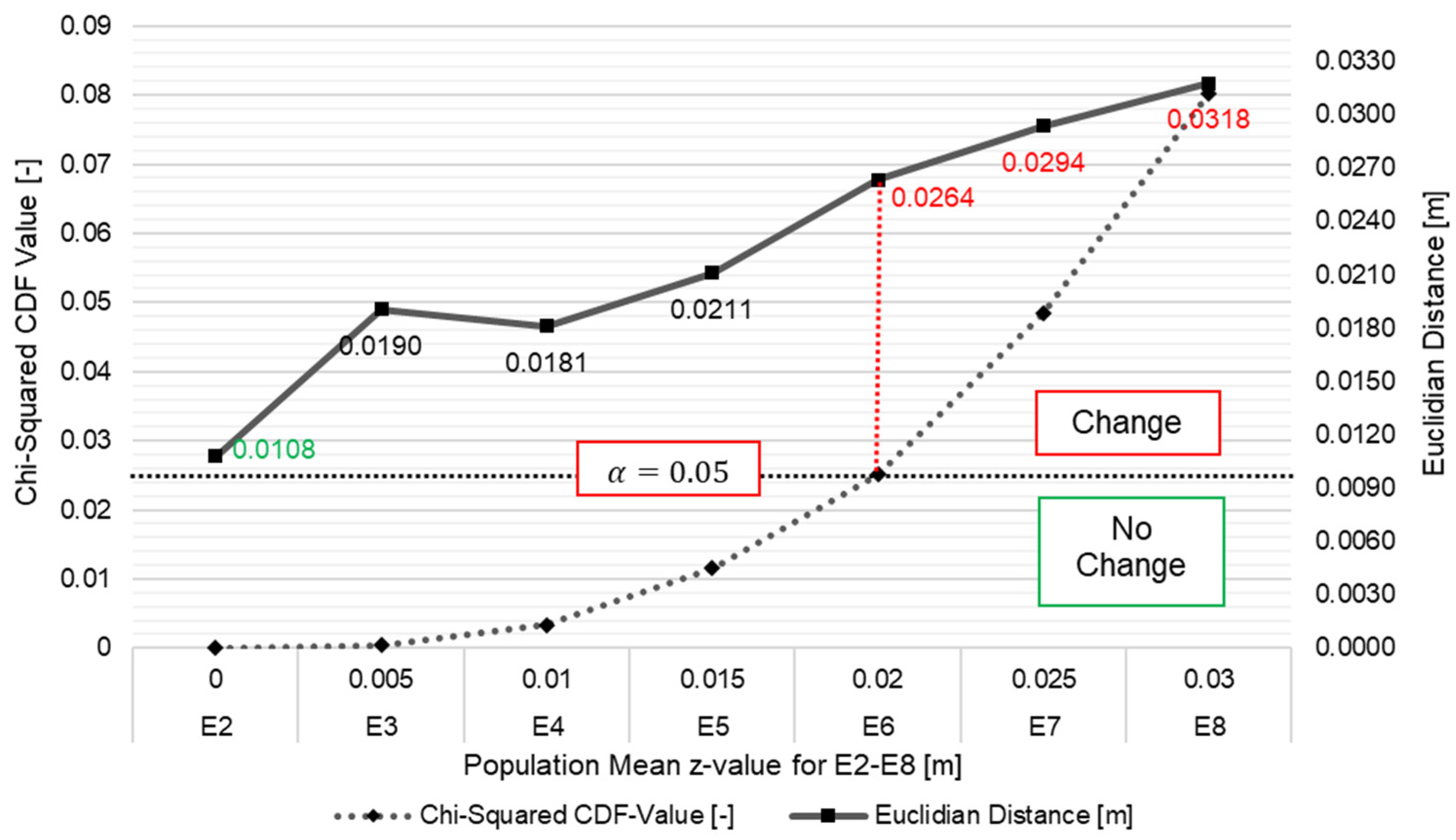
3.5. Discussion of p-Value-Based Decision-Making

Our method relies on the p-value-based classification of changes. There is an ongoing debate within the scientific community about the applicability, correct use, and meaningfulness of p values in statistical inference testing [79,80,81,82]. The main concerns are interpretation, reproducibility, and the practical importance of “significant” findings derived from statistical analysis utilizing the p-value.
Nuzzo [79] points out that p-values are often misinterpreted and were intended as an “informal way to judge whether the evidence was significant in the old-fashioned sense: worthy of a second look”. Similarly, Wasserstein and Lazar [81] emphasize that small p values “[…] can be interpreted as casting doubt on or providing evidence against the null hypothesis or the underlying assumptions”, and they advise that “scientific conclusions and business or policy decisions should not be based only on whether a p-value passes a specific threshold." Both statements highlight the potential of p values to be misused as binary, isolated, and definitive classifiers for the results’ (in)significance. While we were able to validate the quality of our results with ground truth data, we recognize the current limitations of implying p values as our primary indicator for change. In an operational scenario, where pragmatic safety- and business-relevant decisions must be made, relying on p values alone is not advisable. Many statisticians advocate for Bayesian statistics as one possible solution [79,80,81,82]. The Bayesian framework uses prior knowledge and tracks changes in probabilities of outcomes as new evidence arises. This approach is intuitively compelling for underground change detection as prior knowledge is often available. While a Bayesian approach could provide an alternative to frequentist results, it still requires a definition of a change–classification threshold. Multi-method approaches are another solution to reduce reliance on p values [79] and could be a potential avenue for future research. While p-values have limitations, we see them as a valuable tool to robustly identify regions of change and aid geotechnical engineers in prioritizing further inspections.

3.6. Additional Benefits of an Octree-Based Framework

Large-scale MLS data processing is often only feasible after significant down sampling, i.e., the deletion of valuable and expensive information. While the lidar sensors used in current MLS samples are about 300,000 points per second, future MLSs will offer much higher sampling rates. Other compact lidar sensors can already sample over 2.5-million points per second [83]. This increase in data will also require more efficient processing methods that can utilize this additional information without first reducing it. Our approach offers significant computational performance benefits over traditional change detection methodologies and is more scalable to larger datasets than M3C2, which arguably represents the best currently available alternative algorithm for underground change detection from point clouds.
The performance improvement of our voxel-based approach is significant despite it not yet being optimized or parallelized. A graphics processing unit (GPU)-based parallelization of voxel-based data structures is a promising avenue for further improvements of our method. Hoezlein [84] developed a highly parallelized GPU voxel database structure (GVDB) with simulation and visualization applications. Both are highly relevant for monitoring and other geotechnical tasks, such as numerical modeling. Min et al. [85] showed significant performance improvements using GPU ray tracing for volumetric mapping. Although implemented in our approach, we currently do not utilize ray tracing. In a future version of our method, we might use ray tracing to reduce false–positive rates for dynamic object removal and occlusion handling [86].
Xu et al. [67] highlight the benefits of voxels for classifying large point cloud datasets. For example, Wang et al. [87] have shown the efficacy of an octree-based convolutional neural network for 3D shape analysis and classification. Point cloud segmentation and classification are highly relevant for underground monitoring and digital-twin applications. Segmentation and classification contextualize data, enabling advanced filters, visualizations, and computations. Classifying a mine drift’s roof, wall, and floor in conjunction with detected changes would help better understand convergence behavior. Voxel-based data structures and spatial representations also have great potential for global-scale digital-twin models, autonomous robotic, and internet-of-things applications [88,89]. So far, their efficiency and flexibility have not been adequately explored for underground mining applications.

4. Conclusions

This paper presents a novel, octree-based data processing and change detection framework that can handle noisy point cloud data and perform statistical inference-based change detection using enhanced voxels. Our method provides a binary classification of changes and absolute magnitudes of deformations in a topologically connected octree data structure. Our approach identifies changes that are 66% below the lidar sensor-specific range accuracy of 0.03 m and detects rockfall events with side lengths as small as 0.03 m and convergence as low as 0.01 m or 0.5% wall-to-wall strain. Compared to the current limit of detection requirements in geotechnical monitoring applications, this represents a three-fold improvement for rockfall and a 2–20-fold improvement for convergence detection.
In comparison to the state-of-the-art M3C2-based approach, our method detects all six targets without false positives, while M3C2 misses the smallest target. Our statistical inference-based approach handles noisy data better and produces fewer false positives than M3C2. In single-pass rockfall and convergence detection scenarios, where M3C2’s volume density-based filtering is inapplicable, our method outperforms M3C2 as its clusters cannot be effectively removed. Our approach is less sensitive to parameter selection and provides superior distance calculation accuracy, especially in areas of high-surface roughness.
On a mine-scale dataset, our approach achieves these results at a performance that is 75% faster than real-time, while none of the six tested M3C2 settings achieve real-time performance. Our method’s single-threaded performance is 15 times higher than M3C2 executed on eight threads and 50 times higher than single-threaded M3C2. Our method also achieves more than four times better computational performance scalability with dataset size. We achieve these results with only four paraments, a third of the parameters required for the M3C2-based method. Therefore, our method requires less tuning and can achieve higher generalizability.
Additional benefits of our approach include a more automated workflow and the ability to store other data within its efficient octree-data structure. Together, these improvements are a significant step towards adopting MLS data for geotechnical hazard monitoring for large-scale underground caverns, tunnels, and mines. Future work will focus on testing the framework on larger datasets and enhancing change detection accuracy by incorporating geotechnically relevant metadata.

Author Contributions

Conceptualization, L.F. and A.J.P.; Methodology, L.F.; Software, L.F. and A.J.P.; Formal Analysis, L.F.; Resources, L.F., A.J.P. and G.W.; Data Curation, L.F.; Writing—Original Draft Preparation, L.F.; Writing—Review & Editing, L.F., A.J.P., G.W., E.A.H. and J.F.B.; Funding Acquisition, E.A.H., G.W. and A.J.P. All authors have read and agreed to the published version of the manuscript.

Funding

This work was supported in part by the Alpha Foundation for the Improvement of Mine Safety and Health, Inc. [AFC820-54]; and by the National Institute of Occupational Safety and Health (NIOSH) [200-2016-90154].

Data Availability Statement

3rd-Party Data. Restrictions apply to the availability of Field Dataset (FDS) 3. Data were obtained from an undisclosed third party and are available from the authors with the permission of third party. Other data are available on request from the corresponding author.

Acknowledgments

We want to acknowledge the staff at Mine-A and Lee Fronapfel and Clinton Dattel at the Edgar Experimental Mine, who enabled and supported our fieldwork. We would also like to acknowledge the support of instrumentation partner Emesent for providing their Hovermap MLS and Mine Vision Systems for their Kaarta Stencil 2. We also thank Scott Schiele and Pete Carney of Mine Vision Systems, and Stefan Hrabar (Emesent) for valuable discussions and technical advice. We appreciate the comments provided by three reviewers to improve the quality of this manuscript.

Conflicts of Interest

The authors declare no conflict of interest.

Appendix A

Table A1. Summary of processing parameter by test and dataset for M3C2-based, as well as our own, workflows.
UnitFDS1 V1FDS1 V2FDS2FDS3
Dataset Properties
Test Focus-RockfallRockfall & ConvergenceRadial ConvergenceRuntime
Instrument-HovermapHovermapHovermapStencil 2
Points per EpochM3.33.32.25–27
Raw Data Point Spacingm0.0050.0050.0050.05
Mean Roughness-0.040.040.040.13
M3C2-Based Method
M3C2 Distance Computations
Normal Calculation MethodmFixedMulti-ScaleMulti-ScaleBoth
Core Point Spacingm0.010.010.010.1
Fixed Normal Diameterm1.0--3.25
Minimum Normal Diameterm-0.1250.1250.125
Step Normal Diameterm-0.20.20.2
Max Normal Diameterm-6.1256.1256.125
Projection Diameterm0.030.030.030.3
Maximum Projection Depthm0.50.50.50.5
Threshold Filtering
Limit of Detectionm0.050.010.01-
Clustering
CCC Octree Depth-888-
CCC Minimum Points-303030-
Volume Density Filtering
Points per Cubic Meterpts/m350k35k35k-
Ours
Octree Voxelization
Voxel Sizem0.10.10.250.25
Change Classification
Min Points per Voxel - 50505050
Significance Level - 0.050.050.050.05
KNC
Minimum Cluster Size - 2222

References

  1. Terzaghi, K. Shield tunnels of the Chicago Subway. J. Boston Soc. Civ. Eng. 1942, 29, 163–210. [Google Scholar]
  2. Ma, K.; Zhang, J.; Zhou, Z.; Xu, N. Comprehensive analysis of the surrounding rock mass stability in the underground caverns of Jinping I hydropower station in Southwest China. Tunn. Undergr. Space Technol. 2020, 104, 103525. [Google Scholar] [CrossRef]
  3. Hu, Z.; Wu, B.; Xu, N.; Wang, K. Effects of discontinuities on stress redistribution and rock failure: A case of underground caverns. Tunn. Undergr. Space Technol. 2022, 127, 104583. [Google Scholar] [CrossRef]
  4. Li, S.; Yu, H.; Liu, Y.; Wu, F. Results from in-situ monitoring of displacement, bolt load, and disturbed zone of a powerhouse cavern during excavation process. Int. J. Rock Mech. Min. Sci. 2008, 45, 1519–1525. [Google Scholar] [CrossRef]
  5. Zhao, J.S.; Jiang, Q.; Lu, J.F.; Chen, B.R.; Pei, S.F.; Wang, Z.L. Rock fracturing observation based on microseismic monitoring and borehole imaging: In situ investigation in a large underground cavern under high geostress. Tunn. Undergr. Space Technol. 2022, 126, 104549. [Google Scholar] [CrossRef]
  6. Wittke, W.; Pierau, B.; Erichsen, C. New Austrian Tunneling Method (NATM)—Stability Analysis and Design; WBI: Essen, Germany, 2006. [Google Scholar]
  7. Walton, G.; Delaloye, D.; Diederichs, M.S. Development of an elliptical fitting algorithm to improve change detection capabilities with applications for deformation monitoring in circular tunnels and shafts. Tunn. Undergr. Space Technol. 2014, 43, 336–349. [Google Scholar] [CrossRef]
  8. Kaiser, P.K.; Cai, M. Design of rock support system under rockburst condition. J. Rock Mech. Geotech. Eng. 2012, 4, 215–227. [Google Scholar] [CrossRef] [Green Version]
  9. Mark, C.; Molinda, G.M. Preventing falls of ground in coal mines with exceptionally low-strength roof: Two case studies. In Proceedings of the 23rd International Conference on Ground Control in Mining, Morgantown, WV, USA, 3–5 August 2004. [Google Scholar]
  10. Nordlund, E. Deep hard rock mining and rock mechanics challenges. In Proceedings of the Ground Support 2013: The Seventh International Symposium on Ground Support in Mining and Underground Construction, Perth, Australia, 13 May 2013; pp. 39–56. [Google Scholar] [CrossRef] [Green Version]
  11. Oraee, K.; Oraee, N.; Goodarzi, A.; Khajehpour, P. Effect of discontinuities characteristics on coal mine stability and sustainability: A rock fall prediction approach. Int. J. Min. Sci. Technol. 2016, 26, 65–70. [Google Scholar] [CrossRef] [Green Version]
  12. Palei, S.K.; Das, S.K. Sensitivity analysis of support safety factor for predicting the effects of contributing parameters on roof falls in underground coal mines. Int. J. Coal Geol. 2008, 75, 241–247. [Google Scholar] [CrossRef]
  13. Sandbak, L.A.; Rai, A.R. Ground Support Strategies at the Turquoise Ridge Joint Venture, Nevada. Rock Mech. Rock Eng. 2013, 46, 437–454. [Google Scholar] [CrossRef]
  14. Centers for Disease Control and Prevention. NIOSH Mine and Mine Worker Charts. 2021. Available online: https://wwwn.cdc.gov/niosh-mining/MMWC (accessed on 2 September 2021).
  15. Williams, K.; Olsen, M.J.; Roe, G.; Glennie, C. Synthesis of transportation applications of mobile LiDAR. Remote Sens. 2013, 5, 4652–4692. [Google Scholar] [CrossRef] [Green Version]
  16. Luo, X.; Ren, X.T.; Li, Y.; Wang, J.J. Mobile surveying system for road assets monitoring and management. In Proceedings of the 2012 7th IEEE Conference on Industrial Electronics and Applications (ICIEA), Singapore, 18–20 July 2012; pp. 1688–1693. [Google Scholar]
  17. Puente, I.; Akinci, B.; González-Jorge, H.; Díaz-Vilariño, L.; Arias, P. A semi-automated method for extracting vertical clearance and cross sections in tunnels using mobile LiDAR data. Tunn. Undergr. Space Technol. 2016, 59, 48–54. [Google Scholar] [CrossRef]
  18. Raval, S.; Banerjee, B.P.; Singh, S.K.; Canbulat, I. A Preliminary Investigation of Mobile Mapping Technology for Underground Mining. In Proceedings of the IGARSS 2019–2019 IEEE International Geoscience and Remote Sensing Symposium, Yokohama, Japan, 28 July–2 August 2019; pp. 6071–6074. [Google Scholar]
  19. Lynch, B.K.; Marr, J.; Marshall, J.A.; Greenspan, M. Mobile LiDAR-Based Convergence Detection in Underground Tunnel Environments. 2017. Available online: http://hdl.handle.net/1974/15638 (accessed on 17 May 2022).
  20. Singh, S.K.; Banerjee, B.P.; Raval, S. A review of laser scanning for geological and geotechnical applications in underground mining. Int. J. Min. Sci. Technol. 2023, 33, 133–154. [Google Scholar] [CrossRef]
  21. Fahle, L.; Holley, E.; Walton, G. Toward a mine-wide, real-time, and autonomous geotechnical change detection, monitoring, and prediction framework for underground mines. In Proceedings of the 39th International Conference on Ground Control in Mining, ICGCM 2020, Canonsburg, PA, USA, 28–30 July 2020. [Google Scholar]
  22. Fahle, L.; Holley, E.A.; Walton, G.; Petruska, A.J.; Brune, J.F. Analysis of SLAM-Based Lidar Data Quality Metrics for Geotechnical Underground Monitoring. Min. Metall. Explor. 2022, 39, 1939–1960. [Google Scholar] [CrossRef]
  23. Gallwey, J.; Eyre, M.; Coggan, J. A machine learning approach for the detection of supporting rock bolts from laser scan data in an underground mine. Tunn. Undergr. Space Technol. 2021, 107, 103656. [Google Scholar] [CrossRef]
  24. Watson, C.; Marshall, J. Estimating underground mine ventilation friction factors from low density 3D data acquired by a moving LiDAR. Int. J. Min. Sci. Technol. 2018, 28, 657–662. [Google Scholar] [CrossRef]
  25. Engin, I.C.; Maerz, N.H.; Boyko, K.J.; Reals, R. Practical Measurement of Size Distribution of Blasted Rocks Using LiDAR Scan Data. Rock Mech. Rock Eng. 2020, 53, 4653–4671. [Google Scholar] [CrossRef]
  26. Marshall, J.; Barfoot, T.; Larsson, J. Autonomous underground tramming for center-articulated vehicles. J. Field Robot. 2008, 25, 400–421. [Google Scholar] [CrossRef]
  27. Jones, E.; Ghabraie, B.; Beck, D. A method for determining field accuracy of mobile scanning devices for geomechanics applications. In Proceedings of the ISRM International Symposium—10th Asian Rock Mechanics Symposium, ARMS 2018, Singapore, 29 October–3 November 2018; pp. 978–981. [Google Scholar]
  28. Lindenbergh, R.; Pietrzyk, P. Change detection and deformation analysis using static and mobile laser scanning. Appl. Geomat. 2015, 7, 65–74. [Google Scholar] [CrossRef]
  29. Wannenmacher, H.; Krenn, H.; Komma, N.; Tunnel, A.S. Improved pressure tunnel lining methods, a case study of the Niagara Tunnel Facility Project. In World Tunnel Congress 2013, Geneva; Anagnostou, G., Ehrbar, H., Eds.; CRC Press: London, UK, 2013. [Google Scholar]
  30. Nuttens, T.; Stal, C.; de Backer, H.; Schotte, K.; van Bogaert, P.; de Wulf, A. Methodology for the ovalization monitoring of newly built circular train tunnels based on laser scanning: Liefkenshoek Rail Link (Belgium). Autom. Constr. 2014, 43, 1–9. [Google Scholar] [CrossRef]
  31. Walton, G.; Diederichs, M.S.; Weinhardt, K.; Delaloye, D.; Lato, M.J.; Punkkinen, A. Change detection in drill and blast tunnels from point cloud data. Int. J. Rock Mech. Min. Sci. 2018, 105, 172–181. [Google Scholar] [CrossRef]
  32. Han, J.Y.; Guo, J.; Jiang, Y.S. Monitoring tunnel deformations by means of multi-epoch dispersed 3D LiDAR point clouds: An improved approach. Tunn. Undergr. Space Technol. 2013, 38, 385–389. [Google Scholar] [CrossRef]
  33. Fekete, S.; Diederichs, M.; Lato, M. Geotechnical and operational applications for 3-dimensional laser scanning in drill and blast tunnels. Tunn. Undergr. Space Technol. 2010, 25, 614–628. [Google Scholar] [CrossRef]
  34. Girardeau-Montaut, D.; Roux, M.; Marc, R.; Thibault, G. Change Detection on Points Cloud Data Acquired with A Ground Laser Scanner. In Proceedings of the ISPRS WG III/3, III/4, V/3 Workshop “Laser Scanning 2005”, Enschede, The Netherlands, 12–14 September 2005. [Google Scholar]
  35. Barnhart, T.B.; Crosby, B.T. Comparing two methods of surface change detection on an evolving thermokarst using high-temporal-frequency terrestrial laser scanning, Selawik River, Alaska. Remote Sens. 2013, 5, 2813–2837. [Google Scholar] [CrossRef] [Green Version]
  36. Lague, D.; Brodu, N.; Leroux, J. Accurate 3D comparison of complex topography with terrestrial laser scanner: Application to the Rangitikei canyon (N-Z). ISPRS J. Photogramm. Remote Sens. 2013, 82, 10–26. [Google Scholar] [CrossRef] [Green Version]
  37. Williams, J.G.; Rosser, N.J.; Hardy, R.J.; Brain, M.J.; Afana, A.A. Optimising 4-D surface change detection: An approach for capturing rockfall magnitude-frequency. Earth Surf. Dyn. 2018, 6, 101–119. [Google Scholar] [CrossRef] [Green Version]
  38. van Veen, M.; Hutchinson, D.J.; Kromer, R.; Lato, M.; Edwards, T. Effects of sampling interval on the frequency—magnitude relationship of rockfalls detected from terrestrial laser scanning using semi-automated methods. Landslides 2017, 14, 1579–1592. [Google Scholar] [CrossRef]
  39. Kromer, R.A.; Abellán, A.; Hutchinson, D.J.; Lato, M.; Edwards, T.; Jaboyedoff, M. A 4D filtering and calibration technique for small-scale point cloud change detection with a terrestrial laser scanner. Remote Sens. 2015, 7, 13029–13058. [Google Scholar] [CrossRef] [Green Version]
  40. Bonneau, D.A.; Hutchinson, D.J. The use of terrestrial laser scanning for the characterization of a cliff-talus system in the Thompson River Valley, British Columbia, Canada. Geomorphology 2019, 327, 598–609. [Google Scholar] [CrossRef]
  41. Winiwarter, L.; Anders, K.; Höfle, B. M3C2-EP: Pushing the limits of 3D topographic point cloud change detection by error propagation. ISPRS J. Photogramm. Remote Sens. 2021, 178, 240–258. [Google Scholar] [CrossRef]
  42. Abellán, A.; Jaboyedoff, M.; Oppikofer, T.; Vilaplana, J.M. Detection of millimetric deformation using a terrestrial laser scanner: Experiment and application to a rockfall event. Nat. Hazards Earth Syst. Sci. 2009, 9, 365–372. [Google Scholar] [CrossRef] [Green Version]
  43. Abellán, A.; Oppikofer, T.; Jaboyedoff, M.; Rosser, N.J.; Lim, M.; Lato, M.J. Terrestrial laser scanning of rock slope instabilities. Earth Surf. Process. Landf. 2014, 39, 80–97. [Google Scholar] [CrossRef]
  44. DiFrancesco, P.M.; Bonneau, D.; Hutchinson, D.J. The implications of M3C2 projection diameter on 3D semi-automated rockfall extraction from sequential terrestrial laser scanning point clouds. Remote Sens. 2020, 12, 1885. [Google Scholar] [CrossRef]
  45. Kromer, R.A.; Hutchinson, D.J.; Lato, M.J.; Gauthier, D.; Edwards, T. Identifying rock slope failure precursors using LiDAR for transportation corridor hazard management. Eng. Geol. 2015, 195, 93–103. [Google Scholar] [CrossRef]
  46. Lato, M.J.; Diederichs, M.S.; Hutchinson, D.J.; Harrap, R. Evaluating roadside rockmasses for rockfall hazards using LiDAR data: Optimizing data collection and processing protocols. Nat. Hazards 2012, 60, 831–864. [Google Scholar] [CrossRef]
  47. Evans, P. Improving Convergence Monitoring Using Lidar Data At Rio Tinto’S Argyle Diamond Mine Improving Convergence Monitoring Using Lidar Data at Rio Tinto’S Argyle Diamond Mine. 2021, pp. 1–12. Available online: https://www.emesent.io/2021/05/26/improving-convergence-monitoring-using-lidar-data-at-rio-tintos-argyle-diamond-mine/ (accessed on 21 March 2023).
  48. Vanneschi, C.; Mastrorocco, G.; Salvini, R. Assessment of a rock pillar failure by using change detection analysis and FEM modelling. ISPRS Int. J. Geo-Inf. 2021, 10, 774. [Google Scholar] [CrossRef]
  49. Benjamin, J.; Rosser, N.; Brain, M. Rockfall detection and volumetric characterisation using LiDAR. In Landslides and Engineered Slopes. Experience, Theory and Practice; CRC Press: Boca Raton, FL, USA, 2016; Volume 2, pp. 389–395. [Google Scholar] [CrossRef]
  50. Ozdogan, M.V.; Deliormanli, A.H. Landslide detection and characterization using terrestrial 3D laser scanning (LIDAR). Acta Geodyn. Geomater. 2019, 16, 379–392. [Google Scholar] [CrossRef] [Green Version]
  51. Gandomi, A.; Haider, M. Beyond the hype: Big data concepts, methods, and analytics. Int. J. Inf. Manag. 2015, 35, 137–144. [Google Scholar] [CrossRef] [Green Version]
  52. Tonini, M.; Abellan, A. Rockfall detection from terrestrial lidar point clouds: A clustering approach using R. J. Spat. Inf. Sci. 2014, 8, 95–110. [Google Scholar] [CrossRef]
  53. Sharon, R.; Eberhardt, E. Guidelines for Slope Performance Monitoring; CSIRO Publishing: Collingwood, Australia, 2020. [Google Scholar] [CrossRef]
  54. Mercier-Langevin, F.; Hadjigeorgiou, J. Towards a better understanding of squeezing potential in hard rock mines. Min. Technol. 2011, 120, 36–44. [Google Scholar] [CrossRef]
  55. Mark, C.; Iannacchione, A.T. Best Practices to mitigate injuries and fatalities from rock falls. In Proceedings of the 31st Annual Institute on Mining Health, Safety and Research, Roanoke, Virginia, 27–30 August 2000; pp. 115–129. Available online: https://stacks.cdc.gov/view/cdc/8586 (accessed on 14 August 2022).
  56. Hornung, A.; Wurm, K.M.; Bennewitz, M.; Stachniss, C.; Burgard, W. OctoMap: An efficient probabilistic 3D mapping framework based on octrees. Auton. Robot. 2013, 34, 189–206. [Google Scholar] [CrossRef] [Green Version]
  57. Zhang, J.; Singh, S. Low-drift and real-time lidar odometry and mapping. Auton. Robot. 2017, 41, 401–416. [Google Scholar] [CrossRef]
  58. Wilhelms, J.; van Gelder, A. Octrees for faster isosurface generation. ACM Trans. Graph. 1992, 11, 201–227. [Google Scholar] [CrossRef]
  59. Meagher, D. Geometric modeling using octree encoding. Comput. Graph. Image Process. 1982, 19, 129–147. [Google Scholar] [CrossRef]
  60. Berrio, J.S.; Zhou, W.; Ward, J.; Worrall, S.; Nebot, E. Octree map based on sparse point cloud and heuristic probability distribution for labeled images. In Proceedings of the 2018 IEEE/RSJ International Conference on Intelligent Robots and Systems (IROS), Madrid, Spain, 1–5 October 2018. [Google Scholar] [CrossRef]
  61. Park, C.; Moghadam, P.; Kim, S.; Elfes, A.; Fookes, C.; Sridharan, S. Elastic LiDAR Fusion: Dense Map-Centric Continuous-Time SLAM. In Proceedings of the IEEE International Conference on Robotics and Automation, Brisbane, Australia, 21–25 May 2018. [Google Scholar] [CrossRef] [Green Version]
  62. Whelan, T.; Leutenegger, S.; Salas-Moreno, R.F.; Glocker, B.; Davison, A.J. ElasticFusion: Dense SLAM without a pose graph. Robot. Sci. Syst. 2015, 11, 1–9. [Google Scholar] [CrossRef]
  63. Behley, J.; Stachniss, C. Efficient Surfel-Based SLAM using 3D Laser Range Data in Urban Environments. Robot. Sci. Syst. XIV 2018, 2018, 59. [Google Scholar] [CrossRef]
  64. Droeschel, D.; Behnke, S. Efficient continuous-time SLAM for 3D lidar-based online mapping. In Proceedings of the 2018 IEEE International Conference on Robotics and Automation (ICRA), Brisbane, Australia, 21–25 May 2018; pp. 5000–5007. [Google Scholar] [CrossRef] [Green Version]
  65. Zlot, R.; Bosse, M. Efficient Large-Scale 3D Mobile Mapping and Surface Reconstruction of an Underground Mine; Springer Tracts in Advanced Robotics: Heidelberg, Germany, 2014; Volume 92, pp. 479–494. [Google Scholar] [CrossRef]
  66. Gehrung, J.; Hebel, M.; Arens, M.; Stilla, U. A Voxel-Based Metadata Structure for Change Detection in Point Clouds of Large-Scale Urban Areas. ISPRS Ann. Photogramm. Remote Sens. Spat. Inf. Sci. 2018, 4, 97–104. [Google Scholar] [CrossRef] [Green Version]
  67. Xu, Y.; Tong, X.; Stilla, U. Voxel-based representation of 3D point clouds: Methods, applications, and its potential use in the construction industry. In Automation in Construction; Elsevier B.V.: Amsterdam, The Netherlands, 2021; Volume 126. [Google Scholar] [CrossRef]
  68. Gehrung, J.; Hebel, M.; Arens, M.; Stilla, U. A fast voxel-based indicator for change detection using low resolution octrees. ISPRS Ann. Photogramm. Remote Sens. Spat. Inf. Sci. 2019, 4, 357–364. [Google Scholar] [CrossRef] [Green Version]
  69. Gehrung, J.; Hebel, M.; Arens, M.; Stilla, U. Change Detection and Deformation Analysis Based on Mobile Laser Scanning Data of Urban Areas. ISPRS Ann. Photogramm. Remote Sens. Spat. Inf. Sci. 2020, 5, 703–710. [Google Scholar] [CrossRef]
  70. Wellhausen, L.; Dube, R.; Gawel, A.; Siegwart, R.; Cadena, C. Reliable real-time change detection and mapping for 3D LiDARs. In Proceedings of the SSRR 2017—15th IEEE International Symposium on Safety, Security and Rescue Robotics, Shanghai, China, 11–13 October 2017; pp. 81–87. [Google Scholar] [CrossRef] [Green Version]
  71. Schiefer, H.; Schiefer, F. Statistics for Engineers; Springer Fachmedien Wiesbaden: Wiesbaden, Germany, 2021. [Google Scholar] [CrossRef]
  72. Pearson, K. X. On the criterion that a given system of deviations from the probable in the case of a correlated system of variables is such that it can be reasonably supposed to have arisen from random sampling. Lond. Edinb. Dublin Philos. Mag. J. Sci. 1900, 50, 157–175. [Google Scholar] [CrossRef] [Green Version]
  73. Emesent. Hovermap. 2022. Available online: https://www.emesent.com/hovermap/ (accessed on 15 August 2022).
  74. Kaarta. Kaarta Products. 2022. Available online: https://www.kaarta.com/products/stencil-2-for-rapid-long-range-mobile-mapping/ (accessed on 21 March 2023).
  75. Velodyne LiDAR. Velodyne LiDAR ‘Puck’ LITE Light Weight Real-Time 3D LiDAR Sensor: Product Specification. 2022. Available online: https://velodynelidar.com/products/puck-lite/ (accessed on 21 March 2023).
  76. CloudCompare. CloudCompare. 2021. Available online: https://www.danielgm.net/cc/ (accessed on 21 March 2023).
  77. Park, C.; Kim, S.; Moghadam, P.; Fookes, C.; Sridharan, S. Probabilistic Surfel Fusion for Dense LiDAR Mapping. In Proceedings of the 2017 IEEE International Conference on Computer Vision Workshops, ICCVW 2017, Venice, Italy, 22–29 October 2017. [Google Scholar] [CrossRef] [Green Version]
  78. Trăsnea, B.; Ginerică, C.; Zaha, M.; Măceşanu, G.; Pozna, C.; Grigorescu, S. Octopath: An octree-based self-supervised learning approach to local trajectory planning for mobile robots. Sensors 2021, 21, 3606. [Google Scholar] [CrossRef] [PubMed]
  79. Nuzzo, R. Statistical Errors. Nature 2014, 506, 150–152. [Google Scholar] [CrossRef] [PubMed] [Green Version]
  80. Baker, M. Statisticians issue warning on P values. Nature 2016, 531, 151. [Google Scholar] [CrossRef] [Green Version]
  81. Wasserstein, R.L.; Lazar, N.A. The ASA’s Statement on p-Values: Context, Process, and Purpose. In American Statistician; American Statistical Association: Boston, MA, USA, 2016; Volume 70, pp. 129–133. [Google Scholar] [CrossRef] [Green Version]
  82. Siegfried, T. Odds Are, It’s Wrong. Available online: https://www.sciencenews.org/article/odds-are-its-wrong (accessed on 12 March 2010).
  83. Ouster. ULTRA-WIDE VIEW LIDAR SENSOR OS0. 2021. Available online: https://ouster.com/products/os0-lidar-sensor/ (accessed on 21 March 2023).
  84. Hoetzlein, R.K. GVDB: Raytracing sparse voxel database structures on the GPU. In Proceedings of the High-Performance Graphics—ACM SIGGRAPH/Eurographics Symposium Proceedings, HPG, Dublin, Ireland, 20–22 June 2016; Volume 2016. [Google Scholar] [CrossRef]
  85. Min, H.; Han, K.M.; Kim, Y.J. Accelerating Probabilistic Volumetric Mapping using Ray-Tracing Graphics Hardware. In Proceedings of the 2021 IEEE International Conference on Robotics and Automation (ICRA), Xi’an, China, 30 May–5 June 2021. [Google Scholar] [CrossRef]
  86. Underwood, J.P.; Gillsjo, D.; Bailey, T.; Vlaskine, V. Explicit 3D change detection using ray-tracing in spherical coordinates. In Proceedings of the IEEE International Conference on Robotics and Automation, Karlsruhe, Germany, 6–10 May 2013; pp. 4735–4741. [Google Scholar] [CrossRef] [Green Version]
  87. Wang, P.S.; Liu, Y.; Guo, Y.X.; Sun, C.Y.; Tong, X. O-CNN: Octree-based convolutional neural networks for 3D shape analysis. ACM Trans. Graph. 2017, 36, 1–11. [Google Scholar] [CrossRef] [Green Version]
  88. Sennersten, C.; Davie, A.; Lindley, C. Voxelnet—An Agent Based System for Spatial Data Analytics. In Proceedings of the COGNITIVE: The Eigth International Conference on Advanced Cognitive Technologies and Applications, Rome, Italy, 20–24 March 2016; pp. 133–136. [Google Scholar]
  89. Sennersten, C.; Lindley, C.; Evans, B. VoxelNET’s Geo-Located Spatio Temporal Softbots. In Proceedings of the COGNITIVE: The Eigth International Conference on Advanced Cognitive Technologies and Applications, Venice, Italy, 5–9 May 2019; pp. 20–27. [Google Scholar]
Figure 1. Example of color-coded lidar data of mine-wide changes by absolute distances. (A): Missing data, (B): Transition from missing data to available data, (C): Partial coverage between two scans, (D): Changes in drift floor, (E): Potential false positives in drift roof.
Remotesensing 15 01764 g001
Figure 2. Schematic of a volumetric (a) and tree (b) representation of an octree structure storing Boolean occupancy free (white) and occupied (grey). Example of an occupied voxel of size lmin storing MLS points of a surface (c), a graphical representation of the covariance of the points (d), and the data maintained in our octree (e).
Remotesensing 15 01764 g002
Figure 3. Schematic overview of our octree voxelization, statistical inference-based change detection, and KNC framework showing input parameters, use of octrees, and processing steps.
Remotesensing 15 01764 g003
Figure 4. Overview of SDS1 E1-4 inside a schematic voxel (a) and SDS2 (b).
Remotesensing 15 01764 g004
Figure 5. Overview of FDS 1–3 (ac) with true positive (changed) in color and true negative (unchanged) in grey. FSD3 with progressively larger sections I–IV.
Remotesensing 15 01764 g005
Figure 6. Flowchart of our study methodology for SDS1-2 and FDS1-3.
Remotesensing 15 01764 g006
Figure 7. Results of the SDS1 test showing the exponential increase of the Chi-Squared CDF-value vs. the linearly increasing Euclidean distance.
Remotesensing 15 01764 g007
Figure 8. Plan and section views of SDS2 E1 and E2 with a 0.4 × 0.3 × 0.25 rock appearing in E2 and 0.5 m voxels for C2C and our approach (a). Top-down and side view of SDS2 and voxel-ellipsoid representation based on 0.5 m (brown) and 0.3 m (grey) minimum voxel size (b). Both lmin values create good ellipsoid representations of the floor (1). Smaller voxels generate more detailed ellipsoid representations of rock (2).
Remotesensing 15 01764 g008
Figure 9. Results of rockfall and voxel size test in FDS1 V1 with six progressively smaller rocks (1–6) from edge lengths from 0.25–0.03 m. Comparison of results for voxel sizes (A: 0.1 m, B: 0.15 m, C: 0.25 m, D: 0.5 m, E: 1.0 m).
Remotesensing 15 01764 g009
Figure 10. Change detection results of M3C2 workflow and ours on FDS1 and FDS2. (a) M3C2 without any filtering (no CCC/VDF) showing rockfall targets 1–6 and noisy M3C2 output (A–C). (b) M3C2 only with CCC, VDF can remove all shown false negative clusters showing rockfall target 1–6. (c) M3C2 with CCC, VDF cannot be applied showing rockfall targets 1–6 and convergence target 7. (d) M3C2 with CCC showing convergence targets 1–2 and increased noise in the floor (A) and roof (B).
Remotesensing 15 01764 g010
Figure 11. A close-up view of Region C in Figure 10a showing covariance per voxel as green and red ellipsoids for Epochs 1 and 2, respectively. Meshing also performs poorly on the wooden beam (B). M3C2 produces false positives around the wooden beam (A) and rock bolts (D) due to unfavorable incidence angles and occlusion. A good fit of covariance ellipsoids to the beam’s flat surface and the rough surface of the drift wall (C) can be observed. A good match between E1 and E2 ellipsoids results in a low false-positive rate.
Remotesensing 15 01764 g011
Table 1. Properties of traditional change detection methods.
MethodRobust to NoiseComputationally EfficientTopological StructureClassification-BasedReferences
Shape FittingYesNoNoNo[7,29,30,31]
C2CNoYesNoNo[34,35]
C2MNoNoNoNo[34]
M3C2YesNoNoNo[36]
Table 2. Results of voxel-size sensitivity tests.
IDVoxel Size [m]Detected TargetsComment
KNCNo Filter
A0.106/66/6-
B0.155/66/6KNC removes target cluster (No. 6) with <2 voxels
C0.252/66/6KNC removes target clusters No. 3–6 with <2 voxels
D0.502/64/6KNC removes target clusters No. 4–6 and No. 2 with <2 voxels
E1.000/61/6Only target No. 1 is correctly classified in unfiltered data
Table 3. Number of targets detected by M3C2 and our method.
DatasetM3C2 (CCC)Ours (KNC)M3C2 Comment
FDS1 V15/66/6One false negative (Target No. 6) caused by threshold filtering
Fifteen false positive noise clusters remain after CCC
FDS1 V27/77/7Twenty-eight false positive clusters caused by 0.01 m threshold filter
VDF not applicable
FDS22/22/2One hundred sixty-three false positive clusters remain after CCC
Table 4. Tested M3C2 setting for core point and multi-scale normals.
SettingCore PointsMulti-Scale NormalsThreads
S1FalseFalse8
S2FalseTrue8
S3TrueFalse8
S4TrueTrue8
S5TrueFalse1
S6TrueTrue1
Table 5. Processing speed in points per second for M3C2 Method S1-6 and ours for FDS3 Section I–IV.
FDS3 Section
M3C2 SettingI
5.4 M Pts/Epoch
II
10.9 M Pts/Epoch
III
18.7 M Pts/Epoch
IV
27.7 Pts/Epoch
Change from I to IV
S125.32DNCDNCDNC-
S21.22DNCDNCDNC
S3318.67321.46297.20297.97−6%
S433.2430.0328.8129.48−11%
S5137.85139.95120.80114.75−17%
S610.75DNCDNCDNC-
Ours546.39546.13534.29524.88−4%
Real-Time Margin82%82%78%75%
DNC: Did not complete.
Disclaimer/Publisher’s Note: The statements, opinions and data contained in all publications are solely those of the individual author(s) and contributor(s) and not of MDPI and/or the editor(s). MDPI and/or the editor(s) disclaim responsibility for any injury to people or property resulting from any ideas, methods, instructions or products referred to in the content.

