Range-Doppler Based Moving Target Image Trace Analysis Method in Circular SAR

Abstract

The single channel Circular Synthetic Aperture Radar (CSAR) has the advantage of continuous surveillance of a fixed scene of interest, which can provide high frame rate image sequences to detect ground moving targets. Recent image-sequence-based CSAR moving target detection methods utilize the fact that the target signal moves fast in the image sequence. Knowledge of the target’s image trace(moving trace in the image sequence, which is equal to a target signature’s morphology in a full aperture CSAR image) can help design better detection methods. However, previous signature morphology studies are based on linear track geometry assumptions, which cannot handle CSAR’s nonlinear track. Hence, this paper proposes a new image trace method based on the range-Doppler principle. The proposed method can deduct the exact analytic function of an arbitrary moving target’s image trace in CSAR. The method assumes radar operates in side-looking mode and that the target moves on the ground plane. It combines the range-Doppler equations(i.e., iso-range and iso-Doppler relation) and Cartesian transformation between the ground and radar coordinate system to obtain the parametric functions of the image trace. Based on the method, three types of target motion (including linear and nonlinear motion) are analyzed. The proposed method is validated with both simulated and real data.

1. Introduction

Ground Moving Target Indication (GMTI) is a hot topic in Synthetic Aperture Radar (SAR) research. Because of its all-day and all-weather capabilities, numerous research outcomes have been applied to traffic monitoring and military applications.

Current studies are based on the assumption that radar flies in a linear trajectory. Raney first studied moving target signatures. He noted that delocalization is caused by range speed, and the defocusing effect is caused by range acceleration and azimuth speed [1]. Based on the analysis in [1], two main processing categories have been developed. One category is multichannel techniques such as ATI, DPCA, and STAP [2,3,4]. Although these techniques have good performance in moving target detection and motion parameter estimation, they require complex hardware. The second category is based on single-channel systems, which is still a significant research topic. Related methods, such as [1,5,6], mainly utilized defocusing and delocalization characteristics to perform detection and motion parameter estimations. However, those traditional single channel methods suffer from several disadvantages such as requiring high PRF and relatively long processing time due to the iteration processes. These disadvantages limit GMTI performance in conventional linear track SAR (linear SAR). Recent studies have revealed that Circular Synthetic Aperture Radar (CSAR) can detect moving targets with only subaperture image sequences, thereby mitigating the above problem.

CSAR is a new imaging mode that has been developed since the 90s [7,8,9]. Unlike typical linear SAR and LEO (Low Earth Orbit) SAR, CSAR can provide ultra-high resolution due to its full aspect data acquiring capability. Although it was first successfully applied in airborne platforms, it currently also serves as the validation tool for research on Geosynchronous SAR [10,11]. Geosynchronous SAR has an ‘8’ shaped trajectory, which makes it possible to acquire full aspect data in space scenarios such as CSAR. In GMTI applications, CSAR has advantages that include the following. First, its long time observation (typically several minutes or more) feature is good for target detection and tracking [12], which is very good for applications such as city traffic monitoring. Second, its circular geometry makes it possible to record a target’s Doppler information from ${360}^{\circ }$, which is good for velocity estimation and relocation [13]. The typical detection method utilizes the target signature’s complex motion on an image sequence. Such complexly shaped traces on an image sequence (denoted as image traces for short) are caused by a circular trajectory. One example is shown in Figure 1: a linearly moving target generates a ‘V’ shaped signature in CSAR imagery. By comparison, the same target motion generates simple hyperbolic or elliptic shape in conventional linear SAR [14].

To develop better methods such as detection or speed estimation, this requires more knowledge on a target’s signature. In [13], Poisson et al. deduced the signal model of a target’s signature and proposed an algorithm to reconstruct a moving target’s real trace by using its image trace. However, such modeling can only give numerical results and cannot deduce analytic expressions. Our team proposed a single-channel CSAR moving target detection algorithm that is entitled logarithm background subtraction [12]. This method utilizes the characteristics of a target complex image trace to detect moving targets with subaperture image sequences. The above methods take advantage of the moving target’s new feature in CSAR. Thus, to further understand CSAR’s potential and limits in GMTI, the analysis of moving target image traces in CSAR imagery is necessary.

Prior image trace studies have focused on linear SAR. Researchers have investigated the moving target’s image trace in linear SAR imagery by using mathematical deduction and numerical computation. In [14], Jen King Jao deduced the constant speed of a moving target’s image trace function in linear SAR, which proved that this kind of target image trace was in a hyperbolic shape. Reference [15] used numerical simulation to analyze other moving target types’s image traces in linear SAR images; the effects of changes in target speed and heading direction were also discussed. In [16], Garren, D.A. proposed a method for linear SAR to obtain an image trace’s analytical functions based on serial expansion. Later, based on this method, he discussed the squint angle’s influence on the image trace in linear SAR [17,18]. By using an image trace function, reference [19] discussed the moving target detection ambiguity problem in linear SAR. Since the curved geometry in CSAR is more complex than linear SAR, the investigation on mathematical expressions of moving target’s signature requires a new method.

In this paper, a method of deducing an image trace’s mathematical formulas is proposed. The ground coordinate and radar coordinate system are used. The proposed method combines the range-Doppler equations and Cartesian coordinate system transformation to obtain the parametric functions of the moving target’s image trace. It first uses the ground-to-radar coordinate system transformation to obtain the target’s instantaneous speed and position in the radar coordinate system. Next, the range-Doppler equations are solved to get its image position. Finally, the image trace functions in the original ground coordinate system are obtained using radar-to-ground coordinate system transformation. The method can handle targets with arbitrary motion forms. The following three types of moving target’s parametric functions are then analyzed:

Type A:

constant speed

Type B:

constant acceleration

Type C:

rotating around a scene center with a constant speed

The effectiveness is demonstrated by simulated and real SAR data.

The paper is organized as follows. Section 2 describes the material and dataset used in this paper. Section 3 describes the detail of the image trace formulation method. Section 4 gives examples, and corresponding point target simulations are presented to validate the method. Section 5 details an experiment with real data. Section 6 pertains to the discussion. Section 7 finishes with the conclusion.

2. Material and Dataset

The data used in this paper has two parts: the simulated circular SAR raw data and the real data of the GOTCHA dataset.

2.1. Simulated Data

The SAR system works in side-looking mode. The radar’s parameters for the simulation are shown in

Table 1. SAR Simulation Parameters.

Symbol	SAR Parameters	Value
$f_c$	Center frequency	9.6 GHz
$B_d$	Bandwidth	640 MHz
$PRF$	Pulse repetition frequency	1.32 kHz
$R_0$	Ground range to scene center	3000 m
${\theta }_{inc}$	Incidence angle	${45}^{\circ }$
$v_s$	Radar speed	200 m/s
${\theta }_{azi}$	Azimuth integration angle	${180}^{\circ }$ (90°~−90°)

. The echo can be simulated with no approximation according to [20]. Here, the radar moves clockwise. Because circular SAR geometry is symmetrical, and full aspect data require a long time for processing, the integrated aperture is set to ${180}^{\circ }\left([{90}^{\circ },-{90}^{\circ }]\right)$. Consider the algorithm designed to get the moving target image trace on the ground plane rather than the slant plane. The Back-Projection (BP) imaging algorithm was selected to generate the SAR images for the following examples. The BP algorithm is an accurate time-domain SAR imaging algorithm that is typically applied to circular SAR data processing [20]. As for other imaging algorithms, such as the Chirp Scaling (CS) algorithm, the slant plane images from different apertures should project onto the uniform ground plane image grid through an interpolation process.

2.2. Real Data

The GOTCHA dataset is an open-access airborne CSAR dataset published by the airforce research laboratory [21]. The purpose of publishing these data is to provide sources of research for moving target detection, refocusing, and tracking application. Since then, various research have been published using the GOTCHA dataset [22,23,24,25,26,27,28]. Along with SAR data, the ground truth of a moving vehicle (i.e., its speed and trajectory information) is provided. Thus, we can compute its image trace and verify it with the generated CSAR image. We first introduce the related information for computing the corresponding image trace. Then, we conduct an analysis on a small scene to show method result.

The top view of the platform and the target’s relative motion are shown in Figure 2. The platform trace is plotted with a dashed line, and the moving target trace is plotted with a solid line. Their moving directions are indicated by arrows. The coordinate system is the Processor Coordinate System (PCS) attached to the data. The radar moves clockwise with an average speed of 110 m/s and a mean height of 7251 m. The average radius is 7266 m. The illumination time is 71 s. During the observation, the moving vehicle first travels away from an intersection. Then, it accelerates in the negative direction of the PCS-X axis. Finally, the car turns toward the positive direction of the PCS-Y axis after deceleration.

3. Image Trace Formulation Method

A straightforward method to obtain analytic expression for a target’s image trace is solving the range-Doppler Equations (range-Doppler here defines iso-range and iso-Doppler relations, rather than the SAR imaging algorithm) in one Cartesian coordinate system. This works for the linear SAR case, since the radar moving direction does not change. If using the along-track and across-track directions to build the coordinate system, the across-track components of the radar velocity and position term become zero. Therefore, the complexity of the range-Doppler equations can be reduced. However, CSAR’s circular trajectory has two velocity components. Thus, the complexity of the range-Doppler equations cannot be reduced, which makes equations difficult to solve. Consider two facts: (1) the range-Doppler equations can easily solve for each instantaneous radar coordinate system (i.e., using the along-track and across-track directions to build the system in each azimuth time); (2) the parametric functions that we want are expressed in the Cartesian ground coordinate system. Thus, the proposed method introduces a coordinate system transformation and combines the range-Doppler equations to deduce the analytic expressions of the image trace.

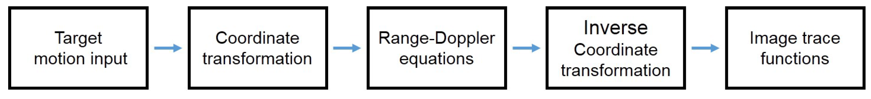
A flowchart is shown in Figure 3. The input target’s motion parameters are its position and velocity expressed in the ground coordinate system. The method uses the ground-to-radar transformation to obtain the target’s instantaneous speed and position in the radar coordinate system. In the radar coordinate system, the radar-related vectors have a simple form. Thus, the complexity of the range-Doppler equations can be reduced. Then, we can write down the image trace functions in the radar coordinate system. The analytic expressions of the image trace in the ground coordinate system are then obtained via inverse transformation.

3.1. Step 1: Transformation

It is assumed that radar flies in a circular trajectory with in side-looking mode, and the target moves on the ground plane. The ideal PRF is assumed so that target-motion-induced Doppler ambiguity can be neglected. Consider the use of two coordinate systems, where the symbol ‘˜’ denotes variables in the radar coordinate system. For deduction convenience, the label ‘$\left(t\right)$’ for all time-varying variables, such as the target position and velocity, is omitted.

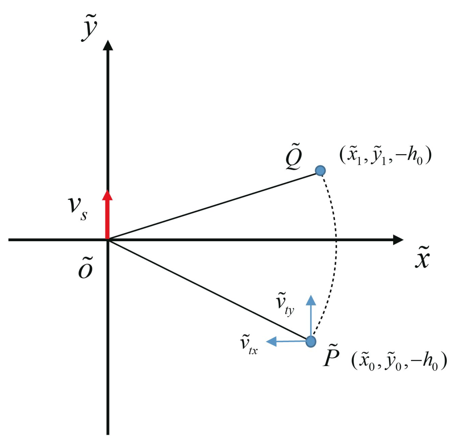
The top view of the geometry is shown in Figure 4. $XOY$ is the ground coordinate system, and O is the scene center. Then, the set radar moves clockwise as the positive direction. For a ${360}^{\circ }$ aperture, the radar’s start point lies on the negative side of the X axis. When the time $t=0$, the radar lies on the positive side of the X axis. The radar moves with a constant speed $v_s$ at height $H_0$. The radius of the circle is $R_0$. At time $t_0$, a moving target is located at $P:(x_0,y_0,0)$ with velocity vector ${\overrightarrow{v}}_t:(v_{tx},v_{ty},0)$. When the radar lies on $\tilde{O}$, the angle between $O\tilde{O}$ and the positive part of the X axis is $\alpha =-\frac{v_{s}t}{R_0}={\omega }_{s}t$ (${\omega }_s$ is the radar’s angular velocity). We set $\tilde{O}$ as the origin, and $\tilde{X}\tilde{O}\tilde{Y}$ is the instantaneous radar coordinate system. $\overrightarrow{O\tilde{O}}$ is the $\tilde{X}$ axis, and the radar moving direction is the $\tilde{Y}$ axis.

$\tilde{P}:({\tilde{x}}_0,{\tilde{y}}_0,0)$ and ${\overrightarrow{\tilde{v}}}_t:({\tilde{v}}_{tx},{\tilde{v}}_{ty},0)$ are the target’s position and velocity in the transformed system, respectively. Then, the coordinate system transformation of the input target’s parameters from $XOY$ to $\tilde{X}\tilde{O}\tilde{Y}$ is given by

$$\begin{array}{c}\hfill \left\{\begin{array}{cc}\hfill {\tilde{x}}_0& =R_0-x_{0}cos\alpha -y_{0}sin\alpha \hfill \\ \hfill {\tilde{y}}_0& =x_{0}sin\alpha -y_{0}cos\alpha \hfill \\ \hfill {\tilde{z}}_0& =-H_0\hfill \\ \hfill {\tilde{v}}_{tx}& =-v_{tx}cos\alpha -v_{ty}sin\alpha \hfill \\ \hfill {\tilde{v}}_{ty}& =v_{tx}sin\alpha -v_{ty}cos\alpha \hfill \end{array}\right.\end{array}$$

(1)

In (1), the ${\tilde{v}}_{tx}$ and ${\tilde{v}}_{ty}$ were obtained by coordinate system transformation with a fixed azimuth angle $\alpha ={\omega }_{s}t$ in instantaneous time t. From the physics point of view, if the reader wants to calculate ${\tilde{v}}_{tx}$ and ${\tilde{v}}_{ty}$ by the derivative of ${\tilde{x}}_0$ and ${\tilde{y}}_0$, the term with $cos\alpha =cos{\omega }_{s}t$ and $sin\alpha =sin{\omega }_{s}t$ should be treated as constant. Another conclusion in (1) was that the transformation of Z is a constant, as the radar and target have no motion along the Z axis. It will be shown in the next subsection that height $H_0$ does not play a role in the deduction because of this reason.

3.2. Step 2: Solution of Range-Doppler Equation

The range-Doppler equations are the basic principles of SAR imaging. We obtained analytic expressions of the moving target image position by solving such equations in the radar coordinate system. The top view of the $\tilde{X}\tilde{O}\tilde{Y}$ system is shown in Figure 5. $\tilde{P}$ and $\tilde{Q}$ are the target position and target image position in this system, respectively. Since all parameters are transformed in the radar coordinate system, the original radar parameters (at azimuth time $t=0$), such as the radar velocity ${\overrightarrow{v}}_s:(v_{s}sin\alpha ,-v_{s}cos\alpha )$ and radar position $S:(R_{0}cos\alpha ,R_{0}sin\alpha )$, become ${\overrightarrow{\tilde{v}}}_s:(0,v_s)$ and $\tilde{O}:(0,0)$ (all related z axis parameters are zero and are therefore neglected). With these simplified parameter forms, the analytic expressions of the target’s image position can be obtained.

The range-Doppler equations are as follows:

$$\begin{array}{c}\hfill \left\{\begin{array}{cc}\hfill |\overrightarrow{\tilde{O}\tilde{Q}}|& =|\overrightarrow{\tilde{O}\tilde{P}}|\hfill \\ \hfill \overrightarrow{{\tilde{v}}_s}·\overrightarrow{\tilde{O}\tilde{Q}}& =\overrightarrow{{\tilde{v}}_s}·\overrightarrow{\tilde{O}\tilde{P}}-\overrightarrow{{\tilde{v}}_t}·\overrightarrow{\tilde{O}\tilde{P}}\hfill \end{array}\right.\end{array}$$

(2)

The first relation in (2) is the range equation. This equation shows that $\tilde{P}$ and $\tilde{Q}$ are the same distance from the radar position $\tilde{O}$. This relation depends on a signal’s two-way transmission time from the radar to the moving target. The second relation is the Doppler constraint, which means that a stationary target’s Doppler shift at $\tilde{Q}$ is equal to a moving target’s Doppler shift at $\tilde{P}$. By replacing the vectors with the parameters, the solutions are given as

$$\begin{array}{c}\hfill \left\{\begin{array}{cc}\hfill {\tilde{x}}_1& =\sqrt{{\tilde{x}}_0^2+2{\tilde{y}}_{0}k-k^2}\hfill \\ \hfill {\tilde{y}}_1& ={\tilde{y}}_0-k\hfill \\ \hfill k& =\frac{{\tilde{v}}_{tx}·{\tilde{x}}_0+{\tilde{v}}_{ty}·{\tilde{y}}_0}{v_s}\hfill \end{array}\right.\end{array}$$

(3)

${\tilde{x}}_1$ and ${\tilde{y}}_1$ are the moving target’s image position in the radar coordinate system, and k is the displacement factor. The result has no expression for the Z direction, which means the image position is only related to parameters in the ground plane. The formula ${\tilde{y}}_1$ can be seen as the target real position reduced by a displacement factor.

The ${\tilde{y}}_0$ part can be neglected because ${\tilde{x}}_0\gg {\tilde{y}}_0$ when the radar is under narrow beam side-looking conditions. This leads to the conclusion in [1], i.e., the target’s range speed causes a displacement in the SAR image. For wide beam or squint mode, the ${\tilde{y}}_0$ part cannot be omitted, because the ${\tilde{x}}_0\gg {\tilde{y}}_0$ condition is not satisfied. It would then be interpreted as the radial speed causing the displacement by considering the meaning of k as the ${\tilde{v}}_r·\tilde{R}/v_s$. The variables ${\tilde{v}}_r$ and $\tilde{R}$ are the target radial speed and target-to-radar distance, respectively.

The formula ${\tilde{x}}_1$ is the nonlinear form calculated via the Pythagorean theorem. The first two terms are the squared distance from the radar to the moving target, and the latter term is ${\tilde{y}}_1$. The output position is not equal to ${\tilde{x}}_0$. The displacement along $\tilde{x}$ can be clearly interpreted by applying an approximation. Under the condition ${\tilde{x}}_0\gg {\tilde{y}}_0$ and k, ${\tilde{x}}_1$ with a square root can be approximated as (4). This can be done by taking only the first term of the Taylor expansion in (3) of ${\tilde{x}}_1$.

$${\tilde{x}}_1={\tilde{x}}_0+\frac{2{\tilde{y}}_{0}k-k^2}{2{\tilde{x}}_0}$$

(4)

According to (4), the target displacement along the $\tilde{x}$ axis is controlled by its displacement in the $\tilde{y}$ direction.

The above approximated formulas can be used to analyze the long-range and slow-moving target case; for the near-range case, one should use the exact form to calculate the parametric functions of the target image trace in the radar coordinate system. Without a loss of generality (i.e., we do not consider the ${\tilde{x}}_0\gg {\tilde{y}}_0$ condition), the deductions and analysis in the remainder of the paper use the exact form of the solution in (3).

3.3. Step 3: Inverse Transformation

After obtaining the formula of the target image position in the transformed system, the image trace function in the original ground coordinate system can be deduced via the inverse transformation. The inverse transformation is shown below.

$$\begin{array}{c}\hfill \left\{\begin{array}{cc}\hfill x_2& =(R_0-{\tilde{x}}_1)cos\alpha +{\tilde{y}}_{1}sin\alpha \hfill \\ \hfill y_2& =(R_0-{\tilde{x}}_1)sin\alpha -{\tilde{y}}_{1}cos\alpha \hfill \\ \hfill z_2& =0\hfill \end{array}\right.\end{array}$$

(5)

Because all variables, such as the target and radar parameters, are expressed as functions of t, the output functions are in the parametric form. Compared with the closed form of the target image trace deduced in the linear SAR case [14], the general closed form cannot be deduced because of the nonlinear nature of the $cos\alpha$ and $sin\alpha$ terms in the coordinate system transformation.

Considering that the input target motion parameters are the instantaneous target position and instantaneous target velocity, the method can be applied to arbitrary target motion if its target motion functions can be written. In addition, the method presented in this section is not confined to analyzing circular SAR, because the method is a combination of coordinate system transformations and the range-Doppler equation. For other types of radar trajectory, the only difference is the detailed form of the coordinate system transformation (namely, the combination of the translational transformation and rotation transformation with different geometry parameters). Thus, for different radar observation geometries, such as traditional linear and other types of curved trajectories (radar motion functions can be written down), the method can be applied.

4. Specific Examples Analysis and Simulated Data Experiment

In this section, the image traces of three types of moving targets are deduced and analyzed. The point target simulation results of detailed examples are given to demonstrate the effectiveness of the proposed method.

4.1. Constant Speed Target (Type A)

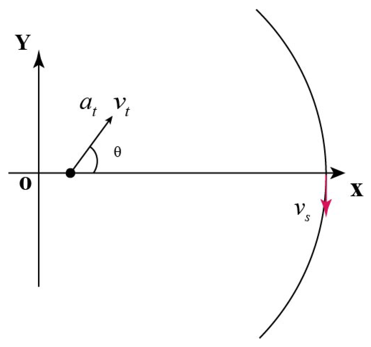
The first example is the basic constant speed target. When considering the symmetrical characteristics of a circular trajectory, there always exists a time at which a constant speed target intercepts the line segment between the radar and the scene center (or crosses the scene center). Thus, we set this moment as the time $t=0$ to build the ground coordinate system. Figure 6 illustrates the target motion at $t=0$. $v_t$, $\theta$, and $x_0$ are the target speed, target heading, and intercept, respectively. Because $H_0$ is not involved in the deduction, the variable is omitted in the following examples.

The target motion functions are shown below

$$\begin{array}{c}\hfill \left\{\begin{array}{cc}\hfill x\left(t\right)& =x_0+v_t·t·cos\theta \hfill \\ \hfill y\left(t\right)& =v_t·t·sin\theta \hfill \\ \hfill v_x\left(t\right)& =v_{t}cos\theta \hfill \\ \hfill v_y\left(t\right)& =v_{t}sin\theta \hfill \end{array}\right.\end{array}$$

(6)

Substitute all target parameters into (1) to obtain the corresponding formulas in the instantaneous radar coordinate system. With proper mathematical operations, the output formulas can be written as (7):

$$\begin{array}{c}\hfill \left\{\begin{array}{cc}\hfill {\tilde{x}}_0\left(t\right)& =R_0-x_{0}cos\left({\omega }_{s}t\right)-v_t·t·cos({\omega }_{s}t-\theta )\hfill \\ \hfill {\tilde{y}}_0\left(t\right)& =x_{0}sin\left({\omega }_{s}t\right)+v_t·t·sin({\omega }_{s}t-\theta )\hfill \\ \hfill {\tilde{v}}_{tx}\left(t\right)& =-v_{t}cos({\omega }_{s}t-\theta )\hfill \\ \hfill {\tilde{v}}_{ty}\left(t\right)& =v_{t}sin({\omega }_{s}t-\theta )\hfill \end{array}\right.\end{array}$$

(7)

When we substitute (7) into the displacement factor k in (3), we can obtain (8) as follows:

$$k\left(t\right)=\frac{v_t}{v_s}[v_{t}t+x_{0}cos\theta -R_{0}cos({\omega }_{s}t-\theta )]$$

(8)

The moving target displacement along the $\tilde{y}$ axis relates to the following three aspects: the target-to-radar-speed ratio (outside brackets), the target motion part (first two terms in brackets), and the radar motion part (last term in brackets).

In the target part, only the target speed $v_t$ and the crossing point $x_0$ influence the shift value. The first term can be interpreted as the travel distance. The second term is the value of the target crossing point projected onto the $O\tilde{O}$ vector.

The last part is the radar motion part, which can be interpreted as the radar trajectory being shifted with a constant phase $\theta$ caused by the target’s heading. The last term reflects the fact that the target delocalization effect in CSAR is influenced by radar heading changes caused by its circular trajectory.

Then, the target displaced location $({\tilde{x}}_1\left(t\right),{\tilde{y}}_1\left(t\right))$ in the instantaneous radar coordinate system can be written as (9).

$$\begin{array}{c}\hfill \left\{\begin{array}{cc}\hfill {\tilde{x}}_1\left(t\right)=& \sqrt{\left[v_t^2{cos}^2({\omega }_{s}t-\theta )\right]·t^2+[2v_t{x}_{0}cos\left({\omega }_{s}t\right)cos\left({\omega }_{s}t\right)-2R_0{x}_{0}cos\left({\omega }_{s}t\right)+}\hfill \\ & \overline{2k\left(t\right)v_{t}sin({\omega }_{s}t-\theta )]·t+[R_0^2+x_0^2{cos}^2\left({\omega }_{s}t\right)-2R_0{x}_{0}cos\left({\omega }_{s}t\right)}\hfill \\ & \overline{+2x_{0}k\left(t\right)sin\left({\omega }_{s}t\right)]-k^2\left(t\right)}\hfill \\ \hfill {\tilde{y}}_1\left(t\right)=& x_{0}sin\left({\omega }_{s}t\right)+v_t·t·sin({\omega }_{s}t-\theta )-k\left(t\right)\hfill \end{array}\right.\end{array}$$

(9)

Considering the complexity of (9), the final formulas of the target image trace in the $XOY$ system remain as an inverse coordinate transform. Thus, the parametric functions of the constant speed moving target are given as

$$\begin{array}{c}\hfill \left\{\begin{array}{cc}\hfill x_2\left(t\right)& =[R_0-{\tilde{x}}_1\left(t\right)]cos\left({\omega }_{s}t\right)+{\tilde{y}}_1\left(t\right)sin\left({\omega }_{s}t\right)\hfill \\ \hfill y_2\left(t\right)& =[R_0-{\tilde{x}}_1\left(t\right)]sin\left({\omega }_{s}t\right)-{\tilde{y}}_1\left(t\right)cos\left({\omega }_{s}t\right)\hfill \end{array}\right.\end{array}$$

(10)

Then, the detailed cases are presented to perform qualitative analysis. The simulation results are also presented to validate the proposed method.

4.1.1. Case 1

In the first case, the target speed was set as 4 m/s. The target moves from the negative half of the x axis to the positive half. The corresponding intercept is zero. Then, we used the target parameters and SAR parameters in Table 1 to generate the corresponding target signal. The SAR image of the moving target is shown in Figure 7. The dashed line is the target’s real trace.

Clearly, the image trace generated by this simple constant speed target can present a complex shape. The shape was not elliptical or hyperbolic, as has been present in conventional linear SAR [14]. In this example, there are three interesting structures, A, B, and C, that should be noted and are labeled with a white arrow. Structures A and C coincide with the target’s real trace, and structure B has the largest shift. Since their main feature relates to the y axis direction, the corresponding $y_2\left(t\right)$ versus azimuth viewing angle $\alpha$ is plotted in Figure 8.

A and C are the tangent position whereby the target’s image trace and its real trace coincide. From Figure 8, these positions are obtained during the time interval where the target velocity is parallel to the radar velocity (i.e., $\alpha =\pm {90}^{\circ }$ or $t_0=\pm 23.5$ s). To demonstrate this, the corresponding formula $y_2\left(t\right)$ at $t_0=\pm 23.5$ s is calculated as (11).

$$y_2\left(t_0\right)=R_0-\sqrt{R_0^2-\frac{v_t^4}{v_s^2}{t}_0^2\pm 2\frac{v_t^3}{v_s}{t}_0^2}$$

(11)

The ± in the last term is because of the $sin$ term generated with the azimuth angle $\pm {90}^{\circ }$. From the above formula, we can see that $y_2\left(t_0\right)$ is controlled by $t_0$ and the ratio $\frac{v_t^2}{v_s}$. By replacing the parameters in case 1, $y_2\left(t_0\right)$ was $0.0589$ and $-0.0589$. The nonzero results mean that the target did not lie on the line crossing radar and scene center. Thus, a squint angle existed. However, considering the size of a resolution cell, the results can be approximated as zero. For the case that the target’s velocity and radar’s heading are parallel, the target signature only has a defocusing effect. Thus, $y_2$ is zero under such a case.

The tip structure B corresponds to the time at which the target velocity is perpendicular to the radar velocity. Thus, it has a maximum shift at this time. From (10), the shift position when $t=0$ is given as (12). Because of the iso-range characteristic, the exact $x_2\left(0\right)$ does not lie on the y axis. $x_2\left(0\right)$ is influenced by the ratio of the target speed and radar speed. Because the radar speed is usually larger than the target speed, and imaging grid spacing may be wide, $x_2\left(0\right)$ can be considered as located along the y axis. The exact shift position value in this case was $(-60,0.0002)$, which matches the analysis.

$$\begin{array}{c}\hfill \left\{\begin{array}{cc}\hfill x_2\left(0\right)& =R_0·(1-\sqrt{1-\frac{v_0^2}{v_s^2}})\hfill \\ \hfill y_2\left(0\right)& =-\frac{v_0{R}_0}{v_s}\hfill \end{array}\right.\end{array}$$

(12)

By replacing the corresponding parameters in (10), we drew the estimated image trace with ‘+’ symbols in Figure 9. From what can be seen in the figure, a perfect agreement between the target signature and the estimated image trace was observed.

4.1.2. Case 2

In this case, the target speed was also 4 m/s. The target moved along the y axis from bottom to top. The corresponding SAR image of this moving target is shown in Figure 10. The target’s real trace is plotted with a dashed line.

From what can be seen in the figure, the target signature was rightward bowing. The tangent position is clearly shown in the image, which is labeled as B. A and C were the tip structures and were not as evident as in case 1. This is because of the differences in the target radar relative motions. In case 1, the target radar relative motion was ‘parallel-perpendicular-parallel’. Therefore, the target signature had two evident tangent positions and an evident tip structure. Compared with case 1, the target radar relative motion was ‘perpendicular-parallel-perpendicular’. Thus, we obtained two partial tip structures and a tangent position in the middle. If the aperture in the simulation was extended to a larger aperture or even ${360}^{\circ }$, the full tip structures could be seen. Therefore, we could obtain the same conclusion that this target image trace is not elliptical or hyperbolic, even if the shape looks similar. Again, perfect agreement was obtained between the estimated image trace and the target signature in Figure 11.

4.1.3. Case 3

In the above cases, we can see interesting structures such as the tangent position and tip structure. Theoretically, two tangent positions as in case 1 can be used for indicating the target’ real trace. Thus, the speed can be roughly calculated by the distance and time between two tangent positions. To further determine the real target moving direction, the tip structure can be used, as shown in this case.

This case simulated two moving targets having the same real trace with opposite moving directions. The target speed was 4 m/s as before, and the intercept remained at zero. The difference here is that the parameter $\theta$ was changed to ${45}^{\circ }$. After BP processing to obtain the target image, we plotted the real trace and the estimated image trace in the same figure, as shown in Figure 12. Target ‘a’ moved from top right to bottom left, and target ‘b’ moved in the opposite direction as target ‘a’. Their signatures are labeled with white arrows. We plotted their estimated image traces with ‘o’ and ‘+’ symbols.The estimated image traces for the two targets matched the SAR image.

From what can be seen in Figure 12, we can see that the target signatures lay on different sides of the real trace. Their tangent positions coincided with the real trace, but the tip pointing directions were different. The tip pointing direction can be interpreted as follows. For target a, it moved away from the radar when their velocity vectors were perpendicular. Thus, the Doppler shift angle was negative, which means that it would shift to the backward position relative to the radar position at that moment. For target b, a similar analysis can be made. Therefore, the tip pointing direction can be used for differentiating the real moving direction.

4.2. Constant Acceleration Target (Type B)

The next type is the constant acceleration target. The geometry is similar to the constant speed target. The top view of the target motion at $t=0$ is shown in Figure 13. Compared with the constant speed target, only one parameter, the acceleration $\overrightarrow{a_t}$, is added. For generality, a typical constant acceleration target is modeled such that $\overrightarrow{a_t}$ and $\overrightarrow{v_t}$ do not coincide. However, the typical model can be regarded as a combination of several simple cases (i.e., $\overrightarrow{a_t}$ and $\overrightarrow{v_t}$ coincide). Thus, in this part, targets with an acceleration $\overrightarrow{a_t}$ and speed $\overrightarrow{v_t}$ along the same direction were analyzed.

The target motion functions are given as follows.

$$\begin{array}{c}\hfill \left\{\begin{array}{cc}\hfill x\left(t\right)& =x_0+v_t·t·cos\theta +\frac{1}{2}{a}_t·t^2·cos\theta \hfill \\ \hfill y\left(t\right)& =v_t·t·sin\theta +\frac{1}{2}{a}_t·t^2·sin\theta \hfill \\ \hfill v_x\left(t\right)& =v_{t}cos\theta +a_t·t·cos\theta \hfill \\ \hfill v_y\left(t\right)& =v_{t}sin\theta +a_t·t·sin\theta \hfill \end{array}\right.\end{array}$$

(13)

In (13), $x_0$ and $v_t$ are the intercept and target speed when $t=0$. $\theta$ is the target heading relative to the positive x axis. $a_t$ is the target acceleration.

Substitute (13) into (1) to obtain the formulas shown below.

$$\begin{array}{c}\hfill \left\{\begin{array}{cc}\hfill {\tilde{x}}_0\left(t\right)=& R_0-x_{0}cos\left({\omega }_{s}t\right)-v_t·t·cos({\omega }_{s}t-\theta )\hfill \\ & -\frac{1}{2}{a}_t·t^2·cos({\omega }_{s}t-\theta )\hfill \\ \hfill {\tilde{y}}_0\left(t\right)=& x_{0}sin\left({\omega }_{s}t\right)+v_t·t·sin({\omega }_{s}t-\theta )\hfill \\ & +\frac{1}{2}{a}_t·t^2·sin({\omega }_{s}t-\theta )\hfill \\ \hfill {\tilde{v}}_{tx}\left(t\right)=& -v_{t}cos({\omega }_{s}t-\theta )-a_t·t·cos({\omega }_{s}t-\theta )\hfill \\ \hfill {\tilde{v}}_{ty}\left(t\right)=& v_{t}sin({\omega }_{s}t-\theta )+a_t·t·sin({\omega }_{s}t-\theta )\hfill \end{array}\right.\end{array}$$

(14)

Then, we use (14) and (3) to calculate the displacement factor $k\left(t\right)$ and obtain (15).

$$\begin{array}{cc}\hfill k\left(t\right)=& \frac{v_t}{v_s}\{x_{0}cos\theta +[v_t+\frac{x_0{a}_t}{v_t}cos\theta -\frac{R_0{a}_t}{v_t}cos({\omega }_{s}t-\theta )]t\hfill \\ \hfill & +\frac{3}{2}{a}_t{t}^2+\frac{1}{2v_t}{a}_t^2{t}^3-R_{0}cos({\omega }_{s}t-\theta )\}\hfill \end{array}$$

(15)

Equation (15) is arranged in similar form as the displacement factor for the constant speed target. The value outside the bracket is the ratio of the target speed (at $t=0$) and the radar speed.Inside the bracket, the first four terms from zeroth order to third order are the target motion part. When compared to (8), the acceleration parameter influences the first order term. In addition, we added the second and third order terms. The zeroth order term and the last term in the radar motion part have the same form as (8).

Then, the target image position in the instantaneous radar coordinate system is given as (16). The form ${\tilde{y}}_2$ is simple when compared to the formula for ${\tilde{x}}_2$. Compared to ${\tilde{y}}_2$ in (9), only a second-order term is added. The added second-order term represents the target acceleration’s influence on the target image position in the instantaneous radar coordinate system. The ${\tilde{x}}_2$ has a more complex form. All terms are arranged as power series.

$$\begin{array}{c}\hfill \left\{\begin{array}{cc}\hfill {\tilde{x}}_1\left(t\right)=& \sqrt{[R_0^2-2R_0{x}_{0}cos\left({\omega }_{s}t\right)+x_0^2{cos}^2\left({\omega }_{s}t\right)+2x_{0}sin\left({\omega }_{s}t\right)k\left(t\right)]+[2x_0{v}_{t}cos({\omega }_{s}t-\theta )}\hfill \\ & \overline{+2v_{t}sin({\omega }_{s}t-\theta )k\left(t\right)-2R_0{v}_{t}cos({\omega }_{s}t-\theta )]t+[x_0{a}_{t}cos\left({\omega }_{s}t\right)cos({\omega }_{s}t-\theta )}\hfill \\ & \overline{+v_t^2{cos}^2({\omega }_{s}t-\theta )-R_0{a}_{t}cos({\omega }_{s}t-\theta )+\frac{1}{2}{a}_{t}k\left(t\right)sin(2{\omega }_{s}t-2\theta )]t^2}\hfill \\ & \overline{+a_t{v}_t·t^3·{cos}^2({\omega }_{s}t-\theta )+\frac{1}{4}{a}_t^2·t^4·{cos}^2({\omega }_{s}t-\theta )-k^2\left(t\right)}\hfill \\ \hfill {\tilde{y}}_1\left(t\right)=& x_{0}sin\left({\omega }_{s}t\right)+v_t·t·sin({\omega }_s-\theta )t+\frac{1}{2}{a}_t·t^2·sin({\omega }_{s}t-\theta )-k\left(t\right)\hfill \end{array}\right.\end{array}$$

(16)

We applied the inverse transformation to (16). For the same consideration, the output target image trace in the ground coordinate system is written as (17).

$$\begin{array}{c}\hfill \left\{\begin{array}{cc}\hfill x_2\left(t\right)& =[R_0-{\tilde{x}}_1\left(t\right)]cos\left({\omega }_{s}t\right)+{\tilde{y}}_1\left(t\right)sin\left({\omega }_{s}t\right)\hfill \\ \hfill y_2\left(t\right)& =[R_0-{\tilde{x}}_1\left(t\right)]sin\left({\omega }_{s}t\right)-{\tilde{y}}_1\left(t\right)cos\left({\omega }_{s}t\right)\hfill \end{array}\right.\end{array}$$

(17)

Next, the simulation experiments are given to demonstrate the effectiveness of predicting the constant acceleration target’s image trace using the above formulas.

Compared with the constant speed target, only one parameter is added. Two cases (acceleration and deceleration) were simulated to show the influence of the acceleration parameter. The two cases have similar simulation configurations. The SAR parameters in Table 1 were used as before. The moving targets moved from the positive x axis to the negative part, and the intercept is zero. The target speed (at $t=0$) was −4 m/s. For the acceleration and deceleration cases, the value of $a_t$ was −0.1 m/s² and 0.1 m/s², respectively.

Then, we applied the BP algorithm to obtain the images of the moving targets, as shown in Figure 14. Figure 14a,b show the signatures of the deceleration target and acceleration target, respectively. Their real traces are plotted with dashed lines.

In this example, the tangent position and the tip structures also appeared. The tip structure also lay on the y axis. From what was derived in (17), the shift position is given as below.

$$\begin{array}{c}\hfill \left\{\begin{array}{cc}\hfill x_2\left(0\right)& =R_0·(1-\sqrt{1-\frac{v_t^2}{v_s^2}})\hfill \\ \hfill y_2\left(0\right)& =-\frac{v_t{R}_0}{v_s}\hfill \end{array}\right.\end{array}$$

(18)

It is not surprising to see that (18) has the same form as (12), since the shift value is dominated by the instantaneous speed as in (3). Therefore, we can see that the original $v_0$ is replaced by the initial speed $v_t$.

The difference here is that the tip pointing direction has changed. In the previous subsection, for case 1, the target signature showed a symmetry, as in Figure 7. The tip pointing direction was almost perpendicular to the x axis. Because of the constant speed, the travel distances before and after the origin were equal. Therefore, its image trace had a symmetrical shape. Here, as in Figure 14a, the deceleration made the travel distance before the origin longer than the part after passing the origin. This caused the unequal length of the image trace on both sides of the tip structure. It changed the tip pointing direction. Similar analysis can be conducted for the acceleration case.

We plotted the estimated image trace on two images, as shown in Figure 15. Here, the estimated image trace matched the target signature, which validated the proposed method of type B.

4.3. Constant Rotating Speed Target (Type C)

In the previous sections, the proposed method was validated with basic linearly moving targets. This section analyzes rotating target’s signature to show the effectiveness for nolinear moving targets.

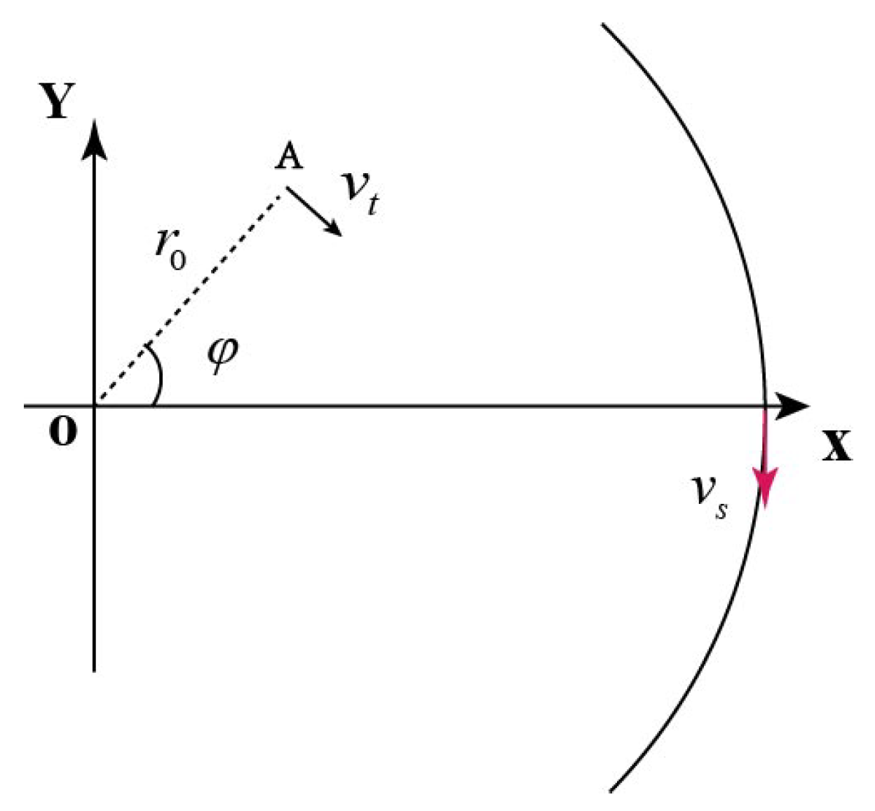
Figure 16 is the top view of the target motion at $t=0$. The target locates at position A at $t=0$. $v_t$ is the rotating speed, $r_0$ is the rotating radius, and $\phi$ is the angle (at $t=0$) between the $OA$ and x axes. The target motion functions are given by (19).

$$\begin{array}{c}\hfill \left\{\begin{array}{cc}\hfill x\left(t\right)& =r_{0}cos({\omega }_{s}t+\phi )\hfill \\ \hfill y\left(t\right)& =r_{0}sin({\omega }_{s}t+\phi )\hfill \\ \hfill v_x\left(t\right)& =v_{t}sin({\omega }_{s}t+\phi )\hfill \\ \hfill v_y\left(t\right)& =-v_{t}cos({\omega }_{s}t+\phi )\hfill \end{array}\right.\end{array}$$

(19)

We applied transformation (1) to (19). The obtained transformed functions are as follows.

$$\begin{array}{c}\hfill \left\{\begin{array}{cc}\hfill {\tilde{x}}_0\left(t\right)=& R_0-r_{0}cos[({\omega }_s-{\omega }_t)t-\phi ]\hfill \\ \hfill {\tilde{y}}_0\left(t\right)=& r_{0}sin[({\omega }_s-{\omega }_t)t-\phi ]\hfill \\ \hfill {\tilde{v}}_{tx}\left(t\right)=& v_{t}cos[({\omega }_s-{\omega }_t)t-\phi ]\hfill \\ \hfill {\tilde{v}}_{ty}\left(t\right)=& v_{t}sin[({\omega }_s-{\omega }_t)t-\phi ]\hfill \\ \hfill {\omega }_t=& \frac{v_t}{r_0}\hfill \end{array}\right.\end{array}$$

(20)

For deduction convenience, $v_t/r_0$ was rewritten as the target angular speed ${\omega }_t$. The output formulas present a simple form. This is because the target model is composed of trigonometric functions. The complexity can be reduced by proper deduction. For the same reason, the form of the target image trace functions in the instantaneous radar coordinate system is also simple. The corresponding results are given as follows.

$$\begin{array}{c}\hfill \left\{\begin{array}{cc}\hfill {\tilde{x}}_1\left(t\right)=& \sqrt{R_0^2+r_0^2-2R_0{r}_{0}cos[({\omega }_s-{\omega }_t)t-\phi ]}\hfill \\ & \overline{-{(\frac{{\omega }_s-{\omega }_t}{{\omega }_s})}^2{r}_0^{2}sin[({\omega }_s-{\omega }_t)t-\phi ]}\hfill \\ \hfill {\tilde{y}}_1\left(t\right)=& \frac{{\omega }_s-{\omega }_t}{{\omega }_s}{r}_{0}sin[({\omega }_s-{\omega }_t)t-\phi ]\hfill \end{array}\right.\end{array}$$

(21)

Then, we applied the inverse transformation to obtain target image trace functions in the ground coordinate system. The final form is shown in the previous section, i.e., (22).

$$\begin{array}{c}\hfill \left\{\begin{array}{cc}\hfill x_2\left(t\right)& =[R_0-{\tilde{x}}_1\left(t\right)]cos\left({\omega }_{s}t\right)+{\tilde{y}}_1\left(t\right)sin\left({\omega }_{s}t\right)\hfill \\ \hfill y_2\left(t\right)& =[R_0-{\tilde{x}}_1\left(t\right)]sin\left({\omega }_{s}t\right)-{\tilde{y}}_1\left(t\right)cos\left({\omega }_{s}t\right)\hfill \end{array}\right.\end{array}$$

(22)

Then, simulation experiments were presented to demonstrate the method.

The influence of the rotating direction was first examined. Two targets were set with different rotating directions: one target moved clockwise, and the other moved counter-clockwise. The remaining parameters were the same. The speed $v_t$, rotating radius $r_0$, and angle $\phi$ were 4 m/s, 100 m, and $0^{\circ }$, respectively. Then, we used the previous radar parameters to generate the signal. We next applied the BP algorithm to obtain their SAR images, as in Figure 17.

Figure 17a,b are SAR images of the target moving in the clockwise and counter-clockwise direction, respectively. The real trace is plotted with a ‘-’ line. The target rotated angle in the simulation was less than ${180}^{\circ }$, because the target’s angular speed was less than the radar’s angular speed.

In Figure 17a, there is only one tangent position, because the radar and target move in the same direction; there was no perpendicular case in this example. The radar and target are parallel when $t=0$. This makes only one tangent position exist. In addition, its image trace lies inside the real trace. This can be explained as follows. When $t<0$, the target moves away from the radar, and it generates a negative Doppler shift angle (relative to the line of sight). When $t>0$, the target moves toward the radar, and a positive Doppler shift angle is generated. Hence, its image trace is bent inside the real trace.

Figure 17b has two tip structures and one tangent position. This is because the relative motion between radar and target is ‘perpendicular-parallel-perpendicular’. Its image trace lies outside the real trace when compared to the target in Figure 17a. This is because the target’s rotating direction was different from the radar’s direction. This generated positive and negative Doppler shift angles before and after $t=0$. Thus, its image trace lay outside the real trace.

When we plotted the estimated image trace of the two targets on their SAR images as in Figure 18, we found that the estimation matched the target signature perfectly.

Next, a target with clockwise motion and non-zero $\phi$ was simulated. The remaining parameters were the same as the target in Figure 17a, while $\phi$ was set to ${20}^{\circ }$. The SAR image is shown in Figure 19. The real trace and the estimated image trace are plotted in the same figure. Compared tp Figure 17a, the tangent position moved to the upper area. Because $\phi \ne 0$, the time at which the target and radar became parallel shifted to the negative part of azimuth time. Thus, $\phi$ can influence the tangent position’s location. Furthermore, the estimated image trace was in perfect agreement with the target signature. Thus, the method’s effectiveness on nonlinearly moving targets is demonstrated.

5. Real Data Experiment

In this section, we used single-channel data of the X band GOTCHA dataset to conduct an analysis of the moving target image trace estimation with the proposed method. The proposed method is more flexible, because it only requires the instantaneous speeds and positions of radar and target. Comparing to simulated data wherein all parameters and error factors can be controlled, the real data unavoidably contain some error sources such as recorded deviated SAR’s and moving target’s trajectory due to accuracy limitation of the GPS instrument, as well as unknown 3D terrain information of the scenario that the target moved onto. In simulated data, these factors can be well controlled as zero; hence, the processed result will match the target signature perfectly as in previous sections, while, in real data, these factors would cause minor mismatches in the output result. Because the open dataset does not provide all of the error factors’ data, we extracted mismatches in processed result to conduct partial quantitative analysis. In this way, we evaluated the method’s estimation performance on real data.

To calculate the target’s image trace in the CSAR image, information about the target and platform is needed. The position along the $x,y,z$ axis and the speed of the target car is shown in Figure 20. The sample rate of the target GPS was 1 Hz lower than the radar’s PRF of 2171.6 Hz. Therefore, the target’s position and speed should be interpolated at the radar’s sampling time. Here, the cubic interpolation method was adopted to obtain a smooth curve. The proposed method only used the position and velocity (the vertical speed and position were also added to achieve the estimation) at each sample time. Thus, we could still compute the target’s image trace, even in a real scenario. Since the DEM of this area was not provided, the target’s image trace in the ground plane was calculated as shown in Figure 21.

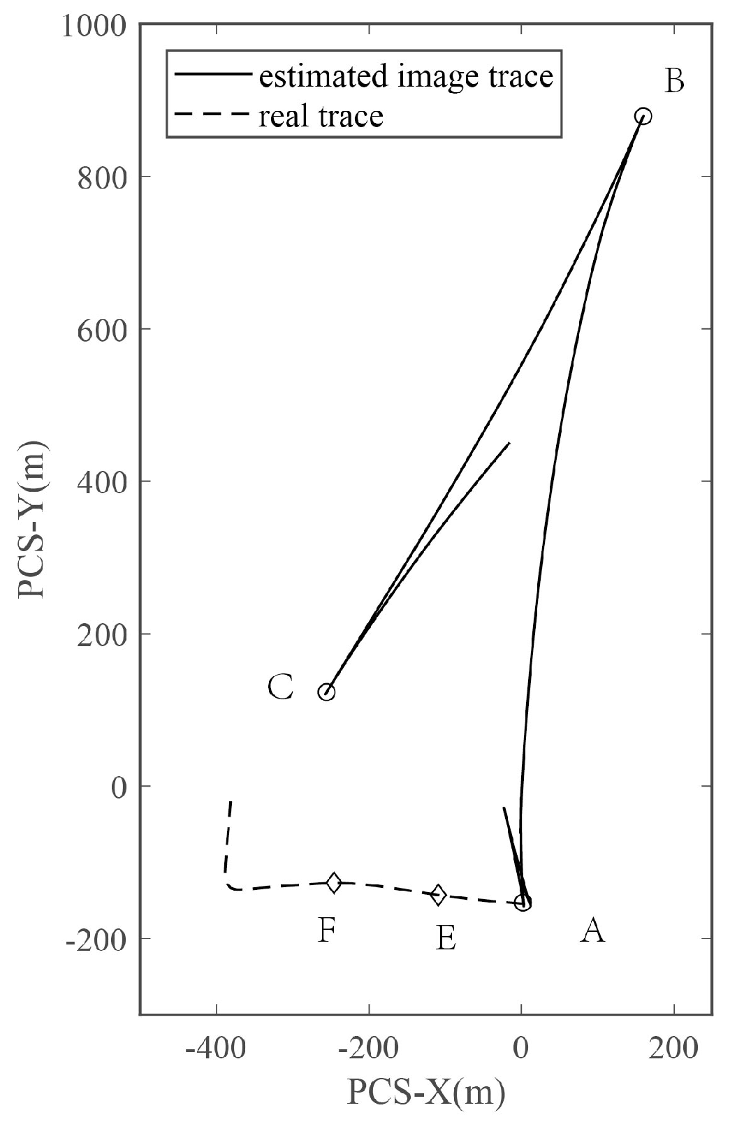
Figure 21 shows the result calculated with all 71 s of data; the dashed line represents the real trace in the ground plane, and the solid line represents the calculated image trace. The image trace can be analyzed according to the part separated by points A, B, and C labeled with a circle. Points A, B, and C correspond to times of 23.2 s, 44.6 s, and 63.2 s, respectively. Point A shows where the target passed the intersection and started to accelerate along the road. The target motion before 23.2 s generated a small segment image trace near point A. As shown in Figure 20d for 0–23.2 s, the car moved and stopped during this interval. Thus, the target signature shifted and subsequently returned to its real position. The segment ABC was generated by the target’s motion along the road, which can be regarded as linear motion. The car was accelerating during 23.2–44.6 s and decelerating from 44.6 to 63.2 s. The tip structure B generated in this interval points to the right slightly, showing similar characteristics as the accelerating case for type B. Thus, we verify the previous analysis. After 63.2 s, the target turned toward the direction along the positive axis of PCS-Y.

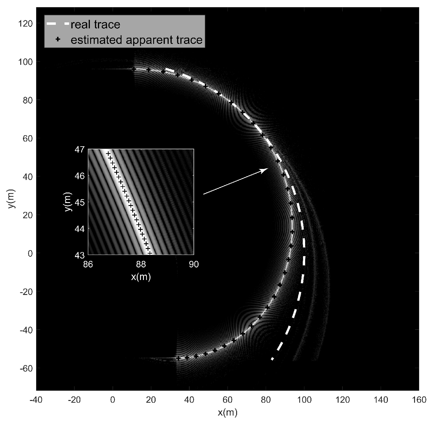
To further demonstrate the accuracy between the estimated image trace and the target signature in SAR imagery, two small scene have been selected. Figure 22a is the SAR image of the selected small scene 1, similar to Figure 1. The azimuth time interval was 37.1–47.2 s, and the corresponding target’s real trace was from point E to point F in Figure 21. The SAR image spacing was 1 m. The target ‘v’-shaped signature lay at the center of the image. Compared to its signature, the estimated image trace lay on the region close to the signature in Figure 22a. By comparing Figure 22a,b, we see two differences. The first difference is that the estimated image trace does not exactly match the target signature. The tip position was (147,919) m in Figure 22a and (159,878) m in Figure 22b. The estimated image trace had offsets about 41 m along the Y axis and 12 m along the X axis compared with the target signature. These results consider the GPS’s low sample rate, fast change of the target’s z position (−0.46 m to −9.53 m) at this interval, and the recorded GPS height error of 7 m in the dataset (although this error is processed as denoted in the dataset) [21]. A reasonable cause is the residual GPS height error. The error in the target position along the z axis made the estimated image trace lie in the wrong range. In addition, because the target speed along the z direction is calculated via the target’s z position, there was a deviation in the Doppler shift. Therefore, the offsets along both the X axis and Y axis in Figure 22 were generated.

The second difference is that the lengths of both sides of the ‘v’-shaped structure were not equal in (b), whereas they were almost equal in Figure 22a. An explanation for this is that there might still exist a GPS time offset even if it is preprocessed, as mentioned in [21]. The GPS time offset provided in dataset was (0.9 s).

The small scene 2 is shown in Figure 23. The corresponding azimuth time interval was 25.7–26.7 s, when target was passing the intersection. Here, we can still see the difference mentioned above. One is the position offset, the other one is the length. The offsets (using position of the upper end) in this case were about 4 m along x direction and 52 m along y direction. Because the target height almost did not change (the height is 0.7 m) at this interval, the offset was smaller than in scene 1.

Considering the errors in the above example, this method achieved a good estimation ability on real data. If accurate target position and velocity data can be obtained, the proposed method can predict the corresponding image trace.

6. Discussion

The purpose of this part is to show the differences in image traces between CSAR and linear SAR and to demonstrate the necessity of the proposed method for predicting target’s image trace in CSAR. To the best of our knowledge, the previous linear SAR image trace function deduction method [16] has been discussed based on point target simulation, and the paper applying it to real data has not been published. Hence, the comparison of the proposed method and [16] on point target simulation (using target type A) is given.

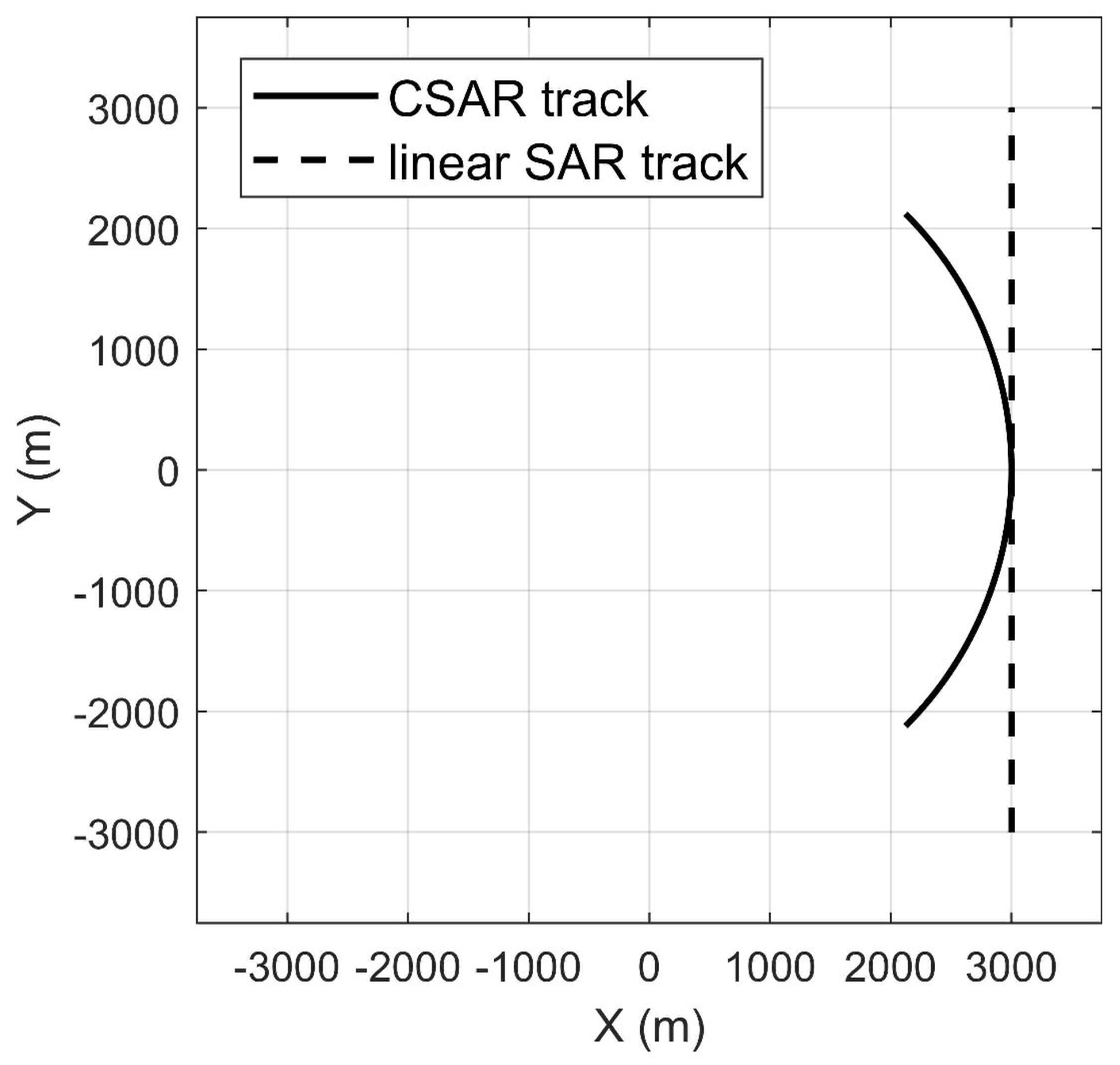
Most radar system parameters for the simulation are the same in Table 1. For two examples, the radar works in side-looking mode. Since the linear SAR can not illuminate the scene for ${180}^{\circ }$ in practice, the azimuth integration angle ${\theta }_{azi}$ was 90° (45°~−45°) for both cases. For linear SAR, another difference is that the $R_0$ becomes a minimum ground range to the scene center. The top view of the geometry is shown in Figure 24. Thus, the x axis becomes the range direction, and the y axis becomes the azimuth direction for the linear SAR case.

For a constant speed target in linear SAR, the moving target effects (smearing/ delocalization) are simply driven by range speed and azimuth speed [1]. Two ideal constant speed point targets are set for the simulation; their speeds are both 2 m/s. One moves along the y axis (azimuth direction) from bottom to the top (example 1); another one moves along the x axis (range direction) from right to the left (example 2). For convenience, the targets lie on origin when $t=0$.

The proposed method is demonstrated for the CSAR case in previous sections. The compared method is proposed by David Garren [16], which is based on the linear SAR case. The deduced results of the constant speed target in [16] are presented with notations in our paper.

$$\begin{array}{c}\hfill \left\{\begin{array}{cc}\hfill x\left(t\right)& =x_0-\frac{v_{t}sin\theta }{{\kappa }_0}{t}^2\hfill \\ \hfill y\left(t\right)& =y_0+{\kappa }_0·v_{t}cos\theta +2v_{t}sin\theta ·t\hfill \\ \hfill {\kappa }_0& =-\frac{R_0}{v_s}\hfill \end{array}\right.\end{array}$$

(23)

where ${\kappa }_0$ is the temporal constant. Because the platform moves from top to the bottom, it is a negative value according to [16]. $(x_0,y_0)$ is the target position at $t=0$. $v_t$ and $\theta$ are target speed and heading, respectively. In (23), the parametric functions form a parabola curve stretched along y axis. The $y\left(t\right)$ is linear form with three terms. The first two terms are the target shifted center location in the linear SAR image. The offset value ${\kappa }_0·v_{t}cos\theta$ is controlled by range speed. The third term shows that the smearing effect is governed by the azimuth speed. Compared to (10), the shape of the image trace in the linear SAR does not depend on azimuth viewing. Once the target’s speed and heading are set, the image trace is fixed, while in (10), the target image trace shape in CSAR is influenced by the azimuth viewing angle. This is the main reason for the shape differences in two modes as will be presented. Next, we used (10) and (23) to predict the two target’s image traces.

6.1. Example 1

First is the target with azimuth speed(moves along the y axis). Its image traces under CSAR and linear SAR conditions are shown in Figure 25. The ‘$-o-$’ and ‘$-+-$’ line denote the CSAR(our method) and linear SAR(Garren’s method) results, respectively. From what can be seen in Figure 25, the image traces in the linear SAR are longer than in CSAR. It means that the smearing effect is more severe in the linear SAR. This is because the azimuth direction is not fixed in CSAR. The instantaneous azimuth direction is varying in CSAR. For different viewing angles, the target’s azimuth speed component is a projection of its real speed. In this case, the target instantaneous azimuth speed reached a maximum value of 2 m/s when $t=0$. This component was smaller at other azimuth viewing angle, thereby mitigating the smearing effect.

From what can be seen in Figure 25, we can also notice that part of the image traces are coincided. This means that, in limited aperture, the image trace in CSAR can be predicted with the linear SAR model. Since the proposed method was demonstrated to be effective, we evaluated the approximation performance along x and y directions with the following formulas.

$$\begin{array}{c}\hfill \left\{\begin{array}{c}\hfill x_{lin}\left({\theta }_{azi}\right)-x_{cir}\left({\theta }_{azi}\right)>{\delta }_x\\ \hfill y_{lin}\left({\theta }_{azi}\right)-y_{cir}\left({\theta }_{azi}\right)>{\delta }_y\end{array}\right.\end{array}$$

(24)

where $x_{lin}\left({\theta }_{azi}\right)$ and $y_{lin}\left({\theta }_{azi}\right)$ are the parametric functions in (23). To characterize this limited aperture, the azimuth time t is replaced with azimuth viewing angle ${\theta }_{azi}$. $x_{cir}\left({\theta }_{azi}\right)$ and $y_{cir}\left({\theta }_{azi}\right)$ are (10) with similar notation. The ${\delta }_x$ and ${\delta }_y$ are the dimension of the resolution cell. They can be calculated via CSAR resolution formulas given in [29]. Using the simulation parameters, the corresponding resolutions were ${\delta }_x$ = 0.12 m and ${\delta }_y$ = 0.03 m. Then, the x,y components of the image traces predicted by two models versus azimuth viewing angle ${\theta }_{azi}$ are plotted in Figure 26. The results of CSAR and linear SAR are plotted with dashed line and solid line, respectively. The circle on the curves denotes the limit aperture calculated via (24). In Figure 26a, the aperture value was $44.8^{\circ }(-22.4^{\circ },22.4^{\circ })$ along the x axis. The aperture value along the y axis was $18.6^{\circ }(-9.3^{\circ },9.3^{\circ })$. Thus, for the this azimuth speed target, the limit aperture for the linear SAR model was $18.6^{\circ }$. In practice, all ${90}^{\circ }$ cannot be integrated due to the target’s anisotropic scattering behavior. The resolution ${\delta }_x,{\delta }_y$ will be smaller. Therefore the tolerated aperture value for the linear SAR model could be even larger.

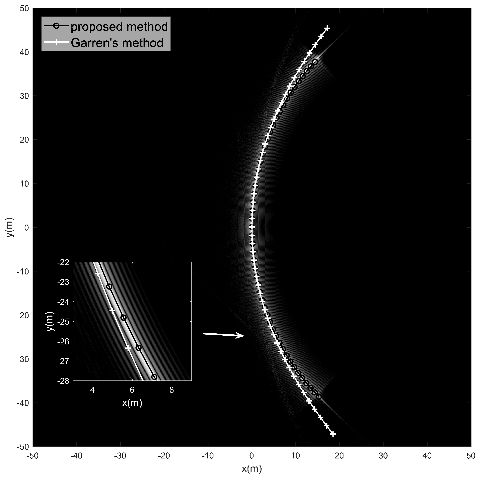
To verify the analysis above, we plotted the estimated image traces on the SAR image generated by the BP algorithm. The result is shown in Figure 27. The notations are the same as in Figure 25. The proposed method matched the target signature, while the result (using Garren’s method) only matched part of it. This can be seen in the enlarged picture clearly. The result predicted by Garren’s method started to deviate from the target signature. Thus, Garren’s method failed to predict the image trace in CSAR. This is because the platform’s velocity vector varies along time, while it is fixed in traditional linear SAR.

6.2. Example 2

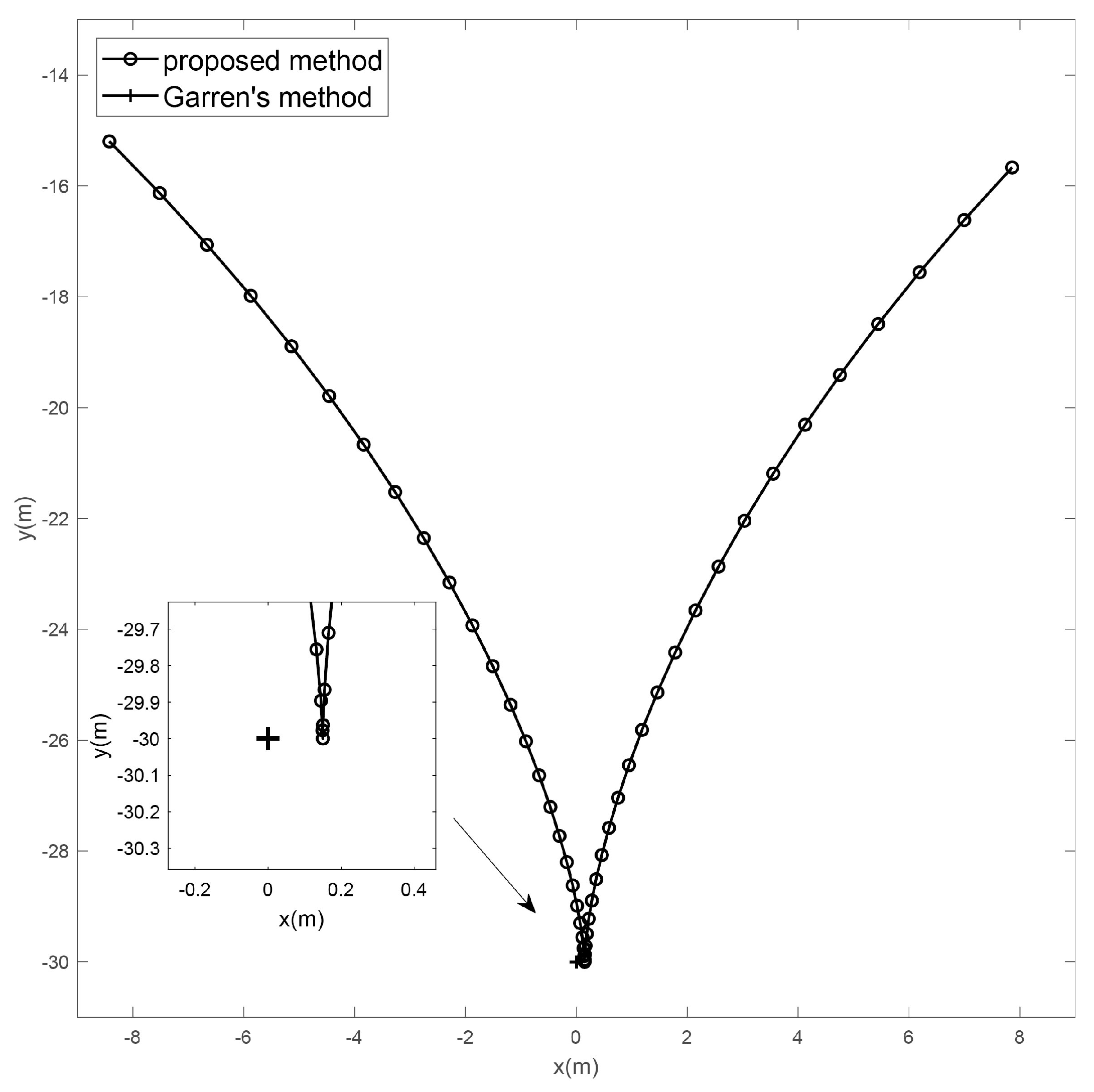
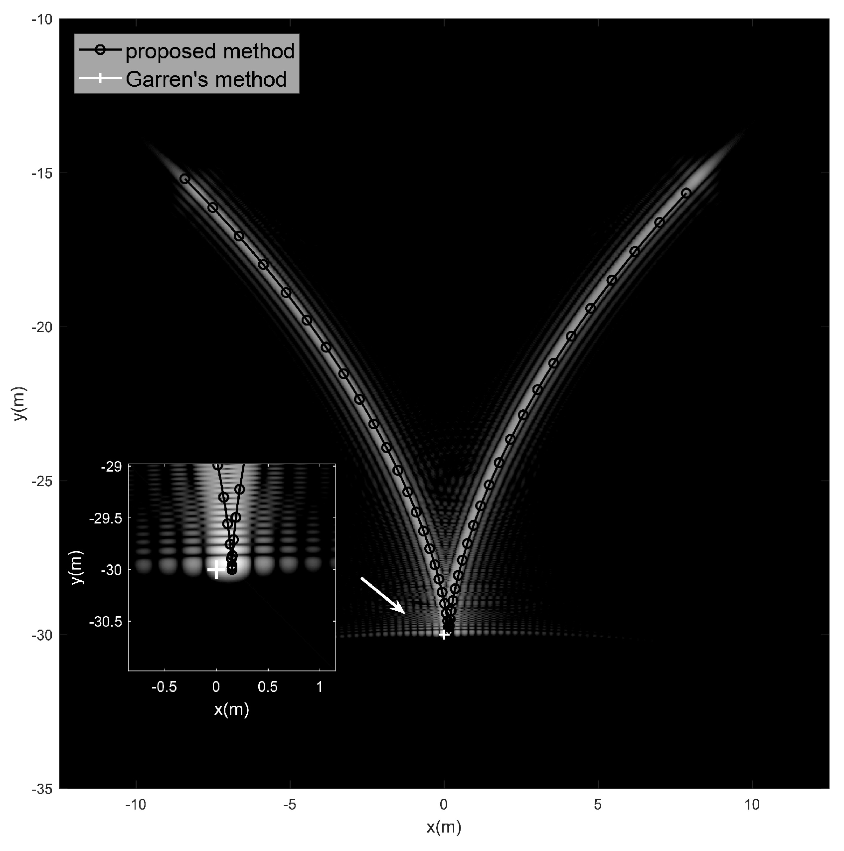
Next is the example of target with range speed. The calculated image traces are shown in Figure 28. In this example, the difference is quiet clear. The CSAR result presents the ‘V’ shaped structure, while the linear SAR result is only a dot, as shown in the enlarged picture. The reasons are the following: (1) azimuth and range direction are fixed in linear SAR; (2) range speed targets present delocalization rather than smearing effect in linear SAR. It would be clear by looking into (23). When the target only has range speed, the (23) become constant as shown below.

$$\begin{array}{c}\hfill \left\{\begin{array}{cc}\hfill x\left(t\right)& =x_0\hfill \\ \hfill y\left(t\right)& =y_0+{\kappa }_0·v_{t}cos\theta \hfill \\ \hfill {\kappa }_0& =-\frac{R_0}{v_s}\hfill \end{array}\right.\end{array}$$

(25)

Thus, the predicted result is a point in the image. For CSAR, the target’s velocity vector was perpendicular to the radar’s velocity vector only at $t=0$. For the rest of the time, the target has both instantaneous range speed and azimuth speed because of circular geometry. Therefore, the generated signature has a complex shape in CSAR.

As before, we plotted the curve of the $x,y$ components of image traces predicted by two models versus the azimuth viewing angle ${\theta }_{azi}$ as shown in Figure 29. The aperture value along the x axis was $11.6^{\circ }(-5.8^{\circ },5.8^{\circ })$, while the value along the y axis was $3.{92}^{\circ }(-1.{96}^{\circ },1.{96}^{\circ })$. Thus, the limit aperture for this range speed target was $3.{92}^{\circ }$ smaller than the value in the previous azimuth speed target example.

Again, the SAR image superimposed with predicted image traces is shown in Figure 30. From the figure results, we can see that the result matches the analysis above. The predicting performance of using Garren’s method decreased severely when applying to this range speed target.

7. Conclusions

In this paper, a new method for deducing the parametric functions of a moving target’s image traces in single-channel CSAR imagery was presented. It was assumed that the radar follows a circular trajectory in side-looking mode and that the target moves on the ground plane.

The proposed method combined the range-Doppler equations and Cartesian transformation between the ground coordinate system and the instantaneous radar coordinate system to deduce the parametric functions. Three types of targets (constant speed, constant acceleration, and rotating around the scene center at constant speed) were analyzed with the proposed method. The point target simulations of those moving targets showed perfect agreement between the estimated image trace and the target’s signature. The proposed method was conducted and analysis performed with both simulated and real data. Moreover, in a real scenario, if accurate radar–target position and velocity data are provided, the proposed method can predict the exact target image trace.

The future work will be to conduct the comparison between existing linear SAR image trace estimation methods in real data scenario to further reveal the difference of the methods. The second one involves using proposed methods to analyze the performance and limitations of the image-sequence-based CSAR GMTI method. The third one will be to develop speed estimation and refocusing methods based on signature analysis for CSAR.

References

- Raney, R.K. Synthetic Aperture Imaging Radar and Moving Targets. IEEE Trans. Aerosp. Electron. Syst. 1971, AES-7, 499–505. [Google Scholar] [CrossRef]
- Ender, J.H.G. Space-time processing for multichannel synthetic aperture radar. Electron. Commun. Eng. J. 1999, 11, 29–38. [Google Scholar] [CrossRef]
- Makhoul, E.; Baumgartner, S.V.; Jager, M.; Broquetas, A. Multichannel SAR-GMTI in Maritime Scenarios With F-SAR and TerraSAR-X Sensors. IEEE J. Sel. Top. Appl. Earth Obs. Remote Sens. 2015, 8, 5052–5067. [Google Scholar] [CrossRef]
- Chapin, E.; Chen, C.W. Airborne along-track interferometry for GMTI. IEEE Aerosp. Electron. Syst. Mag. 2009, 24, 13–18. [Google Scholar] [CrossRef]
- Vu, V.T.; Sjogren, T.K.; Pettersson, M.I.; Gustavsson, A.; Ulander, L.M. Detection of moving targets by focusing in UWB SAR Theory and experimental results. IEEE Trans. Geosci. Remote Sens. 2010, 48, 3799–3815. [Google Scholar] [CrossRef]
- Fienup, J.R. Detecting moving targets in SAR imagery by focusing. IEEE Trans. Aerosp. Electron. Syst. 2001, 37, 794–809. [Google Scholar] [CrossRef]
- Lin, Y.; Hong, W.; Tan, W.; Wang, Y.; Xiang, M. Airborne circular SAR imaging: Results at P-band. In Proceedings of the 2012 IEEE International Geoscience and Remote Sensing Symposium, Munich, Germany, 22–27 July 2012; pp. 5594–5597. [Google Scholar] [CrossRef]
- Frolind, P.O.; Gustavsson, A.; Lundberg, M.; Ulander, L.M.H. Circular-Aperture VHF-Band Synthetic Aperture Radar for Detection of Vehicles in Forest Concealment. IEEE Trans. Geosci. Remote Sens. 2012, 50, 1329–1339. [Google Scholar] [CrossRef]
- Cantalloube, H.M.J.; Koeniguer, E.C.; Oriot, H. High resolution SAR imaging along circular trajectories. In Proceedings of the 2007 IEEE International Geoscience and Remote Sensing Symposium, Barcelona, Spain, 23–27 July 2007; pp. 850–853. [Google Scholar] [CrossRef]
- Hong, W.; Li, Y.; Tan, W.; Wang, Y.; Xiang, M. Study on geosynchronous circular SAR. J. Radars 2015, 4, 241–253. [Google Scholar]
- Zeng, T.; Yin, W.; Ding, Z.; Long, T. Motion and Doppler Characteristics Analysis Based on Circular Motion Model in Geosynchronous SAR. IEEE J. Sel. Top. Appl. Earth Obs. Remote Sens. 2016, 9, 1132–1142. [Google Scholar] [CrossRef]
- Shen, W.; Lin, Y.; Yu, L.; Xue, F.; Hong, W. Single Channel Circular SAR Moving Target Detection Based on Logarithm Background Subtraction Algorithm. Remote Sens. 2018, 10, 742. [Google Scholar] [CrossRef] [Green Version]
- Poisson, J.B.; Oriot, H.M.; Tupin, F. Ground Moving Target Trajectory Reconstruction in Single-Channel Circular SAR. IEEE Trans. Geosci. Remote Sens. 2015, 53, 1976–1984. [Google Scholar] [CrossRef] [Green Version]
- Jao, J.K. Theory of synthetic aperture radar imaging of a moving target. IEEE Trans. Geosci. Remote Sens. 2001, 39, 1984–1992. [Google Scholar] [CrossRef] [Green Version]
- Moyer, L.R.; Govoni, M.A. Moving target trajectories in low-frequency SAR imagery. IEEE Trans. Aerosp. Electron. Syst. 2014, 50, 2354–2360. [Google Scholar] [CrossRef]
- Garren, D.A. Smear signature morphology of surface targets with arbitrary motion in spotlight synthetic aperture radar imagery. IET Radar Sonar Navig. 2014, 8, 435–448. [Google Scholar] [CrossRef]
- Garren, D.A. Theory of Two-Dimensional Signature Morphology for Arbitrarily Moving Surface Targets in Squinted Spotlight Synthetic Aperture Radar. IEEE Trans. Geosci. Remote Sens. 2015, 53, 4997–5008. [Google Scholar] [CrossRef]
- Garren, D.A. Signature Morphology Effects of Squint Angle for Arbitrarily Moving Surface Targets in Spotlight Synthetic Aperture Radar. IEEE Trans. Geosci. Remote Sens. 2015, 53, 6241–6251. [Google Scholar] [CrossRef]
- Chapman, R.D.; Hawes, C.M.; Nord, M.E. Target Motion Ambiguities in Single-Aperture Synthetic Aperture Radar. IEEE Trans. Aerosp. Electron. Syst. 2010, 46, 459–468. [Google Scholar] [CrossRef]
- Gorham, L.A.; Moore, L.G. SAR image formation toolbox for MATLAB. SPIE 2010, 7699, 769906. [Google Scholar] [CrossRef]
- Scarborough, S.M.; Casteel, C.H., Jr.; Gorham, L.; Minardi, M.J.; Majumder, U.K.; Judge, M.G.; Zelnio, E.; Bryant, M.; Nichols, H.; Page, D. A challenge problem for SAR-based GMTI in urban environments. SPIE 2009, 7337, 73370G. [Google Scholar] [CrossRef]
- Deming, R.W. Along-track interferometry for simultaneous SAR and GMTI: Application to Gotcha challenge data. In Algorithms for Synthetic Aperture Radar Imagery XVIII; Zelnio, E.G., Garber, F.D., Eds.; International Society for Optics and Photonics: Bellingham, WA, USA, 2011; Volume 8051, p. 80510P. [Google Scholar] [CrossRef]
- Barber, B. Indication of slowly moving ground targets in non-Gaussian clutter using multi- channel synthetic aperture radar. IET Signal Process. 2012, 6, 424–434. [Google Scholar] [CrossRef]
- Deming, R.; Best, M.; Farrell, S. Simultaneous SAR and GMTI using ATI/DPCA. In Algorithms for Synthetic Aperture Radar Imagery XXI; Zelnio, E., Garber, F.D., Eds.; International Society for Optics and Photonics: Bellingham, WA, USA, 2014; Volume 9093, p. 90930U. [Google Scholar] [CrossRef]
- Riedl, M.; Potter, L.; Bryant, C.; Ertin, E. Joint synthetic aperture radar and space-time adaptive processing on a single receive channel. IEEE Trans. Aerosp. Electron. Syst. 2015, 51, 331–341. [Google Scholar] [CrossRef]
- Greenewald, K.; Zelnio, E.; Hero, A.H. Robust SAR STAP via Kronecker decomposition. IEEE Trans. Aerosp. Electron. Syst. 2016, 52, 2612–2625. [Google Scholar] [CrossRef] [Green Version]
- An, D.; Wang, W.; Zhou, Z. Refocusing of Ground Moving Target in Circular Synthetic Aperture Radar. IEEE Sens. J. 2019, 19, 8668–8674. [Google Scholar] [CrossRef]
- Zhang, Z.; Shen, W.; Lin, Y.; Hong, W. Single-Channel Circular SAR Ground Moving Target Detection Based on LRSD and Adaptive Threshold Detector. IEEE Geosci. Remote Sens. Lett. 2022, 19, 4505505. [Google Scholar] [CrossRef]
- Ponce, O.; Prats-Iraola, P.; Pinheiro, M.; Rodriguez-Cassola, M.; Scheiber, R.; Reigber, A.; Moreira, A. Fully Polarimetric High-Resolution 3-D Imaging with Circular SAR at L-Band. IEEE Trans. Geosci. Remote Sens. 2014, 52, 3074–3090. [Google Scholar] [CrossRef]
Figure 1.
Image trace of a moving target with linear motion in a CSAR image. The figure is generated with the Gotcha GMTI dataset. The target signature is labeled with a white rectangle.
Figure 2.
Top view of the platform and target relative motion of the GOTCHA dataset. The arrow indicates the moving direction of target and platform.
Figure 3.
Steps for deducing image trace functions.
Figure 4.
Top view of the geometry (ground and radar coordinate systems).
Figure 5.
Top view of radar coordinate system.
Figure 6.
Top view of target and radar relative motion at time (constant speed target).
Figure 7.
Target’s real trace and moving target SAR image. The target moved at 4 m/s along the dashed line from left to right.
Figure 8.
Calculated target image trace in case 1 versus azimuth viewing angle .
Figure 9.
Estimated image trace and moving target SAR image.
Figure 10.
Target’s real trace and moving target SAR image. The target moved at 4 m/s along the dashed line from bottom to top.
Figure 11.
Figure 12.
Target’s real trace, estimated image trace, and moving target SAR image. Targets a and b moved at 4 m/s along the dashed line but in opposite directions. Target a moved from the top right to the bottom left, while target b moved from the bottom left to the top right. The estimated image traces of targets a and b are plotted with ‘+’ and ‘o’ symbols, respectively.
Figure 13.
Top view of target and radar relative motion at time (constant acceleration target).
Figure 14.
Target’s real trace and moving target SAR image. (a) is the deceleration target, and (b) is the acceleration target. Their speed (at ) was −4 m/s. For the acceleration and deceleration cases, the value of was −0.1 m/s2 and 0.1 m/s2, respectively.
Figure 15.
Estimated image trace and moving target SAR image. (a,b) are deceleration target and acceleration target, respectively.
Figure 16.
Top view of target and radar relative motion at time (target rotating around the scene center with constant speed).
Figure 17.
Target’s real trace and moving target SAR image. (a,b) are the SAR images of a target moving in the clockwise and counter-clockwise directions, respectively. The speed , rotating radius , and angle (at ) were 4 m/s, 100 m, and , respectively. The real trace is indicated by a dashed line.
Figure 18.
Estimated image trace and its SAR image. (a,b) represent the target moving in the clockwise and counter-clockwise direction, respectively. The estimated trace is indicated with ‘+’ symbols.
Figure 19.
SAR image of the target with clockwise motion and rotating speed of 4 m/s, radius of 100 m, and angle (at ) of .
Figure 20.
The information of target position and speed.
Figure 21.
Target’s real trace and corresponding image trace calculated in the ground plane.
Figure 22.
Small scene 1 experiment. The azimuth time interval is 37.1–47.2 s, and the corresponding target’s real trace is from point E to point F in Figure 21. (a) is the SAR image, and (b) is the corresponding estimated image trace.
Figure 23.
Small scene 2 experiment. The azimuth time interval is 25.7–26.7 s, when target was passing the intersection. (a) is the SAR image. Target’s signature is labeled with white arrow. (b) is the corresponding estimated image trace.
Figure 24.
The top view of the geometry for simulation.
Figure 25.
The image traces of the target with azimuth speed of 2 m/s. The target moves from bottom to top.
Figure 26.
The (a) and (b) are x, y components of image traces predicted by two models versus azimuth viewing angle respectively.
Figure 27.
The SAR image superimposed with image traces calculated with linear SAR and CSAR model. The target moved from bottom to top with 2 m/s.
Figure 28.
The image traces of the target with azimuth speed of 2 m/s. The target moves from left to right.
Figure 29.
The (a) and (b) are x,y components of image traces predicted by two models versus azimuth viewing angle respectively.
Figure 30.
The SAR image superimposed with image traces calculated with linear SAR and CSAR model. The target moves from left to right at 2 m/s.