Combined GPR and Self-Potential Techniques for Monitoring Steel Rebar Corrosion in Reinforced Concrete Structures: A Laboratory Study

Abstract

Steel rebar corrosion is one of the main causes of the deterioration of engineering reinforced structures. Steel rebar in concrete is normally in a non-corroding, passive condition, but these conditions are not always achieved in practice, due to which corrosion of rebars takes place. This degradation has physical consequences, such as decreased ultimate strength and serviceability of engineering concrete structures. This work describes a laboratory test where GPR and SP geophysical techniques were used to detect and monitor the corrosion phenomena. The laboratory tests have been performed with several reinforced concrete samples. The concrete samples were partially submerged in water with a 5% sodium chloride (NaCl) solution. Therefore, an accelerated corrosion phenomenon has been produced by a direct current (DC) power supply along the rebar. The geophysical measurements were performed with a 2.0 GHz centre frequency GPR antenna along several parallel lines on the samples, always being the radar line perpendicular to the rebar axis. The GPR A-scan amplitude signals were elaborated with the Hilbert Transform approach, observing the envelope variations due to the progress of the steel rebar corrosion in each concrete sample. Moreover, Self-Potential acquisitions were carried out on the surface of the concrete sample at the beginning and end of the experiments. Each technique provided specific information, but a data integration method used in the operating system will further improve the overall quality of diagnosis. The collected data were used for an integrated detection approach useful to observe the corrosion evolution along the reinforcement bar. These first laboratory results highlight how the GPR should give a quantitative contribution to the deterioration of reinforced concrete structure.

1. Introductions

Steel rebar corrosion is the main source of damage and early failure of reinforcement concrete (RC) structures that, in turn creates huge economic loss [1], reduces the service life and durability of the structures, and puts the safety of users at risk. To have a guarantee of safety, following a perfect design and construction of the materials, it is essential to consider that the building materials are subject to deterioration over time. The causes of degradation in reinforced concrete are many, for example, mechanical degradation induced by shocks, erosions, structural overloads, settlements, physical degradation due to freeze and thaw cycles, and thermal variations, but the major degradation common to all reinforced concrete structures is due to the steel rebar corrosion. The annual maintenance costs imputable to the corrosion phenomenon are more than 3% of the world’s Gross Domestic Product (GDP) [2,3].

Corrosion of the steel rebar depends on the exposure conditions and extent of maintenance. Two are the major factors that cause the corrosion of rebars in concrete structures, carbonation, and ingress of chloride ions. When chloride ions penetrate concrete more than the threshold value or when carbonation depth exceeds the concrete cover, then it initiates the corrosion of RC structures. When the first cracks are noticed on the concrete surface, corrosion has generally reached an advanced stage, and maintenance action is required [4]. The early detection of rebar corrosion of bridges, tunnels, buildings, and other RC civil engineering structures is important to reduce the expensive cost of repairing the deteriorated structure, planning the maintenance activities, and preparing effective monitoring plans that guarantee the knowledge of the state of health of the investigated structures. The typical inspection method to assess the corrosion damage on the surface of the concrete is a visual inspection. This approach is limited because the method is very dependent on the inspector’s experience, and the unseen corrosion is difficult to detect.

Non-Destructive Techniques (NDT) are widely applied in the engineering field for investigating RC elements belonging to civil structures and infrastructures [5,6,7,8]. Their high resolution and repeatability, analyses based on the study of the physical property variations, allow identifying of defects and fractures due to induced stresses, intrinsic inhomogeneities, or structural problems. In this perspective, the use and advances made in recent years of the NDT method towards visualization of results lead to the increased use of advanced NDT methods in the future [6,7,8]. Recent studies define the interest in combining several NDT methods for monitoring steel rebar corrosion of RC laboratory samples [3,8]. The use of combining several NDT techniques is important for the inspection to overcome the limitation of measuring instantaneous corrosion rates and to improve the estimation of the service life of RC structures. Non-destructive testing and evaluation of the rebar corrosion is a major issue for predicting the service life of reinforced concrete structures. GPR is a non-destructive testing (NDT) technique. It is highly efficient in the detection of rebar embedded in concrete because of the high reflectivity of metals and the contrast between the electromagnetic properties of metals and concrete. In the last decade, some previous studies have tried to use the GPR to observe the corrosion of the steel rebar in the laboratory [8,9,10,11,12,13,14,15,16,17,18,19] and in the field [9,20,21,22]. These works used qualitative and comparative analyses demonstrating clear variations in the radar signal associated with corroded rebars. The corrosion is a result of chemical or electrochemical actions, which are mainly governed by chloride ingress and carbonation depth of RC structures. Therefore, corrosion of steel reinforcement in concrete structures is a long process; it takes a long time for the initiation and propagation of corrosion [8,9]. For this reason, it is fundamental to clarify the influence of the corrosion process on the GPR signal with accurate laboratory tests and in a controlled scenario [3]. Several papers have used various methods for accelerating reinforcement corrosion in a concrete structure [10,12,13,14,20]. They started to investigate the change of GPR signal attributes (travel time, amplitude, and frequency spectrum) before and after accelerated corrosion. Some of them demonstrated the GPR effectiveness in the detection of rebar corrosion by measuring qualitative changes in amplitude. The amplitude reflection strength is used as an indicator of reinforcement corrosion with a combination of the statistical variance techniques. These works observed the variations to the A-Scan signal, looking at their amplitudes both in terms of time and frequency domains in order to detect the GPR signal changes to corrosion, moisture, and chloride contaminations [11,13,19,20,23,24,25,26]. These approaches investigated the change of signal amplitude, then the A-scan signal with reflected amplitude was selected to estimate its peak-to-peak amplitude. Subsequently, the time-frequency representation of the selected A-scan is obtained using a power spectrum density approach calculated by using FFT analysis. All these studieTs on GPR use for rebar corrosion investigation addressed qualitative detection of corrosion. Anyway, a quantitative nondestructive approach to estimate the rebar corrosion in existing concrete will be very useful to the estimation of the monitoring time in the life of each RC structure. Our paper presents some controlled laboratory tests focused on the qualitative and quantitative analysis of GPR signal changes as a consequence of corrosion. Moreover, it presents an experimental effort to monitor the accelerated corrosion of steel rebar with Ground Penetrating radar (GPR) by applying to the A-scan amplitude signal a mathematical algorithm known as an Envelope filter, which applies the Hilbert Transform to the original A-Scan signal amplitude. This paper is the first example whit this approach applied to rebar in concrete samples. The envelope variations have been due to the occurrence of corrosion of the reinforcing steel rebar, and it is possible to advance correlations that allow us to arrive at quantifying the corrosion phenomenon. In the study reported herein, geophysical acquisitions were carried out before and during an accelerated corrosion test. They consisted of multisensor geophysical applications on a concrete sample by the 2GHz GPR antenna (IDS GeoRadar s.r.l., Italy) and Self-Potential with unpolarized referenced electrode acquired by Keithley multivoltmeter at high impedance. The collected data obtained by the different techniques were used for an integration observation to define the evolution of the phenomenon of corrosion on the reinforcement bar.

2. Materials and Methods

2.1. Corrosion of the Rebar in Concrete

Several concrete structures (i.e., bridges, galleries, buildings) show significant signs of degradation after 15–20 years due to external effects, and one of the most important causes is the consequence of corrosion. The corrosion process starts when enough oxygen and moisture are present. The corrosion of RC is a slow process, and it takes a long time to progress. Therefore, the paper describes a laboratory experiment where an impression of direct current through the rebar (Galvanic method) achieved a significant degree of corrosion in a relatively short period. In detail, the experiment consisted of an exposition of the concrete sample to a high-humidity environment with a chloride solution in the water. Exposure of reinforced concrete to chloride ions is the primary cause of premature corrosion of RC. When rebar is corroding, the rust occupies a greater volume than the steel. This expansion creates tensile stresses in the concrete, which can eventually cause cracking and delamination (Figure 1). One of the most important approaches to delay the degradation of existing structures is to plan a monitoring approach as early as the day after the structure is built. The use of NDT helps to observe large inspection areas and, therefore, leads to the timely detection of deterioration. On the contrary, the corrosion inspection of reinforced concrete structures is not simple to detect because at an early stage it is not visible. Therefore, a new approach to NDTs is welcomed if they can detect corrosion degradation at an early stage. Several papers described induced corrosion experiments monitored with GPR, but some of them reported lower amplitude variation at the end of the experiments, while others found higher amplitude variations [10,11,12,13,14,15,16,17,18,19,20,21,22,23,24,25,26,27,28,29,30,31]. Our paper introduces a new analysis approach to the GPR signals observing their variation during different phases for quantitatively detecting the rate of corrosion.

2.2. Reinforced Concrete Laboratory Samples

Two samples (Sample “A” and “B”) were built with quick-setting concrete. The used concrete is an ultra-fast setting compound based on special binders, quartz, and synthetic additives and develops high mechanical strength in a very short time. The mechanical resistance to compression after 28 days is more than 2 N/mm². The mixed proportion includes 1 kg of product with 22% water. The concrete sample has the following sizes: length (l) = 500 mm, width (w) = 300 mm, and height (h) = 80 mm (Figure 2a). The samples were constructed with one improved grip steel rebar of 10 mm diameter and a length of 350 mm. The exposed length of the rebars is 25 mm per side. The concrete cover is 30 mm in the upper part of the sample and 40 mm in the lower part of the same.

A wooden box was used to build the concrete samples (Figure 2b). The rebar was inserted inside the concrete box, and then the concrete was poured (Figure 2c). After 30 days, the wood box was removed, and the concrete sample was ready (Figure 1d). The accelerated corrosion test was carried out by connecting the positive pole of a Hewlett DC power supply to the steel rebar (anode), and the negative pole was connected to a brass bar immersed in the solution of 5% NaCl and 95% of water (cathode) (Figure 3). The lower part of the concrete samples was immersed for one centimetre in a solution of 5% NaCl and 95% water. Through the DC power supply, we have established a potential difference of 25.0 V. The corrosion current in the initial phase was 0.4A, then gradually lowered until the minimum value of 0.08 A. The current was not constant because the used transmitter permitted to adjust only the voltage.

2.3. GPR Acquisitions

One month after the construction of the two concrete samples (“A” and “B”), GPR and SP investigations were performed. Due to the size of the adopted GPR antenna (2 GHz GPR C-Thrue), it was necessary to build a support base in plexiglass to increase the surface on which to move the antenna. The reference lines on the plexiglass are followed with the GPR wheels and allow you to cover the entire surface of the sample and make the acquisition repeatable (Figure 4). The GPR acquisitions started in the lower part of the sample, following the first line on the plexiglass. In this position, the GPR antenna is located at the centre at the beginning of the sample. In order to obtain a repeatable survey and acquire radargrams of the same length (500 mm), some clips for the antenna were installed in the initial and final part of the plexiglass.

In order to obtain the GPR dataset before starting the accelerated corrosion test, n°5 radargrams were carried out on the dry sample without corrosion (Scenario “T0”). The T0 acquisitions were necessary in order to have a data set as a reference for the corrosion phase. Sample “A” was immersed in a distilled water tank. The water level in the tank was held constant at 1 cm from the bottom of the sample. The capillarity was stabilized after some days, and GPR acquisitions were carried out on the wet sample without corrosion (Scenario “T1”). At the same time, sample “B” was submerged in saltwater with 5% of NaCl, and the acquisitions were carried out before the corrosion activation (Scenario “T2”). Sample “B” was exposed to a controlled corrosion test for 10 days, and several surveys were acquired (Scenario “T3”). After this phase, the corrosion test was stopped, and GPR data were collected for 5 days (Scenario “T4”). In this way, we obtained a dataset on the two sample conditions before and after corroding the steel rebar at three stages: dry, distilled water, and 5% NaCl water samples. All the collected data are described in

Table 1. The different scenarios and the total number of the acquired radargrams.

ID	Tests Condition	ID Sample	N°Survey	N°Radargrams	N°Trace
T0	dry sample without corrosion	B	5	300	150
T1	wet sample in distilled water without corrosion	A	5	300	150
T2	wet sample in 5% NaCl water	B	5	300	150
T3	wet sample in 5% NaCl water during corrosion tests	B	10	600	300
T4	wet sample with corrosion	B	5	300	150

. Therefore, the experiments were conducted in five different scenarios. Each scenario was characterized by several surveys (n°30), and sixty radargrams were collected on each one (in total n°1800 radargrams) with an interlinear space of 5mm. The trace increment was set at 1.379 mm, and the sampling rate was 512. All the traces located on the rebar were extracted from each radargram in order to apply the elaboration phase.

Table 2. GPR sample and acquisitions parameters.

GPR central frequency	2 GHz
Trace increment	1.25 mm
Sampling rate	512
Depth of steel rebar	3.0 [cm]
Two-way time	0.6 [ns]
${\mathit{V}}_{\mathit{e}\mathit{m}}$ concrete sample	0.10 [m/ns]
${\epsilon }_{sample}$	9

defines the obtained GPR sample parameters. In detail, the rebar is located at 0.03 m (S) from the surface, and the corresponding TWT (Two-Way travel time) was estimated at 0.6 ns. Therefore, the V_em of the sample should be approximated at 0.10 m/ns by:

$$V_{em }=\frac{\mathrm{S}}{\mathrm{t}}=\frac{\mathrm{S}}{\left(\frac{\mathrm{TWT}}{2}\right)}$$

(1)

and the dielectric permittivity of the sample was estimated 9 by

$${\mathsf{\epsilon }}_{\mathrm{sample}}=\frac{{\left(c\right)}^2}{{\left(V_{em}\right)}^2}$$

(2)

where c is the speed of light in the vacuum.

2.4. Self-Potential Acquisitions

Self-Potential (SP) acquisitions were carried out on the sample immersed in 5% NaCl water during the corrosion test. The measurement of the SP is based on the electrical and electrolytic continuity between rebar in concrete, the reference electrode on the sample surface, and a high-impedance voltmeter.

The measurements were carried out by covering the entire surface of the sample according to a predetermined mesh of 54 points defined on a wooden table so that the electrode could always be placed on the same points of investigation (Figure 5). The unpolarizable electrode was connected to the Keithley multivoltmeter at high impedance, while the positive pole was connected to the armature bar. At each site, the measurements of the SP (mV) were carried out with unpolarized electrodes (Pb-PbCl2 type).

3. Results

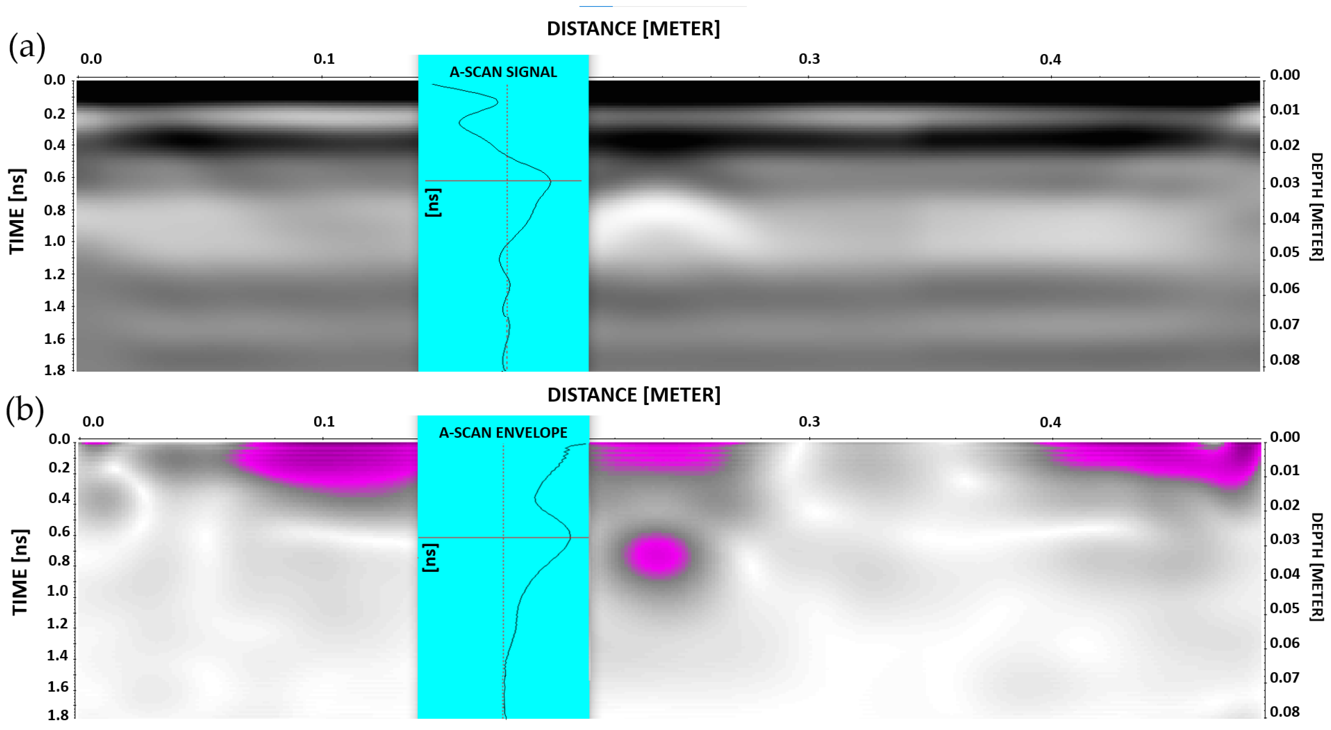
The acquired radargrams were elaborated with Reflex-W [26] by using the Hilbert transform process in order to perform an envelope of the trace amplitudes preserving the signal polarity. It takes the positive and negative components of the signal and collapses them into a total signal that shows the amplitude of that event. All the processed GPR data were exported and analyzed with ad-hoc script permitting to obtain the single traces of the radargram in correspondence to the rebar placed exactly in the middle of the sample. The analyzed traces correspond to the traces at the top of the rebar (Figure 6). The described process allowed us to analyze the variation of the envelope signal in correspondence to the traces on the top of the rebar for the sample immersed in distilled water (“A”), for the sample immersed in water and 5% NaCl (“B”), and for the sample subjected to the accelerated corrosion test (“B”). Therefore, the variations of the envelope signal due to the steel rebar were correlated with the increase of the corrosion phenomena.

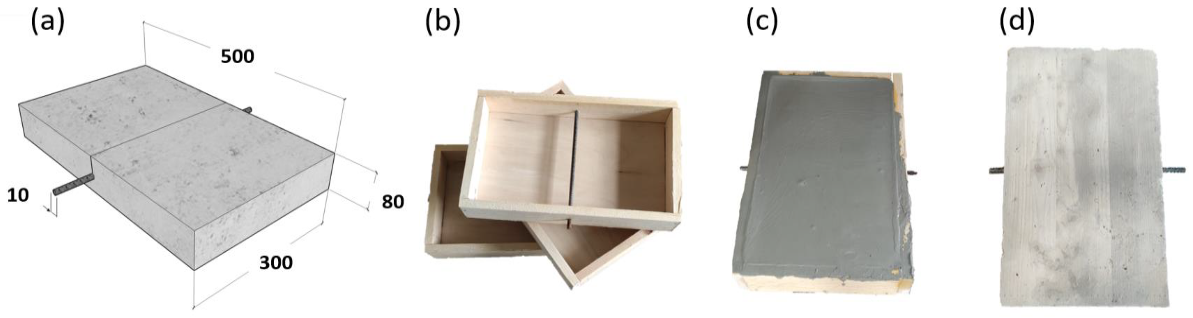
3.1. Sample “A” Immersed in a Distilled Water

In the first phase of this study, a reinforced concrete sample was immersed in a distilled water tank. The experiment was set in order to have a water level of 1cm from the bottom. The water level was kept constant during the investigation period inside the plastic tank with a refilling procedure. After the immersion of the sample in the distilled water tank, the water rose by capillarity within the sample. In order to check this phenomenon, the GPR signals were analyzed each day. After 10 days, the GPR signals were constant due to the stabilization of the humidity inside the concrete sample. We used distilled water so that the corrosion phenomena of the steel rebar inside the concrete sample were inactive or very slow. This first phase of study on the laboratory sample allows us to obtain the envelope signal relating to the wet concrete sample and the steel rebar without the presence of corrosion. The data set of this phase was used to normalize the envelope values obtained in the first tests on the concrete sample immersed in distilled water.

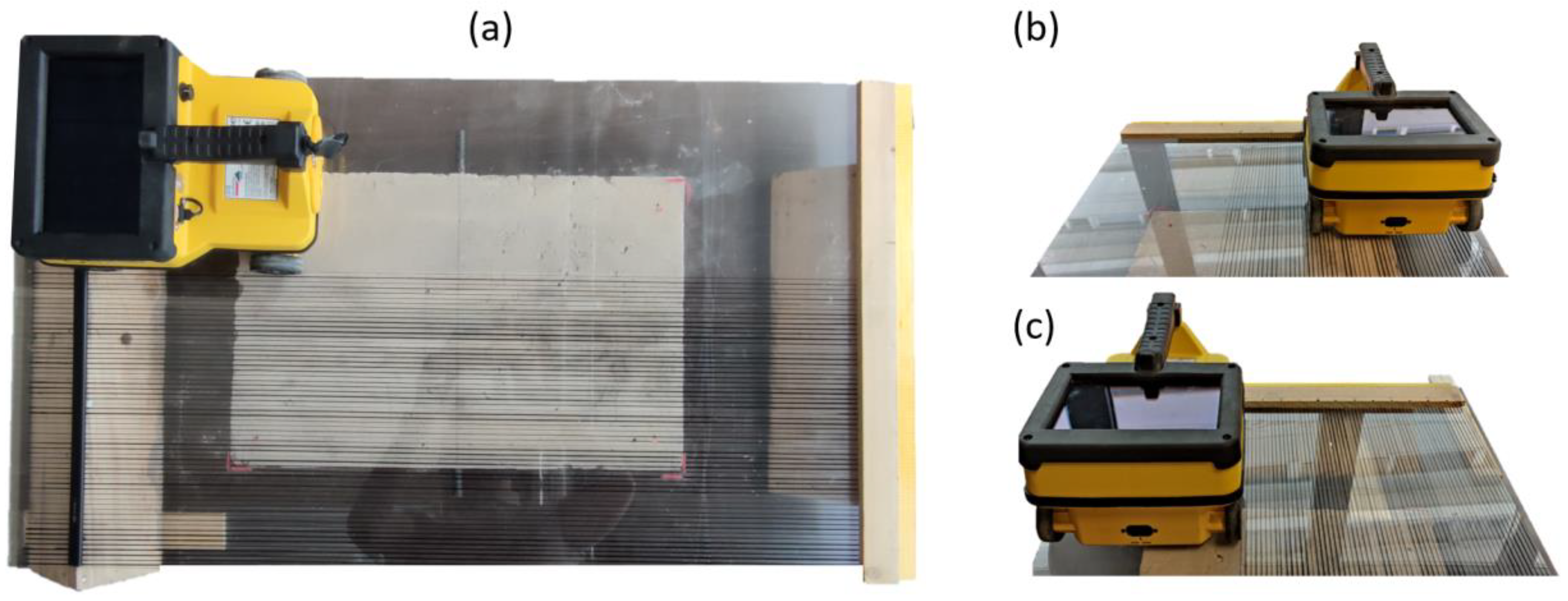
For each day, sixty radargrams were carried out on the sample surface with an interval distance of about 0.5mm following black lines drawn on Plexiglass (Figure 3).

Figure 7 highlights five GPR traces of the envelope process, which have been extrapolated from the same acquired radargram, in the middle of the concrete sample, on 5 different days after the humidity stabilization.

All the identified traces were extracted in the same position where is located the steel rebar, and each one was acquired on different days. The envelope traces at 0.6 ns, where the rebar is located, highlight an envelope value of around 2600, and some variations are identified.

Figure 8 shows the envelope values of each trace acquired in the same position (where the rebar is located) coming from all the parallel radargrams acquired during the fifth day.

3.2. Sample “B” Wet Sample Immersed in a 5% NaCl Water

Sample B was immersed in salt water with 5% of NaCl for one centimeter from the bottom. After 10 days, we started GPR investigations on the concrete samples. The surveys were carried out every 24 h for 5 days; the first survey was identified as T2_1 while the last one was T2_5. Figure 9 highlights the envelope of A scan of the radargram n°29, related to the trace where the steel rebar is located. Even if the surveys were conducted in a similar way to the previous sample “A,” the envelope values at the reinforcement bar, at 0.6 ns, where the steel rebar is located, are greater than in the previous case. Moreover, a small variation of the envelope values is identified.

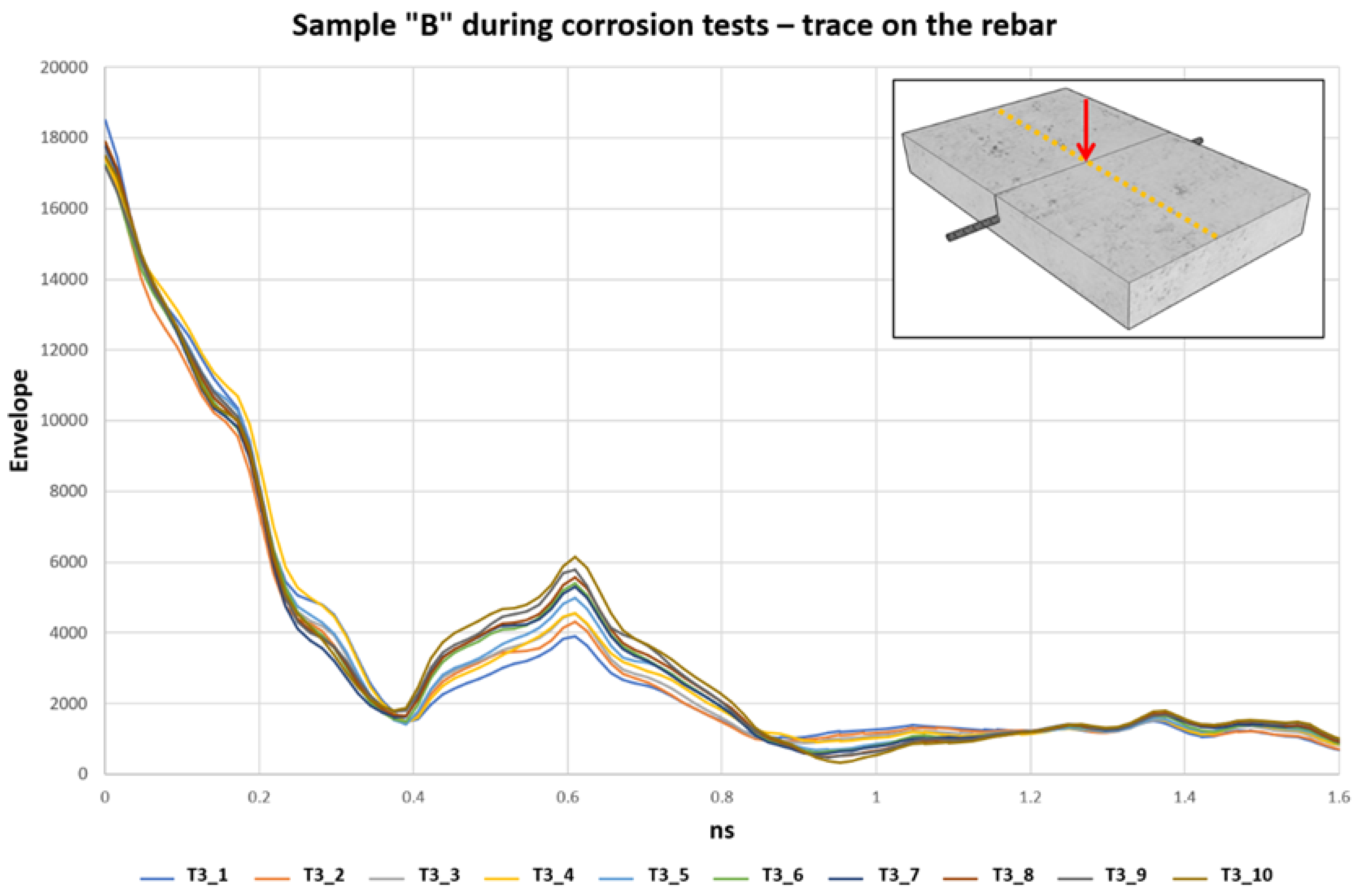
3.3. Sample “B” Wet Sample Immersed in 5% NaCl Water during the Induced Corrosion

After the first phase, sample B was exposed to corrosion by exploiting an external power supply (Hewlett DC). The accelerated corrosion test was carried out by connecting the positive pole of a Hewlett DC power supply to the steel rebar (anode), and the negative pole was connected to a brass bar immersed in the solution of 5% NaCl and 95% of water. The DC power supply has established a potential difference of 25.0 V. The corrosion current in the initial phase was 0.4 A, then gradually lowered to the minimum value of 0.08 A. It was not possible to set a constant current throughout. 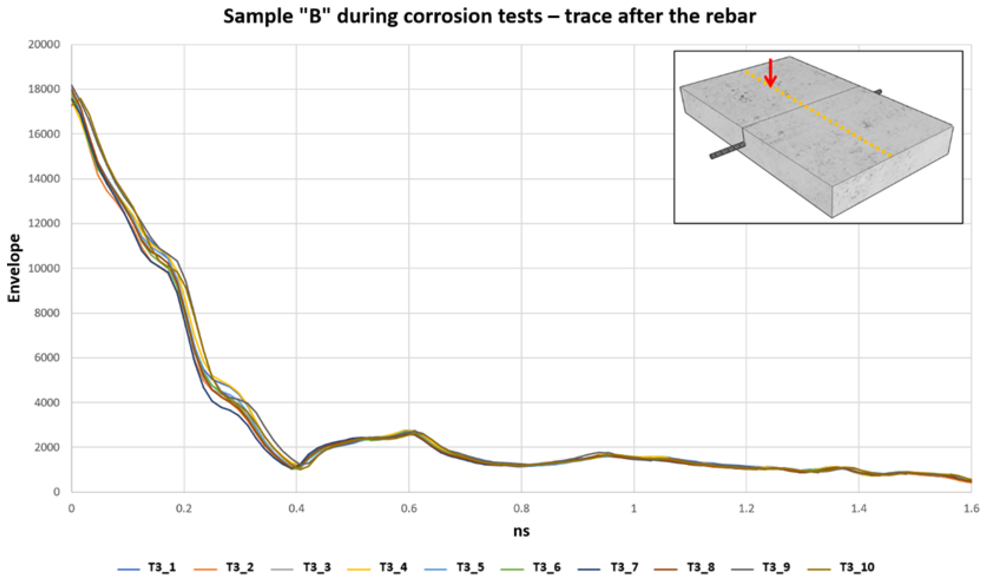Figure 10 shows the increase of the envelope trace obtained every 24 h, starting from the minimum value on the first day (T3_1) and reaching the maximum value after 10 days (T3_10). Investigations with the GPR were carried out each day. The traces in Figure 9 come from the radargram n°29, at the midpoint of the sample, where the rebar is located. During the corrosion test, an increase in the envelope signal was recorded at the trace above the reinforcement bar. The signal initially had a value of 3913 which gradually increased every day and reaches its maximum peak of 6147 on the last day of monitoring performed. The monitoring after 10 days was stopped as we arrived at the complete rupture of the steel rebar.

In order to compare the increase in the envelope signal close to the reinforcement bar, associated with oxidation and consequent corrosion of the rebar, an envelope A-scan trace of the same radargram (n°29) but localized far from the steel rebar, was analyzed. Figure 11 and Figure 12 highlight the trend during the accelerated corrosion test.

The trace acquired during the different days and localized far from the rebar position showed any change in the envelope signal during the corrosion test. The traces away from the reinforcement steel rebar remain unchanged. Consequently, there were any variations in the characteristics of the concrete during the corrosion test. The changes in the envelope signal are limited to the area where the steel reinforcement bar is located. The traces above the reinforcement steel rebar show an increase in the envelope signal during the corrosion test (Figure 11).

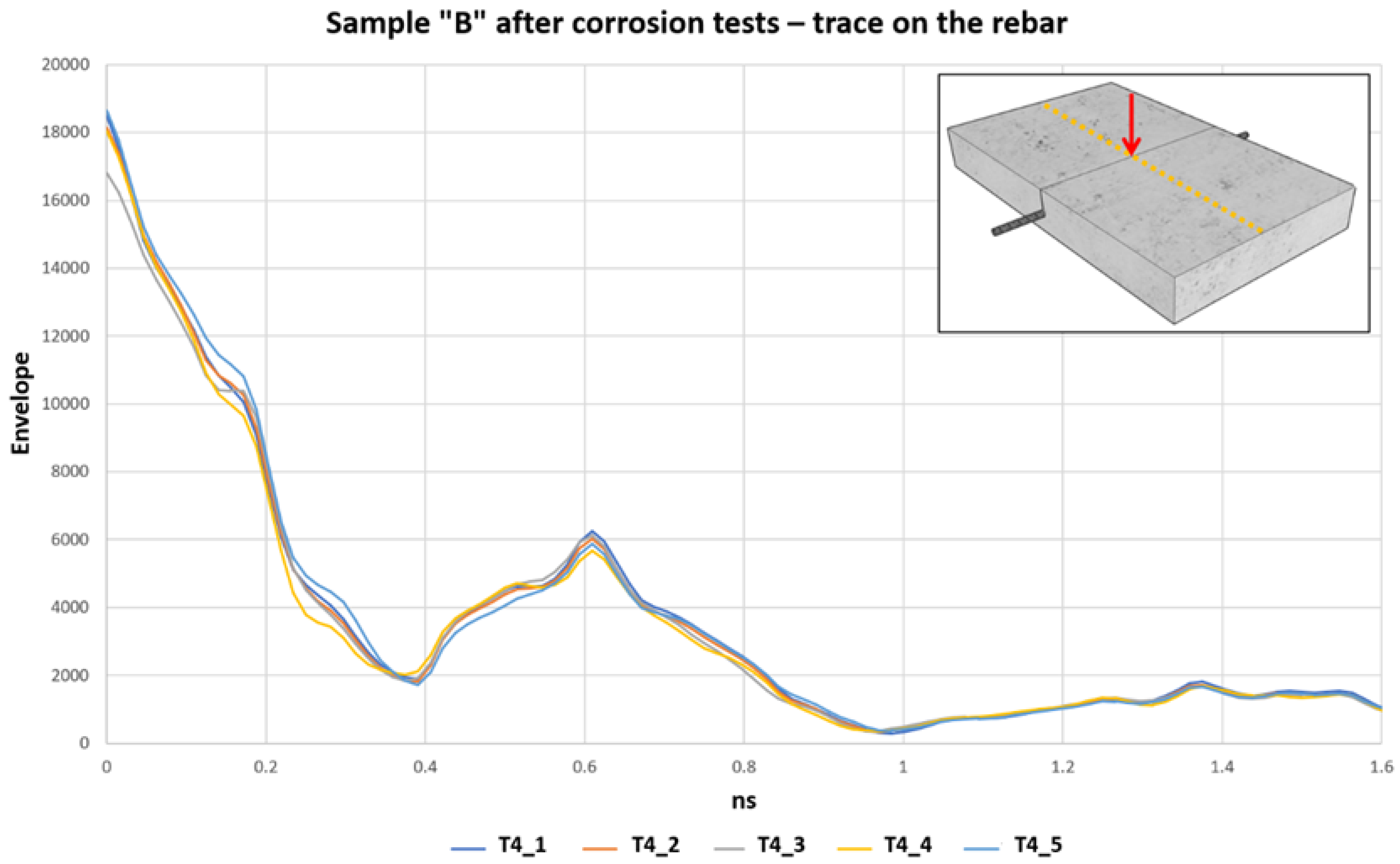
3.4. Sample “B” Wet Sample after Corrosion Tests

After 10 days of accelerated corrosion test, a small fracture was observed at the upper side of the sample. Therefore, the injection of the current was stopped. After the current stop phase, for 5 days, new acquisitions were carried out to observe the values of the envelope signal around the steel rebar. The investigations carried out at this stage are indicated with T4. They were performed every day, and each one is shown in Figure 13 as T4_1, T4_2, T4_3, T4_4, and T4_5. The acquisitions were always carried out as the previous ones. Figure 12 shows the A-scan envelope signal acquired above the reinforcement steel rebar and at 0.6 ns, where it is located the steel rebar. The data highlights an unchanged envelope during the five days after the corrosion test.

The value reached in the T3_10 survey, during the corrosion tests, in the envelope A-scan on the steel rebar was 6147, and it was the maximum value reached during all the experiments.

3.5. Self-Potential Acquisition and Elaboration

Self-potential investigations were carried out on the reinforced concrete sample before starting the accelerated corrosion tests and at the end of the tests. Indeed, during the induced corrosion, the electrical signals recorded are correlated to the injected current. Moreover, regarding the sample immersed in 5% NaCl water, we waited for the moisture content in the sample to be stable. The stabilization occurred after 10 days, and at this point, we carried out a Self-potential investigation on the sample. The adopted procedure consisted in measuring the electric potential difference between the steel reinforcement rebar and a reference electrode (in our case, we used an unpolarizable lead electrode). The reference electrode was placed directly in contact with the sample surface and connected via the negative cable to a voltmeter, while the reinforcement was connected to the positive pole.

The acquired data have allowed us to map the isopotential lines using the Surfer software (Figure 14). The isopotential lines are able to define the presence of corrosion phenomena in progress at the time of the measurement. In our case, the higher potential values are correlated with the corrosion phenomena in progress at the time of the measurement. The colour scale used ranges from white to red, white for low potential values and red for high potential values. The isopotential maps acquired at the end of the induced corrosion experiment show two areas coloured in red (high potential) that should be associated with the higher corroded zone. These areas highlight SP values > 300 mV, while the isovalues obtained before the induced corrosion phase show a potential value < 200 mV.

4. Discussion

In this paper, the geophysical acquisitions, GPR and Self-Potential, were carried out on two identical reinforced concrete samples with the aim of investigating the corrosion of the steel bars. The concrete samples were investigated with a 2 GHz antenna, and the data processing was characterized by applying the Hilbert Transform with the Envelope filter. The elaborated A-scan traces were analyzed during the induced corrosion phenomena, and a good correlation between the increase of the envelope signal and the corrosion of the reinforcement steel rebar was detected. The experiments on the concrete samples were carried out under different scenarios. The samples were partially immersed in water, one in distilled water (Sample A) and one with a content of 5% of NaCl (Sample B). Sample A has been taken as a reference to having indications relating to the envelope signal of the wet sample without the presence of corrosion. Once this reference was obtained, we had the opportunity to compare the investigations conducted on sample B, in this case, with the presence of corrosion phenomena in progress. In fact, sample B was partially immersed in saline water, and as soon as it was immersed in water, the chlorides present in the solution began to rise inside the sample, activating the depassivation processes of the steel rebar.

On both samples, we organized a series of surveys carried out as monitoring; every 24 h, a survey was carried out using the GPR with a central frequency of 2 GHz band. All the A-Scan traces were analyzed by applying the Hilbert Transform through the envelope filter. The study took into consideration the traces above the reinforcement bar as they are of interest to us for the observation of corrosion phenomena.

In the first phase, the A-Scan track defined the depth at which the reinforcement bar was located. After the identification of the reinforcement bar, the envelope of the corresponding trace was calculated, and its variation was monitored for the entire laboratory test. The envelope values obtained on sample A are roughly constant in the time, and the average, obtained from the data acquired in correspondence with the steel rebar, is around 2600. This behaviour should be correlated with an equilibrium between the constant value of the water content in the concrete and the absence of corrosion during the acquisition time.

In the first phase of the investigations on sample B, during the pre-induced corrosion phase, the envelope values highlighted a small variation in the time but with an increase of them compared with the data acquired on sample A, immersed in distilled water. The envelope values measured in correspondence of the steel rebar on sample “B” were around 3800. Therefore, this increase should be associated with corrosion which took place in a natural way and was not induced by the test. The chlorides inside the solution immediately activated the corrosion processes, and the steel rebar began to oxidize. This is confirmed by the investigations carried out with the self-potential method, which showed very high values from the first day of testing. The onset of the corrosion was also visible where the bar was exposed.

In order to compare the results obtained before the induced corrosion phase, the average of the envelope values coming from each parallel radargram is plotted in Figure 15. These envelope values are extracted from each trace obtained on the same position of all parallel radargrams. The used traces are located in correspondence with the steel rebar. The blue ones are the envelope values applied on the radargram carried out on Sample A, and the orange ones come from the data set acquired on Sample B.

The histograms show the numbers of the radargram and the envelope values. The histogram bars represent the average envelope value extracted at 0.6 ns, that is, the TWT associated with the location of the steel bar.

The envelope values are obtained by applying the Hilbert transform to the radargrams from n°5 to n°55. Only the odd radargrams are plotted to simplify the visibility of the graph. The trend of the histogram bars highlights several peculiarities. An increase in envelope values is well identified on the lateral sides of the two samples (before the radargram n°17 and after n°43). This lobe shape is well identifiable on all the radargrams; therefore, it should be associated with lateral effect due to the dimension of the used antenna. Therefore, in the next consideration, it is necessary to take into account this lateral effect. Anyway, the histogram related to sample “B” shows an average of the envelope values greater than the survey carried out at the same time on sample “A.” Therefore, these differences should be associated with an activation of the corrosion faster in sample B, which was submerged in water with 5% NaCl, than in sample A, where the water was distilled.

When the induced corrosion was applied to sample B, a gradual increase in the envelope values at 0.6 ns of the trace, where is located the reinforcement bar, was well depicted (Figure 13). The monitoring was carried out every 24 h, and the investigations were carried out by switching off the power supply, which allows us to carry out the corrosion of the steel rebar. The next step consisted of extracting the filtered data in the same time position (0.6 ns) and plotting all of them. An important trend was observable. In general, there was a positive trend in the envelope values, from a minimum of 3800 up to 6147. In detail, the increase of the envelope values was not the same everywhere. There are areas along the steel rebar where the elaborated signals increase more than in other sites. This effect is well identified in Figure 16, where a histogram plots the envelope variations in each radargram position at different times. Each colour corresponds to the same time acquisition. Ten acquisition days were defined, making induced corrosion phenomena in sample B. Therefore, ten radargrams were carried out on each selected line in order to obtain n.550 enveloped values along the steel rebar.

The lateral effects described before are still highlighted, where two main lobes are defined. During the injected current phase, two periods (days 2 and 3) show a large increase in the envelope values enough everywhere. The days after the increment decreased but with a large difference from different sites. From a site location point of view, a large relative increment of the envelope values is well-identified close to the lateral part of the sample. This behavior should be associated with greater corrosion of the steel rebar at the border of the sample with respect to the central part. This interpretation is also confirmed by the Self-Potential data set. Figure 14 shows the acquired potential data acquired at the end of the induced corrosion phase (day 10). Higher values are well identified on the lateral side of the sample, in correspondence with the two lobes are observed on the histograms and defined by the acquired envelope values. Therefore, the injected current induced faster corrosion in these areas where the oxide production increased. This hypothesis was also confirmed because the iron oxides were well identified on the later side of the sample where the iron bar is visible.

After the accelerated corrosion phase, the power supply was turned off. At this moment, the last acquired phase started with new GPR acquisitions and lasted for another five days. The elaborated data show a small variation of the envelope values during the five days. Small variations (increments and decrements) were observed (Figure 13). This behavior highlights a good correlation between the envelope data and the corrosion process with the production of iron oxide. Therefore, when the induced corrosion was stopped, also the deposition of dust material decreased around the non-corroded steel.

In order to observe the variation of the envelope value due to the induced corrosion, the maximum envelope value reached during the end of the second phase (induced corrosion experiment) was normalized with the average value of each trace obtained during the first phase. This approach permitted the observation of only the envelope increase due to corrosion phenomena, excluding the side effect (Figure 17). The obtained histogram highlights different increments of the envelope values along the steel bar: strong envelope values are located on the two lateral zones and a slight increase in the centre of the reinforcement bar.

The SP map acquired at the end of the induced corrosion phase depicted two main areas with a high probability of corrosion. These two areas are located close to the border of the sample, where two large increments of envelope values are identified. Figure 17 shows the histogram of the normalized envelope values obtained at the end of the induced corrosion phase on the SP map, highlighting very well the previous discussion. Therefore, integrating the SP approach and the GPR investigations, the corrosion phenomena should be observed, and the areas in correspondence with the reinforcing steel rebar where there is corrosion should be detected. At the end of the experiments, the sample was broken to have a visual analysis of the corroded zone close to the rebar (Figure 18). In order to understand the relationship between the envelope signal and the corrosion of the steel rebar, we decided, at the end of the tests carried out, to break the concrete sample on the steel rebar. Comparing the histogram plot and the picture of the broken sample, large areas with the dust of the corroded steel rebar are visible, and a good correlation should be observed with the envelope values.

5. Conclusions

The paper introduces a non-destructive method oriented to the qualitative and quantitative assessment of the progress of the corrosion process of RC structures. The study analyzed laboratory investigations on reinforced concrete structures by GPR and Self-potential methods. The GPR is one of the NDT methods with several advantages over other methods for RC characterization and monitoring. It could examine large areas in a short time, providing information on the depth and spacing of rebars. Several papers identified the GPR as a challenging method for corrosion assessment. Previous studies have reported in the literature on the correlation between the GPR signal amplitude and the presence of corrosion, but opposing results were observed. This paper introduces a novel approach to observing the corrosion phenomena exploiting the contribution of the Hilbert transform for the analysis of GPR data. Results have demonstrated that the changes in the envelope values could be imputable to the rebar corrosion. Further, the obtained results with GPR show a good agreement with the ones provided by the self-potential method. The results also showed that the GPR could directly detect the degree of corrosion of rebar located in concrete structures, which was also observed by the self-potential data set. The obtained results will address the next steps of our research introducing samples with an increase in the number of rebars and more complex rebar configurations, simulating real-life scenarios. This approach will trigger the best GPR analysis on the rebar corrosion processes in real-life structures. Anyway, on-site in real conditions, several factors influence the GPR response, such as moisture and chloride content, which make the detection of corroded zones based on the observation of GPR potentially ambiguous. The detection of other variables imputable to the corrosive environment hosting the steel rebar needs to be detected. Even if the effect of the corrosion on the GPR signal is well identified for the investigated samples, the use of various geophysical techniques is warmly recommended during laboratory experiments. Moreover, to obtain maximum knowledge about the rebar corrosion state in real-life structures, a combination of measuring techniques with a multisensor approach (i.e., SP, DC, IP, IRT, US) will be the future field setting [32].

References

1. Daniyal, M.; Akhtar, S. Corrosion assessment and control techniques for reinforced concrete. J. Build. Pathol. Rehabil. 2020, 5, 1. [Google Scholar] [CrossRef]
2. Bossio, A.; Monetta, T.; Bellucci, F.; Lignola, G.P.; Prota, A. Modeling of concrete cracking due to corrosion process of reinforcement bars. Cem. Concr. Res. 2015, 71, 78–92. [Google Scholar] [CrossRef]
3. Tešic’, K.; Baricevic, A.; Serdar, M. Non-Destructive Corrosion Inspection of Reinforced Concrete Using Ground-Penetrating Radar: A Review. Materials 2021, 14, 975. [Google Scholar] [CrossRef] [PubMed]
4. Verma, S.K.; Bhadauria, S.S.; Akhtar, S. Monitoring Corrosion of Steel Bars in Reinforced Concrete Structures. Sci. World J. 2014, 2014, 957904. [Google Scholar] [CrossRef] [PubMed]
5. Capozzoli, L.; Rizzo, E. Combined NDT techniques in civil engineering applications: Laboratory and real test. Constr. Build. Mater. 2017, 154, 1139–1150. [Google Scholar] [CrossRef]
6. Tosti, F.; Alani, A.M.; Benedetto, A. Guest Editorial: Recent Advances in Non-destructive Testing Methods. Surv. Geophys. 2020, 41, 365–369. [Google Scholar] [CrossRef]
7. Capozzoli, L.; Fornasari, G.; Giampaolo, V.; De Martino, G.; Rizzo, E. Multi-Sensors Geophysical Monitoring for Reinforced Concrete Engineering Structures: A Laboratory Test. Sensors 2021, 21, 5565. [Google Scholar] [CrossRef]
8. Fornasari, G.; Capozzoli, L.; De Martino, M.; Giampaolo, V.; Rizzo, E. Rebar Corrosion Monitoring with a Multisensor Non-Destructive Geophysical Techniques. In Proceedings of the 45th International Conference on Telecommunications and Signal Processing (TSP), Prague, Czech Republic, 13–15 July 2022; pp. 367–370. [Google Scholar] [CrossRef]
9. Ohtsu, M. Introduction. In Innovative AE and NDT Techniques for On-Site Measurement of Concrete and Masonry Structures; Springer: Dordrecht, UK, 2016; Volume 20, pp. 1–4. [Google Scholar]
10. Hubbard, S.S.; Zhang, J.; Monteiro, P.J.M.; Peterson, J.E.; Rubin, Y. Experimental Detection of Reinforcing Bar Corrosion Using Nondestructive Geophysical Techniques. ACI Mater. 2003, 100, 501–510. [Google Scholar] [CrossRef]
11. Hong, S.; Lai, W.W.L.; Wilsch, G.; Helmerich, R.; Helmerich, R.; Günther, T.; Wiggenhauser, H. Periodic mapping of reinforcement corrosion in intrusive chloride contaminated concrete with GPR. Constr. Build. Mater. 2014, 66, 671–684. [Google Scholar] [CrossRef]
12. Hong, S.; Lai, W.W.L.; Helmerich, R. Experimental monitoring of chloride-induced reinforcement corrosion and chloride contamination in concrete with ground-penetrating radar. Struct. Infrastruct. Eng. 2015, 11, 15–26. [Google Scholar] [CrossRef]
13. Tesic, K.; Baricevic, A.; Serdar, M.; Gucunski, N. Characterization of ground penetrating radar signal during simulated corrosion of concrete reinforcement. Autom. Constr. 2022, 143, 104548. [Google Scholar] [CrossRef]
14. Lai, W.W.L.; Kind, T.; Stoppel, M.; Wiggenhauser, H. Measurement of Accelerated Steel Corrosion in Concrete Using Ground Penetrating Radar and a Modified Half-Cell Potential Method. J. Infrastruct. Syst. 2013, 19, 205–220. [Google Scholar] [CrossRef]
15. Chang, C.W.; Tsai, C.A.; Shiau, Y.C. Inspection of Steel Bars Corrosion in Reinforced Concrete Structures by Non-destructive Ground Penetrating Radar. Appl. Sci. 2022, 12, 5567. [Google Scholar] [CrossRef]
16. Wong, P.T.W.; Lai, W.W.L.; Sham, J.F.C.; Poon, C. Hybrid non-destructive evaluation methods for characterizing chloride-induced corrosion in concrete. NDT E Int. 2019, 107, 102123. [Google Scholar] [CrossRef]
17. Jin, L.; Liu, M.; Zhang, R.; Du, X. Cracking of cover concrete due to non-uniform corrosion of corner rebar: A 3D meso-scale study. Constr. Build. Mater. 2020, 245, 118449. [Google Scholar] [CrossRef]
18. Song, H.W.; Saraswathy, V. Corrosion Monitoring of Reinforced Concrete Structures—A Review. Int. J. Electrochem. Sci. 2007, 2, 1–28. [Google Scholar]
19. Zaki, A.; Johari, M.A.M.; Hussin, W.M.A.W.; Jusman, Y. Experimental assessment of rebar corrosion in concrete slab using Ground Penetrating Radar (GPR). Int. J. Corros. 2018, 2018, 5389829. [Google Scholar] [CrossRef]
20. Sossa, V.; Perez-Gracia, V.; Gonzalez-Drigo, R.; Rasol, M.A. Lab non-destructive test to analyze the effect of corrosion on ground penetrating radar Scans. Remote Sens. 2019, 11, 2814. [Google Scholar] [CrossRef]
21. Agred, K.; Klysz, G.; Balayssac, J.P. Location of reinforcement and moisture assessment in reinforced concrete with a double receiver GPR antenna. Constr. Build. Mater. 2018, 188, 1119–1127. [Google Scholar] [CrossRef]
22. Tarussov, A.; Vandry, M.; De La Haza, A. Condition assessment of concrete structures using a new analysis method: Ground penetrating radar computer-assisted visual interpretation. Constr. Build. Mater. 2013, 38, 1246–1254. [Google Scholar] [CrossRef]
23. Hasan, M.I.; Yazdani, N. An Experimental Study for Quantitative Estimation of Rebar Corrosion in Concrete Using Ground Penetrating Radar. J. Eng. 2016, 2016, 8536850. [Google Scholar] [CrossRef]
24. Liu, H.; Zhong, J.; Ding, F.; Meng, X.; Liu, C.; Cui, J. Detection of early-stage rebar corrosion using a polarimetric ground penetrating radar system. Constr. Build. Mater. 2022, 317, 125768. [Google Scholar] [CrossRef]
25. Zatar, W.; Nguyen, T.T.; Nguyen, H. Environmental effects on condition assessments of concrete structures with ground penetrating radar. J. Appl. Geophys. 2022, 203, 104713. [Google Scholar] [CrossRef]
26. Sandmeier, K.J. ReflexW Version 8.1. Program for Processing of Seismic, Acoustic or Electromagnetic Reflection, Refraction and Transmission Data; Software Manual: Karlsruhe, Germany, 2016; 628p. [Google Scholar]
27. Dinh, K.; Gucunski, N.; Kim, J.; Duong, T.H. Understanding depth-amplitude effects in assessment of GPR data from concrete bridge decks. NDT E Int. 2016, 83, 48–58. [Google Scholar] [CrossRef]
28. Rodrigues, R.; Gaboreau, S.; Gance, J.; Ignatiadis, I.; Betelu, S. Reinforced concrete structures: A review of corrosion mechanisms and advances in electrical methods for corrosion monitoring. Constr. Build. Mater. 2021, 269, 121240. [Google Scholar] [CrossRef]
29. Pour-Ghaz, M.; Isgor, O.B.; Ghods, P. Quantitative interpretation of half-cell potential measurements in concrete structures. J. Mater. Civ. Eng. 2009, 21, 467–475. [Google Scholar] [CrossRef]
30. ASTM C876-91; Standard Test Method for Half-Cell Potentials of Uncoated Reinforcing Steel in Concrete. ASTM International: West Conshohocken, PA, USA, 1999.
31. ASTM C876-15; Standard Test Method for Corrosion Potentials of Uncoated Reinforcing Steel in Concrete. ASTM International: West Conshohocken, PA, USA, 2015.
32. Solla, M.; Lagüela, S.; Fernández, N.; Garrido, I. Assessing Rebar Corrosion through the Combination of Nondestructive GPR and IRT Methodologies. Remote Sens. 2019, 11, 1705. [Google Scholar] [CrossRef]
Figure 1. (a) GPR acquisition on corroded rebar in concrete; (b) radargram acquired along the concrete sample, the hyperbola corresponds to corroded rebar.
Remotesensing 15 02206 g001
Figure 2. Reinforced concrete laboratory sample; (a) project of the realized concrete sample and dimension; (b) wooden formwork for the construction of the sample; (c) sample construction; (d) completed reinforced concrete sample.
Remotesensing 15 02206 g002
Figure 3. Accelerated corrosion tests with the impressed current technique. (a) The reinforced concrete sample was immersed in a solution of 5% NaCl and 95% of water. (b) the used Hewlett DC Power supply.
Remotesensing 15 02206 g003
Figure 4. GPR acquisition system and the plexiglass plane where several lines were depicted in order to make all the radargrams in the same position. (a) Image from the top; image from behind the antenna where the first (b) and the last (c) profiles were carried out.
Remotesensing 15 02206 g004
Figure 5. Acquisitions of Self-Potential (SP) on the reinforced concrete sample.
Remotesensing 15 02206 g005
Figure 6. One of the radargrams was acquired at the center of the concrete sample. (a) the radargram highlights the amplitude of the em signal in correspondence to the steel rebar. (b) The envelope filter has been applied to the radargram.
Remotesensing 15 02206 g006
Figure 7. Envelope A-scan acquired on the sample “A.” The trace shown is taken from radargram 29, which is exactly in the middle of the concrete sample. The track considered is above the steel rebar present at 0.6 ns. The trace remains constant during the 5 days of investigation, T1_1 at T1_5.
Remotesensing 15 02206 g007
Figure 8. Histogram of the envelope signal at the steel rebar for the radargrams acquired on the concrete sample. The value shows the envelope value on the steel rebar at 0.6 ns time depth.
Remotesensing 15 02206 g008
Figure 9. Envelope A-scan acquired on sample “B.” The trace shown is taken from radargram 29, which is exactly in the middle of the concrete sample. The track considered is above the steel rebar present at 0.6 ns. The trace remains constant during the 5 days of investigation, T2_1 at T2_5.
Remotesensing 15 02206 g009
Figure 10. Envelope A-scan was acquired on sample “B” during the accelerated corrosion test. The trace shown is taken from radargram 29, which is exactly in the middle of the concrete sample. The track considered is above the steel rebar present at 0.6 ns.
Remotesensing 15 02206 g010
Figure 11. Envelope A-scan was acquired on sample “B” during the accelerated corrosion test. The trace shown is taken from radargram n°29, at 10 cm after steel rebar, inside the concrete sample. From the graph, we can see that there were no changes in the envelope A-scan trace during the corrosion test.
Remotesensing 15 02206 g011
Figure 12. Envelope A-scan was acquired on sample “B” during the accelerated corrosion test. The trace shown is coming from the radargram n°29, 10 cm before the steel rebar. From the graph, we can see that there were no changes in the envelope A-scan trace during the corrosion test.
Remotesensing 15 02206 g012
Figure 13. Envelope A-scan was acquired on sample “B” after an accelerated corrosion test. The trace shown is taken from radargram 29 on the steel rebar.
Remotesensing 15 02206 g013
Figure 14. Self-potential maps were obtained on the concrete sample. The map shown on the left was realized the day before starting the accelerated corrosion tests on the sample. The map on the right was obtained after 10 days of accelerated corrosion testing.
Remotesensing 15 02206 g014
Figure 15. Envelope values along the steel rebar for sample “A” (top) and for sample “B” (bottom). Each bar of the histogram represents the average value of the envelope signal applied on all the radargrams acquired before the induced corrosion phase. Only the odd radargrams were plotted from n°5 to n°55.
Remotesensing 15 02206 g015
Figure 16. Envelope values along the steel rebar for sample “B” during the accelerated corrosion tests for ten days of monitoring. The investigation at T3_1 was carried out after 24 h, switching on the power supply, and subsequent surveys, every 24 h.
Remotesensing 15 02206 g016
Figure 17. The histogram depicts the maximum envelope value reached for each trace at T3_10 normalized with respect to the average of the traces acquired during the first phase (T1).
Remotesensing 15 02206 g017
Figure 18. The picture of the broken sample in correspondence of the steel rebar with the histogram of the normalized envelope values and the self-potential profile along the sample.
Remotesensing 15 02206 g018