A Comparison of Seven Medium Resolution Impervious Surface Products on the Qinghai–Tibet Plateau, China from a User’s Perspective

Abstract

As a vital land cover type, impervious surface directly reflects human activities and urbanization, significantly impacting the environment, climate, and biodiversity, especially in ecologically fragile areas such as the Qinghai–Tibet Plateau (QTP) in China. Thus, precise knowledge of impervious surface information on the QTP is essential for its ecological protection and social development. In order to improve the application of products and inform further studies, we assessed the accuracy of seven medium resolution (10–30 m) impervious surface products in the QTP, including GAIA, CISC, GlobalLand30 (GL30), GLC-FCS30 (FCS30), GHS-BUILT-S2 (GHSB), ESA WorldCover10 (WC10), and Dynamic World NRT products (DW). The validation set labeled according to domestic GF-1 images was used to calculate the precision, recall, and F1-Score of these products, and two impervious surface vote maps were generated to analyze their spatial consistency. The results showed that CISC and DW had the highest overall quality among the 30 m and 10 m products, with F1-Scores of 0.5701 and 0.5670, respectively. We also validated the accuracy of different data combinations and their intersection and union sets to provide guidance based on the results for data selection in impervious surface studies on the QTP. For results calculated by the strict validation set, which was exclusive of mixed grids, precision decreased slightly while recall increased significantly for all products, indicating that the omissions were mostly mixed pixels with a smaller percentage of impervious surface. In terms of spatial consistency, the maximum impervious surface range voted by the seven products jointly only accounts for 0.82% of the QTP, which is 2,786,800 km² in total. Additionally, the high consistency area (votes > 4), with a distribution concentrated in large cities and dense buildings, only accounts for 15.18% of this maximum range. In summary, each product’s regional accuracy in the QTP was lower than their published accuracy, and they omitted many impervious surfaces, especially those with a background of bare land.

1. Introduction

Impervious surfaces are a critical artificial surface type. On the one hand, they change the process of rainwater runoff, infiltration, and surface evapotranspiration, which directly affects the regional environment, ecology, biodiversity, and disaster occurrence [1,2,3]; on the other hand, they are a direct reflection of human activities, whose distribution, expansion, and evolution indicates the development of cities and population flows [4,5,6], making it an essential data reference for studies on urban heat islands [7], carbon emissions [8], urban and regional planning [9], and urban management. As “the third pole of the world” [10,11], the Qinghai–Tibet Plateau (QTP) is an important global ecological security barrier, even limited human activities there may bring about significant changes to the global ecology, climate, and environment [12,13,14]. Atmospheric circulation models have suggested that the changes in land use, in which urbanization is a factor, caused by the rapid growth of human activities over the past half-century, led to significant temperature increases on the QTP [15]. Ecosystem damages caused by human activities weaken ecosystem services, negatively affecting the ecological security barrier function of the QTP [16]. Many studies have been devoted to unraveling the patterns of the impact of human activities on the ecological environment, such as human footprint studies [17,18], in which the impervious surface product is vital input data. Moreover, the QTP accounts for about one quarter of China’s total land area (9.6 million km²). Accurately quantifying the area and distribution of artificial impervious surfaces on the QTP is one of the critical elements of national land surveys and land supervision [19], as well as an essential data reference for guiding the construction of sustainable cities in the QTP region. Furthermore, the low density of impervious surfaces, the frequent cloud cover, and the bare ground background make impervious areas in the QTP more complicated. At the same time, it is because of the small size of impervious surfaces in the QTP that the overall accuracy evaluation of products on a national or global scale cannot reveal the performance of algorithms in these challenging areas. Namely, for a comprehensive assessment of algorithm capability, it is also vital to conduct an accuracy validation in the QTP. With the development of sensor technology and the construction and upgrading of Earth observation systems in various countries [20,21,22,23], the level of available remote sensing has increased significantly. The spatial resolution of remote sensing images has also developed towards finer scales, such as meters and submeters. Moreover, impervious surface research in the Qinghai–Tibet Plateau based on fine spatial scales has become an urgent requirement [24,25], which demands fine-resolution impervious surface imaging products of reliable quality.

The importance of impervious surfaces has caused many scholars to explore this area, and many of these efforts have borne fruitful results. Over the years, many relevant products and land cover products related to impervious surfaces have been released to the public, such as the coarse resolution data MODIS Land Cover (2001–2020) at 500 m; for 30 m resolution products, the global impervious surface dynamic datasets GAIA (1985–2018) [26] and GISD30 (1985–2020) [27], the global artificial impervious surface map GMIS (2010) [28] and urban map NUACI (1980–2015) [29], and the global land cover data FROM_GLC (2010, 2015) [30] and GlobalLand30 (2000, 2010, 2020) [31] have been released; and the 10 m resolution products include those containing the global built-up area dataset GHS-BUILT-S2 (2018) [32], the global land cover products ESA World Cover (2020) [33], FROM-GLC10 (2017) [34], and the near real-time map Dynamic World V1 shared by Google (2015–present) [35], among others. On the whole, the progress in impervious surface research is following the development of remote sensing technology: the spatial scale of perception has become more refined as the spatial resolution of remote sensing images has increased and the time scale of research findings has evolved from single time series to long time series and high frequencies with the abundance of remote sensing data. The multitudinous data dazzle users and raise new questions: which product is more accurate for impervious surface information in the QTP study area? How consistent are the different products? Due to differences in data sources, extraction algorithms, application objectives, classification system standards, and definitions of classes, the quality of data from different products varies. Meanwhile, the accuracy references provided by existing products mainly consist of overall accuracy, user accuracy, and producer accuracy, as calculated by the validation set. The following three reasons make it difficult to answer the above two questions:

• Validation accuracy is closely related to the validation set being used: the accuracy assessment results may be different when they are calculated by a validation set with different magnitudes or different sampling strategies. Additionally, it is certainly the case that each product has an exclusive validation set. So, it is unreasonable to judge the data quality solely by comparing the absolute value of overall accuracy or category accuracy;
• Validation accuracy is highly correlated with the spatial scale: the accuracy will change with the spatial scale. Namely, the accuracy calculated based on a certain validation set can only measure the overall quality level of the sampling range to which the validation set belongs, rather than the quality of any local area. Common large-scale products often provide the accuracy calculated based on global, continental or national calculations, and for the above reason, this accuracy was unable to reflect the quality in a subset area or a highly heterogeneous region. The QTP is one such place that often has a lower regional accuracy than overall accuracy because of its complex topography, characteristic climatic conditions and lack of available images that are cloud-free or have minimal clouds;
• Discrepancy in choices of validation metrics or deficiency of accuracy assessment information [36,37]: Some existing products do not provide accurate information for specific years, used different validation metrics in the assessment process, or the choices of these metrics were not suitable or too few. For instance, GlobalLand30 only provided overall accuracy without precision and recall of category, and GAIA only assessed the data accuracy in seven representative years, but other years’ accuracies were unknown. This makes it difficult for the user to understand the product quality directly from the data publisher.

Therefore, a comprehensive comparison of different products’ accuracies and an analysis of the consistency of their extraction results in the QTP region have a guiding significance for data selection, application and integration. Many researchers have already carried out related work, such as verifying a single dataset to a specific region [38,39], evaluating multiple products comparatively [40,41,42,43,44,45,46] or validating the new data against other existing products when it was mapped [26,27,28,29,30,31,32,47,48,49]. Moreover,

Table 1. Validation samples details and accuracy results of the product series used in this paper in previous studies.

Study	Region	Validation Samples Description	Accuracy Description
Xing et al. [38]	Beijing, China	The validation set was generated from social media point of interest (POI) data via modified decision trees.	The validation accuracy of artificial surfaces in GL30 in 2010 in Beijing is 92.82%.
Yang et al. [47]	Kuala Lumpur, Malaysia, and its surrounding areas	15 land investigation points and 1635 validation points were obtained via stratified random sampling with the strata of non-urban/urban land and was interpreted based on HR image.	The overall accuracy (OA) of GL30 2010 is 80.54%.
Zhang et al. [48]	Shaanxi, China	The validation set was generated using an augmented sampling method without violating the principles of stratified sampling, containing a shared subset for all products and a separate one for individual products. Concretely, there were 712 and 703 samples for GL30 in 2010 and 2020 and 705 and 699 samples for FCS30 in 2010 and 2020.	The OA of GL30, FCS30 is 80.80%, 75.33% in 2010 and 78.41%, 79.41% in 2020; the user accuracy (UA) of artificial surfaces in GL30, FCS30 is 61.54%, 86.27% in 2010 and 66.04%, 86.79 in 2020.
J. Wang et al. [40]	The southwest of China	3113 samples from the Geo-Wiki Global Validation Sample Set (Geo-Wiki); 488 samples from the Global Land Cover Validation Sample Set (GLCVSS) and 4606 samples from visual interpretation (VI).	The overall accuracy of WC10 2020 is 45.13%, 54.92%, and 64.50%, respectively, calculated by Geo-Wiki, GLCVSS, and VI, with the kappa is 0.314, 0.42 and 0.58; The UA of “built up” is 73.17%, 50% and 94.57% and the producer accuracy (PA) of “built up” is 65.22%, 50% and 74.49, correspondingly.
Huang et al. [49]	Global	39,477 impervious surface area samples and 79,345 non-impervious surface samples were extracted from the ZiYuan-3 global built-up dataset and visually inspected.	The OA of GAIA is 87.91%; the UA and PA of impervious surfaces are 80.98% and 83.13%, respectively, with an F1-score of 0.821.
Venter et al. [50]	Global	Two validation sets were obtained from open-access data; one contains 72 million distinct 10 × 10 m pixels from the ground truth validation dataset, and the other has 337,845 points from the Land Use/Cover Area Frame Survey (LUCAS) over the European Union.	The OA is 72% of DW and 65% of WC10 in 2020.
Gao et al. [41]	European Union and the United Kingdom	The validation set has 691,521 sample points in 2010 and 632,315 ones in 2015, which were obtained from LUCAS and were visually interpreted and temporal filtered.	The OA of GL30-2010 is 88.90 ± 0.68%, and 84.33 ± 0.80% of FCS30-2015.

displays examples of previous studies concerning the validation samples details and accuracy results of the product series used in this paper. Local verification can prove the validity of the data in the study area, but the results are too targeted. The integrated evaluation of multiple large-scale products can reveal their spatial consistency and spatial discrepancies, but it is still difficult to apply the conclusions directly to a highly heterogeneous region, such as the QTP area, or to provide a reliable directive to other regional data users. So how should researchers who study the QTP impervious surface select and take advantage of the current multiple shared products? To respond to the demand, this study established a new validation set, taking 2020 as the base year, and systematically assessed the quality level of the impervious surface stratum from seven medium-resolution products in the QTP region. The assessment process mainly included: (1) comparing the accuracy discrepancies between the impervious surface categories of the seven products and (2) analyzing the spatial consistency of the impervious surface class of the seven products. The impervious surface distribution on the QTP obtained during the accuracy assessment was also valuable for us to understand the dynamics of human activities there.

2. Materials and Methods

2.1. Study Area

The QTP (24°66′–40°66′N, 73°48′–105°63′E), the core part of the “world’s third pole”, because it holds the largest amounts of ice after the Arctic and Antarctic, is located in southwestern China at an average altitude of over 4000 m (Figure 1). The QTP region consists of Tibet, Qinghai, southern Xinjiang, western Sichuan and parts of Gansu and Yunnan, with a total area of approximately 278.68 km². Meadows and grasslands are the two main vegetation types on the QTP, covering more than half of the plateau’s area. Additionally, the main land cover in the southeastern QTP is forests and shrubs, while the northwestern part consists mainly of desert [42].

2.2. Materials

A total of seven products were selected to be evaluated for the quality of their impervious surface layer in the QTP, and these are as follows: GAIA [26], CISC [43], GlobalLand30 (GL30) [31], GLC-FCS30 (FCS30) [44,45], GHS-BUILT-S2 (GHSB) [32], ESA WorldCover10 (WC10) [33] and Dynamic World NRT products (DW) [35], their details are given in

Table 2. Details of the seven products.

Product Name	Year	Resolution	Source of Images	Spatial Scale of Validation	Accuracy Information	Object
GAIA	2018	30 m	Landsat	Global	(report of data in 2015) The overall accuracy is 89%; precision of artificial impervious area is 99% and its recall is 78%.	Changes in impervious surface
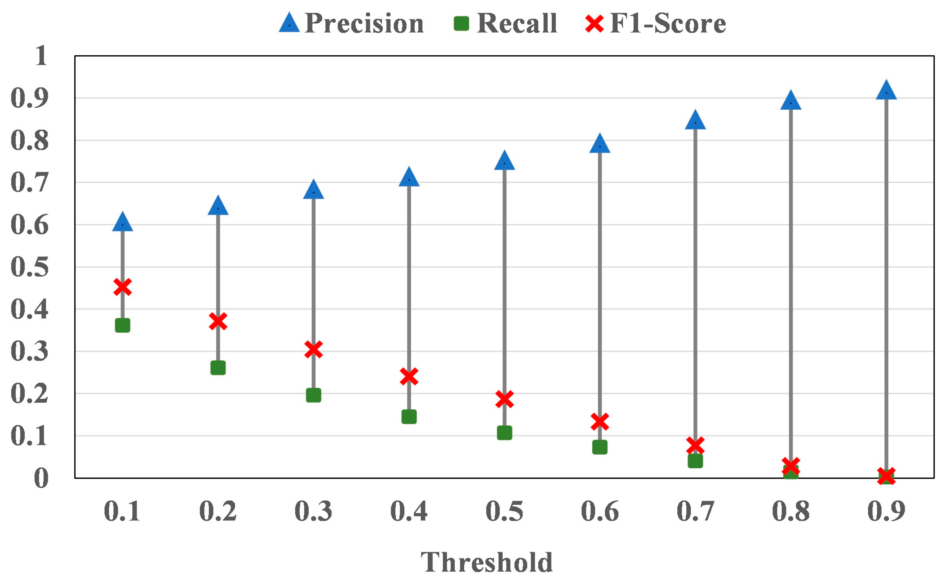
GHSB	2018	10 m	Sentinel	Continent	(Binarized with a threshold of 0.2) the average balanced accuracy of the seven continents is greater than 0.7, and that of Asia is more than 0.875.	Built-up area
CISC	2020	30 m	Landsat	China	No overall accuracy was reported; precision of impervious surface is 94.9% and its recall is 93.7%.	Impervious surface
GL30	2020	30 m	Landsat	Global	The overall accuracy of data in 2020 is 85.72%; no details for specific type.	Land cover
FCS30	2020	30 m	Landsat	Global	The overall accuracy of data in 2020 is 82.5%, and the kappa score is 0.784; the impervious surface in FCS30 was mapped separately, whose overall accuracy is 95.1% and the kappa score is 0.898 [27].	Land cover
WC10	2020	10 m	Sentinel	Global, Continent	The overall accuracy is 74.4 ± 0.1% for global and 80.7 ± 0.1% for Asia; precision for built-up is 67.7 ± 0.9% for global and 69.6 ± 1.4% for Asia; its recall is 67.9 ± 0.8% for global and 69.1 ± 1.4% for Asia.	Land cover
DW	2020	10 m	Sentinel	None	DW was generated by a near real-time land-cover mapping model, which output customized results according to the user-defined temporal and spatial range, so the specific map has no accuracy reported.	Land cover

. The seven products include both thematic maps and land cover products, four have a spatial resolution of 30 m and the other three have a resolution of 10 m. We used 2020 data for five products, namely CISC, GL30, FCS30, WC10 and DW, while the latest versions of both GAIA and GHSB were released in 2018, and, considering their wide recognition, we used the 2018-GAIA and 2018-GHSB as supplementary data and evaluated them together with the 2020 data to explore the feasibility of directly applying these two 2018 datasets to those of 2020. For land cover maps with multiple categories, only the layer associated with impervious surfaces was selected for analysis.

The GHSB is a probabilistic map whose pixel value represents the probability of “human settlement” pixels. A paper verified that the threshold of 0.2 was suitable for Asia to generate a binary classification with a high average balanced accuracy [32]. However, we calculated the precision, recall and F1-Score of the binary outputs derived from GHSB in 2018 on the QTP with thresholds from 0.1 to 0.9 using the validation set, which will be described in detail in Section 2.3.1. The results, summarized in Figure 2, showed that as the binarization threshold grew, the precision increased and the recall and F1-Score decreased. On balance, the threshold of 0.1 gave the highest accuracy for the impervious surface. Thus, the 0.1 was adopted to binarize GHSB for later accuracy assessment rather than the 0.2 recommended.

DW is a near-real-time land cover product generated in near real-time based on user requirements, which uses Sentinel-2 imagery with less than 35% cloud cover by default. We generated the DW land cover data for the QTP in 2020 on the Google Earth Engine platform and used it for later assessment.

2.2.1. Reported Accuracy Comparison

Table 2 collected the accuracy reported by the products producers. GAIA is an impervious surface annual map from 1985 to 2018, which was assessed every five years starting in 1985, and without quality information from the 2018 products. Therefore, Table 2 recorded the results of 2015, which is closest to 2018, as a reference. In addition, due to the nature of DW, which relies on user-defined information and outputs in near real-time, no accuracy description was available for the data we generated.

Of the six products with official accuracy information, only GHSB chose a validation metric inconsistent with the other products, namely balanced accuracy. Balanced accuracy is able to avoid the overestimation of overall accuracy due to unbalanced datasets and is suitable for evaluating the built-up area category whose proportion is much smaller than the natural surface. Moreover, the remaining five products used the common evaluation system, consisting of an overall accuracy/subclass precision/subclass recall. However, the overall accuracy is strongly influenced by the accuracy of the more dominant subcategories. Instead, precision and recall are more convincing for the impervious surface category, which accounts for a much smaller area than the other categories, in order to measure its quality. Nevertheless, only three of these five products (GAIA, CISC and WC10) provided the two indicators of precision and recall in the products, with the results of GAIA displaying two years of temporal errors. In addition, the spatial scales of these three products’ evaluations are only partially consistent, which makes it difficult to compare the quality of different data based on the information supplied.

2.2.2. Mapping of Categories Related to Impervious Surfaces

There are various definitions of the categories related to “impervious surface” in the field of remote sensing, and Zhao et al. [46] systematically summarized the relationship between different concepts, considering that “impervious surface” is a subset of “built-up area”, which is also a subset of “artificial surface.” However, these concepts are not standardized and unified in practice, and the relationship between the categories used in the existing data does not correspond to them. There are cases where the definitions of classes with the same name vary from product to product due to different research contexts and application objectives, so the relationships between the categories related to impervious surfaces of different products need to be re-analyzed based on their detailed definitions.

The names and definitions of the categories related to impervious surfaces for these seven products are shown in

Table 3. Definitions of the impervious surface-related categories extracted from the seven products.

Product Name	Class Name	Definition	Literature
GAIA	Artificial impervious areas	“Artificial impervious areas are mainly man-made structures that are composed of any material that impedes or prevents natural infiltration of water into the soil. They include roofs, paved surfaces, hardened grounds, and major road surfaces mainly found in human settlements.”	Gong et al. [26]
GL30	Artificial Surfaces	“It refers to the surfaces formed by man-built activities. All kinds of habitation in urban and rural areas, industrial and mining area, transportation facilities etc. are included in this category, while interior contiguous green land and water bodies in the construction land use.”	Quote from GL30 official website [51]: http://www.globeland30.org/, accessed on 4 November 2022.
FCS30	Impervious surfaces	“Impervious surfaces are usually covered by anthropogenic materials which prevent water penetrating into the soil and are primarily composed of asphalt, sand and stone, concrete, bricks, glass, etc.”	Zhang et al. [44,45]
CISC	Impervious surfaces	“Impervious surfaces are surfaces covered by various impervious construction materials, such as roofs, roads and squares made of tiles, asphalt, cement concrete, etc.”	Yin [43] Yin et al. [52]
GHSB	Human settlements	“The union of all the satellite data samples that corresponds to a roofed construction above ground which is intended or used for the shelter of humans, animals, things, the production of economic goods or the delivery of services.”	Corbane et al. [32]
WC10	Built-up	“Human made structures; major road and rail networks; large homogenous impervious surfaces including parking structures, office buildings and residential housing; examples: houses, dense villages/towns/cities, paved roads, asphalt.”	Zanaga et al. [33]
DW	Built area	“1. Clusters of human-made structures or individual very large human-made structures; 2. Contained industrial, commercial, and private building, and the associated parking lots; 3. A mixture of residential buildings, streets, lawns, trees, isolated residential structures or buildings surrounded by vegetative land covers; 4. Major road and rail networks outside of the predominant residential areas; 5. Large homogeneous impervious surfaces, including parking structures, large office buildings, and residential housing developments containing clusters of cul-de-sacs.”	Brown et al. [35]

. GAIA, FCS30 and CISC extracted the same objects: artificial impervious surfaces, including all man-made impervious structures, such as buildings and roads. GHSB extracted “human settlements”, which is a subset of “impervious surface”, and compared to “impervious surface”, it does not include roads in its category definition. Although the category name of WC10 is “built-up area”, by definition, it is almost identical to “impervious surface”. The category name of DW is also “built area”, but it has broader extraction targets, including a mixture of vegetation and buildings alongside impervious surfaces. This also applies to GL30, which uses the class name “artificial surfaces”, which includes mining areas in addition to impervious surfaces. The present study summarizes the relationship between the seven product extraction categories, as shown in Figure 3.

However, although definition discrepancies exist, the common objects, impervious surfaces, were still considered to be the majority part of the categories. Thus, from a user’s perspective, we directly mapped the relevant categories as impervious surfaces, which minimized the amount of data pre-processing and reduced the difficulty of applying the products. In this case, the accuracy validation results of GHSB, DW and GL30 data in this paper cannot reflect the factual data accuracy of impervious surface but only offer a reference for data selection when “impervious surface” is the object of study.

2.3. Methodologies for Statistical Accuracy Assessment

2.3.1. Validation Sample Generation

A reliable validation set is the basis for obtaining accurate accuracy assessment results. In order to exactly validate the seven products, we generated a high-accuracy validation set for impervious surfaces on the QTP. Given that the impervious surface accounts for a relatively small proportion of the surface cover, the stratified sampling of positive and negative samples was a more reasonable way to create the validation set [53]. So, the area ratio of permeable and impervious surfaces and their spatial distribution was necessary prior information. The spatial distribution of impervious surfaces in the derived data is highly correlated with the distribution of impervious surfaces in the actual surface [46]. The union of the seven products’ impervious surfaces areas is the maximum distribution of the impervious surfaces jointly determined by these seven datasets. It is also the main distribution area of real, existing impervious surfaces on the QTP. In contrast, the complement of the union represents the main distribution of pervious surfaces.

The validation set takes the form of a grid, as shown in Figure 4, where a primary grid of 30 m × 30 m is composed of 3 × 3 secondary grids of 10 m × 10 m. During the visual interpretation process, the researchers marked only the class of the secondary grids, and the proportion of the categories of the secondary grids was calculated as the class of the primary grids. This sample format allows the cross-resolution accuracy assessments from 10 m to 30 m [54]. The most commonly used sample interpretation base map is Google high-resolution image, but for some areas of the Qinghai–Tibet Plateau, the images in Google Earth are slow to update and imaging time differs significantly from that of the data to be assessed. In order to reduce the assessment errors caused by the temporal discrepancies, the 2020 Chinese GF-1 2 m high-resolution mosaic product was used as the base map for interpretation. Google high-resolution images were only used as supplementary data to provide additional references when interpreting difficult areas. There were three types of categories marked for the secondary grids in the interpretation, namely pervious surface (marked as 0), impervious surface (marked as 1) and mixed grid (marked as 2), and the corresponding interpretation rules were as follows: labeled “0” if no impervious surface objects were in the secondary grid; labeled “1” if impervious surfaces objects were present and their proportion was greater than 50%; labeled “2” if impervious objects were present but their proportion was less than 50%. The primary grid category was then calculated as follows:

$$PC=\frac{W_{notIS}\times n_{notIS}+W_{IS}\times n_{IS}+W_{mixed}\times n_{mixed}}{N_{secondary}}$$

(1)

$$N_{secondary}=n_{notIS}+n_{IS}+n_{mixed}$$

(2)

where $W_{notIS}$, $W_{IS}$ and $W_{mixed}$ are the weights of the three categories of secondary grids contributing to determining the primary grid’s class, with weight values of 0, 1 and 0.5, respectively; $n_{notIS}$, $n_{IS}$ and $n_{mixed}$ denote the number of three categories of secondary grids in a primary grid; and $N_{secondary}$ is the total number of secondary grids in a primary grid, see Equation (2). It is easy to understand that the primary grid is a pervious surface when the PC is 0 and an impervious surface when it is 1. The PC values in the (0, 1) interval indicate different degrees of mixing between pervious and impervious surfaces. For calculation purposes, the class of the primary grid was mapped according to the interpretation rules: the primary grid was considered to be a mixed grid when the PC value belonged to the interval (0, 0.5) and its class was labeled as impervious surface when the PC value belonged to (0.5, 1). The mapping formula is:

$$\mathrm{Label}=\left\{\begin{array}{c}pervious surface if PC=0\\ mixed class if 0<PC<0.5\\ impervious surface if PC\ge 0.5\end{array}\right.$$

(3)

The unqualified samples were removed from the interpretation process. The final validation set consisted of 19,950 primary grids, which could be divided into 179,550 secondary grids.

2.3.2. Method of Accuracy Evaluation

The overall accuracy is poorly measured on an unbalanced sample set. Even though the initial positive and negative samples were stratified, their quantity in the validation set after visual interpretation was not necessarily balanced. In particular, the main focus of this paper was on the accuracy of the impervious surface category in the products. Consequently, the final accuracy validation metrics chosen included the precision, recall and F1-Score of the impervious surface layer. Precision assesses how accurately the product extracted impervious surfaces, while recall quantifies how well the product missed impervious surfaces. Moreover, the F1-Score is the harmonic average of precision and recall, reflecting their comprehensive levels.

In order to investigate the feasibility of using multiple products in combination, in addition to verifying the quality of the products individually, this study also calculated the accuracy metrics of intersection and union sets for different product combinations: ${\mathrm{C}}_4^2$, ${\mathrm{C}}_4^3$ and ${\mathrm{C}}_4^4$ for four 30 m datasets, for a total of 11 intersection and union combinations, and ${\mathrm{C}}_3^2$ and ${\mathrm{C}}_3^3$ for three 10 m resolution products, for a total of four intersection and union combinations.

2.4. Method for Spatial Consistency Analysis

In this paper, consistency analysis was carried out using an impervious surface vote map, which characterizes the spatial frequency distribution of impervious surfaces from different products. The number of votes, namely the pixel value in the vote map, is a composite view of different products on the classification for the same spatial location, directly reflecting the consistency and divergence of each product’s classification results for different geographical locations. The 10 m resolution impervious surface vote map was generated as follows: first, the seven maps were spatially aligned and overlayed; second, the 30 m maps were resampled to 10 m using the nearest neighbor interpolation; then, the frequency of their impervious surface label of the seven maps was counted, with 10 m × 10 m as the minimum unit. Eventually, the frequency distribution of all pixels was the impervious surface vote map, whose values ranged from 0–7 (abbreviated as VC0–VC7), and these values were categorized as the vote class. For example, suppose a pixel was classified as VC3 in the vote map, this means that three of the seven maps classify this pixel as an impervious surface, and the other four classify it as a pervious surface. The same approach, except step two, was adopted to generate the 30 m impervious surface vote map, and a mode sampling method was used instead to downsample the 10 m map into 30 m. Obviously, the higher the proportion of impervious surface objects in a product belonging to the high vote class, the more consistent the product is with others. Conversely, if the extraction result of a product is very different from others, the product’s impervious surface pixels are more likely to belong to the low votes class.

In addition, for a particular pixel, the more votes it receives, the higher probability that its ground truth is impervious surface. To a certain extent, the number of votes reflects the reliability of the pixel category label and correlates with the probability of the pixel being correctly classified. Theoretically, high consistency regions, i.e., high vote class regions, will have higher classification accuracy. In practice, what is the accuracy of different vote regions, the relationship between the number of votes and the accuracy and the number of votes required to obtain high-accuracy impervious surface extraction results? Vote class accuracy (VC Accuracy) is defined as the ratio of the number of pixels correctly classified in vote class i to the total number of pixels in vote class i (see Equation (4)). To explore the above issues, VC Accuracy was used to quantify the impervious surface accuracy of different vote classes. In order to obtain more reasonable results, primary grid samples were used to calculate the VC accuracy of the 30 m vote map and secondary grid samples were adopted for the 10 m map.

$$\mathrm{VC}\mathrm{Accuracy}=\frac{Pixel Number{ }_{True VCi}}{Pixel Number{ }_{Total VCi}}$$

(4)

2.5. Visual Comparison Method

The verification of remote sensing data cannot be separated from visual assessment. This paper selected three distinct regions with different types of impervious surfaces in the QTP: Rikaze, Dujiangyan and Lhasa. These seven products’ impervious surface object characteristics were compared through visual interpretation, such as whether the data boundaries were accurate and whether the extraction structure was complete.

3. Results

3.1. Statistical Accuracy Assessment

The validation results of the seven individual products and intersection and union sets of their different combinations, calculated using the complete validation set, are shown in

Table 4. Validation results of the four 30 m products and their intersection sets and union sets.

Products	Intersection Set			Union Set			IoU	Number of Intersections
	Precision	Recall	F1-Score	Precision	Recall	F1-Score
GAIA	77.31%	9.06%	0.1622	77.31%	9.06%	0.1622	1	401
CISC	87.18%	42.36%	0.5701	87.18%	42.36%	0.5701	1	1662
GL30	66.76%	26.95%	0.3840	66.76%	26.95%	0.3840	1	1381
FCS30	79.55%	19.67%	0.3154	79.55%	19.67%	0.3154	1	846
GAIA + CISC	94.60%	7.69%	0.1422	83.81%	43.73%	0.5747	0.1557	278
GAIA + GL30	86.57%	7.16%	0.1323	65.84%	28.85%	0.4012	0.1888	283
GAIA + FCS30	89.27%	6.81%	0.1266	76.06%	21.92%	0.3404	0.2647	261
CISC + GL30	93.76%	19.76%	0.3264	73.00%	49.55%	0.5903	0.3105	721
CISC + FCS30	95.42%	15.84%	0.2717	81.44%	46.19%	0.5894	0.2928	568
GL30 + FCS30	92.34%	11.98%	0.2122	66.46%	34.64%	0.4554	0.2490	444
GAIA + CISC + GL30	95.59%	6.34%	0.1190	71.75%	50.10%	0.5900	0.0950	227
GAIA+ CISC + FCS30	95.09%	6.23%	0.1169	79.32%	46.97%	0.5900	0.1106	224
GAIA + GL30 + FCS30	92.89%	5.73%	0.1079	65.53%	35.46%	0.4602	0.1140	211
CISC + GL30 + FCS30	96.08%	10.76%	0.1935	70.26%	52.15%	0.5987	0.1508	383
GAIA + CISC + GL30 + FCS30	96.28%	5.29%	0.1003	69.37%	52.56%	0.5980	0.0725	188

and

Table 5. Validation results of the three 10 m products and their intersection sets and union sets.

Products	Intersection Set			Union Set			IoU	Number of Intersections
	Precision	Recall	F1-Score	Precision	Recall	F1-Score
GHSB	60.43%	36.15%	0.4524	60.43%	36.15%	0.4524	1	11345
WC10	73.76%	28.60%	0.4121	73.76%	28.60%	0.4121	1	7354
DW	45.83%	74.32%	0.5670	45.83%	74.32%	0.567	1	30755
GHSB + WC10	84.28%	19.33%	0.3145	60.03%	45.41%	0.5171	0.3032	4351
GHSB + DW	67.66%	34.36%	0.4558	44.46%	76.10%	0.5613	0.2967	9634
WC10 + DW	84.01%	22.35%	0.3531	46.22%	80.56%	0.5874	0.1527	5047
GHSB + WC10 + DW	85.94%	18.65%	0.3065	44.84%	81.66%	0.5790	0.1192	4117

. The results showed that for individual products, the precision was above 75% for 30 m products, except for GL30, which had a precision of 66.76%, with CISC having the highest precision of 87.18%. The recall of all four products was low, with CISC having the top recall of 42.36% and the rest of below 30%, with GAIA being particularly low at only 9.06%. The peak F1-Score obtained by CISC was 0.567, meaning CISC had the best overall performance in precision and recall among the four 30 m products. Among the 10 m products, WC had the highest precision at 73.76%, with GHSB and DW both below 65%. DW had the top recall of 74.32%, followed by GHSB at 36.15% and WC10 at 28.60%. DW obtained the peak F1-Score of 0.5670 of all three products.

Overall, the 30 m products had slightly better precision, while the 10 m maps had slightly better recall. However, there was no significant correlation between the level of accuracy and resolution of the products. The whole recall level of all seven products was low, with all six products below 50%, except for DW, which reached 74.32%, indicating that the omission of impervious surfaces in the QTP region was more severe in each products. Moreover, CISC, with the best quality level among products of both resolutions, was had a similar F1-Score to the DW, indicating that their overall quality level was similar. On the whole, the validation results of each product in the TPQ were lower than their overall accuracy reported officially, which is in line with the common knowledge that the Qinghai–Tibet Plateau is a low-accuracy local area for all products. Furthermore, the misclassification of each product was better than the omission, which was a more serious error.

The results of the two 2018 products, GAIA and GHSB, showed that GAIA had the lowest F1-Score of 0.1622 among the 30 m products, indicating that its overall quality was the worst. The main reason for its poor quality was reflected in its lowest recall, which was most likely caused by the expansion of impervious surfaces in the QTP in the two years between 2018 and 2020. In other words, the most likely and main reason for its poor overall quality was temporal discrepancies. However, its precision was 77.31%, which still demonstrates a strong potential for application. Moreover, the F1-Score of the GHSB was the second lowest of the three 10 m products and not significantly lower than the others, suggesting that utilizing these two 2018 datasets was feasible when conducting the 2020 impervious surface study.

From the intersection and union verification results, intersectional operation improved the precision but decreased the recall. Meanwhile, the considerable loss of recall decreased the F1-Score. On the other hand, the union operation improved the recall but decreased the precision, and the F1-Score increased slightly when the recall rose. The intersection of four 30 m products achieved a precision of 96.28%, but its recall was only 5.29%, with a low F1-Score of 0.1003. The intersection of three 10 m ones achieved a precision of 85.94% and a recall of 18.65%, with an F1-Score of 0.3065. The union of the four products had a precision of 69.37%, with the recall reaching the highest value of 52.56% of the 30 m results, while the union of three 10 m ones’ precision was only 44.84%, but its recall improved to 81.66%. Given the above, the intersection operation was suitable for cases where the data precision was more important than completeness. In contrast, the union operation was appropriate when the data diversity received more attention and a certain amount of noise could be tolerated. Nevertheless, it should be noted that the intersect operation significantly reduced the amount of available data. Specifically, the IoU of both the intersection and union of these combinations was less than 0.32, indicating that the extraction results of impervious surfaces in each product were enormously different; in other words, the impervious surface areas obtained by intersecting and the union were significantly different. Therefore, selecting a specific intersection or union with the best quality for all applications was impossible. The specific categorization and fusion operations of the datasets needed to be decided according to the specific study purpose of the data used. The validation results in Table 4 and Table 5 provided a quantitative reference for future data selection.

Figure 5 compares the evaluation results for individual products using the complete validation set and those calculated using the strict validation set. Compared to the results calculated by categorizing mixed grids as impervious surfaces, the results of the strict validation set showed a slight decrease in precision but a significant increase in recall for all products, such as CISC, GL30 and FCS30. It indicated that the impervious surface missed by each product was mainly mixed pixels with a smaller percentage of impervious surface, which meant all the products’ models were better at detecting pixels with higher percentages of impervious surface.

3.2. Spatial Consistency Analysis

This study analyzed the spatial consistency of the seven products through impervious surface vote maps. Figure 6 shows the ratio of the total pixels number of VC0–VC7 (the vote class in the 10 m vote map had the same ratio as in the 30 m one, so only the 10 m map was used as an example). VC1–VC7 was the maximum impervious surface extent in the QTP voted by these seven products jointly. This maximum extent was only 0.82% of the total study area, which meant that artificial impervious surfaces in the vast QTP were only a tiny subset of the total land cover. For the seven categories VC1–VC7, as the number of votes increased, the area proportion of the corresponding VC class decreased significantly, with VC1 accounting for nearly two thirds and the sum of VC2–VC7 accounting for only one third. The spatial range where the number of votes was greater than or equal to four was considered the high consistency area. The overall percentage of high consistency area was less than 1/6, which was 15.18%. The absolute consistency area, VC1, with votes of all seven products unanimously, was only 2.61%. Hence, the impervious surfaces on the QTP belonging to the high consistency category were few, and the classification results of the seven products were controversial.

Figure 7 shows the source of votes for each VC class in the impervious surface vote map. The proportion of products in the high consistency spatial range was similar for each VC class. In the low consistency area, DW occupied the largest proportion in VC1–VC6, with more than half of the votes in VC1, indicating that the consistency between this product and the others was very low, and a large number of pixels were considered to be impervious surfaces by DW only but pervious surfaces by the others. As can be seen from Table 4 and Table 5, DW had a much higher recall than the other six products, suggesting that other products missed many objects in the pixels that were considered impervious by DW only. GHSB had the second largest percentage in VC1, followed by GL30, and in VC2, the second-largest percentage belonged to CISC, implying that these three maps were also relatively less consistent with the others, with more unique classification opinions.

Nevertheless, all three maps had an F1-Score that ranked highly among the seven products, suggesting that it might be the precision improvement component of the product extraction results that make them different to and inconsistent with the others. This conclusion also indicated that when assessing data consistency in regard to existing products, the reason for poor consistency could either be data anomalies or an improvement in the data quality. Thus, we cannot simply assume that a product with better consistency is of better quality.

Figure 8 shows the results of VC accuracy at 30 m and 10 m calculated using primary and secondary grids. VC accuracy as a whole increased significantly with the number of votes. The VC accuracy of VC1 was poor at 20.76% (10 m) and 39.47% (30 m). In the 30 m vote map, the VC accuracy tended to be stable for VC4–VC7, which were all above 93%, with VC6 obtaining the highest AC accuracy at 96.69%. In the 10 m vote map, the VC accuracy was not over 80% before the votes numbered six. The VC accuracy of VC1–VC6 increased significantly with the increase in votes, and its change slowed down until the votes were greater than six. VC7 was the only category in the 10 m vote map where the VC accuracy exceeds 90% at 92.53% but was still smaller than that of VC7 in the 30 m map. In summary, the validation results of the two resolution vote maps indicated that a reliable impervious surface layer was obtained for both votes greater than or equal to five. The validation accuracy of the same vote class in the 30 m vote map was always greater than that of the 10 m map because the 30 m scale lost more spatial detail compared to 10 m and ignored misclassification at smaller scales, thus improving its accuracy. Figure 9 shows an example where the two misclassifications were ignored when the resolution was downsampled from 10 m to 30 m, resulting in a higher VC accuracy. This also indicated that accuracy assessment results obtained from using the same base map but different spatial units were different, which was consistent with the conclusion from a study [52] that “Estimates of accuracy and area derived from the same map but through the use of different spatial units may be unequal”.

Several vote map localities of typical impervious surfaces on the QTP were selected and are shown in Figure 10. (a) represents Taxkorgan Tajik Autonomous County in the Kashgar prefecture and (b) shows part of the Ngari prefecture; these samples had few impervious surface pixels with votes greater than six, indicating that some products had severe omissions there. The main reason for the above was impervious surfaces’ sparseness and low vegetation coverage in these two regions, which also made it more challenging to extract impervious surfaces accurately. For both the urban areas of (c) Rikaze and (f) Delingha, high consistency areas were mainly present in the densely built-up urban centers. By contrast, (h) Dujiangyan city in Sichuan province, which had a higher vegetation cover, had a more substantial proportion of impervious surface pixels belonging to high consistency areas. Furthermore, high consistency was also displayed among large cities such as (d) Lhasa, (e) Golmud and (g) Xining. Given the above, high-consistency areas were generally concentrated in large urban centers and within clustered buildings. In contrast, urban fringe areas, roads and sparsely built areas commonly received fewer votes and had a smaller high-consistency proportions.

3.3. Visual Comparison

The impervious surfaces layers of different products in three typical areas were visually compared, as displayed in Figure 11, and a detailed comparison is shown in Figure 12, and the layers derived from distinct data showed various characteristics. GAIA had many omissions, probably due to its temporal differences. Likewise, FCS30 neglected many impervious surfaces based on bare ground backgrounds. The impervious surface omissions of GHSB in the Rikaze were severe, which could be caused by the differences in its category definitions. Additionally, GL30 extracted primarily urban and rural outer boundaries without internal details, always with coarse boundaries. WC had the most abundant details, the most accurate portrayal of fine boundaries and a roughly complete extraction of roads, but it was weak when extracting other impervious surfaces types that excluded roads, for instance, in arid western cities, such as the Rikaze, impervious surfaces except roads were missed by WC quite often.

To summarize, the 10 m products generally contained more impervious surface layer detail, but the results became more fragmented as the details were better portrayed. Moreover, the extractions of each product were poorer if the impervious surfaces were on a bare background compared to on a vegetated one.

4. Discussion

4.1. Reasons for Accuracy Underestimation Compared with the Published Accuracy of the Seven Products

The validation accuracy of the products in this paper is lower than the product producers’ reports but does not represent their absolute quality, as we only analyzed them from a user’s perspective on how to use these products; therefore, the adequacy of our methodology and samples to support this conclusion needs to be considered. The reasons for this phenomenon are related to the discrepancies regarding category definition, the temporal differences in the data sources, the scale of data being mapped and the additional challenge of extracting impervious surfaces on the Qinghai–Tibet Plateau:

• Accuracy underestimation due to discrepancies in category definitions: This paper directly adopted the definition of “impervious surface” to rigidly assess products, which was an assessment from the perspective of data users and was oriented towards applying impervious surface products rather than assessing their absolute quality. Thus, discrepancies in category definitions for the three products, GHSB, DW and GL30, whose original categories differed slightly from “impervious surface”, impacted the assessment results;
• Accuracy underestimation due to temporal difference in data sources: GAIA and GHSB were mapped in 2018, in which numerous omissions were found during visual comparison. Some of these omissions might be the new impervious surfaces built after 2018, but this led to an underestimation of recall in the results;
• Accuracy underestimation due to the scale of data being mapped: All products are global products except CISC, which is a product of the region encompassing China. The mapping difficulty of the global products is different from that of the Chinese products. One aspect of this is that it is easier to obtain higher data accuracy when mapping at a smaller spatial scale. Thus, the validation results of the other six products were lower than that of CISC, which only meant that their impervious surface layers’ accuracy in the QTP was lower than that of CISC but was not relevant to the overall quality of the total data or the performance of the data algorithms;
• Accuracy underestimation due to the high heterogeneity of the Qinghai–Tibet Plateau: The high altitude and complex meteorological conditions cause the Qinghai–Tibet Plateau to have fewer available data sources than other regions and make its ground object features much more unique, creating additional difficulties for classification. Thus, the QTP has a generally low local accuracy in all products, and it is reasonable for the local accuracy of the data in QTP to be less than the overall global accuracy.

4.2. Influence of Geo-Registration Errors

Products at different resolutions have a certain level of spatial heterogeneity. Data from different sources also have spatial offset mistakes. The above errors can be directly ignored in low-resolution products but often need to be considered in medium-to-high-resolution images. The validation set used in this paper was geographically registered to Landsat-8 series images, which can be considered to be free of geographical errors with the 30 m datasets, the data source of which was the Landsat series. In addition, the validation grids were geo-aligned with the Sentinel-2 composite images obtained from GEE using GXL (Geoimaging Accelerator) before the validation set was used to assess the 10 m products mapped from the Sentinel-2 series. This paper did not further quantitatively investigate the geographical registration errors between different products. However, according to the accuracy and visual validation results, we found that each product had serious omissions in the QTP, their impervious surface edges were rough and it was extremely difficult to obtain a completely consistent impervious surface boundary from all products. Thus, this paper concluded that the influence of geographical registration errors on the results could be ignored when compared to the classification errors of the products themselves.

5. Conclusions

A wealth of medium-resolution impervious surface products have emerged with a significant increase in available remote sensing data at a medium resolution. From an application perspective, this paper assessed and compared the accuracy of the impervious surface layers of seven products on the Qinghai–Tibet Plateau, namely GAIA, CISC, GL30, FCS30, GHSB, WC10 and DW. The validation set used “impervious surface” as the category definition and was labeled based on the domestic GF-1 satellite with a 2 m resolution. The main conclusions of this paper are as follows:

• The statistical accuracy assessment results showed that CISC and DW had the highest overall quality among the 30 m and 10 m products, with F1-Scores of 0.5701 and 0.5670, respectively. CISC had the best precision at 87.18% and DW had the highest recall at 74.32% of the seven products. All seven products’ local quality in QTP was lower than their global quality, and most products had fewer misclassifications than omissions, which were more serious;
• For the two 2018 supplements, although GAIA had the lowest recall, which might be due to temporal differences, its impervious surface precision was 77.31%, which still had application potential. GHSB’s F1-Score was not the lowest of the 10 m products. Thus, it was feasible to apply the two 2018 products to 2020;
• A union of data combinations is able to improve precision, while an intersection can improve recall. Appropriate data combinations and operations must be chosen according to the study purpose. In addition, the validation results using the strict validation set showed that the impervious surface omissions were mostly mixed pixels with a smaller percentages of impervious surfaces;
• Spatial consistency analysis showed that the maximum impervious surface region on the QTP voted by seven products was only 0.82% of the total area, which was 2,786,800 km², and the high-consistency area (more than four votes) was only 15.18% of this maximum extent;
• The VC accuracy of impervious surface layers with votes greater than three in the 10 m vote map and greater than six in the 30 m map was greater than 80%. In addition, the high-consistency areas were generally concentrated in large urban centers and within clustered buildings, and the low-consistency areas were in urban fringe areas, roads and sparse buildings;
• The visual comparison showed that the 10 m products generally contained more detail, and the extractions were more fragmented when they had more detail. The impervious surface layers with bare backgrounds were of lower quality than those with vegetated backgrounds.

Different data combinations and processing methods fit distinct study purposes, so this paper cannot give a definitive solution of optimal quality. Nevertheless, the validation results above could guide data selection in studies related to impervious surfaces on the QTP: when data accuracy is emphasized more than completeness and data volume, products with high precision and intersection methods can be prioritized. Otherwise, when the diversity of impervious surface samples was the primary demand and certain noises were accepted, products with high recall and a union method might be more suitable. The data volume, precision and recall of the seven products and their intersection and union sets can be found in Section 3 of this paper.

References

- Seto, K.C.; Güneralp, B.; Hutyra, L.R. Global Forecasts of Urban Expansion to 2030 and Direct Impacts on Biodiversity and Carbon Pools. Proc. Natl. Acad. Sci. USA 2012, 109, 16083–16088. [Google Scholar] [CrossRef] [PubMed]
- Arnold, C.L.; Gibbons, C.J. Impervious Surface Coverage: The Emergence of a Key Environmental Indicator. J. Am. Plan. Assoc. 1996, 62, 243–258. [Google Scholar] [CrossRef]
- Slonecker, E.T.; Jennings, D.B.; Garofalo, D. Remote Sensing of Impervious Surfaces: A Review. Remote Sens. Rev. 2001, 20, 227–255. [Google Scholar] [CrossRef]
- Bounoua, L.; Nigro, J.; Zhang, P.; Thome, K.; Lachir, A. Mapping Urbanization in the United States from 2001 to 2011. Appl. Geogr. 2018, 90, 123–133. [Google Scholar] [CrossRef]
- Zhang, J.; Zhang, X.; Tan, X.; Yuan, X. Extraction of Urban Built-up Area Based on Deep Learning and Multi-Sources Data Fusion—The Application of an Emerging Technology in Urban Planning. Land 2022, 11, 1212. [Google Scholar] [CrossRef]
- Angel, S.; Parent, J.; Civco, D.L.; Blei, A.; Potere, D. The Dimensions of Global Urban Expansion: Estimates and Projections for All Countries, 2000–2050. Prog. Plan. 2011, 75, 53–107. [Google Scholar] [CrossRef]
- Yuan, F.; Bauer, M.E. Comparison of Impervious Surface Area and Normalized Difference Vegetation Index as Indicators of Surface Urban Heat Island Effects in Landsat Imagery. Remote Sens. Environ. 2007, 106, 375–386. [Google Scholar] [CrossRef]
- Kafy, A.-A.; Al Rakib, A.; Fattah, M.A.; Rahaman, Z.A.; Sattar, G.S. Others Impact of Vegetation Cover Loss on Surface Temperature and Carbon Emission in a Fastest-Growing City, Cumilla, Bangladesh. Build. Environ. 2022, 208, 108573. [Google Scholar] [CrossRef]
- Boyko, C.T.; Cooper, R.; Davey, C.L.; Wootton, A.B. Informing an Urban Design Process by Way of a Practical Example. Proc. Inst. Civ. Eng.-Urban Des. Plan. 2010, 163, 17–30. [Google Scholar] [CrossRef]
- Yao, T.; Thompson, L.G.; Mosbrugger, V.; Zhang, F.; Ma, Y.; Luo, T.; Xu, B.; Yang, X.; Joswiak, D.R.; Wang, W.; et al. Third Pole Environment (TPE). Environ. Dev. 2012, 3, 52–64. [Google Scholar] [CrossRef]
- Qiu, J. China: The Third Pole. Nature 2008, 454, 393–397. [Google Scholar] [CrossRef] [PubMed]
- Sun, Y.; Liu, S.; Liu, Y.; Dong, Y.; Li, M.; An, Y.; Shi, F.; Beazley, R. Effects of the Interaction among Climate, Terrain and Human Activities on Biodiversity on the Qinghai-Tibet Plateau. Sci. Total Environ. 2021, 794, 148497. [Google Scholar] [CrossRef] [PubMed]
- Yao, T.; Wu, F.; Ding, L.; Sun, J.; Zhu, L.; Piao, S.; Deng, T.; Ni, X.; Zheng, H.; Ouyang, H. Multispherical Interactions and Their Effects on the Tibetan Plateau’s Earth System: A Review of the Recent Researches. Natl. Sci. Rev. 2015, 2, 468–488. [Google Scholar] [CrossRef]
- Tan, K.; Ciais, P.; Piao, S.; Wu, X.; Tang, Y.; Vuichard, N.; Liang, S.; Fang, J. Application of the ORCHIDEE Global Vegetation Model to Evaluate Biomass and Soil Carbon Stocks of Qinghai-Tibetan Grasslands. Glob. Biogeochem. Cycles 2010, 24. [Google Scholar] [CrossRef]
- Kang, S.; Xu, Y.; You, Q.; Flügel, W.-A.; Pepin, N.; Yao, T. Review of Climate and Cryospheric Change in the Tibetan Plateau. Environ. Res. Lett. 2010, 5, 015101. [Google Scholar] [CrossRef]
- Hopping, K.A.; Knapp, A.K.; Dorji, T.; Klein, J.A. Warming and Land Use Change Concurrently Erode Ecosystem Services in Tibet. Glob. Chang. Biol. 2018, 24, 5534–5548. [Google Scholar] [CrossRef]
- Kennedy, C.M.; Oakleaf, J.R.; Theobald, D.M.; Baruch-Mordo, S.; Kiesecker, J. Managing the Middle: A Shift in Conservation Priorities Based on the Global Human Modification Gradient. Glob. Chang. Biol. 2019, 25, 811–826. [Google Scholar] [CrossRef]
- Mu, H.; Li, X.; Wen, Y.; Huang, J.; Du, P.; Su, W.; Miao, S.; Geng, M. A Global Record of Annual Terrestrial Human Footprint Dataset from 2000 to 2018. Sci. Data 2022, 9, 176. [Google Scholar] [CrossRef]
- Liu, T.; Liu, H.; Qi, Y. Construction Land Expansion and Cultivated Land Protection in Urbanizing China: Insights from National Land Surveys, 1996–2006. Habitat Int. 2015, 46, 13–22. [Google Scholar] [CrossRef]
- He, G.; Zhang, Z.; Jiao, W.; Long, T.; Peng, Y.; Wang, G.; Yin, R.; Wang, W.; Zhang, X.; Liu, H.; et al. Generation of Ready to Use (RTU) Products over China Based on Landsat Series Data. Big Earth Data 2018, 2, 56–64. [Google Scholar] [CrossRef]
- He, G.; Wang, L.; Ma, Y.; Zhang, Z.; Wang, G.; Peng, Y.; Long, T.; Zhang, X. Processing of Earth Observation Big Data: Challenges and Countermeasures. Chin. Sci. Bull. 2015, 60, 470–478. [Google Scholar]
- He, G.; Wang, G.; Long, T.; Peng, Y.; Jiang, W.; Yin, R.; Jiao, W.; Zhang, Z. Opening and Sharing of Big Earth Observation Data: Challenges and Countermeasures. Bull. Chin. Acad. Sci. Chin. Version 2018, 33, 783–790. [Google Scholar]
- He, G.; Jiao, W.; Zhang, Z.; Long, T.; Wang, G.; Peng, Y.; Yin, R. Remote Sensing Data Based Ready To Use (RTU) Products. China Sci. Data 2020, 5, 6–13. [Google Scholar]
- Weng, Q. Remote Sensing of Impervious Surfaces in the Urban Areas: Requirements, Methods, and Trends. Remote Sens. Environ. 2012, 117, 34–49. [Google Scholar] [CrossRef]
- Fu, S.; Zhang, X.; Kuang, W.; Guo, C. Characteristics of Changes in Urban Land Use and Efficiency Evaluation in the Qinghai–Tibet Plateau from 1990 to 2020. Land 2022, 11, 757. [Google Scholar] [CrossRef]
- Gong, P.; Li, X.; Wang, J.; Bai, Y.; Cheng, B.; Hu, T.; Liu, X.; Xu, B.; Yang, J.; Zhang, W.; et al. Annual Maps of Global Artificial Impervious Area (GAIA) between 1985 and 2018. Remote Sens. Environ. 2020, 236, 111510. [Google Scholar] [CrossRef]
- Zhang, X.; Liu, L.; Zhao, T.; Gao, Y.; Chen, X.; Mi, J. GISD30: Global 30 m Impervious-Surface Dynamic Dataset from 1985 to 2020 Using Time-Series Landsat Imagery on the Google Earth Engine Platform. Earth Syst. Sci. Data 2022, 14, 1831–1856. [Google Scholar] [CrossRef]
- Wang, P.; Huang, C.; Tilton, J.C.; Tan, B.; de Colstoun, E.C.B. HOTEX: An Approach for Global Mapping of Human Built-up and Settlement Extent. In Proceedings of the 2017 IEEE International Geoscience and Remote Sensing Symposium (IGARSS), Fort Worth, TX, USA, 23–28 July 2017; 2017; pp. 1562–1565. [Google Scholar]
- Liu, X.; Hu, G.; Chen, Y.; Li, X.; Xu, X.; Li, S.; Pei, F.; Wang, S. High-Resolution Multi-Temporal Mapping of Global Urban Land Using Landsat Images Based on the Google Earth Engine Platform. Remote Sens. Environ. 2018, 209, 227–239. [Google Scholar] [CrossRef]
- Gong, P.; Wang, J.; Yu, L.; Zhao, Y.; Zhao, Y.; Liang, L.; Niu, Z.; Huang, X.; Fu, H.; Liu, S.; et al. Finer Resolution Observation and Monitoring of Global Land Cover: First Mapping Results with Landsat TM and ETM+ Data. Int. J. Remote Sens. 2013, 34, 2607–2654. [Google Scholar] [CrossRef]
- Chen, J.; Chen, J.; Liao, A.; Cao, X.; Chen, L.; Chen, X.; He, C.; Han, G.; Peng, S.; Lu, M.; et al. Global Land Cover Mapping at 30m Resolution: A POK-Based Operational Approach. ISPRS J. Photogramm. Remote Sens. 2015, 103, 7–27. [Google Scholar] [CrossRef]
- Corbane, C.; Syrris, V.; Sabo, F.; Politis, P.; Melchiorri, M.; Pesaresi, M.; Soille, P.; Kemper, T. Convolutional Neural Networks for Global Human Settlements Mapping from Sentinel-2 Satellite Imagery. Neural Comput. Appl. 2021, 33, 6697–6720. [Google Scholar] [CrossRef]
- Zanaga, D.; Van De Kerchove, R.; De Keersmaecker, W.; Souverijns, N.; Brockmann, C.; Quast, R.; Wevers, J.; Grosu, A.; Paccini, A.; Vergnaud, S.; et al. ESA WorldCover 10 m 2020 V100 2021. Available online: https://0-doi-org.brum.beds.ac.uk/10.5281/zenodo.5571936 (accessed on 7 March 2023).
- Chen, B.; Xu, B.; Zhu, Z.; Yuan, C.; Suen, H.P.; Guo, J.; Xu, N.; Li, W.; Zhao, Y.; Yang, J.; et al. Stable Classification with Limited Sample: Transferring a 30-m Resolution Sample Set Collected in 2015 to Mapping 10-m Resolution Global Land Cover in 2017. Sci. Bull. 2019, 64, 370–373. [Google Scholar]
- Brown, C.F.; Brumby, S.P.; Guzder-Williams, B.; Birch, T.; Hyde, S.B.; Mazzariello, J.; Czerwinski, W.; Pasquarella, V.J.; Haertel, R.; Ilyushchenko, S.; et al. Dynamic World, Near Real-Time Global 10 m Land Use Land Cover Mapping. Sci. Data 2022, 9, 251. [Google Scholar] [CrossRef]
- Foody, G.M. Status of Land Cover Classification Accuracy Assessment. Remote Sens. Environ. 2002, 80, 185–201. [Google Scholar] [CrossRef]
- Stehman, S.V.; Foody, G.M. Key Issues in Rigorous Accuracy Assessment of Land Cover Products. Remote Sens. Environ. 2019, 231, 111199. [Google Scholar] [CrossRef]
- Xing, H.; Meng, Y.; Hou, D.; Cao, F.; Xu, H. Exploring Point-of-Interest Data from Social Media for Artificial Surface Validation with Decision Trees. Int. J. Remote Sens. 2017, 38, 6945–6969. [Google Scholar] [CrossRef]
- Wickham, J.; Stehman, S.V.; Sorenson, D.G.; Gass, L.; Dewitz, J.A. Thematic Accuracy Assessment of the NLCD 2016 Land Cover for the Conterminous United States. Remote Sens. Environ. 2021, 257, 112357. [Google Scholar] [CrossRef]
- Wang, J.; Yang, X.; Wang, Z.; Cheng, H.; Kang, J.; Tang, H.; Li, Y.; Bian, Z.; Bai, Z. Consistency Analysis and Accuracy Assessment of Three Global Ten-Meter Land Cover Products in Rocky Desertification Region—A Case Study of Southwest China. ISPRS Int. J. Geo-Inf. 2022, 11, 202. [Google Scholar] [CrossRef]
- Gao, Y.; Liu, L.; Zhang, X.; Chen, X.; Mi, J.; Xie, S. Consistency Analysis and Accuracy Assessment of Three Global 30-m Land-Cover Products over the European Union Using the LUCAS Dataset. Remote Sens. 2020, 12, 3479. [Google Scholar] [CrossRef]
- Chen, J.; Yan, F.; Lu, Q. Spatiotemporal Variation of Vegetation on the Qinghai–Tibet Plateau and the Influence of Climatic Factors and Human Activities on Vegetation Trend (2000–2019). Remote Sens. 2020, 12, 3150. [Google Scholar] [CrossRef]
- Yin, R. Research on Impervious Surface Coverage and Change Information Mining Methods in Large-Scale and Long Time Series. Ph.D. Thesis, Aerospace Information Research Institute, Chinese Academy of Sciences, Beijing, China, 2022. [Google Scholar]
- Zhang, X.; Liu, L.; Wu, C.; Chen, X.; Gao, Y.; Xie, S.; Zhang, B. Development of a Global 30 m Impervious Surface Map Using Multisource and Multitemporal Remote Sensing Datasets with the Google Earth Engine Platform. Earth Syst. Sci. Data 2020, 12, 1625–1648. [Google Scholar] [CrossRef]
- Zhang, X.; Liu, L.; Chen, X.; Gao, Y.; Xie, S.; Mi, J. GLC_FCS30: Global Land-Cover Product with Fine Classification System at 30 m Using Time-Series Landsat Imagery. Earth Syst. Sci. Data 2021, 13, 2753–2776. [Google Scholar] [CrossRef]
- Zhao, Y.; Zhu, Z. ASI: An Artificial Surface Index for Landsat 8 Imagery. Int. J. Appl. Earth Obs. Geoinf. 2022, 107, 102703. [Google Scholar] [CrossRef]
- Yang, F.; Wang, Z.; Yang, X.; Liu, Y.; Liu, B.; Wang, J.; Kang, J. Using Multi-Sensor Satellite Images and Auxiliary Data in Updating and Assessing the Accuracies of Urban Land Products in Different Landscape Patterns. Remote Sens. 2019, 11, 2664. [Google Scholar] [CrossRef]
- Zhang, W.; Wang, J.; Lin, H.; Cong, M.; Wan, Y.; Zhang, J. Fusing Multiple Land Cover Products Based on Locally Estimated Map-Reference Cover Type Transition Probabilities. Remote Sens. 2023, 15, 481. [Google Scholar] [CrossRef]
- Huang, X.; Song, Y.; Yang, J.; Wang, W.; Ren, H.; Dong, M.; Feng, Y.; Yin, H.; Li, J. Toward Accurate Mapping of 30-m Time-Series Global Impervious Surface Area (GISA). Int. J. Appl. Earth Obs. Geoinf. 2022, 109, 102787. [Google Scholar] [CrossRef]
- Venter, Z.S.; Barton, D.N.; Chakraborty, T.; Simensen, T.; Singh, G. Global 10 m Land Use Land Cover Datasets: A Comparison of Dynamic World, World Cover and Esri Land Cover. Remote Sens. 2022, 14, 4101. [Google Scholar] [CrossRef]
- Global Land Cover—Product Introduction. Available online: http://www.globeland30.org/Page/EN_sysFrame/dataIntroduce.html?columnID=81&head=product¶=product&type=data (accessed on 25 February 2023).
- Yin, R.; He, G.; Wang, G.; Long, T.; Li, H.; Zhou, D.; Gong, C. Automatic Framework of Mapping Impervious Surface Growth With Long-Term Landsat Imagery Based on Temporal Deep Learning Model. IEEE Geosci. Remote Sens. Lett. 2022, 19, 1–5. [Google Scholar] [CrossRef]
- Olofsson, P.; Foody, G.M.; Herold, M.; Stehman, S.V.; Woodcock, C.E.; Wulder, M.A. Good Practices for Estimating Area and Assessing Accuracy of Land Change. Remote Sens. Environ. 2014, 148, 42–57. [Google Scholar] [CrossRef]
- See, L.; Georgieva, I.; Duerauer, M.; Kemper, T.; Corbane, C.; Maffenini, L.; Gallego, J.; Pesaresi, M.; Sirbu, F.; Ahmed, R.; et al. A Crowdsourced Global Data Set for Validating Built-up Surface Layers. Sci. Data 2022, 9, 13. [Google Scholar] [CrossRef]