
Deep Learning for Integrated Speckle Reduction and Super-Resolution in Multi-Temporal SAR
1
School of Automation and Electronic Information, Xiangtan University, Xiangtan 411105, China
2
School of Mathematics and Computational Science, Xiangtan University, Xiangtan 411105, China
3
National Center for Applied Mathematics in Hunan Laboratory, Xiangtan 411105, China
*
Author to whom correspondence should be addressed.
†
These authors contributed equally to this work.
Remote Sens. 2024, 16(1), 18; https://0-doi-org.brum.beds.ac.uk/10.3390/rs16010018
Submission received: 15 September 2023
/
Revised: 8 December 2023
/
Accepted: 13 December 2023
/
Published: 20 December 2023
(This article belongs to the Special Issue Advance in SAR Image Despeckling)
Abstract
:In the domain of synthetic aperture radar (SAR) image processing, a prevalent issue persists wherein research predominantly focuses on single-task learning, often neglecting the concurrent impact of speckle noise and low resolution on SAR images. Currently, there are two main processing strategies. The first strategy involves conducting speckle reduction and super-resolution processing step by step. The second strategy involves performing speckle reduction as an auxiliary step, with a focus on enhancing the primary task of super-resolution processing. However, both of these strategies exhibit clear deficiencies. Nevertheless, both tasks jointly focus on two key aspects, enhancing SAR quality and restoring details. The fusion of these tasks can effectively leverage their task correlation, leading to a significant improvement in processing effectiveness. Additionally, multi-temporal SAR images covering imaging information from different time periods exhibit high correlation, providing deep learning models with a more diverse feature expression space, greatly enhancing the model’s ability to address complex issues. Therefore, this study proposes a deep learning network for integrated speckle reduction and super-resolution in multi-temporal SAR (ISSMSAR). The network aims to reduce speckle in multi-temporal SAR while significantly improving the image resolution. Specifically, it consists of two subnetworks, each taking the SAR image at time 1 and the SAR image at time 2 as inputs. Each subnetwork includes a primary feature extraction block (PFE), a high-level feature extraction block (HFE), a multi-temporal feature fusion block (FFB), and an image reconstruction block (REC). Following experiments on diverse data sources, the results demonstrate that ISSMSAR surpasses speckle reduction and super-resolution methods based on a single task in terms of both subjective perception and objective evaluation metrics regarding the quality of image restoration.
1. Introduction
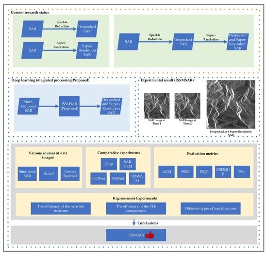
SAR is a remote sensing technology that generates high-quality images by processing pulse signals. The working wavelength of SAR ranges from 1 cm to 1 m, whereas camera sensors use wavelengths closer to visible light or 1 micron [1]. Therefore, SAR exhibits excellent penetration capability and can acquire high-quality remote sensing data in adverse weather conditions such as clouds, haze, rain, or snow, making it an all-weather remote sensing technology [2,3,4,5,6]. However, in the process of SAR imaging, the generation of speckle noise is inevitable [7], which significantly affects the quality and resolution of SAR images [8]. To overcome this issue, there are currently two main strategies:
The first strategy adopts a two-stage processing approach, performing speckle reduction and super-resolution processing step by step. This is due to the fact that, in the presence of speckle noise, directly applying super-resolution processing to SAR images may amplify the speckle noise, thereby making it very prominent in the resulting image. Therefore, speckle reduction is applied to the SAR image first to mitigate the impact of speckle noise. Subsequently, super-resolution processing is employed to enhance spatial resolution while maintaining image clarity [9].
The essence of the step-by-step strategy lies in explicitly separating the speckle reduction and super-resolution processes, which means treating speckle reduction and super-resolution processing as two independent processes. By employing common speckle reduction and super-resolution methods, this processing procedure is implemented in a step-by-step manner. In the speckle reduction process of SAR images, there are primarily two categories of methods: traditional speckle reduction algorithms and deep learning algorithms [10]. Traditional speckle reduction algorithms include classical methods such as Frost [11], non-local means (NLMs) [12], and ratio image speckle reduction [13], etc. In recent years, with the rapid development of deep learning, it has demonstrated outstanding performance in computer vision tasks. Researchers have proposed a series of efficient deep learning algorithms for speckle reduction. These include FFDNet [14], SAR2SAR [15], AGSDNet [16], etc. In terms of super-resolution reconstruction in SAR images, there are also two categories of methods: traditional super-resolution algorithms and deep learning algorithms [17]. Traditional super-resolution methods include interpolation methods [18] and ScSR [19], etc. Commonly used interpolation methods include nearest neighbor interpolation and bilinear interpolation [20]. Due to their low computational complexity and high speed, they have become one of the most popular methods for rendering super-resolution images [21]. However, it is worth mentioning that most deep learning-based super-resolution methods for SAR images often directly transfer processing strategies from optical images without fully considering the special properties of SAR imaging, which may to some extent affect the accuracy and stability of the reconstruction results [22].
However, when conducting a simple step-by-step strategy, which involves speckle reduction followed by super-resolution, the results often turn out to be unsatisfactory. This is because the speckle reduction stage alone may lead to the loss of some high-frequency details, making it impossible to fully recover them in the subsequent super-resolution process. Additionally, the speckle reduction stage inevitably introduces some erroneous restoration, which may be amplified in the subsequent super-resolution process, leading to a decrease in the final result’s quality [23]. Zhao et al. pointed out that due to the significant amplitude and phase fluctuations caused by speckle noise, even with the use of state-of-the-art spatial speckle reduction methods (such as SAR-BM3D or SAR-NLM), the image structure may still be disrupted [13], and some noticeable speckle fluctuations may be retained after speckle reduction. Furthermore, in Zhan et al.’s work [24], the preprocessing of TERRA-SAR images (including speckle reduction) resulted in a loss of image structure. In subsequent super-resolution processing, the phenomenon of structural loss can be observed to be significantly amplified. This emphasizes the inherent limitations in the step-by-step strategy. In summary, the straightforward step-by-step strategy of speckle reduction followed by super-resolution exhibits significant drawbacks when processing SAR images.
The second strategy involves performing speckle reduction as an auxiliary step, with a focus on enhancing the primary task of super-resolution processing. This approach represents a relatively comprehensive strategy for SAR image processing. In this regard, several studies have proposed a series of methods. Among them, Wu et al. introduced an improved NLM method combined with a back-propagation neural network [25]. Through this approach, the enhanced NLM not only significantly improves low-resolution images to high-resolution levels but also effectively reduces speckle in SAR images. Kanakaraj et al. proposed a new method for SAR image super-resolution using the importance sampling unscented Kalman filter, which has the capability to handle multiplicative noise [26]. On the other hand, Karimi et al. introduced a novel convex variational optimization model focused on the single-image super-resolution reconstruction of SAR images with speckle noise [27]. This model utilizes Total Variation (TV) regularization to achieve edge preservation and speckle reduction. Additionally, Luo et al. introduced the combination of cubature Kalman filter and low-rank approximation, constructing a nonlinear low-rank optimization model [28]. Finally, Gu et al. presented the Noise-Free Generative Adversarial Network (NF-GAN), which utilizes a deep generative adversarial network to reconstruct pseudo-high-resolution SAR images [29]. However, it is worth emphasizing that these methods have certain limitations in speckle reduction. For detailed information, refer to Table 1. Overall, they may exhibit two potential issues: on one hand, they may show a tendency towards excessive smoothing, meaning that image details are excessively blurred during the speckle reduction process, weakening specific image features; on the other hand, the speckle reduction effect may not be sufficiently thorough, leaving traces of speckle noise, which affects the clarity and level of detail in the image. This strategy primarily focuses on prioritizing super-resolution processing, while speckle reduction is relatively secondary. This also suggests that researchers need to seek more comprehensive and refined processing strategies in their future work, especially specialized approaches for speckle noise, in order to achieve the comprehensive optimization of SAR images.
In order to overcome the aforementioned issues, it is imperative to adopt a novel strategy that involves deep exploration of the underlying correlations between speckle reduction and super-resolution in SAR images. This approach aims to achieve more effective speckle reduction and super-resolution processing for SAR images. Recognizing that both speckle reduction and super-resolution processing require high-quality image reconstruction, they exhibit significant correlation. This is because they primarily focus on processing the high-frequency components while simultaneously preserving other crucial information [30]. Additionally, multi-temporal SAR images are typically acquired by the same satellite at different times for the same target scene, containing rich spatiotemporal information. Compared to single-temporal SAR images, they provide a more abundant source of information [31]. Utilizing multi-temporal SAR images as input for the network enables the network to comprehensively understand the characteristics of objects, thereby better preserving spatial resolution [13] and providing favorable conditions for high-quality image reconstruction.
Given that these two tasks mutually reinforce each other, it is essential to develop a novel approach that integrates them into a unified deep learning model. Therefore, this paper proposes ISSMSAR. The objective of this network framework is to process two input multi-temporal SAR images. Through a series of processing modules, including PFE, HFE, FFB, and REC, the aim is to obtain the final high-quality SAR image.
The main contributions of this paper include the following:
- This study proposes, for the first time, an integrated network framework utilizing deep learning for speckle reduction and super-resolution reconstruction of multi-temporal SAR images.
- Based on the characteristics of SAR images, PFE is designed, incorporating three key innovative elements: parallel multi-scale convolution feature extraction, multi-resolution training strategy, and high-frequency feature enhancement learning. These innovations enable the network to more accurately adapt to the complex features of SAR images.
- In the HFE, a clever fusion of techniques including deconvolution, deformable convolution, and skip connections is employed to precisely extract more complex and abstract features from SAR images.
- Drawing inspiration from the traditional SAR algorithm, the network introduces the ratio-L1 loss as the optimization objective. Additionally, a hierarchical loss constraint mechanism is introduced to ensure the effectiveness of each critical module, thereby guaranteeing the robustness and reliability of the overall network performance.
- Approaching from the perspective of multi-task learning, a dataset named “Multi-Task SAR Dataset” is proposed to provide solid support and foundation for the fusion learning task of speckle reduction and super-resolution of multi-temporal SAR images.
The structure of this paper is as follows: The second section will provide a detailed exposition of the network architecture of ISSMSAR and the ratio-L1 loss function. The third section will elucidate the process of creating the Multi-Task SAR Dataset, presenting concrete experiments and corresponding in-depth analyses. The fourth section will conclude this study.
2. Methodology
In this section, a statistical analysis of SAR images is initially conducted. Following that, a detailed exposition of the ISSMSAR architecture proposed in this study is provided. Finally, the ratio-L1 loss function and the hierarchical loss constraint mechanism proposed in this study are discussed in detail.
2.1. Signal Statistical Description
In SAR image processing, speckle noise belongs to a special form of noise categorized as multiplicative noise. The characteristic of multiplicative noise is that its amplitude is proportional to the amplitude of the signal, resulting in the noise amplitude varying proportionally with the strength of the signal. This noise model can be expressed as follows:
In this equation, represents the observed SAR image containing speckle, denotes the clean image unaffected by speckle noise, and represents the speckle noise. The statistical characteristics of speckle noise are widely acknowledged to follow a gamma distribution. The probability density function of the gamma distribution can be expressed by the following equation:
In this formula, represents the random variable, denotes the shape parameter, and represents the gamma function.
2.2. Network Architecture
The construction of the ISSMSAR is rooted in the multi-task learning of multi-temporal SAR images, aiming to thoroughly exploit the feature information among these images for the integrated speckle reduction and super-resolution processing of SAR images. The network architecture, as illustrated in Figure 1, encompasses two subnetworks and primarily comprises seven crucial components: multi-temporal image inputs, primary feature extraction block, high-level feature extraction block, multi-temporal feature fusion block, image reconstruction block, post-processed image output, and the loss function. The network takes as input SAR images at time 1 and time 2. After processing through the network, it ultimately outputs the processed SAR image, as expressed in Equation (3).
Here, represents the entire process carried out by the ISSMSAR, encompassing all processing steps from input to output. and denote the two input multi-temporal SAR images, serving as the starting point of the network’s processing. represents the SAR image result obtained after the entire operation of the ISSMSAR.
2.2.1. Primary Feature Extraction Block
The primary feature extraction block, as shown in Figure 2, aims to capture fundamental feature information shared between the tasks of speckle reduction and super-resolution from the input multi-temporal SAR images. Specifically, this module takes two multi-temporal SAR images labeled as and as input. Subsequently, after processing through the PFE, corresponding primary features and are extracted, calculated according to Equations (4) and (5), respectively.
Here, represents the operation of the PFE. Through the processing of this module, fundamental features are extracted from each input image, providing crucial foundational information for subsequent processing steps.
Figure 2.
Primary feature extraction block.

In this module, a series of innovative solutions has been introduced, including parallel multi-scale convolutional feature extraction, multi-resolution training strategy, and high-frequency feature enhancement learning, to address the challenge of speckle noise in SAR images.
Due to the presence of speckle noise, SAR images exhibit irregular patterns of brightness and darkness, resulting in less distinct boundaries and features between objects in the image. In some cases, they might even be obscured, potentially leading to misinterpretations during the learning process. To tackle this issue, this study proposes an optimization strategy: employing parallel multi-scale convolutions for fundamental feature extraction. This approach significantly enhances the network’s feature extraction capability, providing a more comprehensive feature representation.
Three parallel multi-scale convolutional structures were designed utilizing different kernel sizes, including 3 × 3, 5 × 5, and 7 × 7. Specifically, the 3 × 3 convolutional kernel has a smaller receptive field, focusing on local details in the image, which helps the network learn finer feature information. The 5 × 5 convolutional kernel is used to capture medium-scale structural and textural features, with a receptive field falling between 3 × 3 and 7 × 7, making it better suited for capturing medium-scale features. The 7 × 7 convolutional kernel is suitable for capturing larger-scale structural information. Compared to the 3 × 3 and 5 × 5 convolutional kernels, the larger receptive field covers a wider local area, thus acquiring more complex and abstract feature information. This strategy significantly reduces the impact of speckle noise on object information in SAR images, effectively enhancing feature extraction capability. This optimization strategy takes into full consideration the unique noise characteristics of SAR images, providing robust support for the feature extraction stage of the network, thereby establishing a solid foundation for subsequent processing steps.
When replicating other networks, a common challenge is the potential insufficiency of the network’s generalization ability. This is particularly pronounced when there are disparities in the data sources between the test set and the training set, resulting in differing resolutions of SAR images. Consequently, the performance of test results is often below expectations. To address this issue, this study introduces a multi-resolution training strategy, aimed at enabling the model to learn features from input images of varying resolutions during the training phase, thus enhancing its generalization ability.
Specifically, this module downsampled the input SAR images using a downsampling factor of 2. The original SAR image had a size of 512 × 512. After downsampling, the image resolution was reduced to 256 × 256. Subsequently, multi-scale convolutional feature extraction was conducted on this reduced-resolution image. To ensure that the size of the extracted features remained consistent with the results of other parallel multi-scale convolutions, this study performed an upsampling operation on the feature maps. This process restored the feature maps of the low-resolution image to the same size as the other scales, maintaining consistency in parallel processing. The introduction of this strategy in the training phase provided the model with the ability to learn features from input images of different resolutions, thereby enhancing its generalization capability on test data with resolution disparities.
In SAR images, speckle noise and edge details are primarily distributed in the high-frequency components. Therefore, speckle reduction and super-resolution processing primarily target high-frequency information. To enhance the network’s learning of high-frequency features, high-frequency feature enhancement learning is introduced, as illustrated in Figure 3. This module aims to extract high-frequency information from the original SAR image and reintroduce these high-frequency features into the network for learning. In this way, the network can better understand the characteristics of speckle noise. Additionally, this module is capable of capturing edges and details in the image, thereby enhancing the preservation of detailed information in image processing.
The specific operations are as follows: first, discrete wavelet transform (DWT) is used to decompose the SAR image into high-frequency and low-frequency components. Next, the low-frequency component is replaced with a zero tensor, and inverse discrete wavelet transform (IDWT) is performed to extract the high-frequency information from the SAR image. Subsequently, multi-scale convolutional feature extraction is applied to the extracted high-frequency information.
Finally, a feature concatenation operation is performed on the parallel multi-scale convolutional results to form a multi-scale feature representation. Subsequently, the ReLU activation function is applied, and an ECA attention mechanism [32] is introduced to obtain the final output of the PFE.
2.2.2. High-Level Feature Extraction Block
The high-level feature extraction block is designed to extract more abstract features from primary features, as illustrated in Figure 4. This block consists of multiple sets of deconvolutions and deformable convolutions, incorporating a mechanism for skip connections.
The deconvolution operation has the capability to upsample low-resolution feature maps to higher resolution, allowing for the recovery of more detailed structural information. Moreover, in contrast to fixed-shape convolutional kernels, deformable convolutions can more effectively capture minute details and morphological changes in the image. Moreover, the introduction of deformable convolutions enhances the flexibility of feature extraction, enabling the kernel to adapt its shape to accommodate detailed features in different regions.
The alternating use of deconvolution and deformable convolution strategies enhances the network’s contextual awareness, aiding in the global understanding of the image’s overall structure. The incorporation of skip connections between convolution and deconvolution operations effectively transfers primary features to higher levels, enabling feature information to flow between different levels. This provides the network with richer feature representation and learning capabilities.
Therefore, after the operation of the HFE, the primary features and are mapped according to their corresponding high-level features and . This mapping relationship can be expressed by the following two equations:
Here, represents the specific operation of the HFE. This step is a crucial component of the network, as high-level feature extraction allows the network to better comprehend and abstract the characteristics present in SAR images.
To reconstruct the super-resolution image, the reconstruction block is used to map and to a high-resolution image. The REC consists of a deconvolution layer followed by a convolution layer. Taking into account the skip connection, the final super-resolution image after SRB can be obtained by adding the bilinear upsampled image to the reconstructed residual image:
where represents the operation of bilinear upsampling, and represents the operation of the image reconstruction block.
2.2.3. Multi-Temporal Feature Fusion block
In the multi-temporal feature fusion block, three interconnected inter-channel feature synergy (IFS) modules are employed, as illustrated in Figure 5. The IFS module is inspired by the CFB module introduced in [33]. It lies in the incorporation of convolutional layers with parametric rectified linear units (PReLUs), as well as 1 × 1 convolutions and deconvolutional layers with PReLUs. These components are closely coupled through multiple intricate skip connections. Each IFS module takes three inputs: the primary features extracted by PFE, the output of the previous module in the same sub-path, and the output of the previous module in the other sub-path.
Here, , , and represent the operations of IFS1, IFS2, and IFS3, respectively. , , and represent the outputs of IFS1, IFS2, and IFS3, respectively.
Here, , and represent the operations of IFS1′, IFS2′, and IFS3′, respectively. , , and represent the outputs of IFS1′, IFS2′, and IFS3′, respectively.
After each IFS, the reconstructed image can be obtained as follows:
2.2.4. Fusion Image Output
Since the network structure consists of two subnetworks, the outputs of IFS3 and IFS3’ are denoted as and , respectively. In order to comprehensively utilize the information extracted by both subnetworks to obtain a more accurate final result, and are combined through a weighted summation to obtain the ultimate output of the entire network, denoted as , as specifically expressed in Equation (22).
2.3. Cost Function
2.3.1. Ratio-L1 Loss
Based on the correlation characteristics of SAR, this study proposes the ratio-L1 loss. The algorithm combines the ratio loss and L1 loss, constructing a comprehensive loss function that considers both global and detail levels. This loss function effectively guides the training of the network.
Inspired by [13], we introduced a ratio operation between the pixel average value of the processed SAR image and the pixel average value of the clear super-resolution SAR image in the loss function, as shown in Equation (23). This ratio loss can guide the speckle reduction process on a global scale, contributing to speckle reduction in the overall image. Moreover, the proposed ratio loss considers the entire image, unlike methods that perform ratio at the pixel level. This helps to reduce the risk of overfitting.
where represents the clean high-resolution SAR image, represents the SAR image output by the network, xi represents the -th pixel value in , and represents the -th pixel value in .
Due to the limitation of the ratio loss in handling fine details, details might be overlooked. To achieve a balanced performance in the loss function, we introduced the L1 loss as a complement. The L1 loss is a commonly used method for measuring the error between predicted and true values. In this algorithm, we applied L1 loss to calculate the average absolute difference between each pixel in the clean high-resolution SAR image and the network output SAR image, as shown in Equation (24). This supplementary measure aims to further enhance the comprehensive performance of the loss function.
where represents the clean high-resolution SAR image, represents the SAR image output by the network, represents the -th pixel value in , and represents the -th pixel value in .
2.3.2. Hierarchical Loss Constraint Mechanism
Given the complexity of ISSMSAR, a hierarchical loss constraint mechanism is introduced to guarantee the overall training performance of key modules in the network, as shown in Equations (25)–(27). is employed to constrain the network’s output results, namely and . Meanwhile, is utilized to constrain three submodules in the network, namely HFB, IFS1, and IFS2, with the aim of enhancing the stability of these submodules.
Here, represents the clean high-resolution SAR image, while and denote the output results of the corresponding submodules in the network’s upper and lower branches, respectively. and represent the weight parameters corresponding to the ratio loss and L1 loss, respectively.
3. Results
In this section, a comprehensive and detailed description of the process for creating the Multi-Task SAR Dataset is provided first. Next, the specific definitions and calculation methods of the evaluation metrics employed are presented. Finally, an in-depth analysis of the experimental results from multiple perspectives is conducted to gain a comprehensive understanding of the performance advantages and potential strengths of the proposed method in practical applications.
3.1. Multi-Task SAR Dataset
Due to the presence of speckle noise in SAR images, obtaining real noise-free high-resolution SAR images is challenging. To meet the requirements of multi-task learning in the algorithm, a SAR image dataset was simulated based on optical images [34,35,36,37,38,39,40,41,42]. This allowed us to construct a dataset containing pairs of noisy low-resolution multi-temporal SAR images and clean high-resolution SAR images. This dataset is referred to as the Multi-Task SAR Dataset, as illustrated in Figure 6.
The Multi-Task SAR Dataset originates from optical image data captured by the GaoFen-1 satellite. This optical image dataset was acquired in Hubei Province, China, with a resolution of 5 m, covering typical scenes such as forests, roads, farmland, urban areas, water bodies, villages, wetlands, sandy areas, and mining areas. In this dataset, the optical images have four channels: blue, green, red, and near-infrared. The blue, green, and red channels were extracted and combined to create RGB images. Subsequently, 8800 images with a size of 512 × 512 were cropped from a set of 100 RGB images, each with dimensions of 5556 × 3704. These RGB images were then converted to grayscale images, serving as clean high-resolution SAR images in this dataset. Additionally, varying multiplicative noise was introduced to these grayscale images to simulate speckle noise in multi-temporal SAR images. Subsequently, downsampling was performed on these simulated multi-temporal SAR images, thus constructing pairs of noisy low-resolution multi-temporal SAR images, as illustrated in Figure 7.
3.2. Evaluation Metrics
3.2.1. AGM
The average gradient magnitude (AGM) is a quality metric used to assess the clarity and edge information in an image. Specifically, it calculates the average gradient magnitude of all pixels in an image, as described in Equation (28). In general, a higher average gradient magnitude indicates that the image contains more rich details, thus implying better image quality.
In this process, and represent the gradient values in the horizontal and vertical directions, respectively. The specific calculation method is described in Equations (29) and (30).
In this process, represents the image matrix, while and , respectively, denote the row and column indices of the pixels.
Finally, the arithmetic mean of the gradient values for each pixel in the image is computed. This process can be calculated using the following Equation (31).
where and are the number of rows and columns in the image.
3.2.2. SSIM
The Structural Similarity (SSIM) is a metric used to measure the similarity between two images. It is an evaluation method for comparing image similarity from the perspective of human visual perception. This method quantifies the similarity between images by considering their brightness, contrast, and structural information. The SSIM value ranges from −1 to 1, where a value closer to 1 indicates greater similarity between the two images. Conversely, as the dissimilarity increases, the SSIM value approaches −1. When the input images are denoted as and , the calculation of SSIM follows Equation (32).
Here, and represent the pixel means of images and y, respectively. and are the pixel standard deviations of images and , respectively. denotes the pixel covariance between images x and . The constants and are used to prevent division by zero in the denominator.
3.2.3. PIQE
The Perception-based Image Quality Evaluator (PIQE) is a no-reference image quality assessment algorithm that can evaluate the quality of an image without the need for a reference image. It analyzes features such as contrast, sharpness, and noise in the image based on human visual perception principles. A lower PIQE score indicates higher perceived image quality, while a higher score indicates lower perceived quality. The specific calculation method of PIQE involves multiple steps and parameters, and its detailed mathematical expression is omitted here.
3.2.4. BRISQUE
The Blind/Referenceless Image Spatial Quality Evaluator (BRISQUE) is a no-reference image quality assessment metric that evaluates the distortion level of an image based on its spatial statistical features. A lower BRISQUE score indicates higher perceived image quality, while a higher score suggests lower perceived quality. The calculation of BRISQUE is relatively complex, so its expression is omitted here.
3.2.5. Std
The standard deviation (Std) is a statistical measure used to assess the dispersion of data, serving as an indicator of contrast in images. A higher standard deviation indicates more significant variations in pixel intensities, reflecting higher contrast in the image. Conversely, a smaller standard deviation suggests less variation in pixel intensities and lower image contrast. Moreover, the standard deviation is also a metric used to assess image sharpness. Clear images generally display larger variations in pixel values, resulting in a higher standard deviation. Its calculation is detailed in Equation (33):
where is the standard deviation, is the number of pixels, is the value of the i-th pixel, and is the mean of the pixel values.
3.3. Rigorousness Experiments
In this section, the feasibility of the proposed network is validated through extensive ablation experiments. Real multi-temporal SAR images from Alos-2 are selected for experimentation. The performance of the network is comprehensively assessed using multiple evaluation metrics, including AGM, SSIM, PIQE, BRISQUE, and Std.
3.3.1. Component Analysis
Through a systematic series of ablative experiments, this research conducted an in-depth assessment of the functionalities of individual modules within the network. While maintaining other conditions constant, this research successively removed key modules, including PFE, HFB, and FFB. This experimental design facilitates the elucidation of each module’s role and impact within the overall network architecture, providing comprehensive data support for a thorough understanding of network performance. The experimental results are presented in Table 2. The performance significantly declined when the network lacked the PFE. This underscores the critical role of the PFE as a fundamental component for primary feature extraction. Elements such as parallel multi-scale convolution feature extraction, multi-resolution training strategy, and high-frequency feature enhancement learning synergistically contribute, markedly enhancing the network’s feature extraction capabilities and establishing a robust foundation for subsequent processing steps. In the absence of the HFB, the performance remained suboptimal. Comprising multiple sets of deconvolutions and deformable convolutions with skip connections, this module effectively propagates low-level features to higher levels, facilitating the flow of feature information across different levels and providing the network with richer feature representation and learning capabilities. Similarly, the performance suffered when the FFB was omitted, indicating that inter-channel feature fusion contributes to the collaborative feature integration of the two subnetworks, resulting in improved outcomes. Ultimately, when all modules are combined, the entire network achieves optimal performance. This series of results provides profound insights into the unique contributions of each module within the network, offering robust support for a comprehensive understanding of network performance.
Additionally, as PFE encompasses a multi-resolution training strategy and high-frequency feature enhancement learning, to validate the effectiveness of the module, this research separately removed the upsampling and downsampling modules from the multi-resolution training strategy and the extracting high-frequency information module from high-frequency feature enhancement learning. Detailed experimental results are provided in Table 3. When the PFE did not include the upsampling and downsampling modules of the multi-resolution training strategy, the test results showed a significant performance decline when using test data with different resolutions from Alos-2. This result indirectly confirms the effectiveness of the proposed multi-resolution training strategy in enabling the model to learn features from input images of different resolutions during the training phase, thereby enhancing the generalization capability. Similarly, when the extracting high-frequency information module for high-frequency feature enhancement learning was excluded from PFE, the performance was subpar. This suggests that without the module, it is challenging to better understand the characteristics of speckle noise and capture detail information in SAR images. Ultimately, when all modules of PFE are combined, the entire network achieves optimal performance. This not only enhances the network’s ability to preserve fine details in image processing but also strengthens its generalization capability. This series of experiments demonstrates the crucial role of each component within the PFE in network performance.
3.3.2. Research on Different Types of Loss Functions
To validate the positive impact of the ratio-based loss function during experimental training, this research conducted performance comparisons using different loss functions, as detailed in Table 4. Specifically, this research compared the L1 loss with the ratio-L1 loss, as well as the L2 loss with the ratio-L2 loss. The results indicate that integrating the ratio concept into the loss function positively influences the entire network, providing better guidance for network training. This not only offers a novel perspective for loss function selection but also underscores the effectiveness of the ratio concept in optimizing objectives. Furthermore, by comparing the performance of ratio-L1 loss and ratio-L2 loss, it is evident that ratio-L1 loss outperforms ratio-L2 loss. This suggests that this loss function comprehensively considers both overall and detailed aspects, effectively guiding network training.
3.4. Analysis of Experimental Results
Various sources of data images were employed as experimental images, and comparative experiments were conducted with five sets of algorithms. Through in-depth analysis of the experimental results from multiple perspectives, the aim was to derive more scientifically reliable conclusions. Specifically, to validate the network’s generalization ability in different scenarios, four sets of SAR images were selected as experimental images. These images encompass both simulated SAR images and real SAR images, originating from three independent sources: GaoFen-1, Alos-2, and Cosmo SkyMed.
To ensure the effectiveness of comparative experiments, a series of contrastive algorithms were selected, including both traditional methods, deep learning methods, and the multi-temporal SAR image algorithm. In terms of traditional methods, Frost and SAR-NLM were chosen as representatives. In terms of deep learning methods, the recent high-performing algorithms, FFDNet and AGSDNet, were opted for. Regarding multi-temporal algorithms, DBWAM was selected. Considering that current research on speckle reduction and super-resolution of multi-temporal SAR images is still in its early stages, with the mainstream focus primarily on speckle reduction and super-resolution separately for individual SAR images, the approach was taken to effectively conduct comparative experiments by superimposing the multi-temporal SAR images input to this algorithm and using the superimposed image as input for the comparative experiment. Additionally, this algorithm employs bilinear operation in the network for super-resolution learning. Therefore, the bilinear operation was also applied to the results of the comparative experiment to obtain the final comparative experimental results.
3.4.1. Simulated SAR Images
To validate the results of the network, this experiment followed common practices by initially conducting experiments using two groups of simulated SAR images derived from the same training dataset. These two distinct input image groups, denoted as Group 1 and Group 2, are illustrated in Figure 8. The corresponding parameter configurations for these image sets are detailed in Table 5. Encompassing diverse terrains such as mountains and villages, these images were designed to comprehensively evaluate the network’s generalization performance across different land features. This experimental design ensures the network’s robustness in handling various terrains, thereby enhancing the credibility of the research outcomes.
Through subjective visual analysis, this study conducted a detailed comparison of the experimental results and enlarged details of simulated SAR images. The specific experimental results are shown in Figure 9, while the detailed enlarged images are presented in Figure 10. The Frost exhibited poor performance in preserving image details, resulting in significant detail loss and extremely low clarity, making it challenging to discern the details of terrain features. The SAR-NLM displayed an over-smoothing trend, causing severe image distortion, especially with noticeable information loss in details, thereby reducing image quality. Both the FFDNet and AGSDNet performed well in reducing speckle noise but presented a tendency towards blurred texture edges. This characteristic compromised the clarity of images, leading to a reduced ability to identify terrain features. While the DBWAM partially removed speckle noise, its results showed an over-smoothing phenomenon, leading to substantial overall detail loss, a significant decrease in image contrast, and reduced recognizability of terrain details. In comparison, the proposed network successfully eliminated speckle noise while preserving image clarity. Additionally, it effectively retained detailed information.
For a more objective evaluation of the simulated SAR experimental results, this study employed five evaluation metrics for comprehensive analysis, as detailed in Table 6. In both groups of experiments, the proposed network consistently achieved three top performances and one second-best performance across all evaluation metrics. Specifically, from the perspective of SSIM, the proposed network’s resulting images exhibited strong brightness, contrast, and structural preservation capabilities, thereby affirming the effectiveness of the proposed network in the integrated processing of speckle reduction and super-resolution. Considering the PIQE, which aims to simulate human perception of image quality, this metric is designed to provide an assessment consistent with human visual quality perception. It is noteworthy that the proposed network achieved the best performance in the PIQE, further ensuring the alignment of PIQE assessment with the subjective visual analysis mentioned earlier.
3.4.2. Real SAR Images from Alos-2
To conduct a thorough evaluation of the proposed network on real SAR images, this study performed experiments using multi-temporal SAR images from Alos-2. Specifically, 3 m resolution images from Alos-2 were chosen to comprehensively assess the effectiveness of the proposed network in terms of the PFE multi-resolution training strategy. Detailed information about this SAR image is presented in Table 7.
Specific experimental results are detailed in Figure 11, with enlarged details provided in Figure 12. The results from the Frost exhibit significant blurring, making it challenging to discern image details. In the SAR-NLM and DBWAM, there is an issue of excessive smoothing, leading to image distortion. While both the FFDNet and AGSDNet effectively denoise, they also introduce relatively blurry features along terrain boundaries. By contrast, the proposed network not only effectively removes speckle noise but also preserves the clarity and details of the SAR image, showcasing outstanding performance. This outcome underscores the superiority of the proposed network in SAR image processing, demonstrating its enhanced ability to balance the speckle reduction and the preservation of SAR image details compared to other algorithms. Regarding the output results, a comprehensive analysis of performance metrics was conducted, as detailed in Table 8. The proposed network consistently achieved the best performance across all evaluation criteria. This indicates that the proposed network has achieved a high level of performance in speckle reduction, image sharpness, and the preservation of detailed features. This alignment with subjective visual analysis results emphasizes the outstanding performance of the network.
3.4.3. Real SAR Images from Cosmo SkyMed
This study further employed real images with a 3 m resolution from Cosmo SkyMed to validate the performance of the proposed network in handling data from different sources. Detailed parameters about this image are presented in Table 9.
Through subjective visual analysis, this study conducted a detailed comparison of the results and enlarged details of real SAR experimental images. The experimental results are depicted in Figure 13, while detailed enlarged images can be found in Figure 14. In the detailed comparison, it is evident that the proposed network excels in preserving image structure, exhibiting high contrast, and achieving superior clarity. In contrast, the results from the Frost exhibited blurred features in details, making it challenging to distinguish terrain information. The SAR-NLM encountered issues of excessive smoothing, leading to the loss of image details. In the results of FFDNet and AGSDNet, the boundaries of terrain appeared relatively blurry, indicating a poorer preservation of image details. In summary, the proposed network demonstrated excellent capabilities in preserving image details, high contrast, and clarity on real SAR images, presenting a more pronounced advantage compared to other algorithms.
For the evaluation of the output results, a comprehensive analysis of evaluation metrics was conducted, as detailed in Table 10. From the table, it is evident that the AGM, PIQE, and Std metrics all achieved the best performance, while SSIM attained the second-best performance. Specifically, from the perspective of AGM, this metric sensitively reflects the overall quality and clarity of the images. Consequently, the resulting images from the proposed network exhibited high clarity and robust edge-preservation capabilities. Regarding the Std, its sensitivity to image contrast implies that the proposed network enhances the clarity of terrain information. Meanwhile, given that the SAR image resolution of Cosmo SkyMed is 3 m, and the training set used in this study has a resolution of 5 m, the proposed network still achieved good testing results. This indicates that the proposed network exhibits strong generalization performance, showcasing robust performance across images of different resolutions.
4. Conclusions
In this paper, a deep learning solution named ISSMSAR is proposed for the integrated processing of speckle reduction and super-resolution in multi-temporal SAR images. ISSMSAR consists of two subnetworks, each composed of core modules such as the primary feature extraction block, high-level feature extraction block, multi-temporal feature fusion block, and image reconstruction block. Through in-depth analysis of multi-temporal SAR images from three independent sources, namely GaoFen-1, Alos-2, and Cosmo SkyMed, the practicality of this algorithm has been validated. The experimental results demonstrate significant achievements in speckle reduction and super-resolution integration, effectively preserving fine details in the images, thus achieving our predefined performance objectives. This research outcome holds important practical significance for addressing the multi-task learning challenges in SAR image processing and is expected to have a positive and far-reaching impact on enhancing the quality and efficiency of SAR image processing. Given the intricate structure of the network model, the next phase of our research will be oriented towards lightweighting. This strategic decision aims to delve deeply into exploring potential avenues for reducing computational resource requirements while preserving model performance.
Author Contributions
Conceptualization, L.B. and J.Z.; methodology, J.Z.; software, J.Z.; validation, L.B., J.Z., Y.Y. and M.D.; formal analysis, J.Z. and Z.Z.; investigation, J.Z. and Y.Y.; resources, L.B. and J.Z; data curation, J.Z. and Z.Z.; writing—original draft preparation, J.Z.; writing—review and editing, J.Z.; visualization, J.Z.; supervision, Y.Y. and M.D.; project administration, L.B. and Z.Z.; funding acquisition, L.B. and Z.Z. All authors have read and agreed to the published version of this manuscript.
Funding
This research was funded by the National Key R&D Program of China (grant number 2020YFA0713503), the Science and Technology Project of Hunan Provincial Natural Resources Department (grant number 2022JJ30561), the Scientific Research Project of Natural Resources in Hunan Province (grant number 2022 15), and the Science and Technology Project of Hunan Provincial Natural Resources Department (grant number 2023JJ30582) and supported by the Postgraduate Scientific Research Innovation Project of Hunan Province (grant number QL20220161) and the Postgraduate Scientific Research Innovation Project of Xiang tan University (grant number XDCX2022L024). All authors have read and agreed to the published version of this manuscript.
Data Availability Statement
The data and the details regarding the data supporting the reported results in this paper are available from the corresponding author.
Conflicts of Interest
The authors declare no conflict of interest.
References
- Singh, P.; Diwakar, M.; Shankar, A.; Shree, R.; Kumar, M. A Review on SAR Image and its Despeckling. Arch. Comput. Methods Eng. 2021, 28, 4633–4653. [Google Scholar] [CrossRef]
- Zhang, T.; Zeng, T.; Zhang, X. Synthetic aperture radar (SAR) meets deep learning. Remote Sens. 2023, 15, 303. [Google Scholar] [CrossRef]
- Sun, Z.; Leng, X.; Lei, Y.; Xiong, B.; Ji, K.; Kuang, G. BiFA-YOLO: A novel YOLO-based method for arbitrary-oriented ship detection in high-resolution SAR images. Remote Sens. 2021, 13, 4209. [Google Scholar] [CrossRef]
- Bu, L.; Zhang, J.; Zhang, Z.; Yang, Y.; Deng, M. Enhancing RABASAR for Multi-Temporal SAR Image Despeckling through Directional Filtering and Wavelet Transform. Sensors 2023, 23, 8916. [Google Scholar] [CrossRef] [PubMed]
- Sun, Z.; Dai, M.; Leng, X.; Lei, Y.; Xiong, B.; Ji, K.; Kuang, G. An anchor-free detection method for ship targets in high-resolution SAR images. IEEE J. Sel. Top. Appl. Earth Obs. Remote Sens. 2021, 14, 7799–7816. [Google Scholar] [CrossRef]
- Yin, J.; Luo, J.; Li, X.; Dai, X.; Yang, J. Ship detection based on polarimetric SAR gradient and complex Wishart classifier. J. Radars, 2023; in press. [Google Scholar] [CrossRef]
- Li, N.N.; Chen, C.; Lee, B.; Wang, D.; Wang, Q.H. Speckle noise suppression algorithm of holographic display based on spatial light modulator. Front. Photonics 2022, 2, 10. [Google Scholar] [CrossRef]
- Chen, S.-W.; Cui, X.-C.; Wang, X.-S.; Xiao, S.-P. Speckle-Free SAR Image Ship Detection. IEEE Trans. Image Process. 2021, 30, 5969–5983. [Google Scholar] [CrossRef]
- Bu, L.; Dai, D.; Zhang, Z.; Yang, Y.; Deng, M. Hyperspectral Super-Resolution Reconstruction Network Based on Hybrid Convolution and Spectral Symmetry Preservation. Remote. Sens. 2023, 15, 3225. [Google Scholar] [CrossRef]
- Wu, W.; Huang, X.; Shao, Z.; Teng, J.; Li, D. SAR-DRDNet: A SAR image despeckling network with detail recovery. Neurocomputing 2022, 493, 253–267. [Google Scholar] [CrossRef]
- Sun, Z.; Zhang, Z.; Chen, Y.; Liu, S.; Song, Y. Frost filtering algorithm of SAR images with adaptive windowing and adaptive tuning factor. IEEE Geosci. Remote Sens. Lett. 2019, 17, 1097–1101. [Google Scholar] [CrossRef]
- Ma, W.; Xin, Z.; Huang, X.; Zhang, S. Overview of speckle noise suppression methods in SAR image based on NLM. In 3D Imaging Technologies—Multi-dimensional Signal Processing and Deep Learning: Mathematical Approaches and Applications; Springer: Singapore, 2021; Volume 1, pp. 59–67. [Google Scholar]
- Zhao, W.; Deledalle, C.A.; Denis, L.; Maître, H.; Nicolas, J.M.; Tupin, F. Ratio-based multitemporal SAR images denoising: RABASAR. IEEE Trans. Geosci. Remote Sens. 2019, 57, 3552–3565. [Google Scholar] [CrossRef]
- Zhang, K.; Zuo, W.; Zhang, L. FFDNet: Toward a fast and flexible solution for CNN-based image denoising. IEEE Trans. Image Process. 2018, 27, 4608–4622. [Google Scholar] [CrossRef] [PubMed]
- Dalsasso, E.; Denis, L.; Tupin, F. SAR2SAR: A semi-supervised despeckling algorithm for SAR images. IEEE J. Sel. Top. Appl. Earth Obs. Remote Sens. 2021, 14, 4321–4329. [Google Scholar] [CrossRef]
- Thakur, R.K.; Maji, S.K. Agsdnet: Attention and gradient-based sar denoising network. IEEE Geosci. Remote Sens. Lett. 2022, 19, 1–5. [Google Scholar] [CrossRef]
- Qiu, D.; Zhang, S.; Liu, Y.; Zhu, J.; Zheng, L. Super-resolution reconstruction of knee magnetic resonance imaging based on deep learning. Comput. Methods Programs Biomed. 2020, 187, 105059. [Google Scholar] [CrossRef] [PubMed]
- Yang, D.; Li, Z.; Xia, Y.; Chen, Z. Remote sensing image super-resolution: Challenges and approaches. In Proceedings of the 2015 IEEE International Conference on Digital Signal Processing (DSP), Singapore, 21–24 July 2015; pp. 196–200. [Google Scholar]
- Zhang, J.; Shao, M.; Yu, L.; Li, Y. Image super-resolution reconstruction based on sparse representation and deep learning. Signal Process. Image Commun. 2020, 87, 115925. [Google Scholar] [CrossRef]
- Accadia, C.; Mariani, S.; Casaioli, M.; Lavagnini, A.; Speranza, A. Sensitivity of precipitation forecast skill scores to bilinear interpolation and a simple nearest-neighbor average method on high-resolution verification grids. Weather Forecast. 2003, 18, 918–932. [Google Scholar] [CrossRef]
- Zhou, F.; Yang, W.; Liao, Q. Interpolation-based image super-resolution using multisurface fitting. IEEE Trans. Image Process. 2012, 21, 3312–3318. [Google Scholar] [CrossRef]
- Fuentes Reyes, M.; Auer, S.; Merkle, N.; Henry, C.; Schmitt, M. Sar-to-optical image translation based on conditional generative adversarial networks—Optimization, opportunities and limits. Remote Sens. 2019, 11, 2067. [Google Scholar] [CrossRef]
- Zhang, C.; Zhang, Z.; Deng, Y.; Zhang, Y.; Chong, M.; Tan, Y.; Liu, P. Blind Super-Resolution for SAR Images with Speckle Noise Based on Deep Learning Probabilistic Degradation Model and SAR Priors. Remote. Sens. 2023, 15, 330. [Google Scholar] [CrossRef]
- Zhan, Q.; Chen, Y.; Chen, Y.; Lu, Y.; Xu, C. SAR image super-resolution reconstruction based on an optimize iterative method for regularization. In Proceedings of the 2021 IEEE International Geoscience and Remote Sensing Symposium IGARSS, Brussels, Belgium, 11–16 July 2021; pp. 5075–5078. [Google Scholar]
- Wu, Z.; Wang, H. Super-resolution reconstruction of SAR image based on non-local means denoising combined with BP neural network. arXiv 2016, arXiv:1612.04755. [Google Scholar]
- Kanakaraj, S.; Nair, M.S.; Kalady, S. SAR image super resolution using importance sampling unscented Kalman filter. IEEE J. Sel. Top. Appl. Earth Obs. Remote Sens. 2017, 11, 562–571. [Google Scholar] [CrossRef]
- Karimi, N.; Taban, M.R. A convex variational method for super resolution of SAR image with speckle noise. Signal Process. Image Commun. 2021, 90, 116061. [Google Scholar] [CrossRef]
- Luo, X.; Bao, R.; Liu, Z.; Zhu, S.; Liu, Q. Super-Resolution of SAR Images with Speckle Noise Based on Combination of Cubature Kalman Filter and Low-Rank Approximation. IEEE Trans. Geosci. Remote Sens. 2023, 61, 5215414. [Google Scholar] [CrossRef]
- Gu, F.; Zhang, H.; Wang, C.; Wu, F. SAR image super-resolution based on noise-free generative adversarial network. In Proceedings of the IGARSS 2019–2019 IEEE International Geoscience and Remote Sensing Symposium, Yokohama, Japan, 28 July 2019–2 August 2019; pp. 2575–2578. [Google Scholar]
- Feng, X.; Zhang, W.; Su, X.; Xu, Z. Optical remote sensing image denoising and super-resolution reconstructing using optimized generative network in wavelet transform domain. Remote Sens. 2021, 13, 1858. [Google Scholar] [CrossRef]
- Meraoumia, I.; Dalsasso, E.; Denis, L.; Abergel, R.; Tupin, F. Multitemporal Speckle Reduction with Self-Supervised Deep Neural Networks. IEEE Trans. Geosci. Remote Sens. 2023, 61, 5201914. [Google Scholar] [CrossRef]
- Wang, Q.; Wu, B.; Zhu, P.; Li, P.; Zuo, W.; Hu, Q. ECA-Net: Efficient channel attention for deep convolutional neural networks. In Proceedings of the IEEE/CVF Conference on Computer Vision and Pattern Recognition, Seattle, WA, USA, 13–19 June 2020; pp. 11534–11542. [Google Scholar]
- Deng, X.; Zhang, Y.; Xu, M.; Gu, S.; Duan, Y. Deep coupled feedback network for joint exposure fusion and image super-resolution. IEEE Trans. Image Process. 2021, 30, 3098–3112. [Google Scholar] [CrossRef]
- Vitale, S.; Ferraioli, G.; Pascazio, V. Multi-Objective CNN-Based Algorithm for SAR Despeckling. IEEE Trans. Geosci. Remote. Sens. 2020, 59, 9336–9349. [Google Scholar] [CrossRef]
- Vitale, S.; Ferraioli, G.; Pascazio, V. Edge Preserving Cnn Sar Despeckling Algorithm. In Proceedings of the 2020 IEEE Latin American GRSS & ISPRS Remote Sensing Conference (LAGIRS), Santiago, Chile, 22–26 March 2020; pp. 12–15. [Google Scholar] [CrossRef]
- Liu, S.; Lei, Y.; Zhang, L.; Li, B.; Hu, W.; Zhang, Y.-D. MRDDANet: A Multiscale Residual Dense Dual Attention Network for SAR Image Denoising. IEEE Trans. Geosci. Remote. Sens. 2021, 60, 1–13. [Google Scholar] [CrossRef]
- Chierchia, G.; Cozzolino, D.; Poggi, G.; Verdoliva, L. SAR image despeckling through convolutional neural networks. In Proceedings of the 2017 IEEE International Geoscience and Remote Sensing Symposium (IGARSS), Fort Worth, TX, USA, 23–28 July 2017; pp. 5438–5441. [Google Scholar]
- Molini, A.B.; Valsesia, D.; Fracastoro, G.; Magli, E. Speckle2Void: Deep self-supervised SAR despeckling with blind-spot convolutional neural networks. IEEE Trans. Geosci. Remote Sens. 2021, 60, 1–17. [Google Scholar] [CrossRef]
- Gu, F.; Zhang, H.; Wang, C.; Zhang, B. Residual encoder-decoder network introduced for multisource SAR image despeckling. In Proceedings of the 2017 SAR in Big Data Era: Models, Methods and Applications (BIGSARDATA), Beijing, China, 13–14 November 2017; pp. 1–5. [Google Scholar]
- Li, J.; Li, Y.; Xiao, Y.; Bai, Y. HDRANet: Hybrid Dilated Residual Attention Network for SAR Image Despeckling. Remote. Sens. 2019, 11, 2921. [Google Scholar] [CrossRef]
- Ma, D.; Zhangv, X.; Tang, X.; Ming, J.; Shi, J. A CNN-Based Method for Sar Image Despeckling. In Proceedings of the IGARSS 2019–2019 IEEE International Geoscience and Remote Sensing Symposium, Yokohama, Japan, 28 July 2019–2 August 2019; pp. 4272–4275. [Google Scholar] [CrossRef]
- Molini, A.B.; Valsesia, D.; Fracastoro, G.; Magli, E. Towards deep unsupervised SAR despeckling with blind-spot convolutional neural networks. In Proceedings of the IGARSS 2020-2020 IEEE International Geoscience and Remote Sensing Symposium, Waikoloa, HI, USA, 26 September–2 October 2020; pp. 2507–2510. [Google Scholar]
Figure 1.
Overall architecture of ISSMSAR.

Figure 3.
Extracting high-frequency information.

Figure 4.
High-level feature extraction block.

Figure 5.
Multi-temporal feature fusion block.

Figure 6.
Multi-Task SAR Dataset.

Figure 7.
The process of creating a Multi-Task SAR Dataset.

Figure 8.
Experimental images.

Figure 9.
Experimental results.

Figure 10.
Detail zoom-in images.

Figure 11.
Experimental results.

Figure 12.
Detail zoom-in images.

Figure 13.
Experimental results.

Figure 14.
Detail zoom-in images.


Table 1.
The limitation analysis of each method based on the second strategy.
| References | Limitation |
|---|---|
| Wu et al. [22] | The processed image still exhibits noticeable speckle noise. |
| Kanakaraj et al. [23] | There is an excessive smoothing phenomenon in heterogeneous regions, leading to the loss of details. |
| Karimi et al. [24] | The speckle reduction is not comprehensive, and the image clarity falls short of the anticipated level. |
| Luo et al. [25] | The processed image exhibits an excessive smoothing phenomenon, resulting in the loss of details. |
| Gu et al. [23] | In homogeneous regions, there is a significant loss of detail, accompanied by distortion in image contrast. |
Table 2.
Ablation study results on evaluating the efficiency of the network structure.
| Module | Different Combinations of Modules | |||
|---|---|---|---|---|
| PFE | ✗ | ✓ | ✓ | ✓ |
| HFB | ✓ | ✗ | ✓ | ✓ |
| FFB | ✓ | ✓ | ✗ | ✓ |
| AGM | 55.8406 | 49.5695 | 55.7208 | 64.9298 |
| SSIM | 0.88190 | 0.86434 | 0.78065 | 0.89906 |
| PIQE | 49.5719 | 46.5051 | 43.2548 | 36.5987 |
| BRISQUE | 35.1903 | 35.2005 | 34.5381 | 29.6434 |
| Std | 39.3897 | 37.7619 | 40.7054 | 41.3939 |
Red indicates the best.
Table 3.
Ablation study results on evaluating the efficiency of the PFE components.
| PFE Component | Different Combinations of Components | ||
|---|---|---|---|
| Upsampling and downsampling modules | ✗ | ✓ | ✓ |
| Extracting high-frequency information modules | ✓ | ✗ | ✓ |
| AGM | 54.9337 | 54.0403 | 64.9298 |
| SSIM | 0.88679 | 0.88649 | 0.89906 |
| PIQE | 46.7211 | 46.9537 | 36.5987 |
| BRISQUE | 35.8005 | 35.1031 | 29.6434 |
| Std | 39.0270 | 38.6486 | 41.3939 |
Red indicates the best.
Table 4.
Performance comparison of loss functions.
| Loss Function Type | AGM | SSIM | PIQE | BRISQUE | Std |
|---|---|---|---|---|---|
| L1 loss | 61.7629 | 0.90644 | 40.7611 | 32.7258 | 40.6916 |
| Ratio-L1 loss | 64.9298 | 0.89906 | 36.5987 | 29.6434 | 41.3939 |
| L2 loss | 63.8010 | 0.93575 | 38.7583 | 32.2368 | 41.1844 |
| Ratio-L2 loss | 63.9825 | 0.94741 | 38.3422 | 31.4516 | 41.0370 |
Red indicates the best; bold indicates secondary.
Table 5.
Detailed parameters of the simulated multi-temporal SAR images.
| Data Source | Resolution | Category | Property | Noise Type | |
|---|---|---|---|---|---|
| Group 1 | GaoFen-1 | 5 m | Mountain | Simulated SAR | Multiplicative noise |
| Group 2 | GaoFen-1 | 5 m | Village | Simulated SAR | Multiplicative noise |
Table 6.
Evaluation metrics.
| AGM | SSIM | PIQE | BRISQUE | Std | ||
|---|---|---|---|---|---|---|
| Group 1 | Frost | 11.4798 | 0.22797 | 51.2473 | 35.0250 | 14.4714 |
| SAR-NLM | 21.3674 | 0.64890 | 30.2608 | 29.5239 | 16.1765 | |
| FFDNet | 21.8456 | 0.48492 | 35.5863 | 42.8279 | 15.9215 | |
| AGSDNet | 21.3422 | 0.72867 | 45.3799 | 42.4850 | 16.0435 | |
| DBWAM | 14.7462 | 0.43012 | 64.7961 | 51.3599 | 16.1505 | |
| Proposed | 25.4042 | 0.80255 | 21.8595 | 31.5819 | 16.1207 | |
| Group 2 | Frost | 11.6997 | 0.15192 | 45.8767 | 39.2667 | 15.2768 |
| SAR-NLM | 21.4752 | 0.54246 | 23.4803 | 44.9361 | 16.8428 | |
| FFDNet | 29.7048 | 0.55315 | 24.2827 | 44.6795 | 17.2745 | |
| AGSDNet | 23.7425 | 0.64071 | 40.8397 | 42.6564 | 16.9883 | |
| DBWAM | 17.5841 | 0.43493 | 51.8144 | 50.2042 | 17.0661 | |
| Proposed | 27.0558 | 0.69830 | 22.4176 | 33.8933 | 17.0453 |
Red indicates the best; bold indicates secondary.
Table 7.
Detailed parameters of the multi-temporal SAR images from Alos-2.
| Data Source | Resolution | Polarization | Property | Noise Type |
|---|---|---|---|---|
| Alos-2 | 3 m | HH | Real SAR | Multiplicative noise |
Table 8.
Evaluation metrics.
| AGM | SSIM | PIQE | BRISQUE | Std | |
|---|---|---|---|---|---|
| Frost | 27.5764 | 0.35478 | 72.2459 | 44.9918 | 32.8152 |
| SAR-NLM | 46.8914 | 0.68551 | 51.5533 | 37.7915 | 37.4523 |
| FFDNet | 54.5093 | 0.71829 | 50.8455 | 40.3243 | 37.5966 |
| AGSDNet | 48.3070 | 0.78804 | 66.9999 | 44.4893 | 37.4434 |
| DBWAM | 41.2607 | 0.60401 | 74.7793 | 47.0171 | 37.5936 |
| Proposed | 64.9298 | 0.89906 | 36.5987 | 29.6434 | 41.3939 |
Red indicates the best; bold indicates secondary.
Table 9.
Detailed parameters of the multi-temporal SAR images from Cosmo SkyMed.
| Data Source | Resolution | Polarization | Property | Noise Type |
|---|---|---|---|---|
| Cosmo SkyMed | 3 m | HH | Real SAR | Multiplicative noise |
Table 10.
Evaluation metrics.
| AGM | SSIM | PIQE | BRISQUE | Std | |
|---|---|---|---|---|---|
| Frost | 30.3798 | 0.37422 | 73.6144 | 52.7984 | 25.2360 |
| SAR-NLM | 67.2579 | 0.70768 | 43.9506 | 36.0607 | 32.9880 |
| FFDNet | 73.4742 | 0.75311 | 46.5178 | 34.9982 | 32.6556 |
| AGSDNet | 69.2989 | 0.91796 | 49.3873 | 41.6143 | 31.6679 |
| DBWAM | 55.2011 | 0.67183 | 68.2354 | 44.0543 | 30.9068 |
| Proposed | 103.2218 | 0.91082 | 27.2722 | 43.4057 | 36.4307 |
Red indicates the best; bold indicates secondary.
Disclaimer/Publisher’s Note: The statements, opinions and data contained in all publications are solely those of the individual author(s) and contributor(s) and not of MDPI and/or the editor(s). MDPI and/or the editor(s) disclaim responsibility for any injury to people or property resulting from any ideas, methods, instructions or products referred to in the content. |
© 2023 by the authors. Licensee MDPI, Basel, Switzerland. This article is an open access article distributed under the terms and conditions of the Creative Commons Attribution (CC BY) license (https://creativecommons.org/licenses/by/4.0/).
Share and Cite
MDPI and ACS Style
Bu, L.; Zhang, J.; Zhang, Z.; Yang, Y.; Deng, M. Deep Learning for Integrated Speckle Reduction and Super-Resolution in Multi-Temporal SAR. Remote Sens. 2024, 16, 18. https://0-doi-org.brum.beds.ac.uk/10.3390/rs16010018
AMA Style
Bu L, Zhang J, Zhang Z, Yang Y, Deng M. Deep Learning for Integrated Speckle Reduction and Super-Resolution in Multi-Temporal SAR. Remote Sensing. 2024; 16(1):18. https://0-doi-org.brum.beds.ac.uk/10.3390/rs16010018
Chicago/Turabian StyleBu, Lijing, Jiayu Zhang, Zhengpeng Zhang, Yin Yang, and Mingjun Deng. 2024. "Deep Learning for Integrated Speckle Reduction and Super-Resolution in Multi-Temporal SAR" Remote Sensing 16, no. 1: 18. https://0-doi-org.brum.beds.ac.uk/10.3390/rs16010018
Note that from the first issue of 2016, this journal uses article numbers instead of page numbers. See further details here.