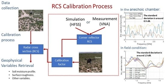
1. Introduction
There is a growing interest in using uncrewed aerial vehicles (UAVs) as a tool for remote sensing, complementing existing platforms such as satellites, high-altitude airplanes, and aerostats [
1]. By bridging the gap and addressing the inherent limitations of other platforms, UAVs bring unique advantages in terms of mobility, low cost, and ease of deployment. The capability of UAVs to achieve high spatial and temporal resolution with a short revisit time surpasses other existing platforms. Radar systems mounted on UAVs can improve the accuracy of the collected data for the Essential Variables (EVs) and essential climate variables (ECVs) such as soil moisture, snow depth, surface water levels, and water table [
2,
3]. As the UAVs pave the way for advancing climate studies and environmental monitoring, they come with challenges, particularly in calibration. Addressing the calibration challenges enables utilizing the full potential of radar mounted on a UAV.
Radar cross section (RCS) calibration of the radar is essential for producing scientific products. The calibration accuracy directly influences the accuracy of the retrieved product. The common and low-cost approach to calibrate the radar is to use a corner reflector (CR) [
4]. The CR has been and is planned to be used to calibrate various synthetic-aperture radar (SAR) missions, including NISAR, UAVSAR, and SWOT missions [
5,
6]. The radar calibration literature describing the use of trihedral and other CRs is quite extensive. For example, Sarabandi et al. provided a CR design for SAR calibration [
7]. Further research by Doerry has explored the use of other objects for calibration, including different shapes of CR [
8]. Doerry also studied the impact of the ground in the CR calibration process. Additionally, Gibert et al. utilized the CR to calibrate radar altimeters [
9]. Toledo et al. have successfully calibrated a frequency modulated continuous wave (FMCW) radar using a CR mounted on a mast [
10]. Notably, all these efforts for calibrating the radar were in the far-field region of the object and the antenna.
Our system is a Software-Defined Radar (SDRadar) mounted on a hexacopter UAV [
11]. It is an ultra-wideband (UWB) system with more than a 1 GHz bandwidth with the lowest frequency set at
GHz. The UAV was flown at a height of around 10 m above ground level (AGL). The UAV’s height was chosen to be relatively close to the ground to reduce the wave propagation loss in the air and the antenna’s footprint. For external calibration, we used a trihedral CR with a size of
m. The size was selected to be large and easy to assemble. Flying the UAV at the above-mentioned height, and given the range of operational frequencies used, places the antenna in the near-field region of the CR. There are four main challenges with the calibration process of our system using this CR. First, the small size of the CR results in the physical optics (PO)’ approximation being invalid. Second, the radar antenna is in the near-field region of the CR. Therefore, the far-field approximation of the CR is not applicable. Third, the ground RCS relative to the CR RCS ratio is not insignificant and cannot be ignored. Lastly, the calibration has to be valid over a large bandwidth, which is different from most of the existing radar systems. Overcoming these challenges is crucial in achieving accurate calibration of our system.
There are a small number of investigations of the near-field RCS for a few canonical objects. They predominantly rely on the PO approximation for the near-field RCS calculation. For example, Ruch et al. provided the approach to compute the near-field RCS for 2D objects [
12] and Chengjin et al. derived the near-field RCS for a perfect electric conductor (PEC) plate, two-side CR reflector, and a ship modeling the wave as spherical waves and using the PO approximation [
13]. Similarly, Karaca et al. show the result for near-field RCS for a PEC sphere illuminated by a dipole antenna [
14]. Bourlier et al. compute the near-field RCS of a PEC plate and disk using the PO approximation, demonstrating RCS behavior as the object approached the far-field region [
15,
16]. In addition, Dogaru uses AFDTD software to compute the near-field RCS and compare it with theoretical near-field RCS derived from PO approximation for a square plat [
17]. All these investigations assume PO approximation, which is not valid for our problem. Furthermore, most of the investigations focused on 2D objects.
The application for near-field RCS computation extends beyond radar calibration, including various applications such as automotive radar and terahertz radar systems. Automotive radar often encounters targets in close proximity to the radar [
18], while the terahertz radar systems operate in the near-field region [
19]. Elfrgani et al. computed the near-field RCS for automotive radar operating at W-band using Altair Feko software [
18]. Xiao et al. proposed a generalized radar range equation to incorporate the near-field case [
19]. In these scenarios, where the radar is in the near-field region of the object, the traditional method for calculating the RCS with the far-field assumption is invalid. The near-field RCS must be considered to calibrate the radar system or analyze the scatter.
This paper presents a calibration process for UWB SDRadar using a trihedral CR in the near-field region. To achieve this, we develop a simulation framework for an object in the near-field region using HFSS, version 2021 R1. The simulation uses the hybrid solver in HFSS software, where the antenna is modeled using the finite element method (FEM) solver, and the CR is modeled using the integral equation (IE) solver [
20]. The HFSS simulation is validated with an anechoic chamber measurement of the CR using a vector network analyzer (VNA). Furthermore, the SDRadar calibration performance was studied for both the anechoic chamber and the field measurements.
The rest of the paper is organized as follows: the approach to solving the problem is discussed in
Section 2. In
Section 2.3, the near-field CR RCS is presented using both VNA measurement in the anechoic chamber and HFSS software simulation. The SDRadar calibration performance is discussed in
Section 3 for both the anechoic chamber and field data. Finally,
Section 5 provides our conclusions.
2. Materials and Methods
In this section, we outline our approach to calibrating the SDRadar. We begin with an overview of our system and the CR design. Subsequently, our electromagnetic field operating regions are discussed. Lastly, our method to calibrate the SDRadar is presented.
Our SDRadar system studied here is installed on a drone [
11]. The SDRadar is implemented on universal software radio peripheral (USRP) E312. The transmitted wave is a synthetic wideband waveform (SWW) with a bandwidth of more than 1 GHz [
21]. The antennas are RFSPACE TSA600, with a 34 cm separation between the transmitter and receiver antennas [
22].
The CR is a triangular trihedral CR with a side size of
m. It was built using 5 mm thickness plywood sheets with copper tape to reduce the weight of the CR. This made it easy to deploy and install in the field site. The CR is shown in
Figure 1 during flight operations. Other calibration targets, such as a sphere, were not considered due to their construction complexities and associated costs. Building a sphere large enough to be effective within the operational frequency range would have been challenging, costly, and difficult to deploy in the field. Moreover, it would have a significantly smaller RCS value compared to the triangular trihedral CR.
There are three electromagnetic field regions for the radar: reactive near-field, radiating near-field (Fresnel), and far-field (Fraunhofer) regions. The far-field region is commonly defined as the maximum phase error of less than
and it is commonly defined as [
23]
Note that
D is the largest dimension in the object,
R is the distance to the object, and
is the wavelength. The reactive field predominates in the reactive near-field region. Objects present in this vicinity affect and modify the antenna radiation. The reactive near-field region is commonly defined as
These regions’ boundaries are not strict. The maximum length in the CR is
m, and the UAV operates from 4 m to 10 m AGL, which is the distance from the radar to the target. Based on our UAV height, the size of the CR, and the operating frequency range, we are in the radiating near-field (Fresnel) region. The three regions for the CR with distance are shown in
Figure 2.
The goal of calibrating the radar is to convert the radar digital readings to RCS values. In other words, it is to determine the RCS value measured by the radar. This calibration can, therefore, be used to obtain the absolute RCS for discrete targets as well as for distributed surfaces. The distributed target scattering responses all enter the radar antenna footprint and are added to form a single RCS value. The SDRadar measurements are first converted to a power count via a pulse compression algorithm, which is related to the RCS [
11]. The calibration process we propose here estimates a calibration factor that converts the received power count by the radar to an RCS value. Since our system is UWB, the calibration factor is a function of frequency. The radar range equation with near-field RCS consideration is
Note that
is the received power,
is the transmitter power,
is the transmitted antenna gain,
is the received antenna gain,
is the wavelength,
R is the distance between the target and the radar, and
is the near-field RCS of any target, and it is a function range. The only distinction between our approach and the traditional far-field radar range equation is that the RCS is a function of the range, unlike in the far-field radar range equation where the RCS is independent of the range. We did not consider the antenna gain to be range-dependent since we are not operating in the reactive near-field region. Our assumption is that any range-dependent effects are included within the near-field RCS, and other antenna parameters are independent of the range. The calibration factor combines all the constants and variables in (
3) that are independent of the range, and it is defined as
Note that
is the RCS of a known target. The calibration factor can be applied to the received power count to determine the RCS value as follows:
The calibration process requires a target with a known RCS value; in our case, the target is the CR. The near-field RCS of the CR is computed in the next section. The calibrations were assessed for two cases: in the anechoic chamber and in the field conditions. The calibration processes for the two cases are discussed in the rest of this section, while the calibration performance assessment is presented in
Section 3.
2.1. Anechoic Chamber
The calibration measurement in the anechoic chamber is ideal since the reflection from the background is minimized. The processing steps for the received signal by the SDRadar are outlined as follows:
Sky-calibration removal: This step was performed to reduce the direct path between the transmitting (Tx) and receiving (Rx) antennas.
SWW construction: Pulse compression and construction of the SWW signal.
Range-gating: Apply a window around the reflected echo from the CR.
Range compensation: Compensate for the free space travel time.
Frequency domain conversion: Apply a discrete Fourier transform (DFT) to the reflected signal from the CR.
From (
3) and (
4), the calibration factor can be computed as
Note that
,
, and
are functions of frequency because our system is UWB.
2.2. Field Site
Calibrating the SDRadar in field conditions presents unique challenges due to the presence of the ground. Two approaches were considered that take into account the presence of the ground. Each approach has different approximations and assumptions to the ground model to reduce the complexity of the problem. Although our operation region is the near-field, we assume a far-field model for the ground to reduce the computation time and complexity. The first approach assumes we only observe the CR since the specular point is on the CR, not on the ground [
4]. Therefore, its contribution is much less than the CR and can be ignored. The second approach includes the ground, modeled as a one-layer medium with a random rough surface. Another approach, which assumes a near-field operating region, is to include the ground as a multi-layer medium with roughness in the electromagnetic simulation. This was not considered since it requires knowledge of subsurface layer properties (not available) and very large computational resources.
The first approach for computing the calibration factor was the same as the anechoic chamber experiment since the effect of the ground was not present. For the second approach, we assume the reflected power from the ground is added algebraically with CR reflection. The calibration factor for the second approach with the RCS of the ground is therefore expressed as
Note that
is the RCS of the ground which is defined as
where
is the normalized RCS of the ground, and
is the antenna footprint. The integral was numerically evaluated with the footprint and discretized into half-degree cell sizes. The H- and V-polarizations were assumed to be equally distributed within the antenna footprint, each contributing half of the total power. The 3 dB beam width of the antenna was used to compute the antenna footprint as an ellipse, defined as
Note that
and
are the azimuth and elevation 3 dB beam widths of the antenna. The normalized RCS of the ground is modeled as a single-layered medium with random roughness. The small perturbation method (SPM) was used to model the surface roughness [
24]. The soil dielectric constant was modeled using the generalized refractive mixing dielectric model (GRMDM) [
25]. The soil moisture was measured near the CR via the Soil moisture Sensing Controller and oPtimal Estimator (SoilSCAPE) in situ sensor network [
26,
27].
2.3. RCS of the Corner Reflector
The RCS value of the CR is required to calibrate the SDRadar. The sections present the calculations of the CR RCS for both the far-field and near-field conditions using HFSS. Moreover, the near-field RCS of a CR was measured in the anechoic chamber and compared with the HFSS results. In addition, the antenna parameters—gain, pattern, and reflection coefficient—were measured in the anechoic chamber, which is a needed step to compute the measured near-field RCS and understand the results.
2.4. HFSS Simulation for the Corner Reflector RCS
2.4.1. Far-Field RCS of CR
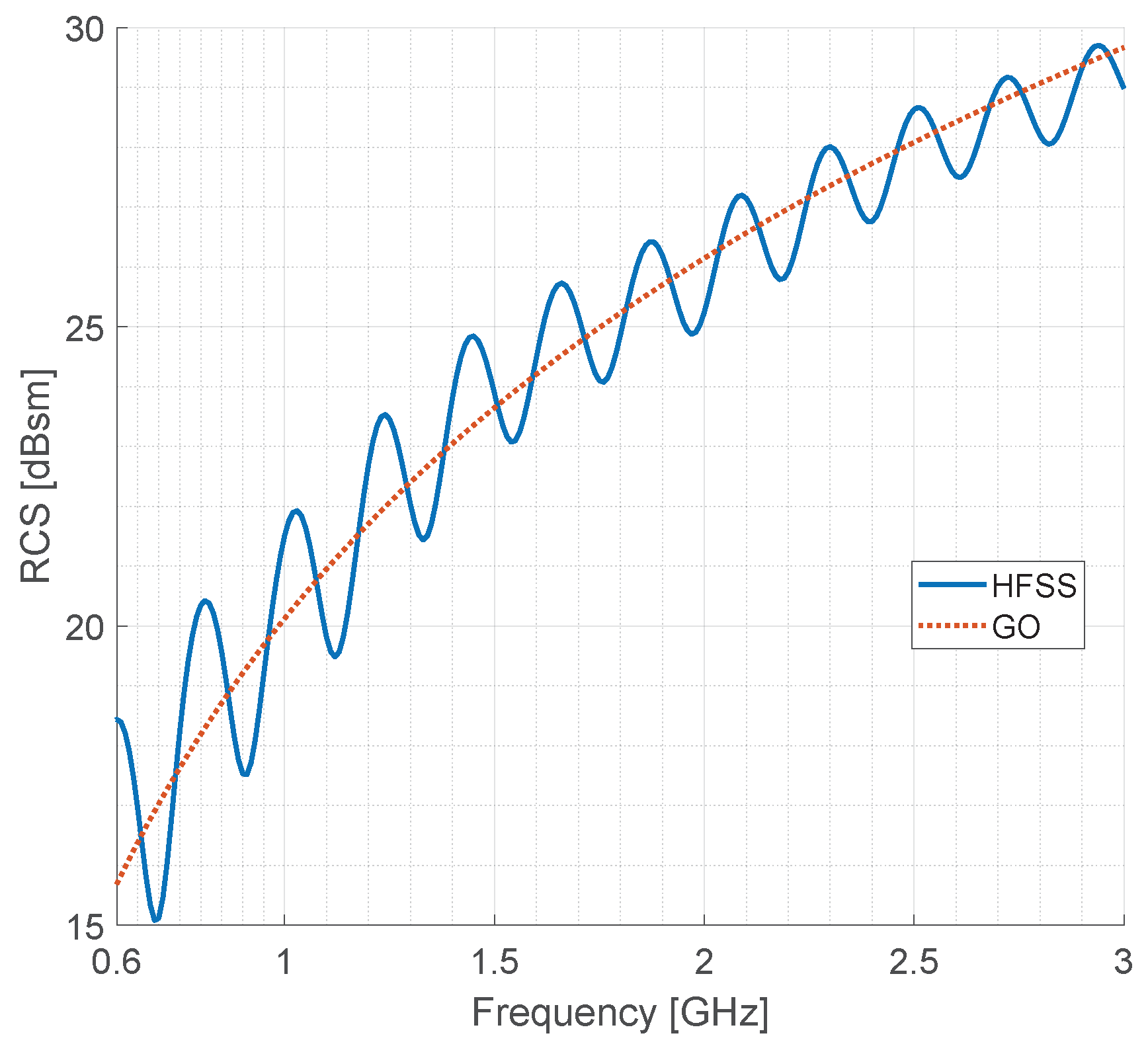
The far-field RCS is used as a comparative benchmark against the near-field RCS. The geometry of the triangular trihedral CR can be seen in
Figure 3. It is common to use the geometric optics (GO)’ approximation to compute the CR RCS. The GO approximation is valid when the CR size is significantly larger than the wavelength, typically by a factor of ten. The far-field RCS of the CR using a GO approximation near the symmetry axis is [
8,
12].
The far-field RCS peak using the GO approximation is located at
and
. The value of the far-field RCS at the peak location is
A more accurate approach to compute the far-field RCS is using the method of moments (MoM), which requires more computational power, but it is valid regardless of the CR size and the wavelength. The HFSS software was used to compute the far-field RCS of the CR. The CR is modeled as a PEC with a 1 mm thickness.
The far-field RCS as a function of frequency is shown in
Figure 4. The RCS values oscillate with frequency, and the amplitude of the oscillation decreases as the frequency increases. Notably, the interval between the oscillation peaks remains constant, and it is inversely proportional to the CR size. The GO approximation should be valid around 3 GHz (wavelength of 10 cm), where the difference between the MoM and GO approximation is very small. These observations of the RCS oscillation and the difference between the MoM and GO approximation are aligned with the findings in [
28] for a smaller CR.
Figure 5 illustrates the far-field RCS as a function of the elevation angle. The far-field RCS peak using the MoM varies with frequency but occurs at around
, the same as predicted by the GO approximation. This aligns with our expectation that the GO approximation may not capture all the behavior of the CR far-field RCS, but becomes more accurate as its assumptions become more valid.
2.4.2. Near-Field RCS of CR
Given that the SDRadar is in the near-field region of the CR, the far-field approximation is inapplicable and we need to compute the near-field RCS. The RCS of the CR is defined using the radar range equation as follows:
The HFSS simulation can account for all of the quantities in the equation. The antenna gain can be computed using infinite sphere radiation in HFSS. Simulating the whole domain is unfeasible, given the large simulation domain size. To address this, the HFSS hybrid solver was used. It divides the problem into two simulation components: antennas and the CR. The antenna region is solved using FEM, while the CR is solved using the IE solver, which uses the MoM. HFSS computes the S-parameters related to the transmitted and received power given by the following equation:
Note that
is the scattered field S-parameters from the CR between the transmitter and receiver antennas.
One of the methods to compute the scattered field S-parameters from CR is to use the background and the total S-parameters. The background is the simulation of the antennas without the CR, while the total is the simulation of the antennas with the CR, as shown in
Figure 6. The background scene consists of two RFSPACE TSA600 antennas with a 34 cm separation. While the total scene consists of the antennas and the CR position at
and
, respectively. The scattered field S-parameters from the CR is given by
Note that
and
are the background and total S-parameters, respectively.
The near-field RCS of the CR from
GHz to 3 GHz is shown in
Figure 7. The data were filtered using a moving medium and mean filters to mitigate computational noise. The frequency resolution was 10 MHz, and the window size of the moving medium and the mean filters were set to three and five, respectively. The near-field RCS values increase with range as they become closer to the far-field approximation. Similarly, the difference between near-field RCS for different ranges becomes smaller as the frequency decreases and becomes closer to the far-field approximation. Moreover, it was observed that the near-field RCS values become smaller than the far-field RCS as the frequency increases, diverging from the far-field approximation.
2.5. Antenna and Corner Reflector RCS Measurements in the Anechoic Chamber with VNA
2.5.1. Far-Field Antenna Measurement
Measuring the antenna parameters is essential for computing the CR RCS and understanding the results. Three parameters of the RFSPACE TSA600 antenna were measured in the anechoic chamber: reflection coefficient, gain, and antenna pattern. The measurements of the reflection coefficient and antenna pattern are needed to understand the trends in the results, while the antenna gain is needed to compute the RCS of the CR. The three-antenna method was used to measure the antenna gain to accommodate any potential variations arising from the manufacturing process [
23]. All three antennas were RFSPACE TSA600 mounted on the payload structure. The distance between the antennas was
m, ensuring the antennas are in the far-field region. The antennas’ gain are shown in
Figure 8. There is a slight difference in the gain between the antennas, which was expected due to the manufacturing variations.
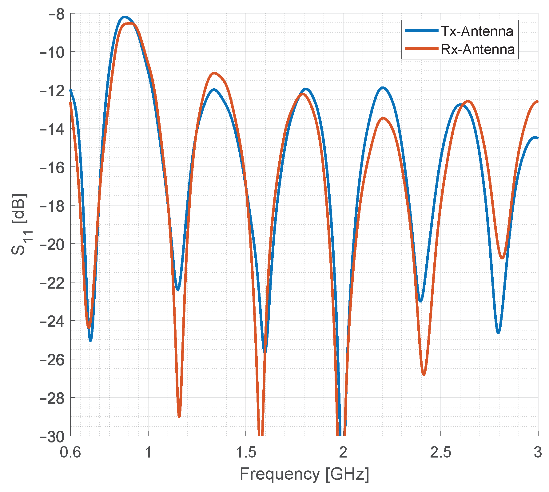
The reflection coefficient of the antennas mounted on the payload structure is shown in
Figure 9. The reflection coefficient is larger than
dB in the frequency region from
GHz to 1 GHz. This high reflection coefficient could adversely affect the calibration performance, such as a poor signal-to-noise ratio.
The elevation antenna pattern of the RFSPACE TSA600 is shown in
Figure 10. The measurement was with the RFSPACE TSA600 antenna alone, without the payload structure. Two RFSPACE TSA600 antennas were used in this measurement, with the distance between the antennas being
m, ensuring the antennas are in the far-field region. The antenna pattern has high side lobes and grating lobes in the frequency region from
GHz to
GHz. These high side lobes, grating lobes, and the high reflection coefficient in the frequency region from
GHz to 1 GHz pose a potential limitation in the ability to calibrate the SDRadar in this frequency region.
2.5.2. CR RCS Measurement
Most of the literature on radar calibration predominantly focuses on measuring the RCS of a passive external target in the far-field region [
28,
29,
30,
31,
32]. A calibration curve is then built as a function of the incidence angle. Moreover, time-gating around the target is sometimes applied to remove the background and other effects. The standard calibration targets are usually chosen to be large compared to the operating wavelength. In our case, it is notable that the size of the standard passive calibration targets with known RCS is very large for a large portion of the UWB of operating frequencies. Therefore, the standard version of this approach is impractical for our application.
Our methodology for computing the near-field RCS from anechoic chamber measurements is similar to our method of computing the RCS in HFSS. We use the measured antenna gain and the observation distance to compute the near-field RCS. The processing steps to compute the near-field RCS are as follows:
Time-domain total signal: The S-parameters measured by the VNA are converted to the time domain.
Time-domain scattered signal: The first reflection from the CR is time-gated to remove the background and multi-bounce reflections.
Scattered field S-parameters: The time-domain signal is converted back to the frequency domain.
Near-field RCS: The near-field RCS is computed using (
12).
The SDRadar system and the CR are positioned in the anechoic chamber, as shown in
Figure 11. The VNA is connected to the transmitter and receiver antennas of the SDRadar system. The signal in the time domain is shown in
Figure 12, where the direct path between the transmitter and receiver antennas is clear. Moreover, the double-bounce and third-bounce are noticeable. Time-gating the first reflection from the CR is essential to isolate the scattered field from CR from the other reflections.
The near-field RCS of the CR measured by the VNA is shown in
Figure 13. The near-field RCS behavior is similar to the near-field RCS simulated by HFSS. However, it is noticeable that the RCS value below 1 GHz has an unexpected behavior. This is due to the antenna pattern of the RFSPACE TSA600 antenna having grating lobes, high side lobes, and a high reflection coefficient at the frequency range below 1 GHz. The grating lobes could create an effect similar to a varying incident angle that changes with distance and frequency. This effect was not observed in the HFSS simulation since the simulated RFSPACE TSA600 antenna does not have this behavior. The frequency region below 1 GHz should therefore be excluded due to the compound adverse effects of grating lobes, high side lobes, and high reflection coefficients.
2.5.3. Comparison of CR RCS Simulation with Measurement
The comparison between the near-field RCS measured using the VNA and simulated in HFSS is shown in
Figure 14. The differences observed for frequencies below 1 GHz are expected due to the antenna pattern and the reflection coefficient, as discussed previously. In the frequency range outside of this band, the difference becomes higher as the SDRadar system becomes closer to the CR. This is mostly due to the imprecise fabrication of the CR and alignment errors between the SDRadar system and the CR. The difference between the VNA and the HFSS can be reduced by improving the CR fabrication and minimizing the deforms in the CR. Moreover, the stands for CR and the payload can be improved to ensure better alignment and minimize errors due to misalignment.
3. Results
The calibration performance was studied in the anechoic chamber and then also using actual field data. The performance was compared for three cases of computing the CR RCS: far-field RCS using MoM, near-field RCS computed using HFSS, and near-field RCS measured in the anechoic chamber.
3.1. SDRadar Calibration in the Anechoic Chamber
The calibration process in a controlled environment, such as the anechoic chamber, is ideal due to the minimization of background reflection, misalignment, and the absence of vibration. These conditions facilitate a precise calibration compared to the field conditions. The measurement setup is the same as that of the CR RCS measurement with antennas connected to the SDRadar. The waveform bandwidth was more than 2 GHz, starting at 675 MHz.
The near-field RCS is a function of the range, but the calibration factor is independent of the target’s distance. Therefore, the calibration factor should be constant for different ranges. We conducted the calibration experiment for seven different distance values from m to m. The calibration factor was computed for three RCS calculation methods: near-field RCS computed using HFSS, near-field RCS measured via VNA, and far-field RCS. The near-field RCS measured via VNA does not have the same range value as the calibration experiment. A linear interpolation was used to compute the near-field RCS measured via VNA at the calibration experiment range values.
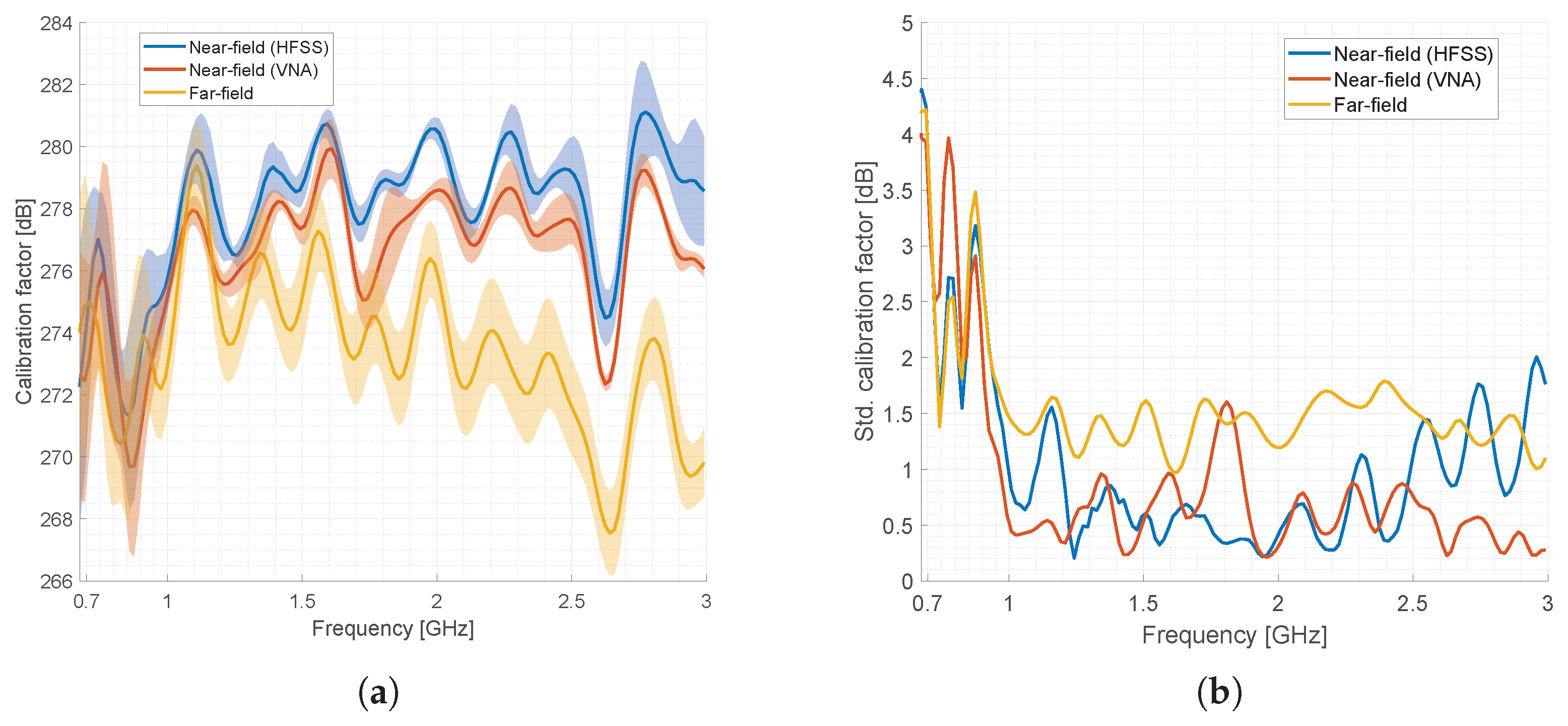
The estimated calibration factor is shown in
Figure 15a, where the solid line is the mean of seven different measurements, and the shaded area presents one standard deviation. The standard deviation of the calibration factor for the three RCS cases is shown in
Figure 15b.
3.2. SDRadar Calibration Using Field Data
Calibrating the SDRadar in the field poses additional challenges due to the effect of the ground and more errors in aligning the drone with the CR. The field measurements were conducted on 17 August 2022 at the Lucky Hills site within the Walnut Gulch Experimental Watershed, Arizona, USA [
33,
34]. The area is covered by small shrubs, typically less than a meter, and has moderate topography. The surface roughness in the measurement area was measured, and it had a root mean square (RMS) value of around
cm [
35]. The measured soil moisture near the CR value was 0.17 m
3/m
3. There were 64 unique acquisitions of the CR with the drone’s height varying between 4 m and
m. The transmitted waveform was SWW with a 1 GHz bandwidth.
The calibration factors are shown in
Figure 16a for the two approaches with the CR RCS computed via three methods: near-field in HFSS, measured near-field in the anechoic chamber, and far-field. The solid line is the mean of 64 measurements and the shaded area presents one standard deviation. The standard deviation of the calibration factors is shown in
Figure 16b.
Given the impact of ground effects and misalignment on the calibration error, we excluded some measurements that had a wide main lobe or high side lobe. The main lobe width threshold was
m, while the side lobe threshold was 10 dB. The number of measurements that passed the thresholds was 24. The calibration factors and the standard deviation for the measurements that passed the thresholds are shown in
Figure 17a,b, respectively.
4. Discussion
4.1. SDRadar Calibration in the Anechoic Chamber
For all of the cases, the standard deviation is high below 1 GHz. As discussed in the previous section, this is expected due to the antenna pattern and the reflection coefficient. The far-field RCS case has a standard deviation around
dB, which is considered to be high compared to modern-day radar calibration requirements [
5]. The standard deviation for the near-field RCS computed via HFSS grows rapidly beyond
GHz. This might be due to increased simulation inaccuracy at high frequency. In addition to these regions, both cases of the near-field RCS have a standard deviation around
dB, which meets or exceeds typical radar calibration requirements, especially for soil moisture applications. This is noteworthy given that the SDRadar system power varies with a standard deviation around
dB during the acquisition time. The near-field RCS measured via VNA and the simulated values from HFSS follow similar patterns, and there is a difference between them of approximately
dB. This difference is due to CR and SDRadar alignment errors and fabrication defects in the CR.
4.2. SDRadar Calibration Using Field Data
As discussed earlier, the frequency region below 1 GHz is ignored because of the observed issues in the antenna pattern and reflection coefficients. The difference between the two approaches is very small and negligible because the ground is not in the specular point, and the CR RCS is at least 8 dB higher than the ground RCS. The calibration factor pattern is similar to the anechoic chamber calibration factor. The standard deviation is high for all of the different methods of computing the CR RCS. This is likely due to factors such as CR misalignment and the presence of the ground.
Excluding the measurements with a wide main lobe or high side lobe improved the standard deviation of the calibration factor, which is expected since it reduced the impact of the ground and the CR misalignment. Still, this standard deviation is higher than the anechoic chamber measurements. Considering the calibration factor pattern in the anechoic chamber measurements, we can observe the near-field RCS is the best estimated calibration factor in the field.
We anticipate differences between the calibration factor obtained in the field measurements and the anechoic chamber measurements due to a few factors. There is a difference in the mounting setup of the payload: in the anechoic chamber, it is mounted on a stand, whereas in the field, it is mounted on the UAV in the field. This should affect the sky-calibration removal step, which results in a different calibration factor. Secondly, the waveform bandwidth is different, which should change the processing gain, leading to a change in the calibration factor. Moreover, the output power from the SDRadar system could change by around 1 dB from day to day, with no change in the setup. These factors collectively contribute to the expected differences in the calibration factors between the field and the anechoic chamber measurements.
Several strategies may improve the calibration of the SDRadar in the field site and will be explored in our future work. One approach is to elevate the calibration target above the ground, where range gating around the object can be applied to separate the object from the ground. Another strategy is to use a simpler calibration object with narrow boresight, so that the measurements with misalignment can be excluded easily. A suggested object is a metal sheet, which is easy to deploy and has the ability to arrange multiple sheets to form a larger surface. It has less RCS compared to the CR, but the benefits surpass the weaknesses.
The precision of calibration is impacted by several factors related to the UAV, such as uncertainties in its position, orientation, and vibrations. Subsequently, in the geophysical variables’ retrieval, these calibration errors are compounded with the UAV’s inherent uncertainties, further affecting the accuracy of the retrieval product. Several strategies could be applied to mitigate the UAV uncertainties. One effective approach is to utilize specific time-domain signal features, such as the compressed time-domain pulse main lobe width and side lobe level, to exclude the observation with high UAV uncertainties. This selective exclusion process refines the observations used in the geophysical variables’ retrieval. Consequently, this approach should improve the overall retrieval accuracy.
5. Conclusions
This paper presents a framework and process to calibrate SDRadar with a UWB waveform in the near-field region. Moreover, we demonstrate the need for near-field RCS for calibration and the invalidity of far-field RCS in scenarios where the system operates in the near-field region. In addition, the framework and process have been shown for computing the near-field RCS using HFSS for an object with specific antennas.
The near-field RCS of the CR is computed via HFSS and measured in the anechoic chamber. The near-field RCS of the CR becomes closer to the far-field RCS as the operation region becomes closer to the far-field. There was some discrepancy between the simulated RCS and the measured RCS, most probably due to manufacturing defects in the CR, misalignment of the CR, and antenna pattern defects.
Employing the near-field RCS significantly reduced the standard deviation of the calibration factor, achieving a standard deviation around dB when the calibration was performed in the anechoic chamber. In the case of the field experiment where the effect of the ground is present, the standard deviation of the calibration factor was around dB. This is mostly due to misalignment between the drone and the CR and the effect of the ground.
Several practical considerations can improve the calibration process in the field site and will be explored in our future work. First, we can elevate the calibration object above the ground. This allows for the separation of the ground reflection from the calibration object reflection. Second, we can use a calibration object that is less susceptible to misalignment. A suggested object is a square metal sheet elevated above the ground. This should improve the calibration performance, bringing it closer to the performance observed in the anechoic chamber measurement.
Radar Calibration is a crucial initial step toward retrieving valuable scientific products, specifically soil moisture and other important EVs, which are typically formulated as inverse problems using the observed scattering RCS, estimating geophysical variable values that minimize the difference between such observations and the corresponding theoretical predictions. Radar calibration allows for exploring the full potential of our UWB SDRadar system, broadening its application. Furthermore, it enhances the capabilities of the UAV platform, enabling it to augment and complement scientific products of other existing remote sensing platforms.


