
Global and Multiscale Aggregate Network for Saliency Object Detection in Optical Remote Sensing Images


1
School of Computer and Cyberspace Security, Hebei Normal University, Shijiazhuang 050024, China
2
Key Laboratory of Intelligent Perception and Image Understanding of Ministry of Education, Xidian University, Xi’an 710071, China
*
Author to whom correspondence should be addressed.
Remote Sens. 2024, 16(4), 624; https://0-doi-org.brum.beds.ac.uk/10.3390/rs16040624
Submission received: 8 December 2023
/
Revised: 5 February 2024
/
Accepted: 5 February 2024
/
Published: 7 February 2024
(This article belongs to the Special Issue Object Detection and Information Extraction Based on Remote Sensing Imagery)
Abstract
:Salient Object Detection (SOD) is gradually applied in natural scene images. However, due to the apparent differences between optical remote sensing images and natural scene images, directly applying the SOD of natural scene images to optical remote sensing images has limited performance in global context information. Therefore, salient object detection in optical remote sensing images (ORSI-SOD) is challenging. Optical remote sensing images usually have large-scale variations. However, the vast majority of networks are based on Convolutional Neural Network (CNN) backbone networks such as VGG and ResNet, which can only extract local features. To address this problem, we designed a new model that employs a transformer-based backbone network capable of extracting global information and remote dependencies. A new framework is proposed for this question, named Global and Multiscale Aggregate Network for Saliency Object Detection in Optical Remote Sensing Images (GMANet). In this framework, the Pyramid Vision Transformer (PVT) is an encoder to catch remote dependencies. A Multiscale Attention Module (MAM) is introduced for extracting multiscale information. Meanwhile, a Global Guiled Brach (GGB) is used to learn the global context information and obtain the complete structure. Four MAMs are densely connected to this GGB. The Aggregate Refinement Module (ARM) is used to enrich the details of edge and low-level features. The ARM fuses global context information and encoder multilevel features to complement the details while the structure is complete. Extensive experiments on two public datasets show that our proposed framework GMANet outperforms 28 state-of-the-art methods on six evaluation metrics, especially E-measure and F-measure. It is because we apply a coarse-to-fine strategy to merge global context information and multiscale information.
1. Introduction
Salient Object Detection (SOD) endeavours to emulate the human visual system, empowering computers to identify the most compelling objects or regions within a given scene [1]. Serving as a pivotal image preprocessing step, salient object detection finds diverse applications, including object segmentation [2], image relocation [3], image retrieval, classification [4], image compression, and target recognition.
The conventional methodology for salient object detection involves hand-crafted features [1], yet its efficacy and precision are suboptimal. With the advent of deep learning, researchers have incorporated Convolutional Neural Networks (CNN) into computer vision [5], resulting in superior outcomes compared to hand-crafted features [6]. Different conceptualisations have been proposed, such as multiscale, attention, and edge guidance. Recently, salient object detection has garnered increased attention, manifesting in various branches such as salient object detection for natural scene images (NSI-SOD) [7], RGB-D salient object detection [8,9], RGB-T salient object detection, and video salient object detection. There are other tasks similar to salient object detection in computer vision, such as object detection, novelty detection, anomaly detection, and clustering. Object detection is used to detect and classify all objects in an image. It usually outputs a bounding box around the detected object and the corresponding class label [10]. Salient object detection focuses on identifying visually salient objects or regions, while object detection focuses on detecting and classifying multiple instances of different classes. Novelty detection and anomaly detection are both recognition problems that deal with rare or abnormal instances. However, novelty detection focuses on detecting new patterns [11]. Meanwhile, anomaly detection aims to detect instances that are significantly different from the norm, which are usually used in network intrusion, medical diagnosis, and other fields [12]. Clustering divides data into clusters based on similarity or proximity between them and aims to discover natural groupings or clusters in the data [13]. Unlike other tasks, clustering does not require prior knowledge of the class labels.
This study is specifically dedicated to a distinct application of salient object detection, salient object detection in optical remote sensing images (ORSI-SOD). In optical remote sensing images, salient objects refer to the obvious or prominent features in the image that stand out from the surrounding environment, including colour, brightness, texture, shape, and other important attributes. Salient objects are often meaningful for specific applications or analysis. For example, in urban planning, the salient objects can be buildings, roads, or other infrastructure. In topographic analysis, the salient objects can be rivers, farmlands, and islands. Detecting salient objects is critical in processing and analysing optical remote sensing images because it can focus attention on areas of interest and facilitate more efficient data decisions.
Distinctive features of optical remote sensing images relative to natural scene images include:
- (1)
- Optical remote sensing images offer surface information encompassing cities, farmland, rivers, buildings, and roads, reflecting a diversity of object types [14].
- (2)
- Objects in optical remote sensing images exhibit varying sizes, e.g., ships, aeroplanes, bridges, rivers, and islands, signifying diversity in target size [14].
- (3)
- The background of an optical remote sensing image may comprise intricate textures and structures, surpassing the complexity of a natural image [14].
Consequently, tools or methodologies for salient object detection in natural scene images may not be directly applicable to ORSI-SOD. Research in ORSI-SOD typically adopts a CNN-based encoder-decoder structure, with VGG [15] and ResNet [16] as the backbone network. Additionally, related studies have introduced modules to enhance model accuracy, including the attention module [17], multiscale module, and edge guidance module [18]. However, CNN-based network models predominantly focus on the convolution of local features and lack the capability to learn remote relations, resulting in issues such as misdetection, omission of salient objects, and inaccuracies. This limitation is particularly pronounced in the context of ORSI-SOD, where the predicted results lack global structural consistency.
This study replaces the CNN backbone with the Pyramid Vision Transformer v2 (PVT-v2) to address the challenges above and introduces a novel salient object detection method known as the Global and Multiscale Aggregate Network (GMANet) for ORSI-SOD. GMANet is specifically tailored for Optical Remote Sensing Images (ORSI) and comprises a PVT-v2 encoder, a Global Guidance Branch (GGB), an Aggregation Refinement Module (ARM), and a Dense Decoder (DD). Notably, the GGB incorporates four densely connected Multiscale Attention Modules (MAM) to address the identified effectively.
The key contributions of this study are as follows:
- (1)
- This research replaces traditional CNN-based ResNet or VGG with a transformer-based backbone network, PVT-v2, to enhance the comprehensiveness of salient regions. Unlike CNN-based methods that primarily capture local information, transformer-based approaches excel in learning remote dependencies and acquiring global information. The proposed encoder-decoder architecture includes a PVT-v2 encoder for learning multiscale features and a DD for hierarchical feature map decoding. At the same time, a Global Guidance Branch is designed on the encoder.
- (2)
- The study introduces the MAM, recognising the challenge of large variations in object scales within optical remote sensing images. This module adeptly extracts multiscale features and establishes densely connected structures for the GGB. The GGB leverages four MAM modules to generate global semantic information, guiding low-level features for more precise localisation.
- (3)
- The ARM is innovatively proposed in this study to amalgamate global guidance information with fine features through a coarse-to-fine strategy. Leveraging global guidance information ensures accurate localisation of salient objects, capturing the complete structural context, while the incorporation of fine features augments details in the preliminary saliency map.
This investigation executed a series of comparative experiments, utilising the GMANet model, against 28 state-of-the-art methods on two publicly available ORSI-SOD datasets. The outcomes of these experiments reveal the heightened competitiveness of the GMANet proposed in this study in comparison to previously introduced methodologies. Particularly noteworthy is the superiority of the proposed method, demonstrating a 3.50% improvement in terms of over the second-ranking method. A comprehensive evaluation across all methods on the ORSSD dataset highlights the distinctiveness of the method presented in this study. It stands out as the singular approach to attaining exceeding 0.86, surpassing 0.88, and exceeding 0.97. This substantiates that the proposed method contributes to enhanced object accuracy and area completeness relative to alternative methodologies.
The subsequent sections of this paper are organised as follows: Section 2 provides an extensive review of the pertinent literature on ORSI-SOD. Section 3 offers a detailed exposition of the GMANet components. In Section 4, a thorough analysis of the experimental results and ablation experiments is conducted. Finally, Section 5 presents concluding remarks and a comprehensive summary of the study.
2. Related Work
This section provides a comprehensive review of research outcomes in the domain of the NSI-SOD and ORSI-SOD. The investigation spans both traditional and CNN-based methodologies.
2.1. Traditional Methods for NSI-SOD
Pioneering the field, Ltti et al. [19] introduced the initial computer vision attention model founded on the centre-surround disparity mechanism for localisation. Traditional NSI-SOD approaches predominantly rely on hand-crafted features [1], with three primary categories: unsupervised, semi-supervised, and supervised methods. While the majority are unsupervised [19,20,21,22,23,24], there are fewer semi-supervised [25] and supervised methods [26]. Notable examples include Kim et al.’s extension [22] of the SOD method based on high-dimensional colour transformations and Zhou et al.’s iterative semi-supervised learning framework [25]. Some studies [20,21] used techniques like random walk and ranking. The random walk algorithm is able to compute a saliency score for each pixel. The ranking algorithm ranks the images according to the saliency score of the pixels. In [22], a high-dimensional colour transform is used to map the colour of image pixels to a high-dimensional space, which can better capture the differences and relationships between colours. Liang et al. [26] employed support vector machines for feature selection through supervised learning. Although traditional methods may lack generalisability in novel scenarios, they form the foundational basis for subsequent methodologies.
2.2. CNN-Based Methods for NSI-SOD
CNN-based NSI-SOD methods have surpassed the limitations of traditional approaches [1]. These CNN-based methods predominantly operate through supervised learning, diverging from their traditional counterparts. Enhancements to model accuracy include Zhao et al.’s introduction of an edge-aware network [18], Liu et al.’s design of a pooling-based module [27], and the widespread integration of attention mechanisms [17,28]. The use of various loss functions, such as the IoU loss introduced by Ma et al. [29] and SSIM loss by Qin et al. [30], further refines the supervised learning process. GateNet proposed Folded Atrous Spatial Pyramid Pooling(FASPP) to summarise and combine the output feature maps of atrous convolutions with different atrous rates [31]. DSS introduces short connections into the network to fuse features from different levels and achieve multiscale feature aggregation [32]. PoolNet extracts and aggregates multiscale information in a bottom-up and top-down manner [33]. While these methods significantly influence ORSI-SOD, their direct application is hindered by the distinctive characteristics of optical remote sensing images.
2.3. CNN-Based Methods for ORSI-SOD
The increasing ubiquity of optical remote sensing images has spurred the amalgamation of salient object detection with these images, giving rise to a novel research area—ORSI-SOD. CNN-based ORSI-SOD methods have overcome the limitations of traditional approaches, exhibiting substantial improvements in experimental results. Diverse solutions have emerged since the introduction of the first ORSI-SOD dataset, ORSSD. Li et al. [32] proposed an LV network with a two-stream pyramid and encoder-decoder architecture. Zhang et al. [34] introduced an end-to-end dense attention fluid network. Li et al.’s [35] parallel up-down fusion network and Tu et al.’s [36] joint learning scheme based on bidirectional feature transformation are notable advancements. Additionally, Li et al.’s [37] multi-content complementary module leverages an attention mechanism to highlight useful features.
In addition to ORSI-SOD, analogous tasks exist, such as ship detection [33,38], airport detection [39], residential area detection [31,40], and fuel tank detection [41,42]. However, these tasks focus on specific objects, unlike the broader and more challenging scenarios addressed by ORSI-SOD.
The proposed methodologies cater specifically to the unique characteristics of optical remote sensing images. The collective findings underscore the critical roles played by global context, feature fusion, and dense connections in the SOD task. However, when used independently, these components led to misdetection, omission of salient objects, and inaccurate localisation. To address these issues comprehensively, we combined all three components, explored their interrelationships, and obtained a model that can accurately locate salient objects.
3. Proposed Method
This section presents a detailed exposition of the proposed GMANet. It commences with an overarching depiction of the GMANet in Section 3.1. This provides a foundational understanding of the network architecture before delving into specific components. In Section 3.2, we meticulously expound upon the intricacies of the MAM. This component plays a pivotal role in extracting multiscale features, a crucial aspect for comprehensive salient object detection. Section 3.3 offers a detailed account of the GGB, an integral part of GMANet that comprises interconnected MAMs. This section elucidates how the GGB contributes to generating global semantic information, guiding low-level features to enhance localisation precision. The ARM is explicated in Section 3.4, outlining its role in fusing global guidance information with fine features through a strategically devised coarse-to-fine strategy. This process aims to ensure accurate localisation of salient objects and refine the overall structural context. The DD is the focus of Section 3.5, where its components and functions are delineated in detail. This segment explains how the DD contributes to hierarchically decoding feature maps, adding fine details to the saliency map. The final section of this exposition provides an insight into the chosen loss functions employed in GMANet. This includes a comprehensive description of the specific loss functions utilised to train and optimise the proposed network for salient object detection. By organising the detailed description of GMANet and its constituent modules in a structured manner, this section aims to facilitate a comprehensive understanding of the proposed network architecture and its integral components.
3.1. Network Overview
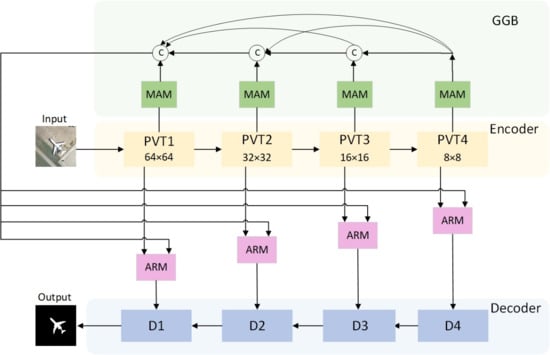
Figure 1 illustrates the comprehensive framework of our proposed GMANet. GMANet comprises four essential components: the PVT-v2 encoder, the GGB, the ARM, and the DD. Notably, the GGB integrates four densely connected MAMs. The overall architectural strategy employs a coarse-to-fine approach. The initial image undergoes processing through the PVT-v2 encoder, generating four feature maps at distinct scales. The MAM combines convolution kernels of different sizes on the same scale to perform multiscale feature aggregation to enhance the perception of scale changes. These multiscale aggregated features are used as the input of the GGB, and the correlation between the features is fully captured by dense connection and learns global context information. Global context information is used to determine the location of salient regions. The ARM then merges the global context information with high-level and low-level features. The resultant amalgamation is subsequently input into the DD, facilitating in-depth analysis and ultimately yielding a refined saliency map. This intricate framework orchestrates a systematic progression from the original image to a nuanced and accurate delineation of salient regions.
To better establish long-range dependencies and image continuity, we use PVT-v2 [43] as the backbone network of the encoder to extract multiscale features. Specifically, we first cut the input image into uniform patches for self-attention, and PVT outputs four groups of feature maps with sizes of 6464, 3232, 1616, and 88, respectively. In order to compute multi-head self-attention more efficiently, PVT uses a sequential reduction method. The input sequence is first reshaped into , and then the MLP is applied to reduce the channel from C r to C. The PVT-v2 encoder generates four blocks at different scales through a series of convolution, down-sampling, self-attention and multi-perceptron. The multiscale feature mapping of the output of these blocks is notated as . These feature maps are then fed into the Global Guidance Branch (GGB) to mine the multiscale contextual information in it. The multiscale features are densely connected and aggregated step by step to learn global context information with global guidance information. Then, the global context information and the multiscale feature maps ( = 1, 2, 3, 4) are fed into the Aggregate Refinement Module (ARM) at the same time, and and the feature maps at all levels are fused respectively to better fuse the global guidance information, high-level semantic information, and local detail information. The fused features are input into the Dense Decoder (DD). The final fine predictive salient map is generated after step-by-step decoding.
3.2. Multiscale Attention Module (MAM)
Optical remote sensing images exhibit distinct characteristics, including extreme scale variation and variable numbers, emphasising the paramount importance of multiscale contextual information in ORSI-SOD. DSS [32] and PoolNet [33] apply fixed-size convolution kernels to extract and aggregate information at different scales. However, the fixed-size convolution kernel can only learn fixed features and capture very limited context information; thus, the current methods do not perform well on images with great scale variation, such as optical remote sensing. We design a Multiscale Attention Module (MAM) to address this challenge. The smaller convolution kernel can capture the detailed features, while the larger convolution kernel can capture a wider range of contextual information. MAM combines convolution kernels of different sizes at the same scale, enhancing the perception of scale changes while reducing information loss. Our approach strategically harnesses both local and global information from features of different resolutions, proving highly effective in determining the precise locations of salient regions.
Recognising the limitations of fixed-size convolutional kernels, which can only learn a predetermined number of features and capture a limited context, we adopt a convolutional strategy involving various kernel sizes applied to the same features. This approach enhances the receptive field, allowing for a more comprehensive understanding of the contextual intricacies. Leveraging the distinctive attributes of high-level features, rich in semantic information, and low-level features, abundant in detailed information, we aggregate these cross-scale features. This aggregation culminates in the creation of a global context feature, amalgamating multiscale contextual and global information. This enriched feature is further integrated with encoder features, providing valuable multi-global contextual information that enhances the precision of salient region localisation. Figure 2 provides a detailed illustration of the MAM, elucidating its intricate mechanisms. We use multiscale feature fusion technology to combine feature maps of different levels, and the combination of max pooling and full connection can help the network focus on the key features of small objects, solving the problem that small objects are easily missed.
Specifically, the input feature is convolved with convolution kernel sizes of 1, 3, 5 and 7, respectively, to obtain four feature maps of different scales, denoted as , , and . This process can be expressed as:
We concatenate the three multiscale features , and , and use 3 × 3 convolution for feature fusion at different scales. The fused feature and feature are multiplied. Common features are extracted by feature intersection, which aims to minimise the interference of noise on salient regions while extracting multiscale features. Then is obtained by adding the fused feature and . This process can be formulated as follows:
The enhanced feature is converted into a channel vector by maximum pooling. We then input this channel vector into the two fully connected layers to obtain the weight of the feature . Finally, we multiply this weight with itself channel by channel, and perform channel-wise weighted highlighting on to obtain the feature . This process can be expressed as follows:
Since feature maps with larger resolutions contain more detailed information, these features do not all belong to the salient object. Therefore, we simultaneously perform max-pooling and 3 × 3 convolution on the feature to transform the input feature into a single channel feature. Finally, we multiply the single channel feature and the channel-weighted feature pixel by pixel to highlight the salient region and suppress the background interference to get the feature . This process can be expressed as:
Finally, using the residual idea, we add the original input feature and feature , and obtain the final output feature after 1 × 1 convolution. This process can be expressed as:
3.3. Global Guided Branch (GGB)
GateNet [31] performs simple global information extraction, which cannot fully use the rich correlation information between features at different scales. In this paper, we design a global guided branch, which densely connects features across scales to better capture the correlation between features at different scales, fully capture the long-range semantic dependencies between all spatial locations, and improve global feature consistency. Figure 1 introduces the GGB, comprising four MAM modules interconnected through dense connections. Each of the four MAM modules individually explores multiscale context information embedded within feature maps of varying resolutions, facilitating the dense aggregation of multiscale features. However, given the semantic disparities among features at different scales, a direct aggregation approach may incur partial information loss and introduce new noise interference. To mitigate these challenges, we implement dense connections to process features. This strategic inclusion emphasises inter-layer feature correlation and learns global context information, denoted as , enriched with global context information. The detailed workings of this GGB are visually depicted in Figure 1.
3.4. Aggregation Refinement Module (ARM)
Effectively combining both local details and global semantic information is pivotal for accurate salient region detection. However, merging these two types of information may not straightforwardly yield optimal results. We introduce a specialised ARM to address this. The ARM strategically employs global information to guide local details and utilises detailed information to enhance global semantics. This reciprocal optimisation process culminates in the aggregation of the two types of information, producing a feature map characterised by precise positioning and rich details. A detailed depiction of the ARM is provided in Figure 3.
The feature maps generated by the PVT-v2 encoder at different scales represent local details, characterised by intricate details but lacking semantic information, thereby introducing noise. The initial enhancement of is achieved through a Transformer (TF) block, yielding the augmented feature . Simultaneously, the global information generated by the GGB possesses semantic richness but lacks intricate details. To address this imbalance, undergoes a channel attention process [44] for channel selection, resulting in the refined feature . Mathematically, this process is expressed as:
Then we multiply and to make the saliency region localisation more accurate, and the resulting feature map is denoted as . At the same time, we optimise global semantic features and local detail features. This process can be expressed as follows:
Finally, the features and are concatenated to obtain the features, which makes the semantic information and detail information better fused, the boundary is clearer, and the noise is reduced. This process can be expressed as follows:
3.5. Dense Decoder (DD)
Traditional decoders [45] typically adopt a cascade structure involving multiple convolutional connections. However, the distinctive feature of ORSI-SOD lies in the substantial scale variations, encompassing scenarios with both small and large objects. In such cases, conventional decoders prove suboptimal. Drawing inspiration from [46], we introduce the DD. Unlike conventional counterparts, dense decoders employ Dense Separable Convolution (DSConv) blocks with a dense structure, as illustrated in Figure 4.
Each dense decoder comprises three DSConvs with dilation rates [47] of 2, 4, and 6, alongside three 1 × 1 convolutions. The utilisation of dilated DSConv facilitates an expanded receptive field while concurrently minimising the parameter count. The 1 × 1 convolution functions to amalgamate densely connected features. The input to the dense decoder is denoted as , and the decoding process unfolds as follows:
where represents a 3 × 3 with an expansion rate of . The DD can obtain features of different scales, better localise the salient regions, and greatly improve accuracy.
In the decoding process, the decoder upsamples the compressed feature map layer by layer, which not only restores the size of the feature map but also reconstructs the features by convolution and gradually restores the image details based on accurate positioning. As shown in Figure 1, the features are decoded by D1–D4 to generate four different saliency maps S1–S4, respectively. The D4 decoder is responsible for recovering the low-level details and texture information of the image. It produces S4 with high resolution to capture subtle variations and details of the input image. The D3 decoder is used to recover the shape of the image. It generates S3, which can show the general outline and structure of salient objects. The D2 decoder is dedicated to recovering the semantic information of the image. It generates S2 with a better understanding of the image’s content. The D1 decoder is responsible for the overall image reconstruction and salient object recovery. The S1 it generates presents the salient object completely and uniquely with high quality. The final output image is simply an upsampling of S1, restoring the image to the same size as the input image. The output image is a saliency map with accurate object localisation, complete structure and clear quality.
3.6. Loss Function
Our approach incorporates deep supervision [48] during the training process. This entails utilising the loss function to supervise feature layers at different levels and scales, ensuring timely parameter adjustments to facilitate comprehensive learning of features across scales and expedite network convergence. Instead of relying on a single loss function, we employ a hybrid loss function that combines Binary Cross-Entropy loss (BCE) and Intersection over Union loss (IoU) [49].
In SOD tasks, the commonly employed BCE loss measures the pixel-wise discrepancy between the predicted mask and the ground truth, emphasising pixel-level loss evaluations. The BCE loss is denoted as follows:
Here represents the ground truth label of the ith pixel, and signifies the predicted salient score. On the other hand, the IoU loss assesses overall architectural similarity, measuring structural congruence rather than individual pixel discrepancies. The IoU loss is expressed as:
In combining both losses, we address both pixel-level differences and overall structural disparities concurrently, enhancing the supervision of the saliency map and aiding in network training. The combined loss function is denoted as:
Here, represents the ground truth, and represent BCE loss and IoU loss, respectively.
In the training phase, as illustrated at the bottom of Figure 1, we employ pixel-level supervision for each decoder block to ensure rapid convergence. Specifically, a convolution is designed after each decoder to generate the saliency map . The combined BCE and IoU losses are iteratively applied to generate the final saliency map.
4. Experimental Results
4.1. Experimental Protocol
4.1.1. Datasets
We conducted comprehensive evaluations on two established public datasets: ORSSD [32] and its extension, EORSSD [34].
ORSSD [32], pioneered by Li et al., marks the inception of public datasets for Remote Sensing Images (RSI). Comprising 800 optical RSI images portraying diverse scenes such as aircraft, islands, lakes, cars, and ships, each image is accompanied by corresponding pixel-level ground truth. For training and testing, we utilise 600 and 200 images, respectively.
EORSSD [34] represents an expanded and more challenging version of ORSSD. It currently stands as the largest public dataset for Optical Remote Sensing Images (ORSI), featuring 2000 images. Here, we allocate 1400 images for training and 600 for testing.
Our network training encompasses the use of EORSSD for model training and subsequent evaluation on both ORSSD and EORSSD datasets.
4.1.2. Network Training Details
The dataset undergoes preprocessing, including augmentation through flipping and rotating, resulting in seven times the original enhanced data. Specifically, 4800 augmented pairs are generated for ORSSD [32], and 11,200 augmented pairs for EORSSD [34]. The training process spans 40 epochs for both datasets, employing the PyTorch [50] 1.11.0 platform with NVIDIA GeForce RTX 3060 Ti for accelerated training. The PVT-v2 serves as the encoder, initialising network parameters, while new layers are initialised using a normal distribution [51]. The learning rate is initialised at 1 × 10⁻⁴, diminishing by a factor of 10 every 30 epochs. The batch size is set at 4 to align with GPU memory constraints, and the Adam optimiser [52] is employed. The code will be available at https://github.com/houjiayue/GMANet (accessed date: 31 January 2024).
4.1.3. Evaluation Metrics
We utilise seven widely accepted metrics in Salient Object Detection (SOD) tasks for comprehensive evaluation: S-measure (, ) [53], maximum, mean, and adaptive F-measure (i.e., , and ) [54], E-measure () [55], Mean Absolute Error (MAE, M), and Precision-Recall (PR) curves.
S-measure assesses region-aware and object-aware structural similarity, measuring the similarity between foreground pixels and ground truth, with larger values indicating better performance.
F-measure strikes a balance between precision and recall, serving as a weighted average of both, with higher values indicating superior performance.
E-measure combines pixel-level local information with image-level global information, with larger values indicating improved performance.
MAE calculates the average of absolute errors between the predicted and true values, with smaller values signifying better pixel-wise accuracy.
Precision-Recall (PR) curves portray the relationship between precision and recall, with thresholds ranging from 0 to 255. A PR curve closer to the top-right corner indicates superior performance.
4.2. Comparison with State-of-the-Arts
4.2.1. Comparison Methods
Our proposed methods were systematically compared against 28 contemporary techniques, categorised into four groups: traditional Natural Scene Image Salient Object Detection (NSI-SOD) methods, CNN-based NSI-SOD methods, traditional Optical Remote Sensing Image Salient Object Detection (ORSI-SOD) methods, and CNN-based ORSI-SOD methods. The breakdown of methods in each category is as follows:
CNN-based NSI-SOD Method (11 methods): DSS [56], RADF [57], R3Net [58], PoolNet [27], EGNet [18], GCPA [59], MINet [60], ITSD [61], GateNet [28], SUCA [62], PA-KRN [63].
CNN-based ORSI-SOD Method (9 methods): LVNet [32], DAFNet [34], MJRBM [36], CSNet [65], SAMNet [17], AccoNet [66], CorrNet [46], MSCNet [67], MCCNet [37].
We did the following to ensure the fairness of the experiment. The same dataset is used: Each method is evaluated on the ORSSD and EORSSD datasets. The same training period and parameters are used: For fair evaluation, we meticulously retrained AccoNet [66], CorrNet [46], MSCNet [67], and MCCNet [37] using the same training parameters, all initialising the learning rate to 1 × 10⁻⁴, scaling it down by a factor of 10 every 30 epochs, and setting the batch size to 4. Ensure that all base networks are trained and tested under the same conditions. The same optimisation strategy is adopted: both use the Adam optimiser [52] to optimise the network. The same performance metrics are used: All methods use a unified performance metric to evaluate the models, which can comprehensively reflect the strengths and weaknesses of different models. Comparison under the same backbone network: DAFNet [34], MJRBM [36], and AccoNet [66] methods have different versions of the backbone network, and we uniformly use the VGG version to ensure the same basic network’s performance.
4.2.2. Quantitative Comparison
Table 1 provides a comprehensive quantitative evaluation, comparing our proposed method with 28 contemporary approaches across the EORSSD and ORSSD datasets. The assessment is based on key metrics, including , and . Notably, the first five indicators reflect a superior performance with larger values, while the last indicator, M, signifies better results with smaller values. This thorough comparison aims to elucidate the efficacy and competitiveness of our proposed method in relation to existing state-of-the-art techniques.
Upon evaluation on the EORSSD dataset, our method achieved a top-ranking position in four metrics, secured the second position in one, and attained the third position in one, emerging as the overall best performer. Notably, among existing NSI-SOD methods, PA-KRN demonstrated superior performance because PA-KRN can better model the location information of the object in the image by introducing a location-aware mechanism. However, our proposed method exhibited significant advantages across all indicators, except for a marginal 0.04% shortfall in . Specifically, our method surpassed PA-KRN by 2.67%, 1.18%, 3.50%, and 0.34% in , respectively, while registering a modest 0.33% decrease in M. This advantage in data is because our method uses multiple convolution kernels of different sizes to perform convolution operations on the feature map, which better fuses the feature information of multiple scales. This multiscale feature fusion helps improve object detection performance and has strong adaptability to objects with extreme scale changes. Additionally, our method outperformed the leading ORSI-SOD method, MCCNet, across all metrics, showcasing substantial improvements, especially with a notable 1.15% enhancement in and a 0.97% reduction in . This benefits from our method’s dense connections in the global guidance branch and decoder, which can better capture the correlation between features at different scales.
On the ORSSD dataset, our method secured the top position in all five metrics, distinguishing itself as the only method with surpassing 0.86, exceeding 0.88, and surpassing 0.97. Compared to the leading PA-KRN method, our approach exhibited significant advantages with higher values of 1.12%, 0.97%, 3.05%, and 0.28% in , respectively. In contrast to eight traditional methods, encompassing both NSI-SOD and ORSI-SOD, as well as 11 CNN-based NSI-SOD methods, our method consistently outperformed the competition. This is because our approach focuses on capturing remote dependencies, overcoming the disadvantage of focusing on local feature learning. At the same time, the coarse-to-fine strategy can add rich details to global information and improve object detection accuracy.
In terms of speed, GMANet is not dominant compared to other salient object detection methods. This is because we extract features using PVT-v2, which consists of multiple transformer blocks and pays more attention to modelling long-range dependencies in the image, which means that it requires self-attention computation at more locations. This causes the model to perform more computational operations on the input image, which slows down inference. Despite its relatively slow speed, GMANet is more accurate in perceptual ability and semantic understanding. Regarding model size, CSNet is the smallest network, but every salient object detection evaluation metric is inferior to our method. GMANet performs better than them in terms of evaluation metrics than methods of similar size. GMANet can be used for image editing and enhancement tasks, such as highlighting important objects or adjusting the focus of an image in some photo processing software.
Furthermore, we include the Precision-Recall (PR) curve in Figure 5, revealing that the PR curve associated with our method resides closer to the top right corner compared to all the methods under comparison. This substantiates the assertion that our proposed method stands out as the most effective performer.
Upon scrutinising the tabulated results, a discernible trend emerges: the CNN-based ORSI-SOD method consistently outperforms its NSI-SOD counterpart. This observation leads to the conclusion that a specialised approach yields superior performance. Thus, it underscores the critical importance of devising methods explicitly tailored for ORSI to attain optimal results. This further fortifies our conviction in the efficacy of specialised methodologies for ORSI diagrams.
4.2.3. Visual Comparison
In Figure 6, we present illustrative examples showcasing the qualitative efficacy of our method. These instances encompass scenarios with multiple tiny objects, irregular geometric structures, objects with shadows, objects against complex backgrounds, objects with low contrast, and objects with interferences. Additionally, we compare the saliency maps generated by our method with those from eight advanced methods. This set includes three CNN-based ORSI-SOD methods (MCCNet, AccoNet, and LVNet), three CNN-based NSI-SOD methods (PA-KRN, GateNet, and MINet), and one traditional ORSI-SOD method (CMC) and a traditional NSI-SOD method (SMD).
- (1)
- Multiple tiny objects. This scenario features a combination of multiple and tiny objects. The distinct shooting distance and angle in ORSI images make small objects significantly smaller than those in NSI, presenting a challenge in detecting all small objects comprehensively. The CNN-based methods in the first row often miss or misdetect salient objects, and traditional methods struggle to adapt to ORSI. In contrast, our method comprehensively detects all objects in scenes with multiple salient objects. This is due to the multiscale feature fusion technique that we use in MAM to combine features from different levels. The shallow detail and deep semantic information are fused to better deal with objects of different sizes. Second, we introduce an attention mechanism to focus on the key features of small objects. In the deep layer of the network, we use upsampling to enlarge the feature map and fuse it with the shallow features so as to recover the lost detailed information. In this way, our network can guarantee the effectiveness and accuracy of small object processing.
- (2)
- Irregular geometry structure. These structures exhibit intricate and irregular topologies, making accurate edge delineation challenging. They appear at various positions and sizes in the image. While AccoNet, LVNet, and MINet can only detect a portion of the river, other methods encounter difficulties, such as introducing noise and unclear edges. Our method, however, accurately detects rivers with complete structures and clear boundaries, notably capturing the lower-left region of the island. We extracted the global context information to improve the clarity of the boundary, which is beneficial to identify the irregular geometry structure of the image.
- (3)
- Objects with shadows. Shadows, often misdetected as salient objects, can create inaccurate detection results. Other methods may miss one or two circles, and GateNet incorrectly highlights shadows. In contrast, our method adeptly detects objects without redundant shadow regions.
- (4)
- Objects with complex backgrounds. The multiscale attention module we designed uses the attention mechanism to highlight salient objects while suppressing background information effectively. Enhance the ability to recognise objects with complex backgrounds. Our results exhibit superior noise reduction, effectively shielding background interference and precisely capturing salient objects.
- (5)
- Objects with low contrast. When salient objects closely resemble the background, many existing methods struggle to highlight them accurately. The lines detected using the three NSI-SOD methods appear fuzzy, and MCCNet fails to detect lines altogether. Conversely, our method yields clear detections, particularly demarcating the accurate boundaries of small islands.
- (6)
- Objects with interferences. Some non-salient objects may interfere with detection, leading to incorrect highlights. Our method can distinguish the interfering objects by modelling the context information around the target, including object shape, texture, etc. In addition, we use the attention mechanism to weight the feature selection and weighting, which also makes the model pay more attention to the features that are helpful to the target and reduce the impact of interfering objects. Our method excels in distinguishing and accurately highlighting salient objects in the presence of potential interferences.
Our method adeptly leverages contextual information, global semantic details, and intricate image features. It effectively addresses challenges related to scale, location, number, and shape variations in ORSI, demonstrating robustness and accuracy in highlighting salient objects across diverse scenarios.
Inspired by the visualisation results, we also ponder some specific applications of GMANet in specific domains. In terms of urban planning, our network can be used for urban development, infrastructure layout, and land use planning to help planners make rational decisions from a clear view of the urban layout. In terms of environmental monitoring, relevant personnel can monitor forest cover change, water pollution, land degradation, etc., based on the saliency map provided by the network, which is crucial for environmental protection and sustainable management. In terms of resource exploration, this method supports resource exploration in remote or inaccessible areas, which is conducive to discovering natural resources such as water and minerals. In the future, the network has potential application value in Marine and coastal detection, agricultural monitoring, etc.
4.3. Ablation Experiment
This section presents comprehensive experiments designed to assess the effectiveness of crucial components within our GMANet on both the EORSSD and ORSSD datasets. The experiments focus on the following aspects: (1) the distinct contributions of the ARM and the GGB, (2) the significance of dense links within the GGB branch, (3) the rationale behind the dilation rate design in the MAM, (4) the effectiveness of the Transformer (TF) block and Channel Attention (CA) block within the ARM module, (5) the efficacy of the MAM module. Additionally, (6) we explore the complementarity between Binary Cross-Entropy (BCE) and Intersection over Union (IoU) in the loss function.
In each variant experiment, modifications are made to only one component at a time, and the model is retrained on both datasets, adhering strictly to the parameters and training methods outlined in Section 4.1.
- (1)
- Individual contribution of each module in the network: To assess the distinct contributions of each module, namely the ARM module and GGB, we propose three variants of GMANet in Table 2.
Baseline: The base network comprises only the encoder-decoder, where the encoder is PVT-v2, and the decoder is the dense decoder.
Baseline + ARM: GGB is removed, retaining only the ARM module. Given the absence of GGB, the dual input of the ARM module is modified to a single input—the multiscale feature map output by the encoder. This feature map directly passes through a transformer and a convolution layer with a 3 × 3 convolution kernel.
Baseline + GGB: The ARM module is omitted, and the feature maps generated by GGB are directly connected to the dense decoder.
Baseline + ARM + GGB: This represents the complete network structure, where both the ARM module and GGB are incorporated into the network to form GMANet. Quantitative results are presented in Table 2.
As presented in Table 2, on the EORSSD dataset, the “baseline” achieves 86.08% on , 94.94% on , 91.35% on , and 0.0094 on . Comparatively, the “ARM” module exhibits increases of 0.83%, 0.67%, and 0.60% in these three metrics, respectively, compared to the “baseline.” Similarly, the “GGB” branch demonstrates improvements of 0.22%, 1.33%, and 0.04% over the “baseline” in these corresponding metrics. In the collaborative application of both “ARM” and “GGB,” there are respective increases of 1.37%, 1.29%, and 0.92% compared to the “Baseline,” validating the efficacy of the “ARM” and “GGB” modules and their synergistic impact. The trend observed on the ORSSD dataset aligns consistently with the EORSSD dataset, thus affirming the effectiveness of each proposed module.
- (2)
As indicated in Table 3, on the EORSSD dataset, GGB-1 achieves 86.88% on , 95.87% on , and 90.44% on . In comparison, GGB-2 attains 87.45% in , 96.23% in , and 92.27% in , representing increases of 0.57%, 0.36%, and 0.44%, respectively. Similarly, these three metrics show improvement on the ORSSD dataset, with increases of 1.29%, 0.45%, and 0.59%, respectively. The rationale behind this lies in the notable feature of ORSI, characterised by substantial scale variation. A direct connection may result in inadequate fusion of feature maps across different scales, whereas a dense connection facilitates more effective layer-by-layer fusion of feature maps at varying scales. Therefore, we opt for the GGB-2 structure, demonstrating superior effectiveness as the GGB of the network.
- (3)
- The rationality of expansion rate design in the MAM module: We present two MAM module variants to assess the rationality of dilation rates in dilated convolutions within the MAM module. The first variant features dilation rates of 1, 3, 5, and 7, mirroring the dilation rates employed by our network. The second variant adopts dilation rates of 3, 5, 7, and 9, respectively, while keeping other components unchanged. The quantitative results are presented in Table 4.
As indicated in Table 4, on the EORSSD dataset, the of the method with d = 1,3,5,7 is 0.8745, is 0.9623, and is 0.9227. However, with an increase in dilation rate to d = 3, 5, 7, and 9, these three indices experience a decrease of 0.76%, 0.24%, and 0.33%, respectively. The trend observed in the ORSSD dataset aligns with the pattern identified in the EORSSD dataset. The enlargement of the dilation rate corresponds to a wider receptive field, thereby enhancing the network’s perceptual capabilities. Distinct dilation rates result in varied receptive fields, acquiring multiscale information. However, with a continuous increase in the dilation rate, diminishing returns are noted. This is attributed to the large receptive field causing the network to struggle to accurately capture variable-scale salient objects in optical remote sensing images. Optimal results are achieved with d = 1, 3, 5, and 7 on both the EORSSD and ORSSD datasets, affirming the rationality of our chosen dilation rate.
- (4)
- The efficacy of the Transformer (TF) and Channel Attention (CA) components in the ARM is assessed through ablation experiments, where two ARM variants are presented: (1) “w/o TF,” which excludes transformer blocks, and (2) “w/o CA,” which omits the channel attention module. The complete ARM module, denoted as “w/TF + CA,” is also included for reference. The quantitative results are presented in Table 5.
Upon examination of the ablation experiment results in Table 5, it is evident that the performance experiences degradation in the absence of both TF and CA blocks in the ARM module. Specifically, on the EORSSD dataset, the removal of TF blocks results in a decrease of 0.64% in , 0.24% in , and 0.39% in . Similarly, without CA blocks, these metrics decrease by 0.65%, 0.78%, and 0.52%, respectively. The ORSSD dataset exhibits a consistent trend with the EORSSD dataset. The transformer is adept at capturing remote dependencies, showcasing a robust ability to model relationships across distant regions and adaptively extract global context information. This characteristic is particularly beneficial for images with significant scale variations, such as those encountered in ORSI. On the other hand, channel attention predicts channel importance and assigns varying weights to each channel to accentuate salient regions while disregarding less relevant information. Consequently, channel attention facilitates the redistribution of feature weights, reducing noise. This substantiates the efficacy of TF and CA in the ARM module.
- (5)
- To demonstrate the role of BCE losses and IoU losses in the loss function, we designed three variants: the first is an approach using only BCE loss. The second is an approach using only IoU loss. The third method is the mixed loss method of BCE and IoU, which is the comprehensive loss used in this paper. The quantitative results are shown in Table 6.
Examination of Table 6 reveals that training the GMANet network with either solely BCE loss or IoU loss individually yields decent performance. For BCE loss on the EORSSD dataset, is 0.8448, is 0.8667, and is 0.8849. On the ORSSD dataset, is 0.8721, is 0.9057, and is 0.8555. Meanwhile, IoU loss exhibits superior performance compared to the BCE loss. However, employing both loss functions in tandem during network training results in improved performance. On the EORSSD dataset, increases by 2.97%, increases by 9.56%, and increases by 3.78%. Similarly, on the ORSSD dataset, increases by 3.47%, increases by 6.57%, and increases by 7.13%. BCE loss, offering pixel-wise supervision, measures the loss between the predicted mask and true values at each pixel. In contrast, IoU loss, providing map-level supervision, evaluates structural similarity without concentrating solely on individual pixels. Their combination yields a synergistic effect, with the two losses complementing each other. Therefore, the conclusion is drawn that training the network with the combined BCE and IoU loss functions produces superior results.
- (6)
- To verify the relative contribution of BCE and IoU loss functions, we set 11 variant forms: 0 × BCE + 1 × IoU, 0.1 × BCE + 0.9× IoU, 0.2 × BCE + 0.8 × IoU, 0.3 × BCE + 0.7 × IoU, 0.4 × BCE + 0.6 × IoU, 0.5 × BCE + 0.5 × IoU, 0.6 × BCE + 0.4 × IoU, 0.7 × BCE + 0.3 × IoU, 0.8 × BCE + 0.2 × IoU, 0.9 × BCE + 0.1 × IoU, 1 × BCE + 0 × IoU, where 0.5 × BCE + 0.5 × IoU is the loss function used by our method. The quantitative results are shown in Figure 8.
The results in Figure 8 show that with the increase in BCE ratio, the experimental effect is gradually improved, and the best effect is achieved at 50% BCE + 50% IoU. However, as the IoU ratio continues to increase, the experimental effect gradually decreases. This is because the BCE loss provides pixel-wise supervision, and the IoU loss provides map-level supervision, evaluating the similarity of structures. Both are equally important and setting them in equal proportions will provide full supervision of the images. Therefore, we choose the mixed loss of 50% BCE + 50% IoU as the loss function of this method.
5. Conclusions
In this paper, we combine the three aspects of global context, feature fusion and dense connection, deeply explore the relationship between features, and propose a GMANet network specifically for optical remote sensing images. First, we use the Pyramid Vision Transformer (PVT-V2) encoder to capture remote dependencies and address the limitations of CNN-based models. To adapt to the large-scale variation of ORSI, we propose the MAM module for learning multiscale information. We then propose the Global Guided Branch, which consists of four densely connected MAM modules for learning global context information. We propose the ARM module between the encoder and decoder to fuse global and detailed information better. We also refer to the Dense Decoder to increase the receptive field and obtain accurate localisation information. In particular, we employ the supervision of hybrid loss to improve the network’s performance. A large number of experiments and ablation experiments show that our proposed method has strong superiority among 28 methods and can obtain relatively complete and accurate salient regions. Nevertheless, the proposed method may encounter challenges in accurately detecting images with extremely fine edges, such as aeroplanes. Future work will explore integrating edge detection methods to enhance model accuracy in such scenarios.
Author Contributions
Conceptualisation, J.H.; Formal analysis, J.F. and W.W.; Supervision, L.H.; Writing—original draft, J.H.; Writing—review and editing, L.H., J.F., W.W. and J.L. All authors will be informed about each step of manuscript processing including submission, revision. All authors have read and agreed to the published version of the manuscript.
Funding
This work was supported by the National Natural Science Foundation of China (No. 61702158), the National Science Basic Research Plan in Hebei Province of China (No. F2018205137), Educational Commission of Hebei Province of China (No. ZD2020317), and the Central Guidance on Local Science and Technology Development Fund of Hebei Province (226Z1808G, 236Z0102G), and the Science and technology research Fund of Hebei Normal University (L2024ZD15, L2022B22).
Data Availability Statement
The datasets used in this experiment can be accessed at the following address: EORSSD: https://pan.baidu.com/s/1xBtxveVJ4qXcvjuWcIOWWg. ORSSD: https://pan.baidu.com/s/1dtzmjk5pvtDFHN1OXfKyBQ. password: fh23 (permanent validity).
Conflicts of Interest
The authors declare no conflicts of interest.
References
- Borji, A.; Cheng, M.M.; Jiang, H.; Li, J. Salient object detection: A benchmark. IEEE Trans. Image Process. 2015, 24, 5706–5722. [Google Scholar] [CrossRef] [PubMed]
- Li, G.; Liu, Z.; Shi, R.; Wei, W. Constrained fixation point based segmentation via deep neural network. Neurocomputing 2019, 368, 180–187. [Google Scholar] [CrossRef]
- Fang, Y.; Chen, Z.; Lin, W.; Lin, C.W. Saliency detection in the compressed domain for adaptive image retargeting. IEEE Trans. Image Process. 2012, 21, 3888–3901. [Google Scholar] [CrossRef] [PubMed]
- Wang, Q.; Lin, J.; Yuan, Y. Salient band selection for hyperspectral image classification via manifold ranking. IEEE Trans. Neural Netw. Learn. Syst. 2016, 27, 1279–1289. [Google Scholar] [CrossRef] [PubMed]
- LeCun, Y.; Boser, B.; Denker, J.S.; Henderson, D.; Howard, R.E.; Hubbard, W.; Jackel, L.D. Backpropagation applied to handwritten zip code recognition. Neural Comput. 1989, 1, 541–551. [Google Scholar] [CrossRef]
- Borji, A.; Cheng, M.M.; Hou, Q.; Jiang, H.; Li, J. Salient object detection: A survey. Comput. Vis. Media 2019, 5, 117–150. [Google Scholar] [CrossRef]
- Wang, W.; Lai, Q.; Fu, H.; Shen, J.; Ling, H.; Yang, R. Salient object detection in the deep learning era: An in-depth survey. IEEE Trans. Pattern Anal. Mach. Intell. 2021, 44, 3239–3259. [Google Scholar] [CrossRef]
- Li, G.; Liu, Z.; Ling, H. ICNet: Information conversion network for RGB-D based salient object detection. IEEE Trans. Image Process. 2020, 29, 4873–4884. [Google Scholar] [CrossRef]
- Li, G.; Liu, Z.; Ye, L.; Wang, Y.; Ling, H. Cross-modal weighting network for RGB-D salient object detection. In Proceedings of the European Conference on Computer Vision, Glasgow, UK, 23–28 August 2020; Springer International Publishing: Cham, Switzerland, 2020; pp. 665–681. [Google Scholar]
- Zou, Z.; Shi, Z.; Guo, Y.; Ye, J. Object detection in 20 years: A survey. In Proceedings of the IEEE International Conference on Computer Vision, Paris, France, 2–6 October 2023. [Google Scholar]
- Pimentel, M.A.F.; Clifton, D.A.; Clifton, L.; Tarassenko, L. A review of novelty detection. Signal Process. 2014, 99, 215–249. [Google Scholar] [CrossRef]
- Chandola, V.; Banerjee, A.; Kumar, V. Anomaly detection: A survey. ACM Comput. Surv. 2009, 41, 1–58. [Google Scholar] [CrossRef]
- Madhulatha, T.S. An overview on clustering methods. arXiv 2012, arXiv:1205.1117. [Google Scholar] [CrossRef]
- Li, K.; Wan, G.; Cheng, G.; Meng, L.; Han, J. Object detection in optical remote sensing images: A survey and a new benchmark. ISPRS J. Photogramm. Remote Sens. 2020, 159, 296–307. [Google Scholar] [CrossRef]
- Simonyan, K.; Zisserman, A. Very deep convolutional networks for large-scale image recognition. arXiv 2014, arXiv:1409.1556. [Google Scholar]
- He, K.; Zhang, X.; Ren, S.; Sun, J. Deep residual learning for image recognition. In Proceedings of the IEEE Conference on Computer Vision and Pattern Recognition, Las Vegas, NV, USA, 27–30 June 2016; IEEE: Piscataway, NJ, USA, 2016; pp. 770–778. [Google Scholar]
- Liu, Y.; Zhang, X.Y.; Bian, J.W.; Zhang, L.; Cheng, M.M. SAMNet: Stereoscopically attentive multi-scale network for lightweight salient object detection. IEEE Trans. Image Process. 2021, 30, 3804–3814. [Google Scholar] [CrossRef] [PubMed]
- Zhao, J.X.; Liu, J.J.; Fan, D.P.; Cao, Y.; Yang, J.; Cheng, M.M. EGNet: Edge guidance network for salient object detection. In Proceedings of the IEEE/CVF International Conference on Computer Vision, Seoul, Republic of Korea, 27–28 October 2019; IEEE: Piscataway, NJ, USA, 2019; pp. 8779–8788. [Google Scholar]
- Itti, L.; Koch, C.; Niebur, E. A model of saliency-based visual attention for rapid scene analysis. IEEE Trans. Pattern Anal. Mach. Intell. 1998, 20, 1254–1259. [Google Scholar] [CrossRef]
- Li, C.; Yuan, Y.; Cai, W.; Xia, Y.; Feng, D.D. Robust saliency detection via regularised random walks ranking. In Proceedings of the IEEE Conference on Computer Vision and Pattern Recognition, Boston, MA, USA, 7–12 June 2015; pp. 2710–2717. [Google Scholar]
- Yuan, Y.; Li, C.; Kim, J.; Cai, W.; Feng, D.D. Reversion correction and regularised random walk ranking for saliency detection. IEEE Trans. Image Process. 2017, 27, 1311–1322. [Google Scholar] [CrossRef] [PubMed]
- Kim, J.; Han, D.; Tai, Y.W.; Kim, J. Salient region detection via high-dimensional color transform and local spatial support. IEEE trans. Image Process. 2015, 25, 9–23. [Google Scholar] [CrossRef]
- Zhou, L.; Yang, Z.; Zhou, Z.; Hu, D. Salient region detection using diffusion process on a two-layer sparse graph. IEEE Trans. Image Process. 2017, 26, 5882–5894. [Google Scholar] [CrossRef]
- Peng, H.; Li, B.; Ling, H.; Hu, W.; Xiong, W.; Maybank, S.J. Salient object detection via structured matrix decomposition. IEEE Trans. Pattern Anal. Mach. Intell. 2016, 39, 818–832. [Google Scholar] [CrossRef]
- Zhou, Y.; Huo, S.; Xiang, W.; Hou, C.; Kung, S.Y. Semi-supervised salient object detection using a linear feedback control system model. IEEE Trans. Cybern. 2018, 49, 1173–1185. [Google Scholar] [CrossRef]
- Liang, M.; Hu, X. Feature selection in supervised saliency prediction. IEEE Trans. Cybern. 2014, 45, 914–926. [Google Scholar] [CrossRef]
- Liu, J.J.; Hou, Q.; Cheng, M.M.; Feng, J.; Jiang, J. A simple pooling-based design for real-time salient object detection. In Proceedings of the IEEE Conference on Computer Vision and Pattern Recognition, Long Beach, CA, USA, 15–20 June 2019; IEEE: Piscataway, NJ, USA, 2019; pp. 3917–3926. [Google Scholar]
- Zhao, X.; Pang, Y.; Zhang, L.; Lu, H.; Zhang, L. Suppress and balance: A simple gated network for salient object detection. In Proceedings of the European Conference on Computer Vision, Glasgow, UK, 23–28 August 2020; Springer International Publishing: Cham, Switzerland, 2020; pp. 35–51. [Google Scholar]
- Ma, M.; Xia, C.; Li, J. Pyramidal feature shrinking for salient object detection. In Proceedings of the AAAI Conference on Artificial Intelligence, Virtual, 2–9 February 2021; AAAI Press: Palo Alto, CA, USA, 2021; pp. 2311–2318. [Google Scholar]
- Qin, X.; Zhang, Z.; Huang, C.; Gao, C.; Dehghan, M.; Jagersand, M. Basnet: Boundary-aware salient object detection. In Proceedings of the IEEE/CVF Conference on Computer Vision and Pattern Recognition, Long Beach, CA, USA, 15–20 June 2019; IEEE: Piscataway, NJ, USA, 2019; pp. 7479–7489. [Google Scholar]
- Zhang, L.; Li, A.; Zhang, Z.; Yang, K. Global and local saliency analysis for the extraction of residential areas in high-spatial-resolution remote sensing image. IEEE Trans. Geosci. Remote Sens. 2016, 54, 3750–3763. [Google Scholar] [CrossRef]
- Li, C.; Cong, R.; Hou, J.; Zhang, S.; Qian, Y.; Kwong, S. Nested network with two-stream pyramid for salient object detection in optical remote sensing images. IEEE Trans. Geosci. Remote Sens. 2019, 57, 9156–9166. [Google Scholar] [CrossRef]
- Li, Q.; Mou, L.; Liu, Q.; Wang, Y.; Zhu, X.X. HSF-Net: Multiscale deep feature embedding for ship detection in optical remote sensing imagery. IEEE Trans. Geosci. Remote Sens. 2018, 56, 7147–7161. [Google Scholar] [CrossRef]
- Zhang, Q.; Cong, R.; Li, C.; Cheng, M.M.; Fang, Y.; Cao, X.; Zhao, Y.; Kwong, S. Dense Attention Fluid Network for Salient Object Detection in Optical Remote Sensing Images. IEEE Trans. Image Process. 2020, 30, 1305–1317. [Google Scholar] [CrossRef] [PubMed]
- Li, C.; Cong, R.; Guo, C.; Li, H.; Zhang, C.; Zheng, F.; Zhao, Y. A parallel down-up fusion network for salient object detection in optical remote sensing images. Neurocomputing 2020, 415, 411–420. [Google Scholar] [CrossRef]
- Tu, Z.; Wang, C.; Li, C.; Fan, M.; Zhao, H.; Luo, B. ORSI salient object detection via multiscale joint region and boundary model. IEEE Trans. Geosci. Remote Sens. 2021, 60, 5607913. [Google Scholar] [CrossRef]
- Li, G.; Liu, Z.; Lin, W.; Ling, H. Multi-content complementation network for salient object detection in optical remote sensing images. IEEE Trans. Geosci. Remote Sens. 2021, 60, 5614513. [Google Scholar] [CrossRef]
- Dong, C.; Liu, J.; Xu, F.; Liu, C. Ship Detection from Optical Remote Sensing Images Using Multi-Scale Analysis and Fourier HOG Descriptor. Remote Sens. 2019, 11, 1529. [Google Scholar] [CrossRef]
- Zhang, Q.; Zhang, L.; Shi, W.; Liu, Y. Airport Extraction via Complementary Saliency Analysis and Saliency-Oriented Active Contour Model. IEEE Geosci. Remote Sens. Lett. 2018, 15, 1085–1089. [Google Scholar] [CrossRef]
- Peng, D.; Guan, H.; Zang, Y.; Bruzzone, L. Full-level domain adaptation for building extraction in very-high-resolution optical remote-sensing images. IEEE Trans. Geosci. Remote Sens. 2021, 60, 1–17. [Google Scholar] [CrossRef]
- Liu, Z.; Zhao, D.; Shi, Z.; Jiang, Z. Unsupervised Saliency Model with Color Markov Chain for Oil Tank Detection. Remote Sens. 2019, 11, 1089. [Google Scholar] [CrossRef]
- Jing, M.; Zhao, D.; Zhou, M.; Gao, Y.; Jiang, Z.; Shi, Z. Unsupervised oil tank detection by shape-guide saliency model. IEEE Trans. Geosci. Remote Sens. 2018, 16, 477–481. [Google Scholar] [CrossRef]
- Dong, B.; Wang, W.; Fan, D.P.; Li, J.; Fu, H.; Shao, L. Polyp-pvt: Polyp segmentation with pyramid vision transformers. arXiv 2021, arXiv:2108.06932. [Google Scholar] [CrossRef]
- Hu, J.; Shen, L.; Sun, G. Squeeze-and-excitation networks. In Proceedings of the IEEE Conference on Computer Vision and Pattern Recognition, Salt Lake City, UT, USA, 18–22 June 2018; IEEE: Piscataway, NJ, USA, 2018; pp. 7132–7141. [Google Scholar]
- Badrinarayanan, V.; Kendall, A.; Cipolla, R. Segnet: A deep convolutional encoder-decoder architecture for image segmentation. IEEE Trans. Pattern Anal. Mach. Intell. 2017, 39, 2481–2495. [Google Scholar] [CrossRef]
- Li, G.; Liu, Z.; Bai, Z.; Lin, W.; Ling, H. Lightweight Salient Object Detection in Optical Remote Sensing Images via Feature Correlation. IEEE Trans. Geosci. Remote Sens. 2022, 60, 5617712. [Google Scholar] [CrossRef]
- Yu, F.; Koltun, V. Multi-scale context aggregation by dilated convolutions. arXiv 2015, arXiv:1511.07122. [Google Scholar]
- Xie, S.; Tu, Z. Holistically-Nested Edge Detection. arXiv 2015, arXiv:1504.06375. [Google Scholar]
- Li, G.; Liu, Z.; Chen, M.; Bai, Z.; Lin, W.; Ling, H. Hierarchical alternate interaction network for RGB-D salient object detection. IEEE Trans. Image Process. 2021, 30, 3528–3542. [Google Scholar] [CrossRef] [PubMed]
- Paszke, A.; Gross, S.; Massa, F.; Lerer, A.; Bradbury, J.; Chanan, G.; Killeen, T.; Lin, Z.; Gimelsshein, N.; Antiga, L.; et al. Pytorch: An imperative style, high-performance deep learning library. Adv. Neural Inf. Process. Syst. 2019, 32. [Google Scholar]
- He, K.; Zhang, X.; Ren, S.; Sun, J. Delving deep into rectifiers: Surpassing human-level performance on ImageNet classification. In Proceedings of the IEEE International Conference on Computer Vision (ICCV), Santiago, Chile, 7–13 December 2015; pp. 1026–1034. [Google Scholar]
- Kingma, D.P.; Ba, J. Adam: A method for stochastic optimization. arXiv 2014, arXiv:1412.6980. [Google Scholar]
- Fan, D.P.; Cheng, M.M.; Liu, Y.; Li, T.; Borji, A. Structure-measure: A new way to evaluate foreground maps. In Proceedings of the IEEE/CVF International Conference on Computer Vision, Venice, Italy, 22–29 October 2017; IEEE: Piscataway, NJ, USA, 2017; pp. 4548–4557. [Google Scholar]
- Achanta, R.; Hemami, S.; Estrada, F.; Susstrunk, S. Frequency-tuned salient region detection. In Proceedings of the 2009 IEEE Conference on Computer Vision and Pattern Recognition, Miami, FL, USA, 20–25 June 2009; pp. 1597–1604. [Google Scholar]
- Fan, D.P.; Gong, C.; Cao, Y.; Ren, B.; Cheng, M.M.; Borji, A. Enhanced-alignment measure for binary foreground map evaluation. In Proceedings of the 27th International Joint Conference on Artifificial Intelligence, Stockholm, Sweden, 13–19 July 2018; AAAI Press: Menlo Park, CA, USA, 2018; pp. 698–704. [Google Scholar]
- Hou, Q.; Cheng, M.; Hu, X.; Borji, A.; Tu, Z.; Torr, P. Deeply Supervised Salient Object Detection with Short Connections. IEEE Trans. Pattern Anal. Mach. Intell. 2019, 41, 815. [Google Scholar] [CrossRef]
- Hu, X.; Zhu, L.; Qin, J.; Fu, C.W.; Heng, P.A. Recurrently aggregating deep features for salient object detection. In Proceedings of the Thirty-Second AAAI Conference on Artifificial Intelligence (AAAI), New Orleans, LA, USA, 2–7 February 2018. [Google Scholar]
- Deng, Z.; Hu, X.; Zhu, L.; Xu, X.; Qin, J.; Han, G.; Heng, P.A. R3net: Recurrent residual refifinement network for saliency detection. In Proceedings of the 27th International Joint Conference on Artifificial Intelligence, Stockholm, Sweden, 13–19 July 2018; AAAI Press: Menlo Park, CA, USA, 2018; pp. 684–690. [Google Scholar]
- Chen, Z.; Xu, Q.; Cong, R.; Huang, Q. Global Context-Aware Progressive Aggregation Network for Salient Object Detection. In Proceedings of the AAAI Conference on Artifificial Intelligence, New York, NY, USA, 7–12 February 2020; AAAI Press: Menlo Park, CA, USA, 2020; pp. 10599–10606. [Google Scholar]
- Pang, Y.; Zhao, X.; Zhang, L.; Lu, H. Multi-Scale Interactive Network for Salient Object Detection. In Proceedings of the IEEE/CVF Conference on Computer Vision and Pattern Recognition (CVPR), Seattle, WA, USA, 14–19 June 2020; pp. 9413–9422. [Google Scholar]
- Zhou, H.; Xie, X.; Lai, J.; Chen, Z.; Yang, L. Interactive two-stream decoder for accurate and fast saliency detection. In Proceedings of the IEEE Conference on Computer Vision and Pattern Recognition (CVPR), Seattle, WA, USA, 13–19 June 2020; pp. 9141–9150. [Google Scholar]
- Li, J.; Pan, Z.; Liu, Q.; Wang, Z. Stacked U-shape network with channel-wise attention for salient object detection. IEEE Trans. Multimed. 2020, 23, 1397–1409. [Google Scholar] [CrossRef]
- Xu, B.; Liang, H.; Liang, R.; Chen, P. Locate globally, segment locally: A progressive architecture with knowledge review network for salient object detection. Proc. AAAI Conf. Artif. Intell. 2021, 35, 3004–3012. [Google Scholar] [CrossRef]
- Zhang, L.; Liu, Y.; Zhang, J. Saliency detection based on self-adaptive multiple feature fusion for remote sensing images. Int. J. Remote Sens. 2019, 40, 8270–8297. [Google Scholar] [CrossRef]
- Gao, S.-H.; Tan, Y.-Q.; Cheng, M.-M.; Lu, C.; Chen, Y.; Yan, S. Highly efficient salient object detection with 100k parameters. In Proceedings of the European Conference on Computer Vision, Glasgow, UK, 23–28 August 2020; pp. 702–721. [Google Scholar]
- Li, G.; Liu, Z.; Zeng, D.; Lin, W.; Ling, H. Adjacent context coordination network for salient object detection in optical remote sensing images. IEEE Trans. Cybern. 2022, 53, 526–538. [Google Scholar] [CrossRef] [PubMed]
- Lin, Y.; Sun, H.; Liu, N.; Bian, Y.; Cen, J.; Zhou, H. A lightweight multi-scale context network for salient object detection in optical remote sensing images. In Proceedings of the 2022 26th International Conference on Pattern Recognition (ICPR), Montreal, QC, Canada, 21–25 August 2022; pp. 238–244. [Google Scholar]
Figure 1.
The overall framework of the proposed Global and Multiscale Aggregate Network for Saliency Object Detection in Optical Remote Sensing Images (GMANet). GMANet consists of four main parts: the PVT-v2 encoder, the global guide branch, the Aggregate Refinement Module (ARM), and the dense decoder (DD), where the global guide branch consists of four densely connected multiscale attention modules (MAM). First, four feature maps of different levels are generated by the encoder PVT-v2, which are fed into the Global Guidance Branch (GGB) to learn global context information. The global context information and high-level and low-level features are fused through the Aggregate Refinement Module (ARM) and then input into the Dense Decoder (DD) for further analysis. Notably, in the training phase, we adopt the deep supervision strategy and attach supervision to each decoder block. GT denotes ground truth.

Figure 2.
Illustration of Multiscale Attention Module (MAM).

Figure 3.
Illustration of Aggregation Refinement Module (ARM).

Figure 4.
Illustration of Dense Decoder (DD). Blue represents DSConv with different dilation rates, and yellow represents 1 × 1 convolution.
Figure 4.
Illustration of Dense Decoder (DD). Blue represents DSConv with different dilation rates, and yellow represents 1 × 1 convolution.

Figure 5.
Quantitative comparison of the PR curves of SOD methods on EORSSD and ORSSD datasets.

Figure 6.
Visual comparisons with eight representative state-of-the-art methods. Please zoom in for the best view.
Figure 6.
Visual comparisons with eight representative state-of-the-art methods. Please zoom in for the best view.

Figure 7.
GGB Variant. (a) Consists of four MAM modules directly spliced, and (b) consists of four MAM modules densely connected.
Figure 7.
GGB Variant. (a) Consists of four MAM modules directly spliced, and (b) consists of four MAM modules densely connected.

Figure 8.
Ablation studies to evaluate the contribution of the BCE and IoU in loss functions. The best result for each column is in bold.
Figure 8.
Ablation studies to evaluate the contribution of the BCE and IoU in loss functions. The best result for each column is in bold.


Table 1.
Quantitative results on two datasets, EORSSD and ORSSD. At present, there are 28 methods studied, including five traditional salient object detection in natural scene images (NSI-SOD) methods, 11 CNN-based NSI-SOD methods, three traditional salient object detection in optical remote sensing images (ORSI-SOD) methods, and 9 CNN-based ORSI-SOD methods. / Indicates that the larger or smaller the score, the better. The top three results are highlighted in red, blue, and green.
| Methods | Type | Speed | EORSSD [34] | ORSSD [32] | |||||||||||
|---|---|---|---|---|---|---|---|---|---|---|---|---|---|---|---|
| RRWR [20] | T.N. | 0.3 | - | 0.5997 | 0.4496 | 0.2906 | 0.3347 | 0.5696 | 0.1677 | 0.6837 | 0.5950 | 0.4254 | 0.4874 | 0.7034 | 0.1323 |
| HDCT [22] | T.N. | 7 | - | 0.5976 | 0.5992 | 0.1891 | 0.2663 | 0.5197 | 0.1087 | 0.6196 | 0.5776 | 0.2617 | 0.3720 | 0.6289 | 0.1309 |
| DSG [23] | T.N. | 0.6 | - | 0.7196 | 0.6630 | 0.4774 | 0.5659 | 0.7573 | 0.1041 | 0.7196 | 0.6630 | 0.4774 | 0.5659 | 0.7573 | 0.1041 |
| SMD [24] | T.N. | - | - | 0.7112 | 0.6469 | 0.4297 | 0.4094 | 0.6428 | 0.0770 | 0.7645 | 0.7075 | 0.5277 | 0.5567 | 0.7680 | 0.0715 |
| RCRR [21] | T.N. | 0.3 | - | 0.6013 | 0.4495 | 0.2907 | 0.3349 | 0.5646 | 0.1644 | 0.6851 | 0.5945 | 0.4255 | 0.4876 | 0.6959 | 0.1276 |
| DSS [56] | C.N. | 8 | 62.23 | 0.7874 | 0.7159 | 0.5393 | 0.4613 | 0.6948 | 0.0186 | 0.8260 | 0.7838 | 0.6536 | 0.6203 | 0.8119 | 0.0363 |
| RADF [57] | C.N. | 7 | 62.54 | 0.8189 | 0.7811 | 0.6296 | 0.4954 | 0.7281 | 0.0168 | 0.8258 | 0.7876 | 0.6256 | 0.5726 | 0.7709 | 0.0382 |
| R3Net [58] | C.N. | 2 | 56.16 | 0.8192 | 0.7710 | 0.5742 | 0.4181 | 0.6477 | 0.0171 | 0.8142 | 0.7824 | 0.7060 | 0.7377 | 0.8721 | 0.0404 |
| PoolNet [27] | C.N. | 25 | 53.63 | 0.8218 | 0.7811 | 0.5778 | 0.4629 | 0.6864 | 0.0210 | 0.8400 | 0.7904 | 0.6641 | 0.6162 | 0.8157 | 0.0358 |
| EGNet [18] | C.N. | 9 | 108.07 | 0.8602 | 0.8059 | 0.6743 | 0.5381 | 0.7578 | 0.0110 | 0.8718 | 0.8431 | 0.7253 | 0.6448 | 0.8276 | 0.0216 |
| GCPA [59] | C.N. | 23 | 67.06 | 0.8870 | 0.8517 | 0.7808 | 0.6724 | 0.8652 | 0.0102 | 0.9023 | 0.8836 | 0.8292 | 0.7853 | 0.9231 | 0.0168 |
| MINet [60] | C.N. | 12 | 47.56 | 0.9040 | 0.8583 | 0.8133 | 0.7707 | 0.9010 | 0.0090 | 0.9038 | 0.8924 | 0.8438 | 0.8242 | 0.9301 | 0.0142 |
| ITSD [61] | C.N. | 16 | 17.08 | 0.9051 | 0.8690 | 0.8114 | 0.7423 | 0.8999 | 0.0108 | 0.9048 | 0.8847 | 0.8376 | 0.8059 | 0.9263 | 0.0166 |
| GateNet [28] | C.N. | 25 | 100.02 | 0.9114 | 0.8731 | 0.8128 | 0.7123 | 0.8755 | 0.0097 | 0.9184 | 0.8967 | 0.8562 | 0.8220 | 0.9307 | 0.0135 |
| SUCA [62] | C.N. | 24 | 117.71 | 0.8988 | 0.8430 | 0.7851 | 0.7274 | 0.8801 | 0.0097 | 0.8988 | 0.8605 | 0.8108 | 0.7745 | 0.9093 | 0.0143 |
| PA-KRN [63] | C.N. | 16 | 141.06 | 0.9193 | 0.8750 | 0.8392 | 0.7995 | 0.9273 | 0.0105 | 0.9240 | 0.8957 | 0.8677 | 0.8546 | 0.9409 | 0.0138 |
| VOS [39] | T.O. | - | - | 0.5083 | 0.3338 | 0.1158 | 0.1843 | 0.4772 | 0.2159 | 0.5367 | 0.3875 | 0.1831 | 0.2633 | 0.5798 | 0.2227 |
| SMFF [64] | T.O. | - | - | 0.5405 | 0.5738 | 0.1012 | 0.2090 | 0.5020 | 0.1434 | 0.5310 | 0.4865 | 0.1383 | 0.2493 | 0.5674 | 0.1854 |
| CMC [41] | T.O. | - | - | 0.5800 | 0.3663 | 0.2025 | 0.2010 | 0.4891 | 0.1057 | 0.6033 | 0.4213 | 0.2904 | 0.3107 | 0.5989 | 0.1267 |
| LVNet [32] | C.O. | 1.4 | - | 0.8645 | 0.8052 | 0.7021 | 0.6308 | 0.8478 | 0.0145 | 0.8813 | 0.8414 | 0.7744 | 0.7500 | 0.9225 | 0.0207 |
| DAFNet [34] | C.O. | 26 | 29.35 | 0.9167 | 0.8688 | 0.7832 | 0.6435 | 0.8155 | 0.0062 | 0.9187 | 0.9027 | 0.8434 | 0.7869 | 0.9189 | 0.0115 |
| MJRBM [36] | C.O. | 32 | 43.54 | 0.9197 | 0.8765 | 0.8135 | 0.7071 | 0.8901 | 0.0099 | 0.9202 | 0.8932 | 0.8432 | 0.8015 | 0.9331 | 0.0163 |
| CSNet [65] | C.O. | 38 | 0.14 | 0.8229 | 0.8486 | 0.5757 | 0.6321 | 0.8293 | 0.0170 | 0.8889 | 0.8920 | 0.7175 | 0.7614 | 0.9070 | 0.0186 |
| SAMNet [17] | C.O. | 44 | 1.33 | 0.8621 | 0.8075 | 0.7010 | 0.6127 | 0.8114 | 0.0134 | 0.8762 | 0.8331 | 0.7294 | 0.6837 | 0.8549 | 0.0219 |
| AccoNet [66] | C.O. | 10.14 | 80.05 | 0.9095 | 0.8638 | 0.8235 | 0.8053 | 0.9450 | 0.0114 | 0.8975 | 0.8656 | 0.8219 | 0.8227 | 0.9415 | 0.0210 |
| CorrNet [46] | C.O. | 100 | 4.09 | 0.8955 | 0.8423 | 0.8043 | 0.7842 | 0.9294 | 0.0131 | 0.8825 | 0.8547 | 0.8054 | 0.8068 | 0.9338 | 0.0238 |
| MSCNet [67] | C.O. | - | - | 0.9010 | 0.8555 | 0.7712 | 0.7448 | 0.9256 | 0.0118 | 0.9198 | 0.8975 | 0.8277 | 0.8355 | 0.9583 | 0.0174 |
| MCCNet [37] | C.O. | 95 | 67.65 | 0.9152 | 0.8714 | 0.8395 | 0.8256 | 0.9527 | 0.0109 | 0.9163 | 0.8836 | 0.8529 | 0.8490 | 0.9551 | 0.0155 |
| Ours | C.O. | 15 | 64.37 | 0.9227 | 0.8746 | 0.8510 | 0.8262 | 0.9623 | 0.0072 | 0.9268 | 0.9069 | 0.8815 | 0.8643 | 0.9714 | 0.0184 |
T.N.: Traditional NSI-SOD method, C.N.:CNN-based NSI-SOD method, T.O.: Traditional ORSI-SOD method, C.O.: CNN-based ORSI-SOD method.
Table 2.
Ablation analysis measuring the overall contribution of ARM and GGB in GMANet. The baseline is the encoder-decoder network. The best result for each column is in bold.
Table 2.
Ablation analysis measuring the overall contribution of ARM and GGB in GMANet. The baseline is the encoder-decoder network. The best result for each column is in bold.
| No. | Baesline | ARM | GGB | EORSSD [34] | ORSSD [32] | ||||||
|---|---|---|---|---|---|---|---|---|---|---|---|
| 1 | ✓ | 0.8608 | 0.9494 | 0.9135 | 0.0094 | 0.8979 | 0.9606 | 0.9088 | 0.0194 | ||
| 2 | ✓ | ✓ | 0.8691 | 0.9561 | 0.9195 | 0.0079 | 0.8999 | 0.9647 | 0.9104 | 0.0152 | |
| 3 | ✓ | ✓ | 0.8630 | 0.9607 | 0.9139 | 0.0091 | 0.9007 | 0.9654 | 0.9174 | 0.0185 | |
| 4 | ✓ | ✓ | ✓ | 0.8745 | 0.9623 | 0.9227 | 0.0072 | 0.9068 | 0.9714 | 0.9268 | 0.0184 |
Table 3.
Ablation experiments for two classes of GGB variants in the GMANet. The best result for each column is in bold.
Table 3.
Ablation experiments for two classes of GGB variants in the GMANet. The best result for each column is in bold.
| Models | EORSSD [34] | ORSSD [32] | ||||
|---|---|---|---|---|---|---|
| GGB-1 | 0.8688 | 0.9587 | 0.9183 | 0.8939 | 0.9669 | 0.9209 |
| GGB-2(our) | 0.8745 | 0.9623 | 0.9227 | 0.9068 | 0.9714 | 0.9268 |
Table 4.
Rationality of expansion rate design in the GMANet. The best result for each column is in bold.
Table 4.
Rationality of expansion rate design in the GMANet. The best result for each column is in bold.
| Models | EORSSD [34] | ORSSD [32] | ||||
|---|---|---|---|---|---|---|
| d = 1,3,5,7 (our) | 0.8745 | 0.9623 | 0.9227 | 0.9068 | 0.9714 | 0.9268 |
| d = 3,5,7,9 | 0.8669 | 0.9599 | 0.9194 | 0.9049 | 0.9672 | 0.9144 |
Table 5.
Effectiveness of TF and CA in the ARM module. The best result for each column is in bold.
| Models | EORSSD [34] | ORSSD [32] | ||||
|---|---|---|---|---|---|---|
| w/o TF | 0.8681 | 0.9599 | 0.9188 | 0.9033 | 0.9612 | 0.9298 |
| w/o CA | 0.8680 | 0.9545 | 0.9175 | 0.8965 | 0.9567 | 0.9162 |
| w/TF + CA(our) | 0.8745 | 0.9623 | 0.9227 | 0.9068 | 0.9714 | 0.9268 |
w/o tf: ARM without TF blocks. w/o ca: ARM without CA blocks. w/tf + ca: ARM for both the TF and CA blocks.
Table 6.
Ablation studies to evaluate the complementarity of the BCE and IoU in loss functions. The best result for each column is in bold.
Disclaimer/Publisher’s Note: The statements, opinions and data contained in all publications are solely those of the individual author(s) and contributor(s) and not of MDPI and/or the editor(s). MDPI and/or the editor(s) disclaim responsibility for any injury to people or property resulting from any ideas, methods, instructions or products referred to in the content. |
© 2024 by the authors. Licensee MDPI, Basel, Switzerland. This article is an open access article distributed under the terms and conditions of the Creative Commons Attribution (CC BY) license (https://creativecommons.org/licenses/by/4.0/).
Share and Cite
MDPI and ACS Style
Huo, L.; Hou, J.; Feng, J.; Wang, W.; Liu, J. Global and Multiscale Aggregate Network for Saliency Object Detection in Optical Remote Sensing Images. Remote Sens. 2024, 16, 624. https://0-doi-org.brum.beds.ac.uk/10.3390/rs16040624
AMA Style
Huo L, Hou J, Feng J, Wang W, Liu J. Global and Multiscale Aggregate Network for Saliency Object Detection in Optical Remote Sensing Images. Remote Sensing. 2024; 16(4):624. https://0-doi-org.brum.beds.ac.uk/10.3390/rs16040624
Chicago/Turabian StyleHuo, Lina, Jiayue Hou, Jie Feng, Wei Wang, and Jinsheng Liu. 2024. "Global and Multiscale Aggregate Network for Saliency Object Detection in Optical Remote Sensing Images" Remote Sensing 16, no. 4: 624. https://0-doi-org.brum.beds.ac.uk/10.3390/rs16040624
Note that from the first issue of 2016, this journal uses article numbers instead of page numbers. See further details here.