Spatiotemporal Protein Variations Based on VIIRS-Derived Regional Protein Algorithm in the Northern East China Sea

Abstract

Over the past two decades, the environmental characteristics of the northern East China Sea (NECS) that make it a crucial spawning ground for commercially significant species have faced substantial impacts due to climate change. Protein (PRT) within phytoplankton, serving as a nitrogen-rich food for organisms of higher trophic levels, is a sensitive indicator to environmental shifts. This study aims to develop a regional PRT algorithm to characterize spatial and temporal variations in the NECS from 2012 to 2022. Employing switching chlorophyll-a and particulate organic nitrogen algorithms, the developed regional PRT algorithm demonstrates enhanced accuracy. Satellite-estimated PRT concentrations, utilizing data from the Visible Infrared Imaging Radiometer Suite (VIIRS), generally align with the 1:1 line when compared to in situ data. Seasonal patterns and spatial distributions of PRT in both the western and eastern parts of the NECS from 2012 to 2022 were discerned, revealing notable differences in the spatial distribution and major controlling factors between these two areas. In conclusion, the regional PRT algorithm significantly improves estimation precision, advancing our understanding of PRT dynamics in the NECS concerning PRT concentration and environmental changes. This research underscores the importance of tailored algorithms in elucidating the intricate relationships between environmental variables and PRT variations in the NECS.

1. Introduction

The northern East China Sea (NECS), located in northwestern Pacific Ocean, stands as one of the world’s largest marginal seas, distinguished by its intricate system of dynamic currents, including the Tsushima Warm Current, Taiwan Warm Current, Yellow Sea Coastal Current, and Changjiang diluted water [1,2]. This complex environmental condition fosters abundant fishery resources, rendering the NECS a pivotal spawning ground for commercially significant species like anchovies and hairtail, vital to the Korean fishery industry [3].

In the context of phytoplankton research, regional studies play a pivotal role in unraveling the nuanced dynamics of marine ecosystems. The NECS, with its distinctive environmental features and intricate interactions [1,2], presents a compelling case for targeted regional exploration. The NECS’s complex environmental conditions, influenced by both natural processes and anthropogenic factors, necessitate an in-depth investigation to decipher the intricacies of phytoplankton responses to these unique stressors.

One key aspect that distinguishes the NECS from other regions is its susceptibility to the impacts of climate change, which, over the past two decades [4], has resulted in altered oceanic conditions that potentially affect phytoplankton dynamics. Moreover, the NECS’s role as a critical fishery resource underscores the importance of understanding the specific factors influencing phytoplankton as primary producers in this region. Phytoplankton, which demonstrate a heightened sensitivity to environmental changes, play a critical role in the food web and the biogeochemical cycling of aquatic ecosystems [5,6,7,8]. The biochemical composition of phytoplankton, comprising carbohydrates, proteins, and lipids, provides valuable insights into their physiological and qualitative states [7,9]. Among these components, proteins (PRT) play a crucial role in biological processes such as enzyme catalysis and growth [10], offering nitrogen-rich sustenance for organisms of higher trophic levels compared to carbohydrates and lipids [11,12,13]. Geider et al. [14] highlighted the pivotal connection between PRT and fundamental functions such as biosynthesis and cell division, distinguishing them from other components associated with energy and carbon reservoirs. The synthesis of PRT in actively growing phytoplankton, predominantly regulated by nitrogen availability, serves as a pivotal physiological process [15,16]. The discernible higher incorporation of carbon into PRT serves as a robust indicator of the health and growth status of phytoplankton under conditions of light intensity and/or nutrient concentration, especially with regard to nitrogen limitations [17,18,19]. Understanding these associations provides valuable insights into the intricate dynamics between phytoplankton growth, environmental factors, and the vital role of proteins in sustaining optimal physiological conditions [5,6,7,8,9]. Despite the NECS’s ecological significance [3], studies on PRT within this region remain limited. Notably, the estimation of PRT concentration in the NECS using satellite approaches remains underexplored.

The distinct hydrodynamic and ecological characteristics of the NECS necessitate a specialized regional algorithm tailored to its unique conditions. While regional algorithms have proven successful in various marine environments, the NECS’s specific features, including its dynamic currents and the intricate interplay of environmental factors, warrant a dedicated approach [1,2]. This study seeks to contribute not only to the broader understanding of phytoplankton dynamics but also to fill a critical gap in the knowledge of the NECS, emphasizing the need for region-specific investigations to comprehensively grasp the implications of environmental changes on this pivotal marine ecosystem.

Therefore, this study aims to bridge this gap by developing a new regional algorithm for PRT concentration in phytoplankton, enabling the identification of long-term and large-scale spatial variations in PRT concentration. The primary objectives of this study encompass: (1) the development of a robust regional algorithm for PRT concentration in phytoplankton based on in situ data, (2) the identification of principal controlling factors influencing PRT concentration, and (3) the comprehensive characterization of spatial and temporal variations in PRT concentration using ocean color data in the NECS over an observation period from 2012 to 2022. Through this study, we aim to contribute important insights into the intricate dynamics of phytoplankton PRT concentrations in the NECS, providing their ecological implications and the broader impacts of climate change on this vital marine ecosystem.

2. Materials and Methods

2.1. In Situ Data Collection

Field measurements of total chlorophyll-a (Chla), particulate organic nitrogen (PON), and protein (PRT) concentrations were collected through various research cruises conducted in the northern East China Sea (NECS) from 2018 to 2022. The sampling stations are plotted in Figure 1.

Water samples for the analysis of Chla, PON, and PRT concentrations were obtained from the surface using a CTD/rosette sampler equipped with Niskin bottles. The water samples (300–500 mL) designated for Chla and PON concentrations of phytoplankton underwent filtration through precombusted Whatman GF/F filters (diameter = 25 mm). For PRT analysis, a 1 L volume of water sample was filtered through pre-combusted Whatman GF/F filters (diameter = 47 mm). All filters were promptly preserved at −80 °C for subsequent analysis.

In a home laboratory, Chla concentrations were determined using a Turner De-signs model 10-AU fluorometer following the extraction process with 90% acetone for 24 h at 4 °C in darkness, following the method of Parsons et al. [20]. The PON concentrations were analyzed at the Alaska Stable Isotope Facility, USA. For PRT extractions, we conducted colorimetric peptide-detecting assays, adapting a modified procedure based on Lowry et al. [21]. Specifically, GF/F filters containing filtered samples were fragmented into small segments and transferred to a 12 mL centrifuge tube containing 1 mL of deionized water. Ultrasonification was then performed for PRT extraction for a duration of 20 min. Subsequently, 5 mL of an alkaline copper solution was introduced into the tube, and the solution was thoroughly mixed using a vortex mixer (MaXshakeTM VM30, Daihan Scientific Co., Ltd., Wonju City, Gangwon-do, Republic of Korea), then allowed to stand for 10 min at room temperature. Following this, the sample tubes were supplemented with 0.5 mL of diluted Folin-Ciocalteu phenol reagent (1:1, v/v) and subjected to vortex mixing. After standing at room temperature for 1 h and 30 min, the solutions underwent centrifugation at 3000 rpm for 10 min. The absorbency of the resulting supernatant was measured at 750 nm using a UV spectrophotometer (Labomed Inc., Culver City, CA, USA). Bovine Serum Albumin (2 mg mL⁻¹, Sigma-Aldrich of Korea, Seoul City, Republic of Korea) served as the standards for quantifying PRT concentration.

2.2. Development of the Regional PRT Algorithm

The regional PRT algorithm in the NECS was developed using an empirical approach. A total of 124 in situ data points were utilized in the development of this algorithm. Through multiple linear regression analysis, factors influencing PRT were identified. In situ PRT served as the dependent variable, while independent variables included Chla, PON, Sea Surface Temperature (SST), Sea Surface Salinity (SSS), and Sea Surface Nitrate (SSN). The evaluation for multicollinearity during the multiple linear regression analysis was carried out using the variance inflation factor (VIF) [22,23,24]. A VIF value exceeding 1 suggests a moderate correlation, while a range between 5 and 10 indicates a strong correlation that may be problematic. When the VIF surpasses 10, it signifies potential errors in the regression analysis due to multicollinearity.

2.3. Satellite Ocean Color Data

Satellite-derived Ocean color data were sourced from the Visual Infrared Imaging Radiometer Suite (VIIRS) on the Suomi National Polar-orbiting Partnership (SNPP) satellite. Daily level-3 Remote Sensing Reflectance (Rrs) datasets at specific wavelengths of 410 nm, 443 nm, 486 nm, 551 nm, and 671 nm, encompassing the NECS, were obtained for the period from January 2012 to December 2022 with 4 km of spatial resolution. Additionally, daily level-3 total absorption coefficient at 486 nm (a(486)) datasets were also acquired at the same 4 km of spatial resolution. Bathymetry data with an approximate spatial resolution of 460 m were obtained from the General Bathymetric Chart of the Oceans (GEBCO) to mitigate errors stemming from shallow regions (<20 m) [25,26]. Various environmental parameters were also integrated from different satellites to discern the major controlling factors for PRT (

Table 1. Information from the satellite data: variables, abbreviations, spatial/temporal resolution, and dataset.

Variables	Abbreviation (Unit)	Spatial/Temporal Resolution	Dataset
Photosynthetic available radiation	PAR (Einstein m−2 d−1)	4 km × 4 km, monthly	SNPP-VIIRS
Sea surface temperature	SST (°C)	4 km × 4 km, monthly	SNPP-VIIRS
Suspended particulate matter	SPM (mg L−1)	4 km × 4 km, monthly	Copernicus-Globcolour
Sea surface salinity	SSS (psu)	0.083° × 0.083°, monthly	Copernicus-Global Ocean Physics Reanalysis
Mixed layer depth	MLD (m)	0.083° × 0.083°, monthly
Wind Speed	Wind speed (m s−1)	0.25° × 0.25°, monthly	Cross-Calibrated Multi-Platform

).

2.4. Regional Chla Algorithm for the NECS

Satellite-estimated Chla concentration was derived using 306 in situ data from 2018 to 2022. The Chla retrieval method proposed by Siswanto et al. [27] was measured for the satellite-derived Chla. This method employed a switching approach based on turbidity to differentiate between Case I and Case II waters. Turbidity conditions were indicated by nLw₅₅₁ [28,29]. For Case Ι water (nLw₅₅₁ < 2 m W cm⁻² μm⁻¹ sr⁻¹), the regionally tuned NASA standard OC3 algorithm [30] by Siswanto et al. [27] was used as follows:

$$\mathrm{Chl}a={10}^{(0.366-3.067 \mathrm{R} + 1.930 {\mathrm{R}}^2 + 0.649 {\mathrm{R}}^3-1.532 {\mathrm{R}}^4)}$$

(1)

$$\mathrm{R}={\mathrm{Log}}_{10}\left(\max \left[\frac{{\mathrm{Rrs}}_{443}}{{\mathrm{Rrs}}_{551}}, \frac{{\mathrm{Rrs}}_{486}}{{\mathrm{Rrs}}_{551}}\right]\right)$$

(2)

For the Case II water (nLw₅₅₁ ≥ 2 m W cm⁻² μm⁻¹ sr⁻¹), a modified Tassan [31]-like algorithm, T_chl_T_chl2i [27], was employed:

$$\mathrm{Chl}a={10}^{(0.7319-5.177 {\mathrm{Log}}_{10}\left(\mathrm{R}\right) + 1.930 {{\mathrm{Log}}^2}_{10}\left(\mathrm{R}\right))}$$

(3)

$$\mathrm{R}=\left(\frac{{\mathrm{Rrs}}_{443}}{{\mathrm{Rrs}}_{551}}\right){\left(\frac{{\mathrm{Rrs}}_{410}}{{\mathrm{Rrs}}_{486}}\right)}^{-1.379}$$

(4)

2.5. Regional PON Algorithm for the NECS

Satellite-estimated PON concentration was derived using 306 in situ data from 2018 to 2022. Two models were employed for the satellite-derived retrieval of PON in the NECS, selected from the nine PON models suggested by Wang et al. [32]. These two models used the color index (CI) [33] and the Generalized Inherent Optical Property (GIOP) models with a(486) [34]. PON was also determined through a switching approach. For the Case Ι water, a CI-using model was employed:

$$\mathrm{PON}= {10}^{\left(248.8 \mathrm{CI} + 1.457\right)}$$

(5)

where CI is calculated as:

$$\mathrm{R}=\left(\frac{{\mathrm{Rrs}}_{443}}{{\mathrm{Rrs}}_{551}}\right){\left(\frac{{\mathrm{Rrs}}_{410}}{{\mathrm{Rrs}}_{486}}\right)}^{-1.379}$$

(6)

For the Case II water, an a(486)-based model was used:

$$\mathrm{PON}={10}^{(-0.02805 {a\left(486\right)}^{-0.9731} + 1.904)}$$

(7)

2.6. Statistical Analysis and Data Processing

The performance of the algorithm was evaluated using the coefficient of determination (R²), Bias, and the root mean square error (RMSE), defined as:

$$\mathrm{Bias}=\frac{1}{\mathrm{N}} \times \sum _{\mathrm{i}=1}^{\mathrm{N}}\left({\left({\alpha }_{\mathrm{model}}\right)}_{\mathrm{i}}-{\left({\alpha }_{\mathrm{in\; situ}}\right)}_{\mathrm{i}}\right)$$

(8)

$$\mathrm{RMSE}=\sqrt{\frac{1}{\mathrm{N}} \times \sum _{\mathrm{i}=1}^{\mathrm{N}}{\left({\left({\alpha }_{\mathrm{model}}\right)}_{\mathrm{i}}-{\left({\alpha }_{\mathrm{in\; situ}}\right)}_{\mathrm{i}}\right)}^2}$$

(9)

All supplementary statistical analyses were conducted using SPSS software version 24.0. Pearson’s correlation analysis was performed with a significance level of p-value < 0.01 to investigate relationships between environmental factors and PRT concentration. Additionally, an independent sample t-test was conducted with a p-value < 0.01 to compare averages. To identify seasonal patterns, each month was categorized into four distinct seasons: Spring (March to May), Summer (June to August), Autumn (September to November) and Winter (January to February and December). For geographical categorization, the study area was divided into western and eastern regions based on 127 degrees longitude, in accordance with a previous studies highlighting the influence of Changjiang diluted water up to this latitude [35,36].

3. Results

3.1. In Situ Data in the NECS

During the study period from 2018 to 2022, the field-measured concentrations of Chla, PON, and PRT were 0.62 ± 0.62 μg L⁻¹ (0.1–3.2 μg L⁻¹), 25.92 ± 14.39 μg L⁻¹ (8.05–97.59 μg L⁻¹), and 36.97 ± 27.29 μg L⁻¹ (2.97–166.3 μg L⁻¹), respectively (Figure 2). Notably, the concentrations of Chla and PON exhibited distinct seasonal variations, reaching their highest average values during the spring (1.12 ± 0.84 μg L⁻¹ and 37.93 ± 19.43 μg L⁻¹, respectively), and their lowest levels during the winter (0.34 ± 0.23 μg L⁻¹ and 14.65 ± 4.88 μg L⁻¹, respectively) (Figure 2a,b). While PRT concentrations did not exhibit significant seasonal variations, except during winter, they displayed a similar trend to that of Chla and PON concentrations, with the highest average recorded during the spring (47.9 ± 34.89 μg L⁻¹) and the lowest during the winter (19.31 ± 14.17 μg L⁻¹) (Figure 2c).

3.2. Algorithm Development

3.2.1. Validation of PRT Algorithm for the NECS

The development of a regional PRT algorithm specific to the NECS was pursued. Multiple linear regression analysis revealed that only Chla and PON were significantly correlated with PRT (r = 0.76 and 0.73, respectively), leading to their inclusion in the algorithm (

Table 2. Multiple linear regression analysis result for the protein (PRT) concentration in the NECS.

Included Independent Variables	Regression Coefficient	p-Value	VIF	Adjusted R2
Constant	2.765
Chla	20.301	0.000 **	1.699	0.507
PON	0.822	0.000 **	1.699	0.613

** p < 0.01.

and

Table 3. Pearson’s correlation matrix for the relationships between field-measured PRT concentration and environmental factors in the NECS.

	PRT	Chla	PON	SSS	SSN	SST
PRT	1
Chla	0.76 **	1
PON	0.73 **	0.67 **	1
SSS	−0.15	0.12	−0.16	1
SSN	−0.07	0.01	−0.004	0.22 *	1
SST	−0.04	−0.25 **	−0.01	−0.59 **	−0.29	1

* p < 0.05, ** p < 0.01.

). The resulting PRT algorithm in the NECS, expressed as a function of Chla and PON, is as follows:

$$\mathrm{PRT}=20.301\times \mathrm{Chl}a + 0.822\times \mathrm{PON} + 2.765$$

(10)

In Table 2, the VIF values of the included independent variables exceeded 1. SSS, SSN, and SST showed no significant correlations with PRT (r = −0.15, −0.07, −0.04, respectively) and were excluded (Table 3). The regional PRT algorithm demonstrated a strong linear relationship with in situ PRT concentration (n = 124, R² = 0.6667, RMSE = 17.27), closely aligning with the 1:1 line (Figure 3).

3.2.2. Satellite Validation of Parameters for the Regional PRT Algorithm

Satellite-based estimations using various algorithms were compared with in situ data for Chla and PON concentrations. The switching approach algorithm exhibited superior performance in terms of lower RMSE and higher coefficient of determination for both Chla (RMSE = 0.56; R² = 0.5916) and PON (RMSE = 11.07; R² = 0.4803) when compared to individual algorithms (Figure 4). Accordingly, the regional satellite-estimated Chla and PON algorithms for PRT estimation in the NECS were adapted using the switching approach.

3.2.3. Comparison of Satellite-Estimated PRT Concentration with In Situ Data

Satellite-derived Chla and PON data were used to estimate PRT concentration. Comparing model-based PRT from SNPP-VIIRS with in situ PRT revealed a coefficient of determination (R²) of 0.47, with an RMSE of 24.09 and a bias of 8.12 (Figure 5). The majority of satellite-estimated PRT concentrations fell within the 95% prediction bounds. The regional PRT algorithm demonstrated superior performance compared to the East Sea (ES) algorithm [19] in the NECS, with higher R² and lower RMSE and bias values (Figure 6).

3.3. Correlation Results

Pearson’s correlation matrix unveiled significant relationships (p < 0.01) between PRT concentration and environmental parameters (PAR, SST, SPM, SSS, MLD, and wind speed) (Figure 7). Notably, the PRT concentration in the western NECS exhibited significant correlations with PAR, SPM, MLD, and wind speed (PAR: r = 0.41; SPM: r = −0.35; MLD: r = −0.45, wind speed: r = −0.38), while the eastern NECS demonstrated no significant correlations (PAR: r = 0.018; SPM: r = 0.14; MLD: r = 0.0052, wind speed: r = 0.12). Conversely, the PRT concentration in the eastern NECS exhibited significant correlations with SST and SSS (SST: r = −0.4; SSS: r = 0.37), which were not evident in the western NECS (r = −0.0015, r = 0.0052, respectively).

3.4. Spatial and Seasonal PRT Concentration Variations in the NECS

Climatological seasonal mean distributions of PRT in both the western and eastern parts of the NECS exhibited discernible seasonal variations (Figure 8). The highest PRT concentrations were observed during spring (68.55 ± 6.39 μg L⁻¹ and 40.27 ± 4.76 μg L⁻¹ for the western and eastern NECS, respectively), while the lowest were observed during winter (48.8 ± 2.28 μg L⁻¹) and summer (27.89 ± 3.33 μg L⁻¹) for the western and the eastern parts of the NECS, respectively. Annual PRT concentrations ranged from 45.12 μg L⁻¹ (winter in 2014) to 81.83 μg L⁻¹ (spring in 2015) in the western part of the NECS and 23.71 μg L⁻¹ (summer in 2018) to 44.56 μg L⁻¹ (spring in 2015) in the eastern part of the NECS (Figure 8). The PRT concentration was significantly higher in the western part than in the eastern part of the NECS (t-test, p < 0.01). No distinct pattern for inter-annual variations was observed in both the western and the eastern parts of the NECS from 2012 to 2022.

Long-term analyses of 8-day average PRT time series data displayed bimodal peaks in both the western and eastern parts of the NECS (Figure 9). Notably, the spring and autumn seasons consistently displayed the highest and second-highest peaks in the two regions of the NECS. However, some temporal variations in the PRT concentration were observed in the two regions. The highest peak was in summer and the second-highest peak in spring for the western part in 2016, whereas the highest peak was in autumn and the second-highest peak in spring for the eastern part in 2020.

4. Discussion

4.1. Evaluation of Regional Algorithms

In this study, core variables for the PRT algorithm in the NECS were identified through multiple linear regression analysis, highlighting Chla and PON (Table 2). Previous studies on Chla retrieval have suggested a switching approach based on turbidity conditions [27,37,38]. The NASA standard Chla algorithm could potentially overestimate Chla in high turbidity conditions due to substances like colored dissolved organic matter and resuspended sediment (Figure 4b). To address this concern, the T_chl_T_chl2i algorithm was applied to high turbidity conditions [27,31], as illustrated in Figure 4c.

For PON retrieval from satellite data, Wang et al. [32] employed nine different models. However, recognizing the unique environmental characteristics of our study area in the NECS, we developed a regional algorithm. In extremely turbid water conditions, the utilization of the CI-using model may undermine its performance due to uncertainties in Rrs data associated with imperfections in the atmospheric correction algorithm [39]. Indeed, the performance of the CI-using algorithm was extremely overestimated in high turbidity conditions (Figure 4e). To resolve this problem, we applied the a(486)-using algorithm, as shown in Figure 4f.

Comparing our algorithm with the PRT algorithm by Bae et al. [19], designed for the ES, our algorithm exhibited superior performance in PRT estimation in the NECS, as indicated by validation analysis and linear regression lines (Figure 6). The results of this study were further compared to those from previous studies conducted in various regions, mainly in Korean seas (

Table 4. Regional comparison of PRT concentration derived from different regions around Republic of Korea and global ocean.

Regions (Sampling Depth)	Study Period	Method	PRT Concentration (μg L−1)			References
			Min.	Max.	Average ± S.D.
Northern East Sea (euphotic depth)	October (2012) April–May (2015)	Field-measurement	16 12	138 180	66 ± 27 75 ± 37	Kang et al. [7]
Southwestern East Sea (euphotic depth)	April–November (2014)	Field-measurement	27	174	85 ± 59	Jo et al. [44]
Global coastal ocean (surface)	Monthly (1997–2013)	Satellite OC-CCI * data	4	25	11 ± 6	Roy [41] **
Global open ocean (surface)			2	9	5 ± 2
Southwestern East Sea (surface)	Monthly (2003–2019)	Satellite Aqua-MODIS data	27	138	54 ± 14	Bae et al. [19]
Yellow Sea (euphotic depth)	February, April, August, and October (2018)	Field-measurement	17	212	59 ± 43	Jang et al. [40]
South Sea (euphotic depth)			0	98	34 ± 29
East Sea (euphotic depth)			3	147	44 ± 35
East China Sea (euphotic depth)	February, May, August, and November (2018)		1	138	40 ± 29
Western part of the NECS (surface)	8 day (2012–2022)	Satellite SNPP-VIIRS data	28	136	55 ± 15	This study
Eastern part of the NECS (surface)			17	63	37 ± 7

* The European space agency’s Ocean Color Climate Change Initiative (OC-CCI) project; ** Median values of the surface PRT concentration (μg L⁻¹) within 48 Longhurst biogeographical provinces [46].

). Despite differences in sampling periods and depths, the PRT concentration in the western part of the NECS fell within the field-measured PRT range previously reported in the East China Sea by Jang et al. [40]. Notably, both the western and eastern parts of the NECS exhibited higher PRT concentrations during this study period compared to those reported globally [41]. This emphasizes the NECS as one of the most highly productive fishing grounds in the world [42,43]. The comparatively higher PRT concentrations in the ES [7,44] may be attributed to better nutrient and light conditions due to frequent coastal upwellings from spring to autumn [19,45].

While some may consider the limited number of matchup data points (50) as insufficient, the results in this study demonstrated good performance when compared with in situ PRT concentration (Figure 5). Continuous field observations and further improvements in the algorithms (Chla and PON) are necessary for developing a PRT algorithm with enhanced performance.

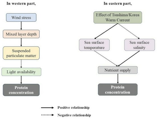
4.2. Major Environmental Controlling Factors for PRT of Each Part

Previous studies have identified several major factors influencing PRT concentration, including nutrient availability [47,48], light intensity [47,49], water temperature [50,51], and phytoplankton community [52,53]. Environmental conditions such as water temperature, nutrients, and irradiance are critical in controlling PRT concentration, with changes in the phytoplankton community considered less impactful [12,54].

Under low light conditions, PRT allocation tends to decrease, as more lipids and carbohydrates than PRT are synthesized under low light conditions [55,56,57]. In our study, a positive correlation between PAR and PRT was observed in the western part (Figure 7a). Interestingly, wind speed showed a negative correlation with PAR (Figure 7a). This could be attributed to the seasonal increase in wind stress during winter [58], deepening the MLD and causing sediment resuspension due to shallow water depth (average depth = 61 m) [59,60,61]. Consequently, sediment resuspension leads to an increase in SPM and a potential reduction in PAR [62,63,64]. During summer, stratification caused by low wind stress and warming SST likely reduces the nutrient supply to the surface layer [65,66], resulting in lower PRT concentrations. Suárez and Marañón [54] found that low PRT incorporation was due to low nutrient supply during summer stratification. Thus, a major controlling factor for PRT concentration in the western part could be the seasonal changes in physiochemical conditions (Figure 10a).

In the eastern part, a negative relationship between PRT and SST was observed, while a positive relationship was noted with SSS (Figure 7b). This region is characterized by the Tsushima/Korea Warm Current (TKWC), a branch of the Kuroshio Current [66,67,68,69,70]. Previous studies have demonstrated the negative correlation between PRT and SST [51,71,72]. This correlation can be attributed to the breakdown of PRT structures and interference with enzyme regulators at high temperatures [50]. Another contributing factor to this negative relationship could be low nutrient content in the TKWC. Previous studies indicate that the TKWC has low nutrient concentrations due to the effects of the nutrient-poor Kuroshio current [73,74]. Additionally, the TKWC exerts the most influence in the eastern part during summer and the least during winter [75,76,77]. Therefore, the nutrient-poor TKWC, originally derived from the Kuroshio current, may have had a more substantial influence on the eastern part during the summer when SST is high, leading to a decrease in PRT. An intriguing relationship between SSS and PRT was also found in this study. SSS in the eastern part of the NECS has been reported to be high in winter and low in summer [78,79]. Kim et al. [80] proposed that the deepening of the MLD brings saline halocline water into the mixed layer in autumn and winter, causing an increase in SSS. This mixing effect could potentially increase the supply of nutrients, leading to an increase in PRT concentration (Figure 10b).

In conclusion, the major controlling factors for PRT variation are different in the western and eastern parts of the NECS, despite similar seasonal patterns in PRT concentrations.

4.3. Spatial and Temporal Variation for PRT in the NECS

Throughout the observation period in this study, the western part generally exhibited higher PRT concentration than the eastern part (Figure 8). Despite no significant difference in light intensity between the eastern and western parts (t-test, p > 0.01), the eastern part had higher SST compared to the western part (t-test, p < 0.01). This temperature difference might have resulted in lower PRT concentration in the eastern part, as discussed in Section 4.2. Another potential factor is nutrient difference between the two regions. Previous field measurement studies have reported that PRT content increases under nutrient-rich conditions [17,81,82]. This increase is mainly due to PRT production depending on the availability of nitrogen substrates during photosynthesis [18,83,84]. Indeed, field-measured PRT concentrations in this study indicate that the western part had a higher nitrogen source compared to the eastern part (t-test, p < 0.01), consistent with previous studies [85,86,87]. Therefore, the relatively higher nutrient conditions likely contribute to the higher PRT concentration observed in the western part.

During the recent decade from 2012 to 2022, an earlier peak timing of PRT in spring was observed, especially in the western part of the NECS (Figure 9a). PRT was synthesized in large quantities during the spring bloom period of phytoplankton, as suggested by previous studies [57,82,88]. Indeed, the spring bloom timing of phytoplankton in the NECS has become increasingly earlier in recent years [89]. Therefore, this earlier peak timing of PRT in spring in this study might be attributed to the recent advancement of the bloom timing of phytoplankton in the western part of the NECS. Generally, spring blooms are known to be regulated by the availability of light due to the shoaling of the mixed layer depth below the critical depth [90]. However, concerning climate change, further studies are needed to confirm this relationship for a better understanding of the phytoplankton-associated biogeochemical process in the NECS.

5. Summary and Conclusions

In this study, we developed a regional algorithm to estimate PRT concentration in the NECS using SNPP-VIIRS satellite ocean color data, and our algorithm exhibited commendable performance (Figure 5). Identification of major environmental controlling factors for PRT concentration revealed distinctions between the western and eastern parts of the NECS (Figure 10). In the western part, PAR, SPM, MLD, and wind stress emerged as key influences, emphasizing the roles of light intensity, wind-induced mixing, and suspended particulate matter. In contrast, the eastern part, characterized by the TKWC, highlighted the importance of nutrient supply in regulating PRT concentration (Figure 10). These observed differences underline the biogeochemical complexity of the NECS. Specifically, the western part exhibits a light-dependent environment, while the eastern part relies on nutrients for PRT concentration. These findings provide valuable insights into the productivity of the NECS as a vital fishing ground, emphasizing the need for region-specific algorithms. Continuous field observations and algorithm refinement remain crucial for enhancing the robustness of PRT estimation. In conclusion, this study contributes to our understanding of regional algorithms for PRT estimation in the NECS, offering implications for environmental monitoring and sustainable fisheries management.

References

1. Xu, Q.; Wang, S.; Sukigara, C.; Goes, J.I.; Gomes, H.d.R.; Matsuno, T.; Zhu, Y.; Xu, Y.; Luang-on, J.; Watanabe, Y. High-resolution vertical observations of phytoplankton groups derived from an in-situ fluorometer in the East China Sea and Tsushima Strait. Front. Mar. Sci. 2022, 8, 756180. [Google Scholar] [CrossRef]
2. Hao, J.; Yuan, D.; He, L.; Yuan, H.; Su, J.; Pohlmann, T.; Ran, X. Cross-Shelf Carbon Transport in the East China Sea and Its Future Trend Under Global Warming. J. Geophys. Res. Oceans. 2024, 129, e2022JC019403. [Google Scholar] [CrossRef]
3. Kim, J.Y.; Kang, Y.S.; Oh, H.J.; Suh, Y.S.; Hwang, J.D. Spatial distribution of early life stages of anchovy (Engraulis japonicus) and hairtail (Trichiurus lepturus) and their relationship with oceanographic features of the East China Sea during the 1997–1998 El Niño Event. Estuar. Coast. Shelf. Sci. 2005, 63, 13–21. [Google Scholar] [CrossRef]
4. Bao, B.; Ren, G. Climatological characteristics and long-term change of SST over the marginal seas of China. Cont. Shelf Res. 2014, 77, 96–106. [Google Scholar] [CrossRef]
5. Whyte, J.N.C. Biochemical composition and energy content of 6 species of phytoplankton used in mariculture of bivalves. Aquaculture 1987, 60, 231–241. [Google Scholar] [CrossRef]
6. Kleppel, G.; Burkart, C. Egg production and the nutritional environment of Acartia tonsa: The role of food quality in copepod nutrition. ICES J. Mar. Sci. 1995, 52, 297–304. [Google Scholar] [CrossRef]
7. Kang, J.J.; Joo, H.T.; Lee, J.H.; Lee, J.H.; Lee, H.W.; Lee, D.; Kang, C.K.; Yun, M.S.; Lee, S.H. Comparison of biochemical compositions of phytoplankton during spring and fall seasons in the northern East/Japan Sea. Deep. Res. Part II Top. Stud. Oceanogr. 2017, 143, 73–81. [Google Scholar] [CrossRef]
8. Kang, J.J.; Jang, H.K.; Lim, J.-H.; Lee, D.; Lee, J.H.; Bae, H. Characteristics of different size phytoplankton for primary pro-duction and biochemical compositions in the Western East/Japan Sea. Front. Microbiol. 2020, 11, 3306. [Google Scholar] [CrossRef]
9. Mayzaud, P.; Chanut, J.P.; Ackman, R.G. Seasonal changes of the biochemical composition of marine particulate matter with special reference to fatty acids and sterols. Mar. Ecol. Prog. Ser. 1989, 56, 189–204. [Google Scholar] [CrossRef]
10. Duncan, R.J.; Petrou, K. Biomolecular composition of sea ice microalgae and its influence on marine biogeochemical cycling and carbon Transfer through polar marine food webs. Geoscience 2022, 12, 38. [Google Scholar] [CrossRef]
11. Scott, J. Effect of growth rate of the food alga on the growth/ingestion efficiency of a marine herbivore. J. Mar. Biol. Assoc. UK 1980, 60, 681–702. [Google Scholar] [CrossRef]
12. Lindqvist, K.; Lignell, R. Intracellular partitioning of 14CO2 in phytoplankton during a growth season in the northern Baltic. Mar. Ecol. Prog. Ser. 1997, 152, 41–50. [Google Scholar] [CrossRef]
13. Finkel, Z.V.; Follows, M.J.; Liefer, J.D.; Brown, C.M.; Benner, I.; Irwin, A.J. Phylogenetic diversity in the macromolecular composition of microalgae. PLoS ONE 2016, 11, e0155977. [Google Scholar] [CrossRef]
14. Geider, R.J.; MacIntyre, H.L.; Kana, T.M. A dynamic model of photoadaptation in phytoplankton. Limnol. Oceanogr. 1996, 41, 1–15. [Google Scholar] [CrossRef]
15. Morris, I. Photosynthetic products, physiological state, and phytoplankton growth. Can. Bull. Fish. Aquat. Sci. 1981, 210, 83–102. [Google Scholar]
16. Ríos, A.F.; Fraga, F.; Pérez, F.F.; Figueiras, F.G. Chemical composition of phytoplankton and particulate organic matter in the Ría de Vigo (NW Spain). Sci. Mar. 1998, 62, 257–271. [Google Scholar] [CrossRef]
17. Lee, S.H.; Kim, H.J.; Whitledge, T.E. High incorporation of carbon into proteins by the phytoplankton of the Bering Strait and Chukchi Sea. Cont. Shelf Res. 2009, 29, 1689–1696. [Google Scholar] [CrossRef]
18. Bhavya, P.S.; Kim, B.K.; Jo, N.; Kim, K.; Kang, J.J.; Lee, J.H.; Lee, D.; Lee, J.H.; Joo, H.T.; Ahn, S.H.; et al. A review on the macromolecular compositions of phytoplankton and the implications for aquatic biogeochemistry. Ocean Sci. J. 2019, 54, 1–14. [Google Scholar] [CrossRef]
19. Bae, H.; Lee, D.; Kang, J.J.; Lee, J.H.; Jo, N.; Kim, K.; Jang, H.K.; Kim, M.J.; Kim, Y.; Kwon, J.-I. Satellite-derived protein concentration of phytoplankton in the Southwestern East/Japan Sea. J. Mar. Sci. Eng. 2021, 9, 189. [Google Scholar] [CrossRef]
20. Parsons, T.R.; Maita, Y.; Lalli, C.M. A manual of chemical & biological methods for seawater analysis. Mar. Pollut. Bull. 1984, 15, 419–420. [Google Scholar]
21. Lowry, O.H.; Roserough, N.J.; Farr, A.L.; Randall, R.J. Protein measurement with the Folin phenol reagent. J. Biol. Chem. 1951, 193, 265–275. [Google Scholar] [CrossRef]
22. Uyanık, G.K.; Güler, N. A study on multiple linear regression analysis. Procedia Soc. Behav. Sci. 2013, 106, 234–240. [Google Scholar] [CrossRef]
23. Akinwande, M.O.; Dikko, H.G.; Samson, A. Variance inflation factor: As a condition for the inclusion of suppressor variables in regression analysis. Open J. Stat. 2015, 5, 754–767. [Google Scholar] [CrossRef]
24. Shrestha, N. Detecting multicollinearity in regression analysis. Am. J. Appl. Math. Stat. 2020, 8, 39–42. [Google Scholar] [CrossRef]
25. He, S.; Huang, D.; Zeng, D. Double SST fronts observed from MODIS data in the East China Sea off the Zhejiang–Fujian coast, China. J. Mar. Syst. 2016, 154, 93–102. [Google Scholar] [CrossRef]
26. Luo, Z.; Zhu, J.; Wu, H.; Li, X. Dynamics of the sediment plume over the Yangtze Bank in the Yellow and East China Seas. J. Geophys. Res. Oceans. 2017, 122, 10073–10090. [Google Scholar] [CrossRef]
27. Siswanto, E.; Tang, J.; Yamaguchi, H.; Ahn, Y.-H.; Ishizaka, J.; Yoo, S.; Kim, S.-W.; Kiyomoto, Y.; Yamada, K.; Chiang, C. Empirical ocean-color algorithms to retrieve chlorophyll-a, total suspended matter, and colored dissolved organic matter absorption coefficient in the Yellow and East China Seas. J. Oceanol. 2011, 67, 627–650. [Google Scholar] [CrossRef]
28. Son, S.; Wang, M. Ice detection for satellite ocean color data processing in the Great Lakes. IEEE Trans. Geosci. Remote Sens. 2017, 55, 6793–6804. [Google Scholar] [CrossRef]
29. Yoon, J.-E.; Son, S.; Kim, I.-N. Capture of decline in spring phytoplankton biomass derived from COVID-19 lockdown effect in the Yellow Sea offshore waters. Mar. Pollut. Bull. 2022, 174, 113175. [Google Scholar] [CrossRef]
30. O’Reilly, J.E.; Maritorena, S.; Mitchell, B.G.; Siegel, D.A.; Carder, K.L.; Garver, S.A.; Kahru, M.; McClain, C. Ocean color chlorophyll algorithms for SeaWiFS. J. Geophys. Res. Oceans. 1998, 103, 24937–24953. [Google Scholar] [CrossRef]
31. Tassan, S. Local algorithms using SeaWiFS data for the retrieval of phytoplankton, pigments, suspended sediment, and yellow substance in coastal waters. Appl. Opt. 1994, 33, 2369–2378. [Google Scholar] [CrossRef]
32. Wang, Y.; Liu, H.; Wu, G. Satellite retrieval of oceanic particulate organic nitrogen concentration. Front. Mar. Sci. 2022, 9, 943867. [Google Scholar] [CrossRef]
33. Hu, C.; Lee, Z.; Franz, B. Chlorophyll a algorithms for oligotrophic oceans: A novel approach based on three-band reflectance difference. J. Geophys. Res. Oceans. 2012, 117. [Google Scholar] [CrossRef]
34. Werdell, P.J.; Franz, B.A.; Bailey, S.W.; Feldman, G.C.; Vega-Rodriguez, M.; Guild, L.S.; De La Cour, J.L.; Boss, E.; Brando, V.E.; Dowell, M.; et al. Generalized ocean color inversion model for retrieving marine inherent optical properties. Appl. Opt. 2013, 52, 2019–2037. [Google Scholar] [CrossRef] [PubMed]
35. Ning, X.; Lin, C.; Su, J.; Liu, C.; Hao, Q.; Le, F. Long-term changes of dissolved oxygen, hypoxia, and the responses of the ecosystems in the East China Sea from 1975 to 1995. J. Oceanol. 2011, 67, 59–75. [Google Scholar] [CrossRef]
36. Ye, W.; Zhang, G.; Zhu, Z.; Huang, D.; Han, Y.; Wang, L.; Sun, M. Methane distribution and sea-to-air flux in the East China Sea during the summer of 2013: Impact of hypoxia. Deep Res. Part II Top. Stud. Oceanogr. 2016, 124, 74–83. [Google Scholar] [CrossRef]
37. Yamaguchi, H.; Ishizaka, J.; Siswanto, E.; Son, Y.B.; Yoo, S.; Kiyomoto, Y. Seasonal and spring interannual variations in satellite-observed chlorophyll-a in the Yellow and East China Seas: New datasets with reduced interference from high concentration of resuspended sediment. Cont. Shelf Res. 2013, 59, 1–9. [Google Scholar] [CrossRef]
38. Yoo, S.; Kong, C.E.; Son, Y.B.; Ishizaka, J. A critical re-assessment of the primary productivity of the Yellow Sea, East China Sea and sea of Japan/East Sea large marine ecosystems. Deep Res. Part II Top. Stud. Oceanogr. 2019, 163, 6–15. [Google Scholar] [CrossRef]
39. Liu, H.; Hu, S.; Zhou, Q.; Li, Q.; Wu, G. Revisiting effectiveness of turbidity index for the switching scheme of NIR-SWIR combined ocean color atmospheric correction algorithm. Int. J. Appl. Earth Observ. Geoinf. 2019, 76, 1–9. [Google Scholar] [CrossRef]
40. Jang, H.-K.; Youn, S.-H.; Joo, H.; Kang, J.-J.; Lee, J.-H.; Lee, D.; Jo, N.; Kim, Y.; Kim, K.; Kim, M.-J. First Estimation of the annual biosynthetic calorie production by phytoplankton in the Yellow Sea, South Sea of Korea, East China Sea, and East Sea. Water 2023, 15, 2489. [Google Scholar] [CrossRef]
41. Roy, S. Distributions of phytoplankton carbohydrate, protein and lipid in the world oceans from satellite ocean colour. ISME J. 2018, 12, 1457–1472. [Google Scholar] [CrossRef]
42. Zhang, C.-I.; Seo, Y.-I.; Kang, H.-J.; Lim, J.-H. Exploitable carrying capacity and potential biomass yield of sectors in the East China Sea, Yellow Sea, and East Sea/Sea of Japan large marine ecosystems. Deep Res. Part II Top. Stud. Oceanogr. 2019, 163, 16–28. [Google Scholar] [CrossRef]
43. Gao, L.; Wang, Y. Influences of environmental factors on the spawning stock-recruitment relationship of Portunus trituberculatus in the northern East China Sea. Acta Oceanol. Sin. 2021, 40, 145–159. [Google Scholar] [CrossRef]
44. Jo, N.; Kang, J.J.; Park, W.G.; Lee, B.R.; Yun, M.S.; Lee, J.H.; Kim, S.M.; Lee, D.; Joo, H.T.; Lee, J.H.; et al. Seasonal variation in the biochemical compositions of phytoplankton and zooplankton communities in the southwestern East/Japan Sea. Deep Res. Part II Top. Stud. Oceanogr. 2017, 143, 82–90. [Google Scholar] [CrossRef]
45. Chang, K.-I.; Zhang, C.-I.; Park, C.; Kang, D.-J.; Ju, S.-J.; Lee, S.-H.; Wimbush, M. (Eds.) Oceanography of the East Sea (Japan Sea); Springer International Publishing: Cham, Switzerland, 2016; ISBN 978-3-319-22719-1. [Google Scholar]
46. Longhurst, A. Seasonal cycles of pelagic production and consumption. Prog. Oceanogr. 1995, 36, 77–167. [Google Scholar] [CrossRef]
47. Morris, I.; Glover, H.E.; Yentsch, C.S. Products of photosynthesis by marine phytoplankton: The effect of environmental factors on the relative rates of protein synthesis. Mar. Biol. 1974, 27, 1–9. [Google Scholar] [CrossRef]
48. Kilham, S.S.; Kreeger, D.A.; Goulden, C.E.; Lynn, S.G. Effects of nutrient limitation on biochemical constituents of An-kistrodesmus falcatus. Freshw. Biol. 1997, 38, 591–596. [Google Scholar] [CrossRef]
49. Smith, A.; Morris, I. Pathways of carbon assimilation in phytoplankton from the Antarctic Ocean 1. Limnol. Oceanogr. 1980, 25, 865–872. [Google Scholar] [CrossRef]
50. Pirt, S.J. Principles of Microbe and cell cultivation, 1st ed.; Blackwell Scientific Publications: London, UK, 1975; pp. 115–117. [Google Scholar]
51. Lee, J.H.; Lee, D.; Kang, J.J.; Joo, H.T.; Lee, J.H.; Lee, H.W.; Ahn, S.H.; Kang, C.K.; Lee, S.H. The effects of different environmental factors on the biochemical composition of particulate organic matter in Gwangyang Bay, South Korea. Biogeosciences 2017, 14, 1903–1917. [Google Scholar] [CrossRef]
52. Rivkin, R.B.; Voytek, M.A. Photoadaptations of photosynthesis and carbon metabolism by phytoplankton from McMurdo Sound, Antarctica. 1. Species-specific and community responses to reduced irradiances. Limnol. Oceanogr. 1987, 32, 249–259. [Google Scholar] [CrossRef]
53. Wear, E.K.; Carlson, C.A.; Windecker, L.A.; Brzezinski, M.A. Roles of diatom nutrient stress and species identity in determining the short-and long-term bioavailability of diatom exudates to bacterioplankton. Mar. Chem. 2015, 177, 335–348. [Google Scholar] [CrossRef]
54. Suárez, I.; Marañón, E. Photosynthate allocation in a temperate sea over an annual cycle: The relationship between protein synthesis and phytoplankton physiological state. J. Sea Res. 2003, 50, 285–299. [Google Scholar] [CrossRef]
55. McConville, M.; Mitchell, C.; Wetherbee, R. Patterns of carbon assimilation in a microalgal community from annual sea ice, East Antarctica. Polar Biol. 1985, 4, 135–141. [Google Scholar] [CrossRef]
56. Smith, R.E.; Clement, P.; Cota, G.F.; Li, W.K. Intracellular photosynthate allocation and the control of arctic marine ice algal production 1. J. Phycol. 1987, 23, 124–132. [Google Scholar] [CrossRef]
57. Madariaga, I.; Fernández, E. Photosynthetic carbon metabolism of size-fractionated phytoplankton during an experimental bloom in marine microcosms. J. Mar. Biol. Assoc. UK 1990, 70, 531–543. [Google Scholar] [CrossRef]
58. Liu, K.-K.; Chao, S.-Y.; Lee, H.-J.; Gong, G.-C.; Teng, Y.-C. Seasonal variation of primary productivity in the East China Sea: A numerical study based on coupled physical-biogeochemical model. Deep Res. Part II Top. Stud. Oceanogr. 2010, 57, 1762–1782. [Google Scholar] [CrossRef]
59. Shi, W.; Wang, M. Satellite observations of the seasonal sediment plume in central East China Sea. J. Mar. Syst. 2010, 82, 280–285. [Google Scholar] [CrossRef]
60. Bian, C.; Jiang, W.; Quan, Q.; Wang, T.; Greatbatch, R.J.; Li, W. Distributions of suspended sediment concentration in the Yellow Sea and the East China Sea based on field surveys during the four seasons of 2011. J. Mar. Syst. 2013, 121, 24–35. [Google Scholar] [CrossRef]
61. Qiao, L.; Zhong, Y.; Wang, N.; Zhao, K.; Huang, L.; Wang, Z. Seasonal transportation and deposition of the suspended sediments in the Bohai Sea and Yellow Sea and the related mechanisms. Ocean Dyn. 2016, 66, 751–766. [Google Scholar] [CrossRef]
62. Lu, Z.; Gan, J.; Dai, M.; Cheung, A.Y. The influence of coastal upwelling and a river plume on the subsurface chlorophyll maximum over the shelf of the northeastern South China Sea. J. Mar. Syst. 2010, 82, 35–46. [Google Scholar] [CrossRef]
63. Zhao, L.; Guo, X. Influence of cross-shelf water transport on nutrients and phytoplankton in the East China Sea: A model study. Ocean Sci. 2011, 7, 27–43. [Google Scholar] [CrossRef]
64. Jiang, L.; Guo, X.; Wang, L.; Sathyendranath, S.; Evers-King, H.; Chen, Y.; Li, B. Validation of MODIS ocean-colour products in the coastal waters of the Yellow Sea and East China Sea. Acta Oceanol. Sin. 2020, 39, 91–101. [Google Scholar] [CrossRef]
65. Chen, Y.-l.L.; Chen, H.-Y.; Lee, W.-H.; Hung, C.-C.; Wong, G.T.; Kanda, J. New production in the East China Sea, comparison between well-mixed winter and stratified summer conditions. Cont. Shelf Res. 2001, 21, 751–764. [Google Scholar] [CrossRef]
66. Kim, D.; Choi, S.H.; Kim, K.H.; Shim, J.; Yoo, S.; Kim, C.H. Spatial and temporal variations in nutrient and chlorophyll-a concentrations in the northern East China Sea surrounding Cheju Island. Cont. Shelf Res. 2009, 29, 1426–1436. [Google Scholar] [CrossRef]
67. Lie, H.J.; Cho, C.H. On the origin of the Tsushima Warm Current. J. Geophys. Res. Oceans 1994, 99, 25081–25091. [Google Scholar] [CrossRef]
68. Gong, G.-C.; Chen, Y.-L.L.; Liu, K.-K. Chemical hydrography and chlorophyll a distribution in the East China Sea in summer: Implications in nutrient dynamics. Cont. Shelf Res. 1996, 16, 1561–1590. [Google Scholar] [CrossRef]
69. Shim, J.; Kim, D.; Kang, Y.C.; Lee, J.H.; Jang, S.-T.; Kim, C.-H. Seasonal variations in pCO2 and its controlling factors in surface seawater of the northern East China Sea. Cont. Shelf Res. 2007, 27, 2623–2636. [Google Scholar] [CrossRef]
70. Zhang, J.; Liu, S.; Ren, J.; Wu, Y.; Zhang, G. Nutrient gradients from the eutrophic Changjiang (Yangtze River) Estuary to the oligotrophic Kuroshio waters and re-evaluation of budgets for the East China Sea Shelf. Prog. Oceanogr. 2007, 74, 449–478. [Google Scholar] [CrossRef]
71. Tomaselli, L.; Giovannetti, L.; Sacchi, A.; Bocci, F. Effects of temperature on growth and biochemical composition in Spirulina platensis strain M2. In Algal Biotechnology; Stadler, T., Mellion, J., Verdus, M., Karamanos, Y., Morvan, H., Christiaen, D., Eds.; Elsevier Applied Science: London, UK, 1988; pp. 303–314. [Google Scholar]
72. Oliveira, M.; Monteiro, M.; Robbs, P.; Leite, S. Growth and chemical composition of Spirulina maxima and Spirulina platensis biomass at different temperatures. Aquac. Int. 1999, 7, 261–275. [Google Scholar] [CrossRef]
73. Jiao, N.; Yang, Y.; Hong, N.; Ma, Y.; Harada, S.; Koshikawa, H.; Watanabe, M. Dynamics of autotrophic picoplankton and heterotrophic bacteria in the East China Sea. Cont. Shelf Res. 2005, 25, 1265–1279. [Google Scholar] [CrossRef]
74. Chen, C.-T.A. Chemical and physical fronts in the Bohai, Yellow and East China seas. J. Mar. Syst. 2009, 78, 394–410. [Google Scholar] [CrossRef]
75. Teague, W.J.; Jacobs, G.A.; Perkins, H.T.; Book, J.W.; Chang, K.I.; Suk, M.S. Low-frequency current observation in the Korea/Tsushima Strait. J. Phys. Oceanogr. 2002, 32, 1621–1641. [Google Scholar] [CrossRef]
76. Ma, C.; Wu, D.; Lin, X.; Yang, J.; Ju, X. On the mechanism of seasonal variation of the Tsushima Warm Current. Cont. Shelf Res. 2012, 48, 1–7. [Google Scholar] [CrossRef]
77. Seung, Y.H. Some dynamical issues about the Tsushima Warm Current based on bibliographical review. Sea J. Korean Soc. Oceanogr. 2019, 24, 439–447. [Google Scholar]
78. Ichikawa, H.; Chaen, M. Seasonal variation of heat and freshwater transports by the Kuroshio in the East China Sea. J. Mar. Syst. 2000, 24, 119–129. [Google Scholar] [CrossRef]
79. Chu, P.; Chen, Y.C.; Kununaka, A. Seasonal variability of the Yellow Sea/East China Sea surface fluxes and thermohaline structure. Adv. Atmos. Sci. 2005, 22, 1–20. [Google Scholar] [CrossRef]
80. Kim, S.B.; Lee, J.H.; de Matthaeis, P.; Yueh, S.; Hong, C.S.; Lee, J.H.; Lagerloef, G. Sea surface salinity variability in the East China Sea observed by the Aquarius instrument. J. Geophys. Res. Oceans 2014, 119, 7016–7028. [Google Scholar] [CrossRef]
81. Boëchat, I.G.; Giani, A. Seasonality affects diel cycles of seston biochemical composition in a tropical reservoir. J. Plankton Res. 2008, 30, 1417–1430. [Google Scholar] [CrossRef]
82. Kim, B.K.; Lee, J.H.; Joo, H.; Song, H.J.; Yang, E.J.; Lee, S.H.; Lee, S.H. Macromolecular compositions of phytoplankton in the Amundsen Sea, Antarctica. Deep Res. Part II Top. Stud. Oceanogr. 2016, 123, 42–49. [Google Scholar] [CrossRef]
83. Fabiano, M.; Povero, P.; Danovaro, R. Distribution and composition of particulate organic matter in the Ross Sea (Antarctica). Polar Biol. 1993, 3, 525–533. [Google Scholar] [CrossRef]
84. Danovaro, R.; Dell’Anno, A.; Pusceddu, A.; Marrale, D.; Della Croce, N.; Fabiano, M.; Tselepides, A. Biochemical composition of pico-, nano-and micro-particulate organic matter and bacterioplankton biomass in the oligotrophic Cretan Sea (NE Mediterranean). Prog. Oceanogr. 2000, 46, 279–310. [Google Scholar] [CrossRef]
85. Chen, C.-T.A. Distributions of nutrients in the East China Sea and the South China Sea connection. J. Oceanol. 2008, 64, 737–751. [Google Scholar] [CrossRef]
86. Kim, D.-S.; Choi, S.-H.; Kim, K.-H.; Kim, C.-H. The distribution and interannual variation in suspended solid and particulate organic carbon in the northern East China Sea. Ocean Polar Res. 2009, 31, 219–229. [Google Scholar] [CrossRef]
87. Kim, Y.; Youn, S.-H.; Oh, H.J.; Kang, J.J.; Lee, J.H.; Lee, D.; Kim, K.; Jang, H.K.; Lee, J.; Lee, S.H. Spatiotemporal variation in phytoplankton community driven by environmental factors in the northern East China Sea. Water 2020, 12, 2695. [Google Scholar] [CrossRef]
88. DiTullio, G.R.; Laws, E.A. Estimates of phytoplankton N uptake based on 14CO2 incorporation into protein. Limnol. Oceanogr. 1983, 28, 177–185. [Google Scholar] [CrossRef]
89. Wu, Y.; Zhu, H.; Dang, X.; Cheng, T.; Yang, S.; Wang, L.; Huang, L.; Cui, X. Spatial-temporal change of phytoplankton biomass in the East China Sea with MODIS data. J. Ocean Univ. China 2021, 20, 454–462. [Google Scholar] [CrossRef]
90. Sverdrup, H. On conditions for the vernal blooming of phytoplankton. J. Cons. Int. Explor. Mer. 1953, 18, 287–295. [Google Scholar] [CrossRef]
Figure 1. Study area in the northern East China Sea (NECS). Red circles, blue squares, yellow triangles, green diamonds, and cyan inverted triangles indicate the stations measured in 2018, 2019, 2020, 2021, and 2022. Black lines indicate domains for the western and the eastern parts of the NECS.
Remotesensing 16 00829 g001
Figure 2. Boxplots of in situ data with seasonal variation. The green triangle represents the mean value of the data, and the red line within the boxplot represents the median value of the data. (a) Total chlorophyll-a (Chla), (b) Particulate organic nitrogen (PON), and (c) Proteins (PRT). The bars at the top of the figure represent the results of t-tests conducted between the datasets, where *** denotes p < 0.001, ** denotes p < 0.01, and * denotes p < 0.05.
Remotesensing 16 00829 g002
Figure 3. Validation result of the model-based PRT algorithm with in situ PRT data. Black dashed line represents 1:1 line.
Remotesensing 16 00829 g003
Figure 4. Comparison of in situ Chla and PON with SNPP-VIIRS derived Chla and PON concentrations for different models. (a) switching Chla algorithm, (b) NASA OC3 Chla algorithm, (c) Tchl_Tchl2i Chla algorithm, (d) switching PON algorithm, (e) CI-using PON algorithm, and (f) a(486) PON algorithm. Both axes in all graphs are transformed to log10. The colors plotted on scatterplots represent values of nLw551 as an indicator of turbidity. The black dashed lines represent 1:1 line.
Remotesensing 16 00829 g004
Figure 5. Linear relationship between satellite-estimated PRT and in situ PRT concentrations. Black dashed line represents the 1:1 line.
Remotesensing 16 00829 g005
Figure 6. Validation results for the two PRT algorithms in this study (sky blue circles) and Bae et al. [19] (orange triangles). Black dashed line represents 1:1 line. The linear regression lines between in situ PRT and the satellite-estimated PRT are depicted by the sky blue and orange solid lines, respectively. The shaded areas in sky blue and orange, respectively, represent the 95% prediction intervals for this study and the East Sea algorithm.
Remotesensing 16 00829 g006
Figure 7. Composite plots for one-to-one comparison between satellite-estimated PRT and various environmental parameters (bottom-left half) and Pearson’s correlation coefficient heatmap (r, top-right half) in (a) the western and (b) eastern parts of the NECS. The scatter plot color darkens progressively from spring to winter, where orange denotes the western part and green denotes the eastern part. ** p < 0.01.
Remotesensing 16 00829 g007
Figure 8. Climatological seasonal mean distribution of PRT concentration in the NECS from 2012 to 2022.
Remotesensing 16 00829 g008
Figure 9. The heatmap images of 8-day time series PRT concentration from 2012 to 2022 in (a) the western and (b) eastern parts of the NECS.
Remotesensing 16 00829 g009
Figure 10. Schematic models for PRT concentration variations in (a) the western and (b) eastern parts of the NECS. (a) MLD stands for Mixed layer depth, SPM represents Suspended particulate matter, and PRT refers to Protein. (b) TKWC (red line) denotes the Tsushima/Korea Warm Current, while SST and SSS represent Sea surface temperature and Sea surface salinity, respectively.
Remotesensing 16 00829 g010aRemotesensing 16 00829 g010b