
An Effective Onboard Cold-Sky Calibration Strategy for Spaceborne L-Band Synthetic Aperture Radiometers

1
Institute of Remote Sensing Satellite, CAST, Beijing 100094, China
2
Advanced Space Technology Laboratory, Nanjing University of Aeronautics and Astronautics, Nanjing 211106, China
3
Faculty of Information Science and Engineering, College of Marine Technology, Ocean University of China, Qingdao 266100, China
*
Author to whom correspondence should be addressed.
Remote Sens. 2024, 16(6), 971; https://0-doi-org.brum.beds.ac.uk/10.3390/rs16060971
Submission received: 24 December 2023
/
Revised: 6 March 2024
/
Accepted: 8 March 2024
/
Published: 10 March 2024
(This article belongs to the Special Issue Microwave Passive Remote Sensing of Sea Surface Temperature, Salinity and Wind Vector)
Abstract
:The L band frequency shows high sensitivity to sea surface salinity. More stable brightness temperature (TB) measurements are required for L-band radiometers to reduce salinity retrieval errors than for high-frequency radiometers. Due to the complexity of L-band synthetic aperture radiometers, a carefully selected cold-sky target should be viewed using an L-band synthetic aperture radiometer for the purpose of absolute TB calibration since the celestial sky is relatively well characterized and stable in the L band. A novel, effective cold-sky calibration strategy is presented in this paper. The strategy of cold-sky calibration of the synthetic aperture radiometer is applied when and where the antenna main lobe points to the ‘flat’ celestial sky, and the impact of each type of foreign source, such as the sun or moon, on visibility values should be minimized in the meantime. Additionally, antenna thermal stability is also considered, which can cause antenna deformation, and the antenna patterns are affected. A high-precision and high-fidelity simulator is built for the cold-sky calibration optimized strategy. The orbital beta angle is introduced to characterize the variation in space environment temperatures. A planet that is considered spherical in shape requires significantly less computation than an ellipsoid one in the simulator. The trade-off study results for the planet shape assumption in the cold-sky calibration simulator are presented. Finally, the calibration uncertainty and performance are assessed.
1. Introduction
Cold-sky calibration for spaceborne L-band synthetic aperture radiometers is essential for reducing salinity retrieval errors. The system response to known controlled signals, so-called calibration, is key to the success of the radiometer mission. In order to monitor and forecast sea surface salinity, the assimilation of different radiometer satellites is used to reduce ocean analysis errors, which requires high-quality calibration technology. To support this goal, brightness temperature absolute calibration is the key technology used to obtain high-precision data. The absolute calibration of synthetic aperture radiometers is performed by viewing the deep-sky scene [1]. The calibration stages can be divided into pre-launch calibration and post-launch calibration. During the operation of the satellite, the offset bias of the instruments can introduce measurement errors into the visibilities of synthetic aperture radiometers, resulting in deviation between on-ground characterizations and in-flight ones if the pre-launch calibration coefficient continues to be used. Therefore, in order to avoid greater impact on subsequent data products at all levels, in-orbit cold-sky calibration of the radiometer sensors is required to eliminate systematic deviations and improve data accuracy.
Periodic cold-sky observation maneuvers are performed over a specific part of Earth’s surface to evaluate relative and absolute calibration post-launch, such as Jason3 radiometers, SMOS, Aquarius, and SMAP radiometers [1,2,3,4,5,6]. The radiometer antenna patterns’ information can be refined by cold-sky maneuvers. For example, the SMAP radiometer antenna points to the cold sky near the Amazonian rainforest, and the backlobe of the antenna observes a transition from ocean to rainforest to correct antenna backlobe spillover. Cold-sky calibration can also be used to calibrate the internal noise diode [2]. The modeled values over cold-sky targets are compared with the measurements of the radiometer for quantification. The simulators of radiometers for cold-sky calibration can be used for calibration program design, which should consider many factors, such as the proportion of land and sea in the antenna pattern and the ground track over the celestial sky [7]. The number of antennas in a synthetic aperture radiometer is much larger than in a real aperture radiometer. For example, the Y-shaped 2D array of MIRAS is formed by three arms about 4.5 m long, with 23 equally spaced antennas each [8]. Additionally, the simulation of a synthetic aperture radiometer for its cold-sky calibration takes much more time, and the quantity is calculated using the traversing method. The influence of the space environment is not considered in traditional cold-sky calibration tactics. In this paper, an effective strategy for the cold-sky calibration of synthetic aperture radiometers is proposed, with consideration of the effect of external thermal environmental variation. The error of the assumption of a spherical Earth is also quantified, which can be used to simplify the simulator for the cold-sky calibration scheme and achieve high-fidelity results with very few computational resources. The offsets in the TB caused by the antenna pattern error between the on-ground and in-flight measurements are assessed, which are mainly due to the influence of antenna uncertainty caused by the space environment alternating between cooling and heating.
2. Cold-Sky Calibration Simulator
Synthetic aperture radiometers can obtain high-sensitivity and large-spatial-domain measurements of Earth’s surface simultaneously. The different interference baselines are performed by cross-correlating pairs of antenna elements. The visibility function can be formed based on the interference patterns from reasonable spatially distributed antennas. A Fourier synthesis process of the cross correlations is performed through Equation (1), where ξ,η represent the direction cosines and are defined with respect to the angles in the antenna reference frame, Ω is the solid angle of the antennas, TB is the simulated brightness temperature of the scene, Trec is the estimated equivalent noise temperature of the receivers, and F(ξ,η) is the normalized antenna pattern [8].
The brightness temperature image reconstruction of the synthetic aperture radiometer can be approximately computed using the inverse Fourier transform of the visibility function, as shown below:
The simulator is a forward algorithm [9], which can compute the brightness temperature of the antenna, given the parameters of the surface and surrounding environment (e.g., the ocean, land, sun, moon, and celestial sky) [10,11]. The effects of propagation, attenuation, its own emitted radiation into the atmosphere, and the radiation coming from the Earth’s surface are considered in the simulator. The brightness temperature of the sources, which, considered here, are the ocean and land surfaces over Earth, the sun/moon, and the celestial sky background, are modeled using real historical data or empirical data. The effects of the troposphere and Faraday rotation of L-band signals are modeled in the simulator, too. The antenna pattern of each feed horn or reflector antenna with a common feed horn is used to select the appropriate area that meets the requirements for cold-sky calibration. The optimum conditions are based on those described in detail in [10] and some new considerations. The brightness temperature of the target’s scene at each antenna is first to be calculated, and then the synthetic images can be calculated. Earth is assumed to be spherical and ellipsoid in shape, respectively, to obtain the radiation contribution from Earth’s surface because the cost of calculation of the Earth ellipsoid model is much more than the spherical model when simulating satellite operation on board. Even a whole year’s worth of orbital data need to be looked through to find a suitable cold-sky calibration time and location. It is necessary to trade off efficiency and accuracy for the run time of the simulator. The angle pointing error brought by the spherical model is about 0.2 degrees against the World Geodetic System of 1984 (WGS-84) Earth ellipsoid model [12]. The approximation error of spherical and ellipsoid models is calculated and evaluated, and the inversed brightness temperature of the synthetic aperture radiometer can be given to show the effect of cold-sky calibration.
2.1. The Antenna Temperature (Ta) of Each Antenna
The salinity of the sea surface can be monitored from space by a microwave radiometer in the L-band, which requires higher sensitivity and accuracy than other radiometers. The main lobe of the antenna looks toward a uniform cold-sky scene with a low brightness temperature while cold-sky calibration is performed, which is used for the radiometer’s absolute calibration and instrument stability test. The scene below the satellite can have an effect on the accuracy of the calibration reference temperature because the brightness temperature of Earth’s surface is different, as shown in Figure 1. The brightness temperature of the land or ocean scene is much higher than the cold-sky scene, which impacts the Ta of the antenna through the back lobes [9]. The antenna temperatures of the radiometers due to emissions from all sources are calculated using the equation described below [9,10]:
where Ta is the brightness temperature of the antenna, G is the antenna directivity pattern, (θ, φ) is the incident direction, and is the effective brightness temperature of the directions. The integral is performed over all incident directions of the domain .
An imaging geometry of the look vector from a given antenna and its rotation for cold-sky calibration are given in Figure 2. The ‘target’ can be the ocean, the sky, the land, and the sun or moon. A local coordinate system is represented by (, , ) in the figure. The look vector from a given antenna is defined by:
where θ is the elevation angle, and φ is the azimuth angle of a spherical coordinate system. (--) is a rectangular coordinate system, used to describe the antenna orientation, whose relationship with the spacecraft body coordinate system can be given by:
where AT = (R1(roll)·R2(pitch) ·R3(yaw))−1 is made of the attitude angle of the satellite, which is the rotational angle value, as shown in Figure 2. The attitude angle of the spacecraft can be measured by the Flight Control System. R(·) is the Euler rotation matrix about the corresponding axis, and yaw, roll, and pitch stand for the rigid body S/C roll, pitch, and yaw angle, respectively. Me is the installation matrix of the antenna position on board.
In order to obtain the brightness temperature when the satellite is flying forward, the scene into the radiometer’s field of view (FOV) is divided into four parts: the sun, the moon, the celestial sky, and Earth. A typical relative orientation of the sun, moon, and satellite when the satellite operates on a sun-synchronous orbit is shown in Figure 1. The antenna brightness temperature is shown in Equation (6):
where G is the antenna pattern, is the brightness temperature contribution from the back of the antenna that faces Earth during cold-sky calibration, and and are the sky, sun, and moon parts of the field of view, respectively.
2.2. Moon and Sun’s Radiation during Calibration
The estimation of the angle of the sun or moon with respect to the array boresight is critical for calibration. The total antenna temperature and the observed standard deviation error of the celestial sky measurements are affected by the sun’s position in SMOS [5]. The brightness temperature drifts, although the receiver temperature does not change much. Therefore, the influence of the sun/moon on the synthetic aperture radiometer is one of the factors that must be considered in external calibration. In a given epoch, the position of the spacecraft in an Earth-fixed coordinate system is Ps (x, y, z), and the velocity is Vs (Vx, Vy, Vz), as shown in Figure 3. The + Z axis of the antenna of the radiometer points to the ground, and the +X axis is oriented towards the track direction when the satellite is flying forward. According to the sun/moon vectors SM(x, y, z), the angle θa = f(Poz, SM) can be obtained, that is, the angle between the sun/moon vector and + Z axis [6]. Poz is the +Zs axis direction of the spacecraft body frame in the Earth-fixed coordinate system, and it can be obtained by the attitude variations (roll, pitch, or yaw) from spacecraft data. The SM vector originates from where Poz originates. The angle between the sun/moon vector and the + X axis of the antenna coordinate system is φa = f(Pox, Projxoy_plane(SM)) in the spherical coordinate system, where Projxoy_plane(·) is the vector projection function to the XOY plane and . The sun/moon reflection location on the ground is described in the following equation, assuming that Earth’s semi-major axis is ae, the semi-minor axis is be, and the position of the reflection point Pref can be written in the form of the following equations. This situation calls for a more realistic elliptical model for Earth.
The angle between the reflected sun/moon direction and the antenna boresight can be calculated by solving the position of the sun/moon reflection at the intersection of the grid points with the WGS-84 Earth ellipsoid.
Figure 4 shows the direct sun/moon and reflected sun angles entering into the antenna’s field of view in a complete year for a typical sun-synchronous orbit. The Y axis of the antenna reference frame is perpendicular to the orbital plane, and the X axis is tilted 30 degrees upward from the velocity vector of the satellite. Figure 5 shows the brightness temperature map of the sun with an antenna pattern like SMOS antennas [13]. The brightness temperature of the geometric location of the satellite position is calculated by one antenna element.
2.3. Cosmic Background Radiation during Calibration
Sufficiently stable targets such as galactic poles are used in external calibration measurement, which can provide an image level of about 3.5 K with spatial homogeneity over large regions and good temporal stability [1,3,4,8]. Using the deep-sky view, the absolute calibration of the radiometer is performed, whose procedure is called ‘flat-target transformation’ [14]. The bright temperature map of the L-band cold sky is established in both declination and right ascension in equatorial coordinates using the J2000.0 or B1950 system [15]. The brightness temperature of the cold-sky target is rather constant for both polarizations [3,4]. The nominal SMOS sky map is derived from the Reich and Testori continuum map [15]. During the cold-sky view, the main lobes of the antenna look up toward the cold sky and the back lobes look toward Earth, and each antenna of the synthetic aperture radiometer moves along the spacecraft’s orbit. The components that contribute to the BT of the antenna FOV can be obtained by the position of the satellite, which is given by the ellipsoid equation in Cartesian coordinates in an Earth-centered inertial reference frame, and the Sky Tb can be obtained by integrating over the antenna pattern. The area observed by the radiometer antenna is converted into right ascension and declination under the corresponding coordinate system, and the cold-sky scene is interpolated to the image observed by the radiometer. The contribution of the celestial sky is obtained at each point of the satellite. The cross-correlations between the pairs of antenna elements are carried out to synthesize the visibility function.
2.4. Effect of Antenna Thermal Distortion
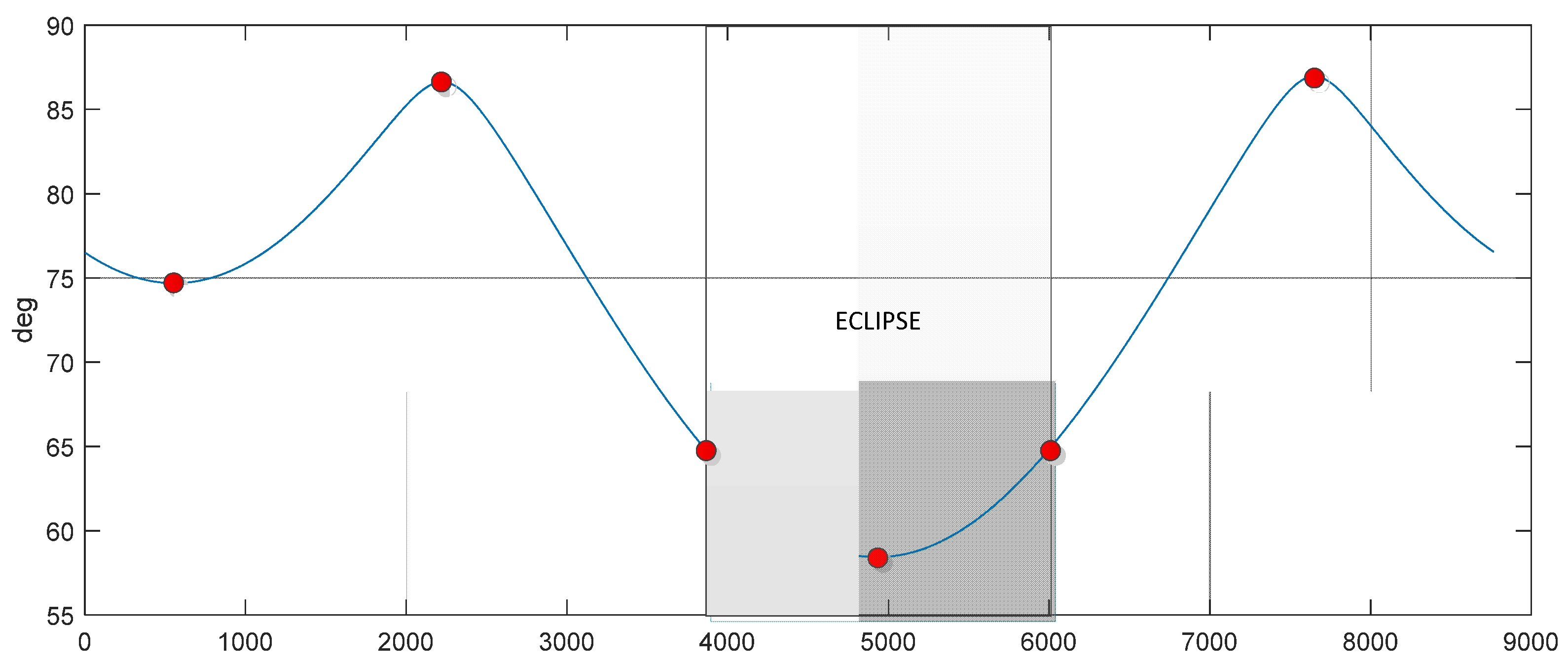
In order to improve the fidelity of the simulation for cold-sky calibration design, a parameter that can depict the effect of the space environment, especially the thermal conditions, should be introduced into the procedure of the cold-sky calibration strategy. The beta angle (β), which is the angle between the solar vector and the orbital plane, is usually used to perform thermal analysis and design. Thereby, it can be used as the parameter that depicts the thermal environment variation around the orbit. The worst thermal environments happen at higher beta angles when the sun is more fully incident on the feed horn, and the mutation of the thermal environment happens at the red dot area, as shown in Figure 6. The thermal analysis results of the radiometer antenna can be obtained from the material properties of the antenna and the thermal model, which is traditionally modeled by the beta angle [16]. The spaceborne radiometer antenna’s gain is affected by the variation in the physical temperature, whose effect on cold-sky calibration can be very large. When the temperatures of the antennas change periodically as the satellite flies, geometrical errors of the antennas are generated periodically. The red dots in Figure 6 show both the inflection point of the beta angle curve and the moment when the eclipse seasons begin and end, where the temperature changes extensively, and the worst-case thermal stability [16]. By being combined with the thermal expansion coefficient of the antenna material and antenna temperatures, the antenna deformation can be quantitatively established, and the relationship between the beta angle and the gain variation of the antenna can be modeled as a look-up table before launch. In-orbit antenna pattern verification is based on the flat target response of the cold-sky scene during external observation [1]. The antenna pattern errors due to thermal distortion will reduce the effect of flat target transformations. Therefore, the space environment of the satellite operating on should be paid attention to when choosing opportunities for cold-sky calibration. The beta angle can be used as a parameter depicting the space environment’s impact.
3. Strategy of Cold-Sky Calibration for Synthetic Aperture Radiometers
It is necessary that the location of the inverted position of the synthetic aperture radiometer satellite for cold-sky viewing be well chosen to obtain an accurate calibration. The effective selection of an optimized cold-sky calibration location, a calibration area based on the maximum brightness temperature stability for each antenna, and consideration of the thermal environmental variation around the orbit are critical. Therefore, the strategy of cold-sky calibration for synthetic aperture radiometer satellites is depicted as follows:
- The location should be as far away from land or ice as possible, while the attitude errors of the satellite are considered. The FOV of the synthetic aperture radiometer is far wider than the real aperture radiometer, and the brightness temperature of the land is larger than the brightness temperature of the ocean. Therefore, the contribution from the Earth’s surface can cause brightness temperature readings that are several Kelvins higher from the back lobes of the antenna. The brightness temperature of the ocean is generally considered to be about 100 K in the model. The brightness temperature of the land is about 250 K, the brightness temperature of the celestial sky is approximated by 2.7 K~10 K, and the brightness temperature of the atmosphere is generally 2.5 K [10,11]. The land contribution via the antenna back lobes should be minimized; that is, the land fraction should be as little as possible.
- The location should be far from the plane of the galaxy, moon, and sun. Due to Gibbs ringing in the synthetic aperture radiometer, it will cause some changes in the signal observed if foreign sources radiate into the field of view of the antennas, which can lead to a large error in antenna brightness temperature. When flat target transformation (FTT) is performed, this deviation in the cold-sky observation will be considered the antenna error. In addition, the impact of the antenna pattern model biases can be introduced and wrongly re-calibrated. Therefore, calibration should be performed where the brightness temperature of the antenna is the most stable. The sun and other external sources should not enter the main lobes of the antenna, avoiding strong fluctuations in the brightness temperature.
- The antenna’s thermal stability should also be considered in the strategy. According to the emulated relationship between antenna thermal deformation and antenna pattern changes at the pre-launch phase, the appropriate β value for cold-sky observation is determined by minimizing the antenna pattern variation. If the β angle meets the requirements, the corresponding time is suitable for cold-sky calibration. Once the satellite orbit is determined, the antenna temperature field distribution can be calculated from the orbital beta angle (β angle) and the antenna thermal parameters [17]. The antenna’s thermal parameters are known by the material properties, so the temperature field distribution is only determined by the beta angle, that is, FA(x,y) = f(β). The antenna thermal deformation can also be determined by f(β). Then, according to the acceptable range of antenna pattern error, the acceptable β range of external calibration can be determined. A look-up table can be obtained before the satellite is launched by simulation. The red dot area in Figure 6 should be avoided.
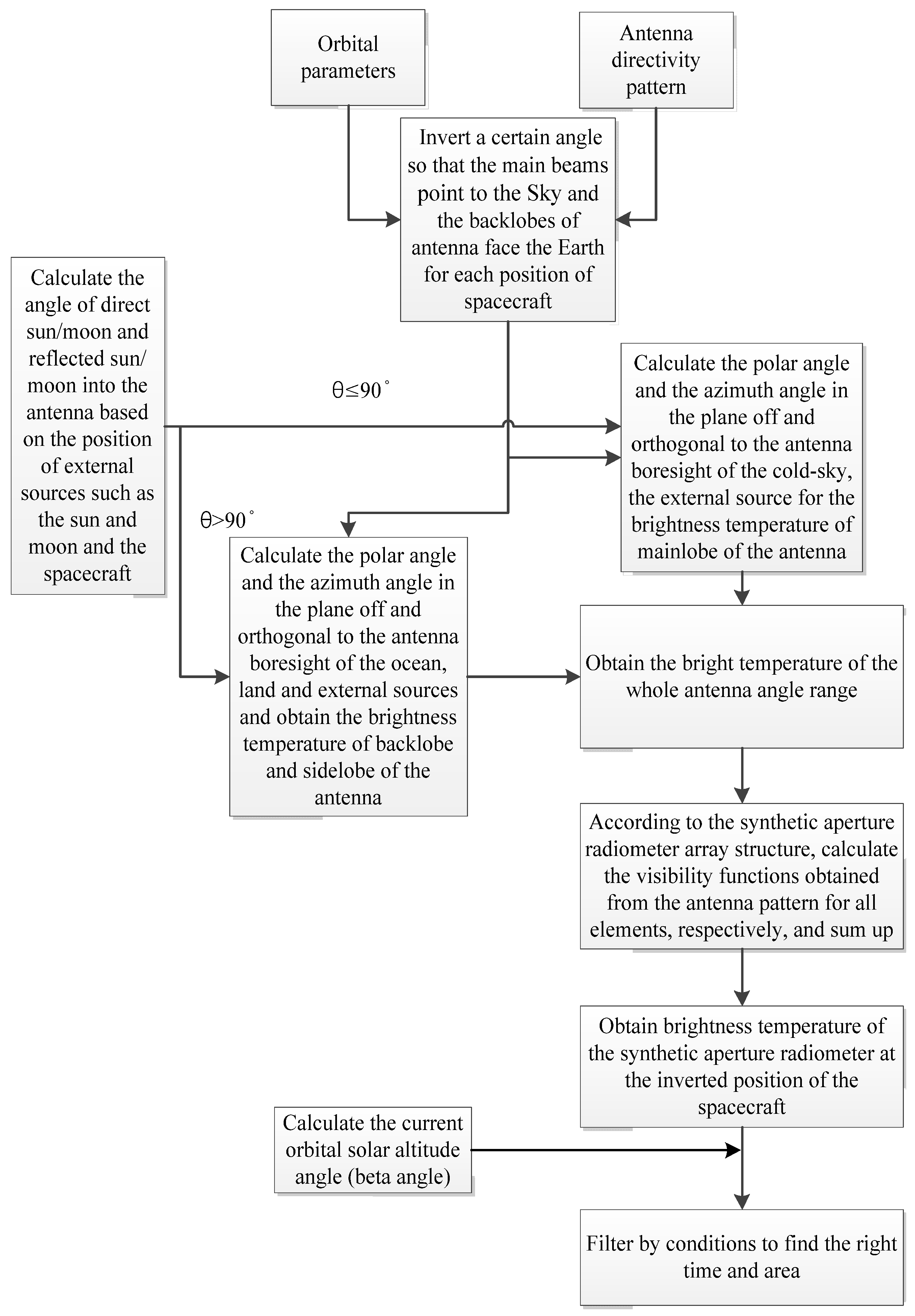
Based on all the above principles, the time and location for cold-sky calibration can be selected by the following process, as shown in Figure 7.
Finally, the optimized region and time for cold-sky calibration can be found according to the above conditions. The real-time geometrical relationships of the direct/reflected sun vector, the cold-sky region, and the satellite radiometer antenna can be determined by the method mentioned in Section 2. The visibility function of the synthetic aperture radiometer is performed through the process of cross-correlation with every pair of elements in the array [9]. The angle (θa, φa) of the relationship of the direct/reflected sun vector, the cold-sky region, the Earth–sky horizon, the land–ocean fraction, and the director cosine (ξ, η) domain is established, as shown in the following equation. The brightness temperature image reconstruction of the synthetic aperture radiometer of the scene is formed by taking the inverse Fourier transform.
Due to the variations and the effect of the external thermal influence and other space environment factors after launching, there are some differences between on-ground antenna patterns and the in-flight antenna patterns. The accuracy of synthetic aperture radiometer cold-sky calibration is affected by visibility function differences from a flat target, which has a brightness temperature error against a known cold (deep)-sky scene because of the effect of antenna pattern characterization errors. By adding some errors between the on-ground characterizations and in-flight ones, the pixel bias can be evaluated by the brightness temperature of the ‘in-flight’ cold-sky scene and the ‘real’ cold-sky scene. The impact of the antenna error on cold-sky calibration performed using the strategy in Figure 7 can be determined via the following formula:
4. Results and Discussion
An antenna pattern similar to the one in [13] is used for the selection of an optimized calibration location and the brightness temperature calculation for an L-band synthetic aperture radiometer. The results are shown as follows.
Figure 8a shows the antenna brightness temperatures for the radiometer antenna beams when the cold-sky maneuver is emulated. The spacecraft rotates over 180° from its normal Earth-observing attitude to an orientation pointing toward the celestial sky, where the radiometer antennas are looking into the sky. Each point in the figure represents the projection of the center of the field of view of the antenna at each satellite position on the ground, and the color represents the brightness temperature value (unit: K) of the single antenna obtained while inverting the spacecraft here. The ground track, colored green, shows the lower brightness temperature, while the main beam of the antenna is looking toward the sky at this time, and Earth’s surface is the ocean. The yellow and red colors show the brightness temperature change as the spacecraft crosses from land to ocean or otherwise. The integral of the power incident on the antenna is relatively low and constant when the satellite flies over an ocean far from land. The signal emitted from all kinds of sources surrounding the antenna is very stable at the same time. The dominant element of the signal is the direct emission of the sky, which enters the main lobe of the antenna. Additionally, the timing is suitable for the cold-sky maneuver from Earth’s surface, and the direct emission from upwelling from the atmosphere into the back lobes of the antenna and the sum of the sun and moon entering into the side lobes of the antenna are also small and stable in the meantime. There are also some differences between the descending pass and the ascending pass at the same inverted position, as shown in this figure. For example, the antenna temperatures at the same location during the ascent orbit are slightly lower than the antenna temperatures at the descent orbit in the Pacific region.
The appropriate geometry for the Aquarius CSC is chosen by the threshold corresponding to a weighted land fraction between 0.02% and 0.03% [9]. Figure 8b shows the results of the area selected by the criterium of a weighted land fraction <0.03%, based on a previous study, and the radiometer system operates on the sun-synchronous orbit parameter with an equatorial altitude of about 600 km. The figure shows the region with minimal interfering radiation from Earth among the data from 15 January 2021 04:24:00.000 to 19 January 2021 08:24:00.000. The red dot represents a suitable region to perform cold-sky calibration.
Although the spherical approximation of the Earth model is simple and fast to implement in the computation, it can introduce some significant errors in geolocations and local incidence angles [9]. The antenna temperature Ta bias between the Earth ellipsoid model and the simplified spherical model in the cold-sky observation of the radiometer system is simulated in Figure 9. The differences are very apparent from the comparison of these two Earth models, especially when the spacecraft flies across the coastline, which is relatively larger than 1 K. For example, significant errors can happen at some land–ocean crossing geolocations, such as the ocean area at 60 degrees south latitude near the South Pole, the Bering Strait, the ocean near the Amazon forest, and so on. Therefore, the simplified spherical model of Earth is not suitable for antenna spillover or sidelobe calibration mode design, which can lead to significant errors, although the computation is efficient. As for cold-sky calibration design over an open-ocean area, the simplified spherical model of Earth can be used to improve efficiency.
The spacecraft is usually kept inverted into the sky for a few minutes during cold-sky calibration. For example, the maneuvers before and after the external calibration measurement period each take about 20 min on SMOS [1]. The duration of the external calibration mode is less than 10 min; the actual measurements should, therefore, take less than 60 min. This duration value is further restricted to the pointing stability holding time, as shown in [1]. Assuming that the cold-sky observation time is 10 min, the single-antenna brightness temperature observation results are given in Figure 10a under the above three selection conditions. The brightness temperature stability is 0.0096 K during the period, and the area is shown by the red dot in Figure 8b. During the above simulated time period, the cold-sky observation time that meets the brightness temperature stability of the antenna is less than 0.01 K/10 min, and the other two criteria at the same time can achieve a maximum duration of 13 min in the open ocean of the Pacific Ocean, where the latitude is between 58 degrees and 15 degrees south and the longitude is between 138 degrees and 152 degrees west. In addition, the antenna brightness temperature stability is 0.0084 K.
In order to evaluate the effect of the strategy mentioned above on the cold-sky calibration of an L-band synthetic aperture radiometer on board, the properties of the materials of the synthetic aperture radiometer antenna horn or reflector, such as the coefficient of thermal expansion and thermal model, should be utilized to evaluate antenna deformation [18,19]. Antenna thermal deformation on board directly translates to deviations in the antenna patterns and, finally, to noise in the system. The eclipse season of the orbit at an altitude of ~600 km occurs when the beta angles are under certain values, which is when the worst-case thermal environment happens and thereby should not be used for external calibration. When the candidate time and locations are selected by the first two conditions shown in Section 3, the beta angles of these times and locations should be examined to determine whether they meet the requirements of thermal stability and the antenna pattern error or not, as shown in Figure 10b. The synthetic aperture radiometer system performance evaluation of cold-sky calibration is given in Figure 11, based on the statistics of the error in the retrieved brightness temperature maps, while there are some unavoidable antenna normalization pattern errors between the in-flight and on-ground measurements due to the space environment.
5. Conclusions
A high-precision and high-fidelity simulator is necessary for cold-sky calibration strategy optimization. A strategy considering criteria from the space environment for spaceborne L-band synthetic aperture radiometer cold-sky calibration is presented in this paper. The contributions of the thermal environment on board are able to be included in the simulation using this method. The beta angle is used to depict the variation in the instrument’s behavior. Based on the radiometer’s antenna pattern and the effect of thermal environment variation while the antenna is inverted to look up toward the cold sky, effective cold-sky calibration times and locations can be determined on board. The trade-offs between different planet-shaped assumptions for the study results are described. The error of these two Earth models can be ignored in the cold-sky calibration simulator when the satellite flies over the open ocean for high calculation efficiency. Otherwise, it cannot be ignored.
Author Contributions
Methodology, J.R.; validation, J.R. and Z.W.; writing—original draft preparation, J.R.; writing—review and editing, J.R., Y.L. and Z.W.; supervision, H.Z.; project administration, Q.Z. All authors have read and agreed to the published version of the manuscript.
Funding
This research was funded by the Beijing Nova Program, grant number Z201100006820103.
Data Availability Statement
Data are contained within the article.
Acknowledgments
The authors would like to thank the technical support from Dongyang Han, Rui Wang, Xiangkun Zhang, and Liyin Geng.
Conflicts of Interest
The authors declare no conflicts of interest. The funders had no role in the design of the study; in the collection, analyses, or interpretation of data; in the writing of the manuscript; or in the decision to publish the results.
References
- Brown, M.A.; Torres, F.; Corbella, I.; Colliander, A. SMOS Calibration. IEEE Trans. Geosci. Remote Sens. 2008, 46, 646–658. [Google Scholar] [CrossRef]
- Peng, J.; Misra, S.; Piepmeier, J.R.; Dinnat, E.P.; Hudson, D.; Le Vine, D.M.; De Amici, G.; Bindlish, R.; Yueh, S.H.; Meissner, T.; et al. Soil Moisture Active/Passive L-Band Microwave Radiometer Postlaunch Calibration. IEEE Trans. Geosci. Remote Sens. 2017, 55, 11406–11416. [Google Scholar] [CrossRef]
- Dinnat, E.P.; Le Vine, D.M. SMAP Calibration Using Cold Sky Observations. In Proceedings of the IGARSS 2022—2022 IEEE International Geoscience and Remote Sensing Symposium, Kuala Lumpur, Malaysia, 17–22 July 2022; pp. 4236–4239. [Google Scholar]
- Dinnat, E.P.; Le Vine, D.M.; Bindlish, R.; Piepmeier, J.R.; Brown, S.T. Aquarius whole range calibration: Celestial Sky, ocean, and land targets. In Proceedings of the 2014 Specialist Meeting on Microwave Radiometry and Remote Sensing of the Environment (MicroRad), Pasadena, CA, USA, 24–27 March 2014; pp. 192–196. [Google Scholar]
- Martín-Neira, M.; Oliva, R.; Corbella, I.; Torres, F.; Duffo, N.; Durán, I.; Kainulainen, J.; Closa, J.; Zurita, A.; Cabot, F.; et al. SMOS instrument performance and calibration after 6 years in orbit. In Proceedings of the IGARSS 2016—2016 IEEE International Geoscience and Remote Sensing Symposium, IEEE, Beijing, China, 10–15 July 2016. [Google Scholar]
- Jingjing, R.; Qingjun, Z.; Huan, Z.; Rui, W.; Baiyi, T. The Rapid Evaluation Method of the Effects of Sun on Space-Borne Synthetic Aperture Radiometer Based on Simplified Perturbation Model. In Proceedings of the IGARSS 2022—2022 IEEE International Geoscience and Remote Sensing Symposium, Kuala Lumpur, Malaysia, 17–22 July 2022; pp. 7616–7619. [Google Scholar]
- Dinnat, E.P.; Le Vine, D.M. Effects of the Antenna Aperture on Remote Sensing of Sea Surface Salinity at L-Band. IEEE Trans. Geosci. Remote Sens. 2007, 45, 2051–2060. [Google Scholar] [CrossRef]
- Carmona, C.; José, A.; Ubeda, D.; Núria; Zapata, M.; Corbella, I.; Barrena, V. Sun effects in 2D aperture synthesis radiometry imaging and their cancellation. IEEE Press Inst. Electr. Electron. Eng. 2004, 42, 5339–5354. [Google Scholar]
- Le Vine, D.M.; Dinnat, E.P.; Abraham, S.; de Matthaeis, P.; Wentz, F.J. The Aquarius Simulator and Cold-Sky Calibration. IEEE Trans. Geosci. Remote. Sens. 2011, 49, 3198–3210. [Google Scholar] [CrossRef]
- Dinnat, E.P.; Le Vine, D.M.; Piepmeier, J.R.; Brown, S.T.; Hong, L. Aquarius L-band Radiometers Calibration Using Cold Sky Observations. IEEE J. Sel. Top. Appl. Earth Obs. Remote Sens. 2016, 8, 5433–5449. [Google Scholar] [CrossRef]
- Crapolicchio, R.; Casella, D.; Marqué, C.; Bergeot, N.; Chevalier, J.-M.; Serco, I.S.P.A.; Esrin, E. Solar radio observation from Soil Moisture and Ocean Salinity (SMOS) mission: A potential new dataset for space weather services. In Proceedings of the European Space Weather Week, Leuven, Belgium, 5–9 November 2018. [Google Scholar]
- Montenbruck, O.; Gill, E. Satellite Track: Model, Method and Application; National Defense Industry Press: Arlington, VI, USA, 2012. [Google Scholar]
- Camps, A.; Corbella, I.; Torres, F.; Duffo, N.; Vall-llosera, M.; Martin-Neira, M. The impact of antenna pattern frequency dependence in aperture synthesis microwave radiometers. IEEE Trans. Geosci. Remote Sens. 2005, 43, 2218–2224. [Google Scholar] [CrossRef]
- Martín-Neira, M.; Suess, M.; Kainulainen, J.; Martín-Porqueras, F. The flat target transformation. IEEE Trans. Geosci. Remote Sens. 2008, 46, 613–620. [Google Scholar] [CrossRef]
- Reul, N.; Tenerelli, J.E.; Floury, N.; Chapron, B. Earth-Viewing L-Band Radiometer Sensing of Sea Surface Scattered Celestial Sky Radiation—Part II: Application to SMOS. IEEE Trans. Geosci. Remote. Sens. 2008, 46, 675–688. [Google Scholar] [CrossRef]
- Mastropietro, A.J.; Kwack, E.; Mikhaylov, R.; Spencer, M.; Hoffman, P.; Dawson, D. Preliminary Evaluation of Passive Thermal Control for the Soil Moisture Active and Passive (SMAP) Radiometer. In Proceedings of the 41st International Conference on Environmental Systems, Portland, Oregon, 17–21 July 2011. [Google Scholar]
- Xue, Z.; Zhang, X.; Ding, H.; Tao, X.; Zhang, Z. The optimized design of the on board large-scale high-precision feedback source arrays. Spacecr. Environ. Eng. 2022, 39, 83–89. [Google Scholar]
- Luo, W.; Zhang, X.; Qian, Z.; Zhang, L.; Bai, G.; Mo, F.; Lu, Q.; Yin, Y.; Fu, W. Dimensional stability analysis of the satellite structure based on in-orbit tem-perature measurement data. Chin. Space Sci. Technol. 2021, 41, 22–28. [Google Scholar] [CrossRef]
- Wang, K.Q.M. Non-uniform temperature distribution of the main reflector of a large radio telescope under solar radiation. Astron. Astrophys. Res. Engl. Version 2021, 21, 233–242. [Google Scholar]
Figure 1.
A typical relative orientation of the sun, moon, and satellite when the satellite operates on a sun-synchronous orbit. The white arrow indicates the direction of the moon; the red stands for the direction of the sun; the brown arrow is the forward-moving direction of the satellite; and the black curve shows the orbital plane of the satellite. All the data are instantaneous, which can be marked by the ephemeris.

Figure 2.
Imaging geometry of the look vector from a given antenna and its projection on the target.
Figure 2.
Imaging geometry of the look vector from a given antenna and its projection on the target.

Figure 3.
The geometry of the satellite, Earth, sun/moon, and antenna coordinates. A spherical coordinate system is used to define the elevation and azimuth angles of the antenna coordinate. A typical position of the reflection of the sun/moon on Earth is illustrated in the figure. This figure is not to scale.

Figure 4.
(a,b): The angle of the direct and reflected sun directions with respect to the antenna’s boresight, as a function of the day of the year, while the satellite operates on a typical sun-synchronous orbit and observes Earth. The eclipse is not considered here. (c): The angle of the direct moon directions with respect to the antenna’s boresight, for which the situation when the moon disappears below the satellite’s horizon during the orbit is not removed.


Figure 5.
An antenna brightness temperature map of the sun. The green and blue dots represent the brightness temperatures at the footprints’ center.
Figure 5.
An antenna brightness temperature map of the sun. The green and blue dots represent the brightness temperatures at the footprints’ center.

Figure 6.
The beta angle of the SMAP satellite is shown for one year with the eclipse duration.

Figure 7.
Cold-sky calibration strategy criteria.

Figure 8.
(a) The simulated cold-sky observation results from 04:24:00.000 on 15 January 2021 to 08:24:00.000 on 19 January 2021. (b) The result of the area selected by the criteria of weighted land fraction <0.03%.
Figure 8.
(a) The simulated cold-sky observation results from 04:24:00.000 on 15 January 2021 to 08:24:00.000 on 19 January 2021. (b) The result of the area selected by the criteria of weighted land fraction <0.03%.

Figure 9.
The bias of the brightness temperature of the antenna between the Earth ellipsoid model and the simplified spherical model.
Figure 9.
The bias of the brightness temperature of the antenna between the Earth ellipsoid model and the simplified spherical model.

Figure 10.
(a) The temporal variation in the Ta result of the example of cold-sky calibration on 15 January 2021. (b) The beta angle (β) of the simulated orbit, where the red part is the β angle of the longest observation duration for cold-sky calibration.
Figure 10.
(a) The temporal variation in the Ta result of the example of cold-sky calibration on 15 January 2021. (b) The beta angle (β) of the simulated orbit, where the red part is the β angle of the longest observation duration for cold-sky calibration.

Figure 11.
The deviation between the cold-sky observation results from the different normalization errors of the antenna patterns of the synthetic aperture radiometer, which are the temporal and spatial statistical errors of the brightness temperature between the reconstructed and real scene.
Figure 11.
The deviation between the cold-sky observation results from the different normalization errors of the antenna patterns of the synthetic aperture radiometer, which are the temporal and spatial statistical errors of the brightness temperature between the reconstructed and real scene.

Disclaimer/Publisher’s Note: The statements, opinions and data contained in all publications are solely those of the individual author(s) and contributor(s) and not of MDPI and/or the editor(s). MDPI and/or the editor(s) disclaim responsibility for any injury to people or property resulting from any ideas, methods, instructions or products referred to in the content. |
© 2024 by the authors. Licensee MDPI, Basel, Switzerland. This article is an open access article distributed under the terms and conditions of the Creative Commons Attribution (CC BY) license (https://creativecommons.org/licenses/by/4.0/).
Share and Cite
MDPI and ACS Style
Ren, J.; Zhang, H.; Wen, Z.; Li, Y.; Zhang, Q. An Effective Onboard Cold-Sky Calibration Strategy for Spaceborne L-Band Synthetic Aperture Radiometers. Remote Sens. 2024, 16, 971. https://0-doi-org.brum.beds.ac.uk/10.3390/rs16060971
AMA Style
Ren J, Zhang H, Wen Z, Li Y, Zhang Q. An Effective Onboard Cold-Sky Calibration Strategy for Spaceborne L-Band Synthetic Aperture Radiometers. Remote Sensing. 2024; 16(6):971. https://0-doi-org.brum.beds.ac.uk/10.3390/rs16060971
Chicago/Turabian StyleRen, Jingjing, Huan Zhang, Zhongkai Wen, Yan Li, and Qingjun Zhang. 2024. "An Effective Onboard Cold-Sky Calibration Strategy for Spaceborne L-Band Synthetic Aperture Radiometers" Remote Sensing 16, no. 6: 971. https://0-doi-org.brum.beds.ac.uk/10.3390/rs16060971
Note that from the first issue of 2016, this journal uses article numbers instead of page numbers. See further details here.