Article

AL-MRIS: An Active Learning-Based Multipath Residual Involution Siamese Network for Few-Shot Hyperspectral Image Classification

1
School of Information Engineering, China University of Geosciences (Beijing), Beijing 100083, China
2
Institute of Telecommunication and Navigation Satellites, China Academy of Space Technology, Beijing 100094, China
3
College of Information and Communication Engineering, Dalian Minzu University, Dalian 116600, China
*
Author to whom correspondence should be addressed.
Submission received: 29 January 2024 / Revised: 6 March 2024 / Accepted: 8 March 2024 / Published: 12 March 2024

Abstract

:
In hyperspectral image (HSI) classification scenarios, deep learning-based methods have achieved excellent classification performance, but often rely on large-scale training datasets to ensure accuracy. However, in practical applications, the acquisition of hyperspectral labeled samples is time consuming, labor intensive and costly, which leads to a scarcity of obtained labeled samples. Suffering from insufficient training samples, few-shot sample conditions limit model training and ultimately affect HSI classification performance. To solve the above issues, an active learning (AL)-based multipath residual involution Siamese network for few-shot HSI classification (AL-MRIS) is proposed. First, an AL-based Siamese network framework is constructed. The Siamese network, which has relatively low demand for sample data, is adopted for classification, and the AL strategy is integrated to select more representative samples to improve the model’s discriminative ability and reduce the costs of labeling samples in practice. Then, the multipath residual involution (MRIN) module is designed for the Siamese subnetwork to obtain the comprehensive features of the HSI. The involution operation was used to capture the fine-grained features and effectively aggregate the contextual semantic information of the HSI through dynamic weights. The MRIN module comprehensively considers the local features, dynamic features and global features through multipath residual connections, which improves the representation ability of HSIs. Moreover, a cosine distance-based contrastive loss is proposed for the Siamese network. By utilizing the directional similarity of high-dimensional HSI data, the discriminability of the Siamese classification network is improved. A large number of experimental results show that the proposed AL-MRIS method can achieve excellent classification performance with few-shot training samples, and compared with several state-of-the-art classification methods, the AL-MRIS method obtains the highest classification accuracy.

Graphical Abstract

1. Introduction

Hyperspectral images (HSIs) are multiband information-based images that not only contain rich spatial features but also include rich spectral information carried by tens or even hundreds of continuous narrow bands on each pixel. In recent years, HSIs have been widely used in forest monitoring [1], marine biological estimation [2] and geological exploration [3]. HSI classification is a basic and important technique that involves detailed processing and in-depth analysis of hyperspectral data, with the purpose of identifying and classifying various substances in images at the pixel-by-pixel level.
In recent years, many technologies for HSI classification have been developed, and methods based on deep learning strategies, especially deep convolutional neural networks (CNNs), have been at the forefront of this field. These advanced CNN-based methods have shown outstanding accuracy when processing HSI data [4]. However, deep learning architectures often integrate a large number of parameters to be optimized [5]. How can these parameters be effectively trained? Generally, reliance on large-scale training datasets is needed to ensure that the model can be accurately trained. However, in practice, obtaining sufficient HSI training samples is a considerable challenge. Limited by the training sample size, deep learning models easily suffer from overfitting [6,7].
Researchers have proposed various solutions to address these problems with limited training samples or few-shot conditions. Meta-learning, also known as ‘learning to learn,’ has shown remarkable results in solving overfitting problems that are prone to occur during few-shot learning. Gao et al. used a model-agnostic meta-learning algorithm (MAML) to realize the application of meta-learning in HSI classification with a small training sample [8]. Li et al. combined MAML and regularized fine-tuning methods to enhance the generalization ability and accomplished few-shot HSI classification [9]. Zhang et al. designed a few-shot HSI classification method based on Bayesian element learning [10]. Meta-learning models are often designed for quickly adapting to new tasks, accompanied by sacrificing their generalizability. The performance of MAML is highly dependent on the task distribution; the significant difference between the task distribution and the training distribution may lead to a decrease in model performance. In addition, MAML has a relatively high computational cost, usually requiring iterations and updates on a large amount of data.
Faced with the scarcity of target dataset labels and other datasets having abundant labels, researchers have proposed a series of strategies for cross-domain learning. Cao et al. proposed a cross-domain few-shot HSI classification method by combining transformers and CNNs [11]. Zhang et al. proposed a dual-graph cross-domain few-shot sample learning framework. In the classification of few-shot HSIs, the combination of few-shot learning (FSL) and domain adaptation (DA) can reduce the negative impact of domain drift on FSL [12]. Zhang proposed a deep cross-domain small sample HSI classification method based on FSL and DA by integrating information from the source domain and target domain at the feature level [13]. Wang et al. proposed a cross-domain few-shot HSI classification method with a weak parameter-sharing mechanism to narrow the distance between two domains and used local spatial–spectral alignment to reduce classification errors [14]. For cross-domain few-shot HSI classification, Wang et al. proposed a class-wise metric module and an asymmetric domain adversarial module, and the feature extractor can pay more attention to discriminative local information between classes [15]. Huang et al. proposed a cross-domain learning strategy for few-shot HSI classification by using kernel triplet loss to characterize complex nonlinear relationships between samples [16]. Zhang et al. proposed a few-shot HSI classification model that combined graph information aggregation cross-domain learning and domain alignment [17]. However, efficient cross-domain learning requires considerable computational resources, especially when deep learning models are involved, which can lead to application difficulties when resources are limited. In cross-domain learning, there may be a bias in the data distribution between different domains, and when the difference is significant, the model’s performance in the target domain may decrease. When the source and target domains have different feature representations, in the target domain the model does not fully utilize the source domain learned knowledge.
To assist with the classification of unlabeled data, self-supervised learning is also an indispensable tool. Its core objective is to explore the characteristics of unlabeled data through designed proxy tasks, with the aim of enhancing the representation ability in recognition and classification. The Siamese network, in contrast learning, has outstanding performance when few-shot samples are used. Li et al. proposed a new HIS few-shot classification framework based on self-supervised learning. In order to fully exploit the few annotated data from novel classes, an SSL with contrastive learning was designed to mine the category-invariant features and to learn more discriminative individual knowledge [18]. Li et al. proposed a two-branch deep learning network with shared feature extractors to improve the performance of few-shot HSI classification [19]. Cao et al. designed a Siamese network by using 3D convolutional networks and combining contrast information and label information. HSI classification performs well when only a few training samples are available [20]. By combining EMP, Siamese CNNs and spectrum–space feature fusion, Huang et al. proposed an extended morphological profile-based method for HSI classification with limited training samples [21]. To enhance the limited training samples in the CNN-based Siamese classification framework, Wang et al. proposed two enhancement methods, named SR-PDA and DR-PDA, to generate training sample pairs [22]. Xue et al. designed a two-branch lightweight spectral–spatial Siamese network that consists of 1D convolution and 2D convolution and uses different patch sizes as the input [23]. In contrast, when learning, how to select or generate sample pairs is an important problem; if the negative samples are not selected properly, the model may be limited from learning effective representations, and this may even lead to unstable training. The above Siamese networks randomly select training samples without selecting representative samples, and the contrastive loss functions are all based on Euclidean distance, which does not fully represent or discriminate the characteristics of hyperspectral images.
To ensure the accuracy of HSIs in classification tasks and mitigate the impact of scarce training samples, researchers have widely applied ALs to HSI classification. Wenhui Hou et al. proposed an integrated framework to improve HSI classification performance with small sample training. The framework utilized the spatial and spectral information extraction capabilities of deep learning, the high-information sample selection mechanism of AL and prototype learning [24]. Ma et al. jointly used iterative training sampling and AL to iteratively update and enhance the initial training sample set to improve the HSI classification accuracy with small training samples [25]. Li et al. combined semi-supervised clustering technology and the AL strategy to develop an efficient prototype network-based framework that can extract representative features from few-shot samples to enhance representation ability [26]. Wang et al. developed an adversarial AL strategy that captures variability HSI features and used advanced features to obtain heuristics through adversarial learning [27]. These AL algorithms tend to use difficult or marginal samples, which can cause biases in the training data, resulting in poor model performance on more general data.
Through the above analysis, it can be seen that in the few-shot HSI classification methods the rich features of HSI have not been fully explored and utilized. Considering the limited human and material resources, it is more practical to select representative samples for targeted labeling. Therefore, the performance of few-shot HSI classification still has considerable room for improvement. Considering the actual labeling cost and taking advantage of the great potential of Siamese networks in few-shot HSI classification, we integrate the Siamese network with the AL strategy. The involution operation [28,29], which has excellent performance in image processing, is adopted to improve the classification performance. Finally, for few-shot HSI classification, an active learning (AL)-based multipath residual involution Siamese network (AL-MRIS) is proposed. AL-MRIS not only fully considers the data characteristics under few-shot sample conditions but can also efficiently learn and identify rich information features, which improves the accuracy and efficiency of HSI classification. First, the initial training samples are randomly selected, and a series of positive and negative sample pairs are constructed as the input of the Siamese network. The Siamese network can effectively extract multiple comprehensive features from HSIs via a multipath residual involution (MRIN) module to improve the representation ability. Moreover, the AL strategy is utilized to select the samples with the highest prediction probability in each class, and after manually labeling the corresponding real labels, these samples are added to the training set. By updating the training sample set and the network model, the performance of the classification model can be maximized while taking into account the labeling cost.
In summary, the main contributions of the work are as follows:
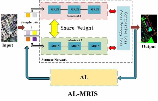
  • An active learning-based multipath residual involution Siamese network for few-shot HSI classification, AL-MRIS, is proposed. In the AL-MRIS method, the multipath residual involution (MRIN) module can comprehensively consider the local features, dynamic features and global features of HSIs. Moreover, to address the sample scarcity problem, the AL strategy is integrated into the Siamese network to make the training samples more representative to improve the classification performance.
  • An AL-based Siamese network framework is constructed. The Siamese network can extract information beyond labels from the data itself, thereby achieving better classification performance, especially for few-shot training samples. Moreover, by integrating with AL, representative samples can be selected more effectively, thus improving the ability of the Siamese network to discriminate features while reducing the practical labeling cost.
  • The multipath residual involution (MRIN) module is proposed. The MRIN module captures fine-grained features via an involution operation and effectively aggregates the contextual semantic information of the HSI through dynamic weights. Moreover, the MRIN module comprehensively considers local features, dynamic features and global features through multipath residual connections, which improves the representation ability of HSIs.
  • A cosine distance-based contrastive loss (CD loss) for Siamese networks is proposed. The CD loss utilizes the directional similarity of high-dimensional HSI data and improves the discriminability of the Siamese classification network.
The remainder of this paper is organized as follows: Section 2 provides a brief introduction to related technologies. Section 3 provides a detailed description of our proposed AL-MRIS method and its internal modules. Section 4 shows the classification results, and several key parameters are discussed and analyzed. Finally, Section 5 provides the conclusion.

2. Related Works

This section provides a brief overview of related work, including two key technologies: the involution network and the Siamese network.

2.1. Involution Network

An involution network is a kind of deep learning network that was proposed by Duo Li et al. in 2021 [28] to improve flexibility when processing spatial information. Compared with traditional CNNs, the involution network proposes a new operation called the ‘involution’. At its core is the ‘involution’ layer, which replaces traditional convolution operations with local interactions of adaptive weights.
The traditional convolution operation is based on the convolution kernel to extract element-by-element products from the input image and sum the product results to obtain the output. However, this approach limits the ability of the convolution kernel to adapt to diverse visual patterns according to different spatial locations, and the convolution receptive field is also locally limited, preventing it from handling small objects and blurred images well. In addition, traditional convolutional filters exhibit redundancy, which affects the flexibility of the convolutional kernel. In contrast, in the ‘involution’ operation, the network computation is neatly divided into two parts: ‘kernel generation’ and ‘Multiply–Add’. This operation obviously reduces the number of parameters and computations, thus improving the efficiency of the network. Compared with traditional convolutional operations, involution operations have ‘spatial-specific’ and ‘channel-agnostic’ characteristics; these operations can adaptively assign weights to different positions and prioritize the visual elements with the most information in the spatial domain.
The involution operator is a nonlinear transformation method that utilizes a learnable weight matrix to process the feature. Its uniqueness lies in the dynamism of the weight matrix, which can be adjusted according to the input feature. This dynamic adjustment enables the involution operator to better adapt to different types of features and improve the effectiveness of feature extraction. The involution kernel is a trainable matrix that multiplies the features element by element and then adds the results element by element to generate the output feature.
As shown in Figure 1, let X I n v R H × W × C represent the input feature, where H   a n d   W represent its height and width, respectively, and C represents the input channel. Within the cuboid of the input feature tensor X I n v , the feature vector ( X I n v ) i , j R C represents the pixel located at position ( i , j ) . The output of the involution operation Y I n v can be defined by the following Formula (1):
Y I n v i , j , k = u , v Δ K H i , j , u + K 2 , v + K 2 , k G C ( X I n v ) i + u , j + v , k ,
where H R H × W × K × K × G is an involution kernel and H i , j , , , g R K × K , g = 1,2 , , G . G is the number of groups sharing the same involution kernel. Δ K is the set of neighborhood offsets convolved over the central pixel, represented as the Cartesian product, as shown in Formula (2):
Δ K = K 2 , , K 2 × K 2 , , K 2 .
The shape of the involution kernels H depends on the shape of the input feature X I n v . The kernel generation function is denoted as ϕ , and the kernel generation at each ( i , j ) position is calculated via Formula (3):
H i , j = ϕ ( X I n v ) Ψ i , j ,
Ψ i , j represents the index of the pixel set H i , j . Formally, there is a kernel generation function ϕ : R C R K × K × G , which is specifically defined as Formula (4):
H i , j = ϕ ( X I n v ) i , j = ω 1 σ ω 0 ( X I n v ) i , j ,
Here, ω 0 R C r × C   a n d   ω 1 R K × K × G × C r represent two linear transformations, which together form a bottleneck layer. σ denotes batch normalization and a nonlinear activation function.

2.2. Siamese Network

The core of the Siamese network structure is to map input sample pairs to the same feature space through two subnetworks, and the two subnetworks have shared weights. This allows the network to learn a common representation that makes similar inputs closer in the feature space [20]. The Siamese network is usually used for dealing with the problem of measurement learning and similarity comparison. Two inputs in the sample pairs are passed through the shared weights subnetworks. Then, representations of the two vectors are obtained, and the similarity score is calculated between these two vector representations. This score can be used to indicate the similarity degree of two inputs, as shown in Figure 2. The Siamese network usually uses a contrast loss function to analyze the similarity scores of two input samples. By adjusting the network parameters, the similarity scores of similar input pairs increase, and the similarity scores of dissimilar input pairs decrease, thus improving the classification accuracy of the model. During the training stage, rather than directly classifying input samples, the Siamese network evaluates the similarities between input samples through learning, which enables it to learn representations of input data effectively without requiring a large number of labeled samples. In practical applications, the Siamese network is widely used in face verification [30], signature verification [31], target tracking [32] and other fields.

3. Our Proposed AL-MRIS Method

For few-shot HSI classification, an AL-based multipath residual involution Siamese network, named AL-MRIS, was proposed. The flowchart of the AL-MRIS method is shown in Figure 3. The multipath residual involution (MRIN) module comprehensively considers the local, dynamic and global features in HSIs. Moreover, to solve the sample scarcity problem, by integrating the Siamese network with AL, representative samples can be selected more effectively, thus improving the discriminative ability of the Siamese network while reducing the practical labeling cost.

3.1. The Multipath Residual Involution (MRIN) Module

To make full use of the rich features in HSIs, inspired by [28], a multipath residual involution (MRIN) module was proposed. The MRIN module adopts an involution operation to capture fine-grained features and effectively aggregates the contextual semantic information of HSIs through dynamic weights. Moreover, the MRIN module comprehensively considers local features, dynamic features and global features through multipath residual connections, which improves the representation ability of HSIs. A specific block diagram of the MRIN module is shown in Figure 4.
In the proposed MRIN module, there are three branches: a local feature branch, a dynamic feature branch and a global feature branch. The middle gray arrow branch is the dynamic feature branch, which extracts the core dynamic spectral–spatial feature via an involution operation. Through an involution operation, the adaptive convolution kernel can dynamically adjust weights within the receptive field to adapt to different spatial structures in HSIs. This approach expands the spatial range of utilized images, effectively aggregates the contextual semantic information in HSIs, and effectively extracts HSI features in nonuniform and complex spaces. The involution operation enhances the representation by using nonlinear transformations through nonlinear activation functions and has advantages in processing irregular shape regions and local structural information from HSIs. The involution operation is followed by a 1 × 1 Conv operation to maintain channel consistency. The upper purple arrow branch is the local feature branch, which uses a 3 × 3 Conv operation to extract local spatial features. At the same time, the lower yellow arrow branch is the global feature branch, which directly uses skip connections to transmit the information of the front layer and fuse the global features. The three branches are connected through a residual addition operation. The multipath residual connection not only helps the network maintain the integrity of information between different layers but also integrates different features to enhance the representation ability of the model. In addition, this approach accelerates convergence, alleviates the problem of gradient disappearance or gradient explosion and can be applied to deeper network structures.
Assuming that X R H × W × C represents the input feature of the MRIN module, the output of the MRIN module CIN(X) can be represented by the following Formula (5):
C I N X = σ C o n v 1 × 1 I n v X + σ C o n v 3 × 3 X + X ,
σ · indicates the batch normalization and activation functions, Conv1 × 1(∙) represents a 2D convolution with a kernel size of 1 × 1 to maintain channel consistency and Conv3 × 3(∙) represents a 2D convolution with a kernel size of 3 × 3.
To achieve better feature aggregation, the proposed AL-MRIS network concatenates MRIN modules three times in series, and the concatenated module output Ը can be represented by the following Formula (6):
Ը = C I N t r i X = C I N C I N C I N X .

3.2. AL-Based Siamese Network

According to practical conditions, the acquisition of real hyperspectral labeled samples is time consuming, labor intensive and costly, and an AL-based Siamese network framework is proposed for few-shot HSI classification. The Siamese network can extract information beyond labels from the data itself, thereby achieving better classification performance. To a certain extent, the construction of sample pairs in the Siamese network can achieve data augmentation and alleviate the overfitting problem in the network training process. Moreover, by integrating with AL, representative samples can be selected more effectively, thus improving the ability of the Siamese network to discriminate features while reducing the practical labeling cost. In summary, as shown in Figure 5, the AL-based Siamese network framework includes three main steps: Siamese network learning using the training sample set, AL selecting newly labeled training samples and updating the training set.

3.2.1. Construct Sample Pairs Based on the Training Sample Set

Initially, one sample from each class is randomly selected to constitute the training set S e t o r i _ L a b l e . Considering the spatial information of the HSI, the training set includes N C c l a s s R H × W × C labeled 3D data blocks. Each block consists of the central labeled pixel and its surrounding neighborhood pixels, denoted as X = { x 1 , x 2 , , x N C c l a s s } . The labels corresponding to these data blocks are represented by the set Y = Y 1 , Y 2 , , Y s , , Y N C c l a s s , where Y s { 1,2 , , N C c l a s s } and N C c l a s s is the total number of classes in the HSI. The inputs of the proposed AL-MRIS algorithm are sample pairs, and a set of sample pairs S e t p a i r s is constructed by traversing all possible combinations in S e t o r i _ L a b l e , achieving data augmentation to a certain extent. The sample pairs in S e t p a i r s are denoted as X n , X m , and their corresponding labels are given in Formula (7):
Y n , m = L a b e l X n , X m = 1                     i f   Y n = Y m 0                     i f   Y n Y m .
The sample pair label Y n , m represents whether the classes of the sample pair are consistent.

3.2.2. Siamese Network Learning Using the Training Set

The two samples in the training pair X n , X m are separately input into the two subnetworks of AL-MRIS through learning to deeply mine the rich information inherent in the samples themselves and decreasing the interclass distance and intraclass distance. The subnetworks of the AL-MRIS are mainly composed of three serially connected MRIN modules. The input X is passed through three serial MRIN modules to obtain the output Ը . Then, Ը is passed through the C o v _ s p e · operation and combined with itself by residual connection to obtain the advanced feature output Թ ( X ) , as represented in Formula (8):
Թ X = C o v _ s p e ( C o v _ s p e ( Ը ) + Ը ) ,
C o v _ s p e · includes a 7 × 1 × 1 convolutional layer, a batch normalization layer and a Relu activation layer.
The subnetwork of AL-MRIS learns advanced features Թ X from the input patch X, with a simple network structure and high learning efficiency. Next, adaptive average pooling operations are utilized to extract 1 × 1 × 96 feature vectors from Թ X , a fully connected layer is used to transform them into a prediction vector f X with a size of 1 × C and the preliminary training by using the initial training set is completed, which can be represented by the following Formula (9):
f X = L i n e a r A v g P o o l 2 d Թ X ,
A v g P o o l 2 d · represents the adaptive average pooling operation, and L i n e a r · represents the fully connected layer.
During the contrastive learning process, the parameter θ was used to update the model. The updating θ processes are shown in Formulas (10)–(13):
θ = a r g m i n L c o n t r a f X n , f X m , Y n , m ; θ .
For HSI classification, a cosine distance-based contrastive loss (CD loss) for Siamese networks was proposed to minimize the intraclass distance and maximize the interclass distance.
The CD loss utilizes the directional similarity of high-dimensional HSI data and improves the discriminability of the Siamese classification network. It can be represented by the following Formula (11):
L c o n t r a = 1 2 Y n , m d 2 + 1 Y n , m max m a r g i n d , 0 2 ,
where the margin is a constant value set to 1.25, which is used to maintain the lower bound of the distance between negative sample pairs. d represents the cosine distance between the feature vectors of sample pairs f X n and f X m and can be expressed by Formula (12):
d = f X n f X m m a x f X n 2 , ϵ m a x f X m 2 2 , ϵ ,
ϵ is a constant 1 × 10 8 and is a small value to avoid zero division errors.
The cosine distance metric enhances the network model’s sensitivity to the direction similarity for HSIs rather than simply focusing on the numerical magnitude. The goal is to minimize the contrastive loss function L c o n t r a by optimizing the parameters θ so that the model can bring similar samples closer in the representation space while pushing away dissimilar samples. The cosine distance effectively anchors the learning focus of the Siamese network, ensuring directional similarity rather than absolute feature value differences as the basis for discrimination, thus forming meaningful and distinctive mapping in the representation space.
In the classification learning process, the class label with the highest predicted probability value is selected as the predicted label Y. This label can be represented by Formula (13):
Y = f q X m a x , q 1,2 , , N C c l a s s .
The cross-entropy loss was used for retraining θ . First, we define the cross-entropy loss function L c r o s s e n t r o p y , which is used to measure the distance between the predicted labels and the real labels. The cross-entropy loss function is shown in Formula (14):
L c r o s s e n t r o p y = i = 1 N Y q × l o g Y ^ q ,
where Y q is the real label of the q -th sample and Y ^ i is the predicted label of the q -th sample. Next, the parameter θ is used to update the model to decrease the value of the cross-entropy loss function. The update process is shown in Formula (15):
θ = a r g m i n L c r o s s e n t r o p y f X q , Y q ; θ .
X q and Y q represent the q -th training sample and its label, respectively.

3.2.3. AL Selecting Newly Labeled Training Samples

After the training of the Siamese network, the remaining unlabeled sample is input into the model to obtain the classification prediction probability P p r e d i c t i o n . Then, for each class, the sample with the highest prediction probability is selected, and manual annotation is used to obtain the corresponding real label. It can be represented by the following Formula (16):
P p r e d i c t i o n = max f X u n l a b l e d = p 1 , m a x , p 2 , m a x , , p t , m a x , , p c , m a x ,
p t , m a x denotes the sample with the maximum predicted probability value in class t . Then, through manual annotation, the real label P t r u e can be obtained as Formula (17):
P t r u e = M a n u a l P p r e d i c t i o n .
The AL stage can select representative samples more effectively, thus improving the ability of the Siamese network to discriminate features while reducing the practical labeling cost.

3.2.4. Updating the Training Set

The newly labeled samples S e t n e w _ L a b l e are added to the original training set S e t o r i _ L a b l e to update the training sample set, which can be represented by the following Formula (18):
S e t o r i _ L a b l e = S e t o r i _ L a b l e S e t n e w _ L a b l e .
The whole network is updated using the latest training sample set data, and continuous iterative optimization is performed. The updated network is used for the next round of uncertainty evaluation and sample selection. Through continuous iteration, the training sample set gradually expands, and the classification performance of the network is also enhanced. After the training sample set expands to a certain size, the whole network parameters are fixed, and then the unlabeled samples are passed through the network to obtain the final classification result.

4. Experiments and Results

In this section, three real HSI datasets were used to validate the classification performance of the proposed network. For each dataset, initially, one sample from each class is randomly selected to constitute the training set, and in every round, the AL stage selects one more sample from each class to add to the training set. Eventually, three samples from each class were included in the final training set, and ten repeated experiments were conducted, with the average value serving as the final experimental result. The proposed AL-MRIS utilized a sliding window of 11 × 11 size to generate a series of data blocks. In the contrastive learning process, the learning rate and the weight decay parameter were set to 5 × 10 5 and 0, respectively. During the classification process, the learning rate and the weight decay parameter were set to 1 × 10 3 and 5 × 10 5 , respectively. All the experiments were carried out on a server equipped with 80 GB of memory and an RTX 3080 GPU and were implemented in Python.

4.1. Datasets

The University of Pavia (PU) dataset was captured in an urban scene in the city of Pavia using the ROSIS (Reflective Optics System Imaging Spectrometer) sensor. The spatial resolution is 1.3 m. The dataset contains spectral wavelengths ranging from 430 to 860 nanometers. The dataset has a size of 610 × 340 pixels and 103 spectral bands. The PU dataset included 9 different land cover classes, and the names of these classes and the number of samples are shown in Table 1. Additionally, Figure 6 presents the pseudocolor image and the corresponding ground truth image to more intuitively showcase the characteristics of the PU dataset.
The Indian Pines (IP) dataset was collected by the Airborne Visible/Infrared Imaging Spectrometer (AVIRIS) sensor over the IP area in northwestern Indiana in 1996 with a spatial resolution of 20 m. This dataset contains one of the earliest HSI datasets. The dataset included 220 bands, after which the noisy and water absorption bands were removed; the remaining 200 bands (consisting of bands 1 to 103, 109 to 149 and 164 to 219) were used for the experiments. The IP dataset has a size of 145 × 145 pixels. In the data scene, sixteen different classes are covered. The detailed class names and sample quantities can be found in Table 2. In addition, Figure 7 shows the pseudocolor image of the IP dataset and the corresponding ground truth image.
The Salinas Valley (SA) dataset was captured by the AVIRIS sensor in the Salinas Valley area of California, United States, in 1998. The spatial resolution is 3.7 m. The dataset was stripped of 20 water absorption bands, leaving 144 usable bands. The size of the SA dataset is 512 × 217 pixels. In the data scene, 16 different classes are covered. Table 3 provides detailed information on the names and numbers of samples for each class, and Figure 8 shows the pseudocolor image and ground truth image.

4.2. Evaluation Metrics

Three common classification metrics were used to evaluate the classification performance: overall accuracy (OA) [33], average accuracy (AA) [34] and Kappa coefficient (Kappa) [33]. OA represents the proportion of correctly classified labels to the total number of labels. AA is the mean value of the classification accuracies for all the classes, while Kappa measures the agreement between the predicted labels and the real labels. By using these metrics, the classification performance can be evaluated more comprehensively.

4.3. Comparison of Different Classification Methods

To further verify the effectiveness of the proposed AL-MRIS method, several state-of-the-art classification methods, including DRIN [29], 3DCSN [20], S3Net [23], ALPN [26], FAAL [27], CFSL [16] and Gia-CFSL [17], were used for comparison. The corresponding classification maps are shown in Figure 9, Figure 10, Figure 11 and Figure 12. Compared with the classification maps of the other methods, the classification map obtained by the proposed AL-MRIS method is closest to the ground truth map. The corresponding classification accuracy results are shown in Table 4, Table 5 and Table 6. The proposed AL-MRIS method achieves optimal OA, AA and Kappa results on all three datasets. For the PU dataset, the OA of the proposed AL-MRIS method reaches 84.71%; this value is 5.34% higher than that of the CFSL method (79.37%), which has the highest accuracy among the comparison methods, and 47.53% higher than that of the FAAL method (37.18%). For the IP dataset, the OA of the AL-MRIS method reached 75.31%, which was 6.84% higher than that of the CFSL method (68.47%), which has the highest accuracy among the comparison methods. Compared with that of FAAL (32.42%), the OA of the AL-MRIS method was 42.89% higher. For the SA dataset, the OA of the AL-MRIS method was 90.18%, which was 1.34% higher than that of S3Net (88.84%) and 27.61% higher than that of FAAL (62.57%). Meanwhile, Table 4 shows that for the PU dataset the proposed AL-MRIS method achieves the highest classification accuracy in Asphalt, Meadows, Painted metal sheets, and Bare Soil. Figure 10 shows the partial enlarged PU classification maps, and Asphalt (in red) and Meadows (in light green) in the AL-MRIS classification map are the closest to the ground truth distribution.
The reasons that the proposed AL-MRIS method can achieve the best classification effect are as follows: The MRIN module in proposed AL-MRIS method can comprehensively consider the local features, dynamic features and global features through the multipath residual connection, which improve the representation ability of HSI. Moreover, by integrating the Siamese network with AL, representative samples can be selected more effectively, thus improving the ability of the Siamese network to discriminate. Moreover, the CD loss utilized the directional similarity of high-dimensional HSI data, and the discriminability of the Siamese classification network improved.

4.4. Parameter Discussions

This section discusses and analyzes the key parameters of the proposed AL-MRIS method. The PU dataset was used for analysis. Initially, one sample from each class was randomly selected, and despite being at the AL stage, three samples from each class were ultimately included in the final training set.

4.4.1. Impacts of the MRIN Module Number

To analyze the impacts of the MRIN module number, the number of concatenated MRIN modules was set to 1, 2, 3, 4 and 5; the classification results are shown in Figure 13. When the concatenation number is three, the OA, AA and Kappa all yield optimal performances.
The reasons for this difference are as follows: when the concatenation number is one, only a single MRIN module is used, and the features of the input image are not fully mined, leading to the lowest classification results. When the concatenated number is more than one, the classification performance is improved because the concatenated modules can obtain more rich and complex comprehensive information by gradually extracting and combining the features. However, when the concatenation number is too large, the gradient is easily diluted or amplified during backpropagation, leading to difficulties or degradation in network training. Therefore, as shown in Figure 13, when the concatenation number is 3, the network can make full use of image features while avoiding the problem of gradient disappearance or gradient explosion, thus achieving the best classification performance. According to the results and the analysis, to achieve better feature aggregation, the proposed AL-MRIS network concatenates MRIN modules three times in series.

4.4.2. Comparison of Different Distance-Based Contrast Losses

To verify the advantages of the proposed cosine distance-based contrastive loss (CD loss), comparison experiments with three other distance-based contrast loss functions (European distance-based contrast loss, Minkowski-based contrast loss and Jensen–Shannon-based contrast loss) were conducted. The classification accuracy results for different distance-based contrast losses are listed in Table 7. As shown in Table 7, the classification results of the proposed CD loss are higher than those of any other comparison loss for OA, AA and Kappa. The OA of the CD loss was 84.71%, which was 1.94% higher than that of the European distance-based contrast loss (82.77%). This loss was 4.64% higher than the Minkowski-based contrast loss (80.07%) and 5.4% higher than the Jensen–Shannon-based contrast loss (79.31%). Moreover, for a more intuitive presentation, Figure 14 displays an intuitive comparison of OA.
The reason why the CD loss can achieve the best classification performance is that the cosine distance enhances the network model’s sensitivity to the direction similarity for HSIs rather than simply focusing on the numerical magnitude. For high-dimensional HSI data, the direction can better capture the similarity than the distance. Therefore, the CD loss improves the discriminability of the Siamese classification network.

4.4.3. Influences of Different Training Sample Numbers

This section discusses the influences of different training sample numbers on the classification methods. In the PU dataset, two, three four, five and six labeled samples were used as training samples, and the proposed AL-MRIS method was compared with four representative methods: 3DCSN, ALPN, DRIN and Gia-CFSL. The OA results for the classification methods with different training samples are shown in Figure 15. The classification performances of all the classification methods gradually improve with the increasing training sample number because as the number of training samples increases, more information becomes available for the classification process. Moreover, the proposed AL-MRIS method outperforms all the comparison methods for different training sample numbers and achieves the highest OA, which indicates that the proposed AL-MRIS method has excellent classification performance and is especially suitable for few-shot classification.

4.4.4. Ablation Experiments

To verify the validity of the Siamese network framework, AL strategy and MRIN module in the proposed AL-MRIS method, ablation experiments were carried out on the PU dataset, and the classification results are shown in Table 8. As shown in Table 8, compared with those of the proposed AL-MRIS method, when the Siamese network framework was missing, the OA decreased by 17.99%, the AA decreased by 20.12% and the Kappa decreased by 22.40%. This is because the Siamese network framework achieves data augmentation to a certain extent and can extract information beyond labels from the data itself, thereby achieving better classification performance. Through learning, the Siamese network explore the rich information inherent in the samples themselves and decreases the interclass distance and decreases intraclass distance. When the AL strategy was abandoned, the OA decreased by 10.20%, the AA decreased by 9.26%, and the Kappa decreased by 10.99%. This shows that through the AL strategy, representative samples can be selected more effectively, thus improving the network’s discriminant ability. When the MIRN module was replaced with a normal 3D convolution, the OA decreased by 20.29%, the AA decreased by 31.41%, and the Kappa decreased by 27.30%. This finding verifies that the MIRN module comprehensively considers local features, dynamic features and global features, which improves the representation ability of HSIs.

5. Conclusions

For few-shot HSI classification, an active learning (AL)-based multipath residual involution Siamese network, named AL-MRIS, is proposed. In the AL-MRIN method, an AL-based Siamese network framework is constructed, and representative samples can be selected more effectively, thus improving the discriminative ability of the Siamese network. An MRIN module is designed to comprehensively consider local features, dynamic features and global features, which improves the representation ability of HSIs. Moreover, a CD loss function for Siamese networks is proposed to utilize the directional similarity of high-dimensional HSI data, and this approach improves the discriminability of the Siamese classification network. A large number of experimental results show that the proposed AL-MRIS method can achieve excellent classification performance with only a few training samples. Moreover, for few-shot HSI classification, we will try to integrate AL-MRIN with cross-domain learning in the future to further improve the classification performance.

Author Contributions

Conceptualization, J.Y. and J.Q. (Jia Qin); Methodology, J.Y. and J.Q. (Jia Qin); Original draft preparation, J.Q. (Jia Qin); Review and editing, J.Y., J.Q. (Jinxi Qian) and A.L.; Valuable advice, J.Q. (Jinxi Qian) and L.W. All authors have read and agreed to the published version of the manuscript.

Funding

This research was funded by the National Natural Science Foundation of China (Nos. 62001434, 62071084).

Data Availability Statement

The three real HSI datasets analyzed during the research can be found at http://www.ehu.eus/ccwintco/index.php/Hyperspectral_Remote_Sensing_Scenes, which was accessed on 1 May 2023.

Acknowledgments

The authors wish to express gratitude for the valuable comments and suggestions provided by the editors and the anonymous reviewers.

Conflicts of Interest

The authors declare no conflict of interest.

References

  1. Janne, M.; Sarita, K.-S.; Sonja, K.; Topi, T.; Pekka, H.; Peter, K.; Laura, P.; Arto, V.; Sakari, T.; Timo, K.; et al. Tree species classification from airborne hyperspectral and LiDAR data using 3D convolutional neural networks. Remote Sens. Environ. Interdiscip. J. 2021, 256, 112322. [Google Scholar]
  2. Teng, M.Y.; Mehrubeoglu, R.; King, S.A.; Cammarata, K.; Simons, J. Investigation of epifauna coverage on seagrass blades using spatial and spectral analysis of hyperspectral images. In Proceedings of the 2013 5th Workshop on Hyperspectral Image and Signal Processing: Evolution in Remote Sensing (WHISPERS), Gainesville, FL, USA, 26–28 June 2013. [Google Scholar] [CrossRef]
  3. Kirsch, M.; Lorenz, S.; Zimmermann, R.; Tusa, L.; Möckel, R.; Hödl, P.; Booysen, R.; Khodadadzadeh, M.; Gloaguen, R. Integration of Terrestrial and Drone-Borne Hyperspectral and Photogrammetric Sensing Methods for Exploration Mapping and Mining Monitoring. Remote Sens. 2018, 10, 1366. [Google Scholar] [CrossRef]
  4. Roy, S.K.; Krishna, G.; Dubey, S.R.; Chaudhuri, B.B. HybridSN: Exploring 3-D–2-D CNN Feature Hierarchy for Hyperspectral Image Classification. IEEE Geosci. Remote Sens. Lett. 2020, 17, 277–281. [Google Scholar] [CrossRef]
  5. Tao, H.; Duan, Q.; Lu, M.; Hu, Z. Learning discriminative feature representation with pixel-level supervision for forest smoke recognition. Pattern Recognit. J. Pattern Recognit. Soc. 2023, 143, 109761. [Google Scholar] [CrossRef]
  6. Deng, B.; Jia, S.; Shi, D. Deep Metric Learning-Based Feature Embedding for Hyperspectral Image Classification. IEEE Trans. Geosci. Remote Sens. 2019, 58, 1422–1435. [Google Scholar] [CrossRef]
  7. Guo, A.J.X.; Zhu, F. A CNN-Based Spatial Feature Fusion Algorithm for Hyperspectral Imagery Classification. IEEE Trans. Geosci. Remote Sens. 2019, 57, 7170–7181. [Google Scholar] [CrossRef]
  8. Gao, K.; Liu, B.; Yu, X.; Zhang, P.; Tan, X.; Sun, Y. Small sample classification of hyperspectral image using model-agnostic meta-learning algorithm and convolutional neural network. Int. J. Remote Sens. 2021, 42, 3090–3122. [Google Scholar] [CrossRef]
  9. Li, W.; Liu, Q.; Zhang, Y.; Wang, Y.; Yuan, Y.; Jia, Y.; He, Y. Few-Shot Hyperspectral Image Classification Using Meta Learning and Regularized Finetuning. IEEE Trans. Geosci. Remote Sens. 2023, 61, 1–14. [Google Scholar] [CrossRef]
  10. Zhang, J.; Liu, L.; Zhao, R.; Shi, Z. A Bayesian Meta-Learning-Based Method for Few-Shot Hyperspectral Image Classification. IEEE Trans. Geosci. Remote Sens. 2023, 61, 5500613. [Google Scholar] [CrossRef]
  11. Cao, M.; Zhao, G.; Dong, A.; Lv, G.; Guo, Y.; Dong, X. Few-Shot Hyperspectral Image Classification Based on Cross-Domain Spectral Semantic Relation Transformer. In Proceedings of the 2023 IEEE International Conference on Image Processing (ICIP), Kuala Lumpur, Malaysia, 9–12 October 2023; pp. 1375–1379. [Google Scholar]
  12. Li, Z.; Liu, M.; Chen, Y.; Xu, Y.; Li, W.; Du, Q. Deep Cross-Domain Few-Shot Learning for Hyperspectral Image Classification. IEEE Trans. Geosci. Remote Sens. 2021, 60, 5501618. [Google Scholar] [CrossRef]
  13. Zhang, C.; Zhong, S.; Gong, C. Feature Integration-Based Training for Cross-Domain Hyperspectral Image Classification. In Proceedings of the IGARSS 2022—2022 IEEE International Geoscience and Remote Sensing Symposium, Kuala Lumpur, Malaysia, 17–22 July 2022; pp. 3572–3575. [Google Scholar]
  14. Wang, B.; Xu, Y.; Wu, Z.; Zhan, T.; Wei, Z. Spatial–Spectral Local Domain Adaption for Cross Domain Few Shot Hyperspectral Images Classification. IEEE Trans. Geosci. Remote Sens. 2022, 60, 5539515. [Google Scholar] [CrossRef]
  15. Wang, W.; Liu, F.; Liu, J.; Xiao, L. Cross-Domain Few-Shot Hyperspectral Image Classification with Class-Wise Attention. IEEE Trans. Geosci. Remote Sens. 2023, 61, 5502418. [Google Scholar] [CrossRef]
  16. Huang, K.-K.; Yuan, H.T.; Ren, C.X.; Hou, Y.E.; Duan, J.L.; Yang, Z. Hyperspectral Image Classification via Cross-Domain Few-Shot Learning with Kernel Triplet Loss. IEEE Trans. Geosci. Remote Sens. 2023, 61, 5530818. [Google Scholar] [CrossRef]
  17. Zhang, Y.; Li, W.; Zhang, M.; Wang, S.; Tao, R.; Du, Q. Graph Information Aggregation Cross-Domain Few-Shot Learning for Hyperspectral Image Classification. IEEE Trans. Neural Netw. Learn. Syst. 2022, 35, 1912–1925. [Google Scholar] [CrossRef]
  18. Li, Z.; Guo, H.; Chen, Y.; Liu, C.; Du, Q.; Fang, Z. Few-Shot Hyperspectral Image Classification with Self-Supervised Learning. IEEE Trans. Geosci. Remote Sens. 2023, 61, 5517917. [Google Scholar] [CrossRef]
  19. Li, Y.; Zhang, L.; Wei, W.; Zhang, Y. Deep Self-Supervised Learning for Few-Shot Hyperspectral Image Classification. In Proceedings of the IGARSS 2020—2020 IEEE International Geoscience and Remote Sensing Symposium, Waikoloa, HI, USA, 26 September–2 October 2020; pp. 501–504. [Google Scholar]
  20. Cao, Z.; Li, X.; Jiang, J.; Zhao, L. 3D convolutional Siamese network for few-shot hyperspectral classification. J. Appl. Remote Sens. 2020, 14, 048504. [Google Scholar] [CrossRef]
  21. Huang, L.; Chen, Y. Dual-Path Siamese CNN for Hyperspectral Image Classification with Limited Training Samples. IEEE Geosci. Remote Sens. Lett. 2024, 18, 518–522. [Google Scholar] [CrossRef]
  22. Wang, W.; Chen, Y.; He, X.; Li, Z. Soft Augmentation-Based Siamese CNN for Hyperspectral Image Classification with Limited Training Samples. IEEE Geosci. Remote Sens. Lett. 2022, 19, 5508505. [Google Scholar] [CrossRef]
  23. Xue, Z.; Zhou, Y.; Du, P. S3Net: Spectral–Spatial Siamese Network for Few-Shot Hyperspectral Image Classification. IEEE Trans. Geosci. Remote Sens. 2022, 60, 5531219. [Google Scholar] [CrossRef]
  24. Hou, W.; Chen, N.; Peng, J.; Sun, W. A Prototype and Active Learning Network for Small-Sample Hyperspectral Image Classification. IEEE Geosci. Remote Sens. Lett. 2023, 20, 5510805. [Google Scholar] [CrossRef]
  25. Ma, K.Y.; Chang, C.-I. Iterative Training Sampling Coupled with Active Learning for Semi supervised Spectral–Spatial Hyperspectral Image Classification. IEEE Trans. Geosci. Remote Sens. 2021, 59, 8672–8692. [Google Scholar] [CrossRef]
  26. Li, X.; Cao, Z.; Zhao, L.; Jiang, J. ALPN: Active-Learning-Based Prototypical Network for Few-Shot Hyperspectral Imagery Classification. IEEE Geosci. Remote Sens. Lett. 2022, 19, 5508305. [Google Scholar] [CrossRef]
  27. Wang, G.; Ren, P. Hyperspectral Image Classification with Feature-Oriented Adversarial Active Learning. Remote Sens. 2020, 12, 3879. [Google Scholar] [CrossRef]
  28. Li, D.; Hu, J.; Wang, C.; Li, X.; She, Q.; Zhu, L.; Zhang, T.; Chen, Q. Involution: Inverting the Inherence of Convolution for Visual Recognition. arXiv 2021. [Google Scholar] [CrossRef]
  29. Meng, Z.; Zhao, F.; Liang, M.; Xie, W. Deep Residual Involution Network for Hyperspectral Image Classification. Remote Sens. 2021, 13, 3055. [Google Scholar] [CrossRef]
  30. Wu, H.; Xu, Z.; Zhang, J.; Yan, W.; Ma, X. Face recognition based on convolution siamese networks. In Proceedings of the 2017 10th International Congress on Image and Signal Processing, BioMedical Engineering and Informatics (CISP-BMEI), Shanghai, China, 14–16 October 2017; IEEE: Piscataway, NJ, USA, 2018. [Google Scholar] [CrossRef]
  31. Dey, S.; Dutta, A.; Toledo, J.I.; Ghosh, S.K.; Llados, J.; Pal, U. SigNet: Convolutional Siamese Network for Writer Independent Offline Signature Verification. arXiv 2017. [Google Scholar] [CrossRef]
  32. Chen, Z.; Zhong, B.; Li, G.; Zhang, S.; Ji, R. Siamese Box Adaptive Network for Visual Tracking. In Proceedings of the IEEE/CVF conference on computer vision and pattern recognition, Seattle, WA, USA, 13–19 June 2020. [Google Scholar] [CrossRef]
  33. Foody, G.M. Status of land cover classification accuracy assessment. Remote Sens. Environ. 2002, 80, 185–201. [Google Scholar] [CrossRef]
  34. Richards, J.A. Classifier performance and map accuracy. Remote Sens. Environ. 1996, 57, 161–166. [Google Scholar] [CrossRef]
Figure 1. Schematic diagram of involution. The input is H i , j , and the output is Y I n v .
Remotesensing 16 00990 g001
Figure 2. Siamese network structure.
Remotesensing 16 00990 g002
Figure 3. Flowchart of AL-MRIN. The red and green regions represent the two Siamese subnetworks, and the blue regions represent the active learning strategy.
Remotesensing 16 00990 g003
Figure 4. Diagram of the MRIN module. The middle gray arrow branch is a dynamic feature branch, the upper purple arrow branch is a local feature branch and the lower yellow arrow branch is a global feature branch.
Remotesensing 16 00990 g004
Figure 5. The framework of the AL-based Siamese network.
Remotesensing 16 00990 g005
Figure 6. The pseudocolor image and ground truth image of the PU dataset. (a) The pseudocolor image. (b) The ground truth image.
Remotesensing 16 00990 g006
Figure 7. The pseudocolor image and ground truth image of the IP dataset. (a) The pseudocolor image. (b) The ground truth image.
Remotesensing 16 00990 g007
Figure 8. The pseudocolor image and ground truth image of the SA dataset. (a) The pseudocolor image. (b) The ground truth image.
Remotesensing 16 00990 g008
Figure 9. Classification maps of the PU dataset: (a) Ground truth, (b) DRIN, (c) Sia-3DCNN, (d) 3DCSN, (e) S3Net, (f) ALPN, (g) FAAL, (h) CFSL, (i) Gia-CFSL and (j) Proposed AL-MRIS.
Remotesensing 16 00990 g009
Figure 10. Partial enlarged classification maps obtained for the PU dataset: (a) ground truth, (b) DRIN, (c) Sia-3DCNN, (d) 3DCSN, (e) S3Net, (f) ALPN, (g) FAAL, (h) CFSL, (i) Gia-CFSL, and (j) proposed AL-MRIS.
Remotesensing 16 00990 g010
Figure 11. Classification maps of the IP dataset: (a) ground truth, (b) DRIN, (c) Sia-3DCNN, (d) 3DCSN, (e) S3Net, (f) ALPN, (g) FAAL, (h) CFSL, (i) Gia-CFSL and (j) proposed AL-MRIS.
Remotesensing 16 00990 g011
Figure 12. Classification maps of the SA dataset: (a) ground truth, (b) DRIN, (c) Sia-3DCNN, (d) 3DCSN, (e) S3Net, (f) ALPN, (g) FAAL, (h) CFSL, (i) Gia-CFSL and (j) proposed AL-MRIS.
Remotesensing 16 00990 g012
Figure 13. Classification results for different numbers of MRIN modules.
Remotesensing 16 00990 g013
Figure 14. OA results for different distance-based contrast losses.
Remotesensing 16 00990 g014
Figure 15. OA results with different training sample numbers.
Remotesensing 16 00990 g015
Table 1. The number of sample classes in the PU dataset.
LabelClass#Number
1Asphalt6631
2Meadows18,649
3Gravel2099
4Trees3064
5Painted metal sheets1345
6Bare Soil5029
7Bitumen1330
8Self-Blocking Bricks3682
9Shadows947
Total (9 classes)42,776
Table 2. The number of sample classes in the IP dataset.
LabelClass#Number
1Alfalfa40
2Corn–notill1428
3Corn–mintill830
4Corn237
5Grass–pasture483
6Grass–trees730
7Grass–pasture–mowed28
8Hay–windrowed478
9Oats20
10Soybean–notill972
11Soybean–mintill2455
12Soybean–clean593
13Wheat205
14Woods1265
15Buildings–Grass–Trees–Drives386
16Stone–Steel–Towers93
Total (16 classes)10,249
Table 3. The number of sample classes in the SA dataset.
LabelClass#Number
1Brocoli_green_weeds_12006
2Brocoli_green_weeds_23723
3Fallow1973
4Fallow_rough_plow1391
5Fallow_smooth2675
6Stubble3956
7Celery3576
8Grapes_untrained11,268
9Soil_vinyard_develop6200
10Corn_senesced_green_weeds3275
11Lettuce_romaine_4wk1065
12Lettuce_romaine_5wk1924
13Lettuce_romaine_6wk913
14Lettuce_romaine_7wk1067
15Vinyard_untrained7265
16Vinyard_vertical_trellis1804
Total (16 classes)54,081
Table 4. Classification accuracies of the different methods on the PU dataset (three training samples per class). The best results are shown in bold typeface.
DRINSia-3DCNN3DCSNS3NetALPNFAALCFSLGia-CFSLProposed
AL-MRIS
OA (%)72.06 ± 4.5963.73 ± 6.1965.27 ± 5.0175.24 ± 6.4269.19 ± 8.2937.18 ± 7.6879.37 ± 1.0573.58 ± 3.4784.71 ± 3.58
AA (%)80.42 ± 2.4968.09 ± 4.4771.99 ± 3.0881.75 ± 3.6771.54 ± 8.2923.82 ± 7.8681.07 ± 2.1374.97 ± 1.2082.27 ± 5.07
Kappa × 10065.70 ± 4.9952.65 ± 7.9657.78 ± 6.4168.83 ± 7.1861.29 ± 5.6538.46 ± 5.0174.29 ± 1.9465.97 ± 3.7979.81 ± 4.71
Asphalt87.0265.5168.8863.9954.135.3562.0273.3193.49
Meadows41.7525.5366.1274.2074.2723.5182.6468.3582.01
Gravel64.0267.5573.9579.7682.3776.6577.9387.5855.56
Trees87.9759.2665.5970.8193.392.2375.8173.7180.92
Painted metal sheets96.3410098.9595.9799.7099.0899.3299.92100
Bare Soil80.0069.1186.6477.7982.1281.3282.4085.35100
Bitumen60.2888.6297.8989.7493.2810093.5196.7596.83
Self-Blocking Bricks99.1336.6256.7135.2369.408.5642.4254.9694.45
Shadows98.8364.0854.2379.7458.811.6156.6860.5174.89
Table 5. Classification accuracies of the different methods on the IP dataset (three training samples per class). The best results are shown in bold typeface.
DRINSia-3DCNN3DCSNS3NetALPNFAALCFSLGia-CFSLProposed
AL-MRIS
OA (%)63.91 ± 3.2850.34 ± 2.8159.62 ± 3.2066.66 ± 1.8860.98 ± 1.0932.42 ± 4.2668.47 ± 2.7956.00 ± 5.6275.31 ± 2.09
AA (%)78.16 ± 1.6764.84 ± 3.4974.33 ± 2.4779.66 ± 2.3569.49 ± 1.3845.28 ± 3.2177.13 ± 2.4368.62 ± 3.4878.69 ± 2.09
Kappa × 10056.87 ± 3.4244.68 ± 2.9454.83 ± 3.4962.85 ± 2.0555.71 ± 1.2952.92 ± 3.6564.84 ± 2.5650.60 ± 5.9771.86 ± 2.26
Alfalfa10090.6997.6710010072.0983.7295.34100
Corn-notill30.3139.9231.0155.1239.1829.3753.8959.3772.75
Corn-mintill57.6721.8861.5454.1722.882.5281.9877.5369.93
Corn10054.2790.1782.4875.5320.0838.8894.4497.31
Grass-pasture63.1260.4164.5884.6169.1010.9871.4565.6291.68
Grass-trees95.5993.9491.6191.7595.5964.9981.1576.2596.50
Grass-pasture-mowed10010010010010050.00100100100
Hay-windrowed95.3679.3688.2199.2174.0562.7699.3695.5799.13
Oats10088.2310010010073.68100100100
Soybean-notill70.8965.1253.5698.7140.8028.0875.2346.5972.51
Soybean-mintill57.2527.3647.9646.3141.9158.3463.2535.9169.05
Soybean-clean56.6138.1320.1156.2125.9711.4868.6475.5963.03
Wheat10074.2576.7399.6282.5836.6610092.4399.47
Woods99.6869.1734.0789.3187.7181.7931.6981.1194.16
Buildings-Grass-Trees-Drives63.4466.5764.7572.4547.6416.9577.7575.1494.07
Stone-Steel-Towers99.6797.7795.5598.8998.8770.73100100100
Table 6. Classification accuracies of the different methods on the SA dataset (three training samples per class). The best results are shown in bold typeface.
DRINSia-3DCNN3DCSNS3NetALPNFAALCFSLGia-CFSLProposed
AL-MRIS
OA (%)87.42 ± 5.0785.62 ± 2.0788.20 ± 1.9788.84 ± 3.2179.84 ± 0.6162.57 ± 4.2879.57 ± 2.4587.44 ± 1.9190.18 ± 1.79
AA (%)90.13 ± 2.4988.55 ± 2.0591.44 ± 1.4892.39 ± 1.2491.83 ± 0.3962.47 ± 3.6592.19 ± 2.1891.13 ± 2.2292.79 ± 2.25
Kappa × 10086.08 ± 5.5484.02 ± 2.2786.90 ± 2.1687.62 ± 3.5377.83 ± 0.6458.06 ± 4.8977.63 ± 2.6186.03 ± 2.1389.05 ± 1.99
Brocoli_green_weeds_198.0590.0193.0710097.9599.2893.9692.8299.70
Brocoli_green_weeds_210098.9298.4183.8195.1395.0710010099.11
Fallow99.8999.1399.3493.7697.8765.8489.0592.56100
Fallow_rough_plow98.5698.7171.0299.0797.9169.5810010098.41
Fallow_smooth94.6589.9883.7399.9682.9154.4193.7590.1595.72
Stubble97.6987.6394.3895.7383.7491.2610087.2690.40
Celery98.8292.9598.9910088.1798.6510048.1699.32
Grapes_untrained18.1988.5585.5161.4354.8185.837.8187.8491.49
Soil_vinyard_develop99.9098.4599.2210096.9813.3199.8898.7296.09
Corn_senesced_green_weeds89.1932.5190.0494.0557.2581.5897.9294.1695.56
Lettuce_romaine_4wk98.8792.1196.6110091.9273.3299.4310097.54
Lettuce_romaine_5wk96.0489.7192.0994.2995.4755.2199.7489.4894.41
Lettuce_romaine_6wk98.1399.5698.9182.0998.0297.77100100100
Lettuce_romaine_7wk98.2198.2192.4198.0395.1239.9699.7197.7897.35
Vinyard_untrained98.0370.4360.5180.9991.8542.1899.4665.8884.23
Vinyard_vertical_trellis96.5178.5482.1598.4584.5813.4410090.2899.67
Table 7. Classification accuracy results for the PU dataset for different distance-based contrast losses. The best results are shown in bold.
Euclidean DistanceManhattan DistanceJensen–Shannon DistanceCosine Distance
OA (%)82.7780.0779.3184.71
AA (%)79.9675.2976.1882.27
Kappa × 10077.3274.0172.3479.81
Table 8. Classification Results for the Ablation Experiments on the PU Dataset. The best results are shown in bold.
No SiameseNo ALNo MIRNProposed
AL-MRIS
OA (%)66.7274.5164.4284.71
AA (%)62.1573.0150.8682.27
Kappa × 10057.4168.8252.5179.81
Disclaimer/Publisher’s Note: The statements, opinions and data contained in all publications are solely those of the individual author(s) and contributor(s) and not of MDPI and/or the editor(s). MDPI and/or the editor(s) disclaim responsibility for any injury to people or property resulting from any ideas, methods, instructions or products referred to in the content.

