Maritime Moving Target Reconstruction via MBLCFD in Staggered SAR System

Abstract

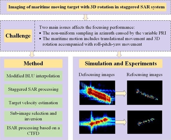
Imaging maritime targets requires a high resolution and wide swath (HWRS) in a synthetic aperture radar (SAR). When operated with a variable pulse repetition interval (PRI), a staggered SAR can realize HRWS imaging, which needs to be reconstructed due to echo pulse loss and a nonuniformly sampled signal along the azimuth. The existing reconstruction algorithms are designed for stationary scenes in a staggered SAR mode, and thus, produce evident image defocusing caused by complex target motion for moving targets. Typically, the nonuniform sampling and complex motion of maritime targets aggravate the spectrum aliasing in a staggered SAR mode, causing inevitable ambiguity and degradation in its reconstruction performance. To this end, this study analyzed the spectrum of maritime targets in a staggered SAR system through theoretical derivation. After this, a reconstruction method named MBLCFD (Modified Best Linear Unbaised and Complex-Lag Time-Frequency Distribution) is proposed to refocus the blurred maritime target. First, the signal model of the maritime target with 3D rotation accompanying roll–pitch–yaw movement was established under the curved orbit of the satellite. The best linear unbiased (BLU) method was modified to alleviate the coupling of nonuniform sampling and target motion. A precise SAR algorithm was performed based on the method of inverse reversion to counteract the effect of a curved orbit and wide swath. Based on the hybrid SAR/ISAR technique, the complex-lag time-frequency distribution was exploited to refocus the maritime target images. Simulations and experiments were carried out to verify the effectiveness of the proposed method, providing precise refocusing performance in staggered mode.

1. Introduction

With the development of various synthetic aperture radar (SAR) systems [1,2], the next generation of spaceborne SAR requires a high resolution and wide swath, especially for maritime surveillance applications. High-spatial-resolution SAR images facilitate the detection and imaging of small-to-medium-sized maritime targets, providing reliable information for subsequent localization, identification, and interpretation [3,4]. A wide swath, which is characterized by a short revisit time, proves to be beneficial for discovering and monitoring dynamic targets in a wide maritime area. Compared with traditional SAR systems, the HRWS SAR configuration imposes higher requirements on maritime moving target imaging. In addition to the inherent spatial displacement and defocusing issues caused by target motion, it is essential to address the impact of the HRWS SAR configuration itself, such as multiple beams or a variable pulse repetition interval (PRI), on moving target imaging.

The existing high-resolution and wide swath (HRWS) systems are mainly proposed for imaging stationary scenes, while the application for monitoring moving targets is limited since the complex target motion produces evident image defocusing. A typical HRWS SAR system adopts multiple RX channels arranged along the azimuth. Due to the similar system architecture, this system combines moving target indication (MTI) systems to realize clutter suppression and moving target imaging [5]. However, operating with a low pulse repetition frequency (PRF) exaggerates the azimuth ambiguities of the moving targets, along with the long antenna and the expense of high system complexity.

Without the necessity to lengthen the antenna, a staggered SAR has greatly advanced the HRWS system by combining multiple elevation beam (MEB) technology and a variable PRI, which has been adopted in Tandem-L [6,7] and NISAR satellites [8]. The technology of multiple elevation beams (MEBs) provides an attractive solution for mapping an ultra-wide swath with a high resolution. The entire wide swath is illuminated by a wide beam on transmit, and the multiple elevation beams sweep following the directions of echo arrival to simultaneously map multiple subswaths. In a conventional MEB SAR system [9] with a constant PRI, there will be constant blind areas due to the coincidence of transmitting and receiving events, resulting in gaps in the whole swath.

When operated with a variable PRI, a staggered SAR can address the problems of the constant blind areas to achieve gapless observation [10,11]. Meanwhile, the cost is that the variable PRI leads to lost pulses and nonuniformly sampled signals along the azimuth. To enable subsequent SAR processing, it is essential to reconstruct the nonuniform echo signal into the uniformly sampled signal. A number of reconstruction algorithms have been proposed, including the best linear unbiased (BLU) interpolation [12], missing data iterative adaptive algorithm (MIAA) [13], and other methods [14,15,16].

These existing reconstruction methods achieve good performance for a stationary scene. However, reconstructing the echoes of moving targets will produce evident image defocusing caused by complex target motion. Recently, scholars have turned their attention to the investigation of a staggered SAR for motion target detection, primarily emphasizing system design and detection methodologies, which have achieved impressive results [17,18]. However, little can be found in the literature about imaging the moving targets in a staggered SAR system. Actually, the complex target motion and the nonuniform azimuth sampling are two main issues that affect the focusing performance of moving targets in a staggered SAR. The maritime target motion includes translational movement and three-dimensional rotation accompanied with roll–pitch–yaw movement. Both of these can lead to blurred and displaced images. The nonuniform sampling causes spectrum aliasing along the azimuth, which is aggravated by the Doppler center due to target translational motion. These two issues interact, causing inevitable ambiguity and degrading the reconstruction performance. To solve this problem, this paper proposes a reconstruction algorithm for moving target imaging in a staggered SAR system.

Overall, motivated by the BLU and hybrid SAR/ISAR techniques, our contributions in this paper are summarized as follows:

(1) The spectrum of maritime moving targets was derived in staggered mode. The derivation indicates that the complex target motion coupled with nonuniform sampling greatly aggravates image defocusing.

(2) Inspired by hybrid SAR/ISAR technology [19], a novel reconstruction algorithm named MBLCFD is proposed to image the maritime targets with three-dimensional rotation in staggered mode. The BLU algorithm was modified after roughly estimating the target translational velocity. An accurate SAR processing method was used based on the method of inverse reversion to counteract the range and Doppler migration caused by the curved orbit, the wide swath, and the target motion. The complex-lag time-frequency distribution (CTFD) was carried out to refocus the maritime moving target images.

(3) In addition, compared with its rivals, the proposed algorithm provided superior refocusing performance in terms of the main lobe width (MW), peak-to-sidelobe ratio (PSLR), and integration sidelobe ratio (ISLR) for maritime moving targets in a staggered SAR system.

The remainder of this paper is organized as follows: Section 2 establishes the geometric configuration and signal model in a staggered SAR mode. The spectrum of echo signal for maritime moving targets is derived in Section 3. Derivations show that the complex motion of the maritime target, coupled with nonuniform sampling, aggravates the spectrum aliasing and the azimuth ambiguity. To address this issue, the proposed MBLCFD reconstruction is presented in Section 4. In Section 5, simulated data and equivalent raw data are employed to verify the feasibility and effectiveness of the proposed algorithm. A brief conclusion is given in Section 6.

2. Geometric Configuration and Signal Model

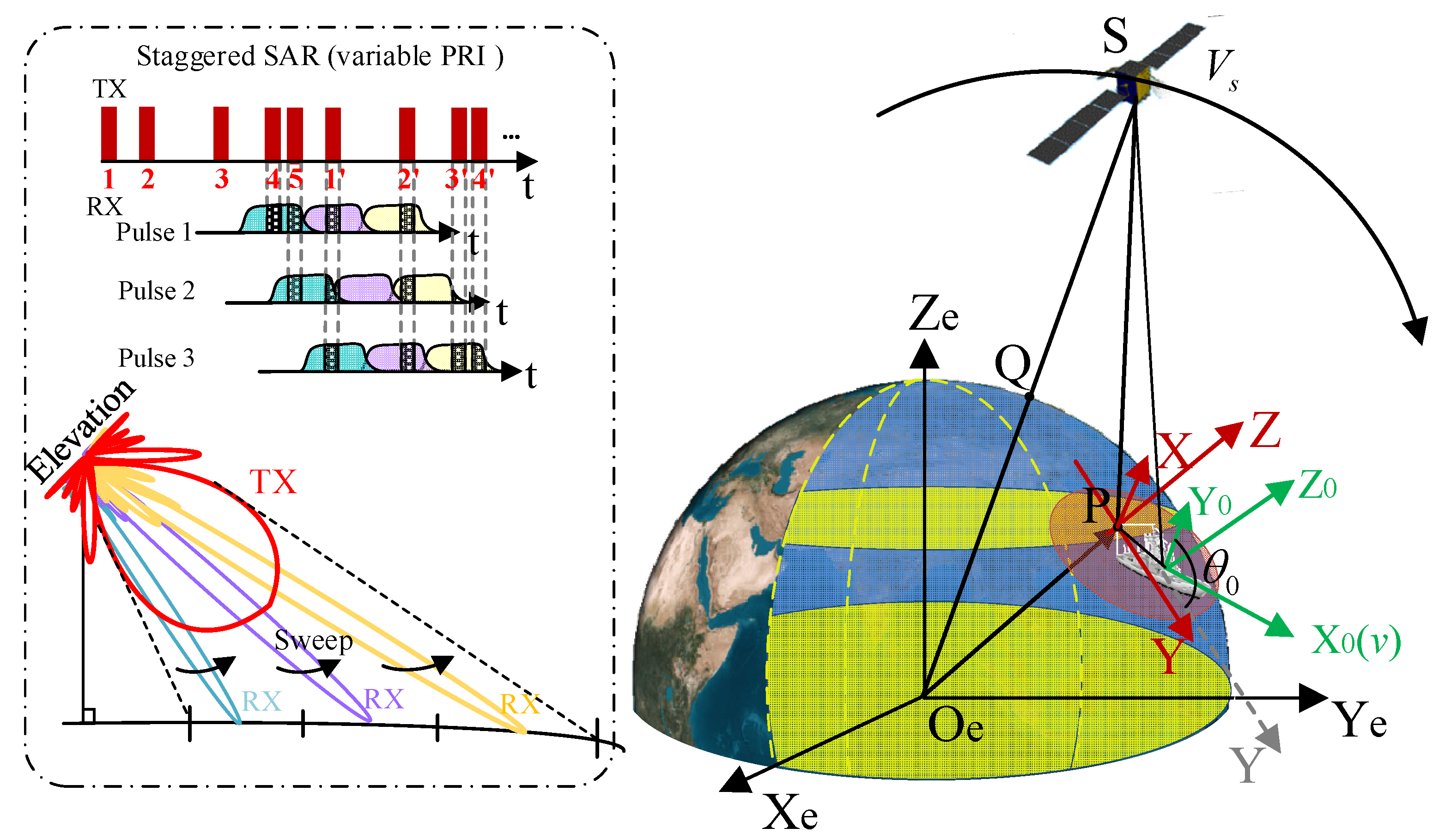
The geometry of the staggered SAR for maritime targets is depicted in Figure 1. In the Earth rectangular coordinates (ERCs) $O_e\text{-}{X}_e{Y}_e{Z}_e$, $O_e$ denotes the Earth’s center. The $O_e{X}_e$-axis follows the Greenwich meridian direction, and the $O_e{Z}_e$-axis follows the Earth’s angular momentum direction. The beam-pointing direction and the Earth’s surface intersect at P. Assume that P is the origin of the imaging scene coordinate $P\text{-}XYZ$. The $PZ$-axis is oriented toward the Earth’s center. The $PY$-axis is located within $SQP$ and is perpendicular to the $PZ$-axis. $\phi$ denotes the radar look angle. Considering the Earth’s angular velocity and the curved orbit, the radar’s position ${\mathit{R}}_{\mathit{s}}\left(t_a\right)$ in the $P\text{-}XYZ$ coordinate is obtained in [20].

The target coordinate $P\text{-}{X}_0{Y}_0{Z}_0$ is established by rotating $P\text{-}XYZ$ clockwise along the Z-axis with ${\theta }_0$. $P{X}_0$ is along the direction of the ship’s bow. ${\mathit{R}}_{\mathit{T}}$ denotes the vector from the point P to the target. Thus, the position of the satellite in the target coordinates is ${\mathit{R}}_{\mathit{s}\mathit{0}}\left(t_a\right)={\mathit{R}}_{{\theta }_{\mathit{0}}}·{\mathit{R}}_{\mathit{s}}\left(t_a\right)+{\mathit{R}}_{\mathit{T}}$. ${\mathit{R}}_{{\theta }_{\mathit{0}}}$ is the rotation matrix. The ship target has a translational motion along $X_0$ with a velocity of v, which is denoted as ${\mathit{V}}_T={\left[v_{Tx},v_{Ty},0\right]}^T$ in $P\text{-}XYZ$. The position of a scatter point i on the ship target is ${[x_{i0},y_{i0},z_{i0}]}^{\mathrm{T}}$ at the initial moment.

After the hull has been constructed in three dimensions, the location of the point i in the target coordinate ${\mathit{R}}_{\mathit{i}\mathit{0}}\left(t_a\right)$ is given by

$${\mathit{R}}_{\mathit{i}\mathit{0}}\left(t_a\right)=\mathfrak{R}\left(t_a\right){\left[x_{i0},y_{i0},z_{i0}\right]}^T+{\left[v{t}_a,0,0\right]}^T$$

(1)

where $\mathfrak{R}\left(t_a\right)={\mathit{R}}_{\mathrm{roll}}\left(t_a\right){\mathit{R}}_{\mathrm{pittl}}\left(t_a\right){\mathit{R}}_{\mathrm{yaw}}\left(t_a\right)$ is the rotation matrix is the superposition of the effects of pitch, yaw, and roll directions. The rotation matrices ${\mathit{R}}_{\mathrm{roll}}\left(t_a\right)$, ${\mathit{R}}_{\mathrm{pitch}}\left(t_a\right)$, and ${\mathit{R}}_{\mathrm{yaw}}\left(t_a\right)$ can be expressed as

$${\mathit{R}}_{\mathrm{roll}}\left(t_a\right)=\left[\begin{array}{ccc}1& 0& 0\\ 0& cos{\theta }_{\mathrm{roll}}\left(t_a\right)& -sin{\theta }_{\mathrm{roll}}\left(t_a\right)\\ 0& sin{\theta }_{\mathrm{roll}}\left(t_a\right)& cos{\theta }_{\mathrm{roll}}\left(t_a\right)\end{array}\right]$$

(2)

$${\mathit{R}}_{\mathrm{pitch}}\left(t_a\right)=\left[\begin{array}{ccc}cos{\theta }_{\mathrm{pitch}}\left(t_a\right)& 0& -sin{\theta }_{\mathrm{pitch}}\left(t_a\right)\\ 0& 1& 0\\ sin{\theta }_{\mathrm{pitch}}\left(t_a\right)& 0& cos{\theta }_{\mathrm{pitch}}\left(t_a\right)\end{array}\right]$$

(3)

$${\mathit{R}}_{\mathrm{yaw}}\left(t_a\right)=\left[\begin{array}{ccc}cos{\theta }_{\mathrm{yaw}}\left(t_a\right)& -sin{\theta }_{\mathrm{yaw}}\left(t_a\right)& 0\\ sin{\theta }_{\mathrm{yaw}}\left(t_a\right)& cos{\theta }_{\mathrm{yaw}}\left(t_a\right)& 0\\ 0& 0& 1\end{array}\right]$$

(4)

The rotation follows sinusoidal motion [21]:

$${\theta }_{\xi }\left(t_a\right)=\frac{1}{2}{A}_{\xi }sin\left(2\pi \frac{t_a}{{\tau }_{\xi }}+{\varphi }_{\xi }\right),\xi =\mathrm{roll},\mathrm{pitch},\mathrm{yaw}$$

(5)

where $A_{\xi }$ denotes the amplitude of the rotation, $T_{\xi }$ represents the rotation period, and ${\psi }_{\xi }$ is the initial phase of the rotation. These parameters are related to the sea state, the maritime target types, the velocities, and so on.

The slant range between the satellite and the scatterer i can be expressed as

$$\begin{array}{cc}\hfill & R_{si}\left(t_a\right)=\left|{\mathit{R}}_{\mathit{si}}\left(t_a\right)\right|=\left|{\mathit{R}}_{\mathit{s}\mathit{0}}\left(t_a\right)-{\mathit{R}}_{\mathit{i}\mathit{0}}\left(t_a\right)\right|\approx \left(k_0+\Delta k_0\right)+\hfill \\ \hfill & \left(k_1+\Delta k_1\right)t_a+\left(k_2+\Delta k_2\right)t_a^2+\left(k_3+\Delta k_3\right)t_a^3\hfill \end{array}$$

(6)

where $k_0$, $k_1$, $k_2$, and $k_3$ are the terms of Taylor series caused by the satellite motion [22], and $\Delta k_0$, $\Delta k_1$, $\Delta k_2$, and $\Delta k_3$ denote the terms induced in the target motion. The $k_0$, $k_1$, $k_2$, and $k_3$ can be obtained by

$$k_0=\frac{{\mathit{R}}_{\mathit{si}}·{\mathit{R}}_{\mathit{si}}}{k_0}$$

(7)

$$k_1={\left.\frac{\partial R_{si}\left(t_a\right)}{t_a}\right|}_{t_a=0}=\frac{{\mathit{R}}_{\mathit{si}}·{\mathit{V}}_{\mathit{s}\mathit{0}}}{k_0}$$

(8)

$$k_2=\frac{1}{2}\times {\left.\left(\frac{{\partial }^2{R}_{si}\left(t_a\right)}{\partial t_a^2}\right)\right|}_{t_a=0}=\frac{{\mathit{V}}_{\mathit{s}\mathit{0}}·{\mathit{V}}_{\mathit{s}\mathit{0}}+{\mathit{A}}_{\mathit{s}\mathit{0}}·{\mathit{R}}_{\mathit{si}}}{2k_0}$$

(9)

$$k_3=\frac{1}{3!}\times {\left.\left(\frac{{\partial }^3{R}_{si}\left(t_a\right)}{t_a^3}\right)\right|}_{t_a=0}=\frac{{\mathit{B}}_{\mathit{s}\mathit{0}}·{\mathit{R}}_{\mathit{si}}+3{\mathit{A}}_{\mathit{s}\mathit{0}}{\mathit{V}}_{\mathit{s}\mathit{0}}}{6k_0}+\frac{k_1^3-k_1\left({{\mathit{V}}_{\mathit{s}\mathit{0}}}^2+{\mathit{A}}_{\mathit{s}\mathit{0}}·{\mathit{R}}_{\mathit{si}}\right)}{2k_0^2}$$

(10)

where ${\mathit{V}}_{\mathit{s}\mathit{0}}$, ${\mathit{A}}_{\mathit{s}\mathit{0}}$, and ${\mathit{B}}_{\mathit{s}\mathit{0}}$ represent the velocity vector, acceleration vector, and second-order acceleration vector of the satellite.

In a staggered SAR, the entire wide swath is illuminated by a wide beam on transmit as shown in Figure 1, and the multiple elevation beams sweep following the directions of echo arrival to simultaneously map multiple subswaths. When operated with the variable PRIs, the blind areas appear at varying slant ranges for different echo pulses, allowing for mapping a wide continuous swath. The pulses are transmitted with different PRIs denoted as $PR{I}_m,m=0,1,\dots ,M$. After this, the M pulses repeat periodically. Thus, the ath pulse is transmitted at the slow time $t_a$:

$$t_a=⌊\frac{a}{M}⌋T_{sw}+\sum _{m=0}^{a-\lfloor a/M\rfloor ·M-1}PR{I}_m$$

(11)

where the period $T_{sw}={\sum }_{m=0}^{M-1}PR{I}_m$. The echo signal after demodulation is represented as follows:

$$\begin{array}{cc}\hfill & S_r\left(t_r,t_a\right)=\sum _{i}B(t_r,t_a){\sigma }_i{w}_{\mathrm{r}}\left(\frac{t_r-2R_{si}\left(t_a\right)/c}{T_{\mathrm{p}}}\right)w_{\mathrm{a}}\left(t_a\right)\hfill \\ \hfill & \times exp\left[j\left(-\frac{4\pi }{\lambda }{R}_{si}\left(t_a\right)+\pi \gamma {\left(t_r-\frac{2R_{si}\left(t_a\right)}{c}\right)}^2\right)\right]\hfill \end{array}$$

(12)

where $t_r$ is the fast time. ${\sigma }_i$ is the scattering coefficient of the ith scatter point. The wavelength and chirp rate are expressed as $\lambda$ and $\gamma$, respectively. $w_a(·)$ refers to the azimuth envelope. The blind range matrix $B(t_r,t_a)$ equals 0 when the pulse is lost and equals 1 when the pulse is fully received.

3. The Spectrum of Maritime Target Echoes for Staggered SAR

The spectrum of maritime targets at the azimuth is derived based on the uniformly sampled spectrum. The received M nonuniform samples within one period can be considered as M channels. Assuming that the first channel is the reference channel $S_{ref}\left(t_a\right)$, the signal of the mth channel is given as

$$S_m\left(t_a\right)=\sum _{k=-\infty }^{+\infty }{S}_{ref}(t_a-\Delta t_m)\delta (t_a-k{T}_{sw})+n_m\left(t_a\right)$$

(13)

where $\Delta t_m$ is the time delay of the mth channel relative to the reference channel. $n_m\left(t_a\right)$ denotes the noise. $S_{ref}\left(t_a\right)$ is the reference echo signal of the maritime target sampled uniformly at the azimuth. Equation (13) can be rewritten as

$$\begin{array}{cc}\hfill S_a\left(t_a\right)& =\sum _{k=-\infty }^{+\infty }\delta \left(t_a-k{T}_{sw}\right)\left[S_{ref}\left(t_s\right)+S_{ref}\left(t_a-\Delta t_1\right)+\cdots +S_{ref}\left(t_a-\Delta t_{M-1}\right)\right]+n_m\left(t_a\right)\hfill \\ \hfill & =\sum _{m=0}^{M-1}\sum _{k=-\infty }^{+\infty }{S}_{ref}\left(t_a-\Delta t_m\right)\delta \left(t_a-k{T}_{sw}\right)+n_m\left(t_a\right)\hfill \end{array}$$

(14)

Equation (14) can be written in the discrete time domain as

$$\begin{array}{cc}\hfill S_a\left(k\right)& ={\left.S_a\left(t_a\right)\right|}_{t_a=k{T}_{sw}}+{\left.S_a\left(t_a\right)\right|}_{t_a=k{T}_{sw}-\Delta t_1}+\cdots +{\left.S_a\left(t_a\right)\right|}_{t_a=k{T}_{sw}-\Delta t_{M-1}}\hfill \\ \hfill & ={\left.\sum _{m=0}^{M-1}{S}_a\left(t_a\right)\right|}_{t_a=k{T}_{sw}-\Delta t_m}\hfill \end{array}$$

(15)

The nonuniformly sampled signal in the discrete-time domain for the staggered mode can also be represented by

$$\begin{array}{cc}\hfill S_a\left(k\right)& ={\left.\sum _{m=0}^{M-1}{S}_a\left(t\right)\right|}_{t=k{T}_{sw}-\Delta t_m}=\sum _{m=0}^{M-1}\frac{1}{2\pi }{\int }_{-\infty }^{+\infty }{S}_a(j\Omega )exp\left(j\Omega \left(k{T}_{sw}-\Delta t_m\right)\right)d\Omega \hfill \\ \hfill & =\sum _{m=0}^{M-1}\frac{1}{2\pi }\sum _{r=-\infty }^{+\infty }{\int }_{\frac{2\pi }{T_{sw}}r-\frac{\pi }{T_{sw}}}^{\frac{2\pi }{T_{sw}}r+\frac{\pi }{T_{sw}}}{S}_a(j\Omega )exp\left[j\Omega \left(k{T}_{sw}-\Delta t_m\right)\right]d\Omega \hfill \end{array}$$

(16)

Assuming that ${\Omega }^{\prime }=\Omega -\frac{2\pi }{T_{sw}}r$, Equation (16) can be rewritten as

$$\begin{array}{cc}\hfill S_a\left(k\right)& =\sum _{m=0}^{M-1}\frac{1}{2\pi }\sum _{r=-\infty }^{+\infty }{\int }_{-\frac{\pi }{T_{sw}}}^{\frac{\pi }{T_{sw}}}{S}_a\left(j{\Omega }^{\prime }+j\frac{2\pi }{T_{sw}}r\right)exp\left(j{\Omega }^{\prime }k{T}_{sw}\right)exp\left[-j\left({\Omega }^{\prime }+\frac{2\pi }{T_{sw}}r\right)\Delta t_m\right]d{\Omega }^{\prime }\hfill \\ \hfill & =\sum _{m=0}^{M-1}\frac{1}{2\pi T_{sw}}\sum _{r=-\infty }^{+\infty }{\int }_{-\pi }^{\pi }{S}_a\left(j\frac{w}{T_{sw}}+j\frac{2\pi }{T_{sw}}r\right)exp\left(jkw\right)exp\left[-j\left(\frac{w}{T_{sw}}+\frac{2\pi }{T_{sw}}r\right)\Delta t_m\right]dw\hfill \end{array}$$

(17)

According to the discrete-time Fourier transform (DTFT), $S_a\left(k\right)$ can also be provided by

$$S_a\left(k\right)=\frac{1}{2\pi }{\int }_{-\pi }^{\pi }{S}_a\left(jw\right)exp\left(jwk\right)dw$$

(18)

Comparing Equations (17) and (18), the following can be obtained:

$$\begin{array}{cc}\hfill & S_a\left(jw\right)=\sum _{m=0}^{M-1}\frac{1}{2\pi T_{sw}}\sum _{r=-\infty }^{+\infty }{\int }_{-\pi }^{\pi }{S}_{ref}\left(j\frac{w}{T_{sw}}+j\frac{2\pi }{T_{sw}}r\right)exp\left(jkw\right)\hfill \\ \hfill & ·exp\left[-j\left(\frac{w}{T_{sw}}+\frac{2\pi }{T_{sw}}r\right)\Delta t_m\right]dw\hfill \end{array}$$

(19)

Thus, it is not difficult to derive the azimuth spectrum of the echo signal of maritime targets as

$$\begin{array}{cc}\hfill & S_a\left(f_a\right)=\sum _{r=-\infty }^{\infty }{S}_{ref}\left(M(f_a+r·F_{sw})\right)\hfill \\ \hfill & ·\left[\sum _{m=0}^{M-1}exp\left(-j2\pi (f_a+r·F_{sw})\Delta t_m\right)\right]+N\left(f_a\right)\hfill \\ \hfill & =\sum _{r=-\infty }^{\infty }{S}_{ref}(f_a+r·F_{sw})+S_{ref}^{amb}(f_a+r·F_{sw})+N\left(f_a\right)\hfill \end{array}$$

(20)

where $F_{sw}=1/T_{sw}$ and $\Delta t_0=0$. $S_{ref}^{amb}(·)$ denotes the sum of terms when $m=1,\dots ,M-1$. $N\left(f_a\right)$ denotes the noise spectrum. $PR{F}_{\mathrm{mean}}$ denotes the geometric mean PRF on transmit of the staggered SAR system, i.e., $PR{F}_{\mathrm{mean}}=\sqrt{PR{F}_{\max }·PR{F}_{\min }}$, where $PR{F}_{\max }$ and $PR{F}_{\min }$ denote the maximum and minimum of the PRI sequence, respectively.

As shown in Figure 2, for the static target, the spectrum aliasing mainly arises from two aspects. One is the multiple pairs of uniformly distributed weak aliasing $S_{ref}^{amb}(f_a+r{F}_{sw})$ caused by nonuniform sampling, as denoted by the blue dotted lines. The other is the spectrum aliasing caused by a non-ideal antenna pattern (sinc-like pattern), as shown in the green dashed line. For the moving target, the Doppler center is shifted to $f_{dc}$. The target motion and the nonuniform sampling are coupled. Consequently, within $\left[-PR{F}_{\mathrm{mean}}/2,PR{F}_{\mathrm{mean}}/2\right]$, the spectrum aliasing $S_{ref}^{amb}(f_a+r{F}_{sw})$ caused by the nonuniform sampling is aggravated, which further causes inevitable ambiguities and degrades the imaging performance.

4. Image Reconstruction of Maritime Targets for Staggered SAR System

Figure 3 depicts the flowchart of the proposed MBLCFD algorithm, which is summarized as follows.

Step 1 (modified BLU interpolation): The BLU interpolation is operated with the power spectral density (PSD). The PSD is proportional to the antenna power pattern [12]. Considering the translational target velocity, the modified PSD of the raw azimuth signal $u\left(t_a\right)$ for the moving target can be expressed as

$$P_u\left(f_a\right)={sin}^4\left(\pi \frac{L_a}{2(v_s-v_{Tx})}{f}_a\right)/{\left(\pi \frac{L_a}{2(v_s-v_{Tx})}{f}_a\right)}^4$$

(21)

where $v_s$ and $v_{Tx}$ denote the translational velocities of the satellite and the target along the track. $L_a$ denotes the synthetic aperture length. The autocorrelation function $R_u\left(\xi \right)$ of the complex-valued stochastic process $u\left(t_a\right)$ is obtained through the inverse Fourier transform of its PSD:

$$\begin{array}{cc}\hfill R_u\left(\xi \right)=& \frac{E\left\{u^{*}\left(t_a\right)u(t_a+\xi )\right\}}{E\left\{|u\left(t_a\right){|}^2\right\}}\hfill \\ \hfill =& {\left(\frac{v_s-v_{Tx}}{L_a}\right)}^3\left[6{\xi }^{3}sign\left(\xi \right)+{\left(\xi -\frac{L_a}{v_s-v_{Tx}}\right)}^{3}sign\left(\xi -\frac{L_a}{v_s-v_{Tx}}\right)\right.\hfill \\ \hfill & +4{\left(-\xi +\frac{L_a}{2v_s-v_{Tx}}\right)}^{3}sign\left(\xi -\frac{L_a}{2v_s-v_{Tx}}\right)+4{\left(\xi +\frac{L_a}{2v_s-v_{Tx}}\right)}^3\hfill \\ \hfill & \left.·sign\left(\xi +\frac{L_a}{2v_s-v_{Tx}}\right)+{\left(\xi +\frac{L_a}{v_s-v_{Tx}}\right)}^{3}sign\left(\xi +\frac{L_a}{v_s-v_{Tx}}\right)\right]\hfill \end{array}$$

(22)

The PSD can also be considered as the convolution of two square functions of the sinc function. Given that the square of the sinc function corresponds to the Fourier transform of the triangular function, $R_u\left(\xi \right)$ can thus be regarded as the convolution of two triangular functions. Additionally, considering the illumination time at the azimuth, $R_u\left(\xi \right)$ should satisfy

$$R_u\left(\xi \right)=0,\left|\xi \right|\ge \frac{L_a}{v_s-v_{Tx}}$$

(23)

In the presence of the additive white Gaussian random noise, the correlation function can be expressed as

$$R_{un}\left(\xi \right)=\frac{1}{SNR}\delta \left(\xi \right)+\frac{SNR-1}{SNR}{R}_u\left(\xi \right)$$

(24)

where SNR represents the signal-to-noise ratio, and $\delta (·)$ is the Kronecker delta function.

The nonuniform sampling $u\left(t_a\right)$ is used to estimate the uniform sampling $u\left(t_u\right)$. The uniformly sampled azimuth signal is reconstructed by the optimal linear unbiased estimation interpolation [12] using

$$\widehat{u}\left(t_u\right)={\mathbf{u}}^{\mathrm{T}}{\mathbf{G}}^{-1}\mathbf{r}$$

(25)

where $\mathbf{u}={\left[u\left(t_1\right),\cdots ,u\left(t_q\right),\cdots u\left(t_{N_a}\right)\right]}^T$ is the nonuniform sampling at the azimuth. $\mathbf{r}$ is a column vector. The qth element in $\mathbf{r}$ equals $r_q=R_{un}\left(t^{\prime }-t_q\right)$, where $q=1,\dots ,N_a$. The $qs$th element in G equals $g_{qs}=R_{un}\left(t_q-t_s\right)$ for $q=1,\dots ,N_a$ and $s=1\dots N_a$. $R_{un}$ is the correlation function of the signal and noise.

Remark 1: Using the information about the target velocity, the modified BLU can alleviate the coupling of the nonuniform sampling and the target motion. The target velocity is roughly obtained by the estimation of the Doppler center and Doppler rate. The former is estimated by the correlation function, and the latter is estimated by the minimum entropy method. The accuracy of the estimation of the target translational velocity is limited, as the 3D rotation exists and the satellite ephemeris data used would be slightly different from the actual satellite motion.

Remark 2: Compared with the traditional BLU interpolation, the modified BLU interpolation can effectively reconstruct the nonuniform azimuth sampling into a uniform grid. However, the modified BLU interpolation still achieves the rough reconstruction, and the reconstruction performance is limited. As is apparent from (21) and (22), the translational target velocity along the track is considered in the PSD and the autocorrelation function. Actually, the radial velocity and the 3D rotation of the target also have an influence on the reconstruction performance. The Doppler shift caused by the radial velocity does not change the shape of the PSD and the amplitude of the autocorrelation function, which indicates a slight influence on the reconstruction performance. The influence of the radial velocity is alleviated in the subsequent step 3. After this, due to the limited accuracy of target velocity estimation, there is still residual translational motion that requires further fine compensation in subsequent processing. The residual translational motion and the 3D rotation are accurately compensated in step 5.

Step 2 (staggered SAR processing): Using the estimation of the target velocity, SAR image processing is performed to compensate for the movement of the radar platform and the translational motion of the target. Exploiting the method of series reversion, the 2D Fourier transform (FT) is used to obtain a 2D spectrum of echo signal after range compression. The details are described as follows:

Performing the Fourier transform in Equation (12), it can be obtained that

$$S_r\left(f_r,t_a\right)={\int }_{-\infty }^{\infty }{S}_r\left(t_r,t_a\right)exp\left\{-j2\pi f_r{t}_r\right\}d{t}_r$$

(26)

Combining Equations (12) and (26), the phase within the integral can be expressed as

$$\theta \left(t_r\right)=-\frac{2\pi f_c{R}_{si}\left(t_a\right)}{c}+\pi \gamma {\left(t_r-\frac{R_{si}\left(t_a\right)}{c}\right)}^2-2\pi f_r{t}_r$$

(27)

where c is the speed of light. Taking the derivative of Equation (27), we can obtain

$$\frac{d\theta \left(t_r\right)}{d{t}_r}=2\pi \gamma \left(t_r-\frac{R_{si}\left(t_a\right)}{c}\right)-2\pi f_r{t}_r$$

(28)

Assuming that $d\theta \left(t_r\right)/d{t}_r=0$, the relationship between the fast time frequency $f_r$ and the fast time $t_r$ is

$$t_r=\frac{f_r}{\gamma }+\frac{R_{si}\left(t_a\right)}{c}$$

(29)

According to the principle of the stationary phase, Equation (26) can be expressed as

$$\begin{array}{c}\hfill S_r\left(f_r,t_a\right)=\sum _{i}B\left(f_r,t_a\right)W_r\left(f_r\right)w_a\left(t_a\right)exp\left\{-j\frac{\pi f_r^2}{\gamma }\right\}exp\left\{-\frac{j2\pi \left(f_c+f_r\right)}{c}\times \right.\\ \hfill \left.\left[\left(2k_0+\Delta k_0\right)+\left(2k_1+\Delta k_1\right)·t_a+\left(2k_2+\Delta k_2\right)·t_a^2+\left(2k_3+\Delta k_3\right)·t_a^3\right]\right\}\end{array}$$

(30)

Similarly, performing an azimuthal Fourier transform on (30), the following can be derived:

$$S_{2dr}\left(f_r,f_a\right)={\int }_{-\infty }^{\infty }{S}_r\left(f_r,t_a\right)exp\left\{-j2\pi f_a{t}_a\right\}d{t}_a$$

(31)

Combining Equations (30) and (31), the phase within the integral can be expressed as

$$\begin{array}{cc}\hfill \theta \left(t_a\right)=& -\frac{\pi f_r^2}{\gamma }-2\pi f_a{t}_a-\frac{2\pi \left(f_c+f_r\right)}{c}\times \left[\left(2k_0+\Delta k_0\right)\right.\hfill \\ \hfill & +\left(2k_1+\Delta k_1\right)·t_a+\left(2k_2+\Delta k_2\right)·t_a^2+\left(2k_3+\Delta k_3\right)·t_a^3\hfill \end{array}$$

(32)

Assuming that $d\theta \left(t_r\right)/d{t}_r=0$, it can be obtained that

$$-\frac{c}{f_c+f_r}{f}_a=\left(2k_1+\Delta k_1\right)+2\left(2k_2+\Delta k_2\right)·t_a+3\left(2k_3+\Delta k_3\right)·t_a^2$$

(33)

Applying the method of series reversion, the slow time can be rewritten as

$$t_a\left(f_a\right)=L_1·\left(-\frac{c}{f_c+f_r}{f}_a-L_0\right)+L_2·{\left(-\frac{c}{f_c+f_r}{f}_a-L_0\right)}^2$$

(34)

where

$$L_0=2k_1+\Delta k_1$$

(35)

$$L_1=1/2\left(2k_2+\Delta k_2\right)$$

(36)

$$L_2=3\left(2k_3+\Delta k_3\right)/8{\left(2k_2+\Delta k_2\right)}^3$$

(37)

Using Equation (34) and the principle of stationary phase, the 2D spectrum of the echo signal after range compression can be obtained as

$$S_{2dr}\left(f_r,f_a\right)=\sum _{t}B\left(f_r,f_a\right)W_r\left(f_r\right)W_a\left(f_a-f_{ac}\right)exp\left\{j{\theta }_a\left(f_r,f_a\right)\right\}$$

(38)

where $B(f_r,f_a)$ is the blind area matrix. $W_r\left(f_r\right)$ is the range envelope in the frequency domain. $W_a\left(f_a-f_{ac}\right)$ represents the azimuthal spectral envelope with $f_{ac}$ as the Doppler center frequency. ${\theta }_a\left(f_r,f_a\right)$ is the phase term, which can be expressed as

$$\begin{array}{cc}\hfill {\theta }_a\left(f_r,f_a\right)& =-\frac{\pi f_r^2}{\gamma }-\frac{2\pi \left(f_c+f_r\right)}{c}\left(2k_0+\Delta k_0\right)+2\pi L_0{L}_1\left(f_a+\frac{L_0·\left(f_c+f_r\right)}{c}\right)\hfill \\ \hfill & -\frac{\pi L_{1}c}{f_c+f_r}{\left(f_a+\frac{L_0·\left(f_c+f_r\right)}{c}\right)}^2+\frac{2\pi L_2{c}^2}{3{\left(f_c+f_r\right)}^2}{\left(f_a+\frac{L_0·\left(f_c+f_r\right)}{c}\right)}^3\hfill \end{array}$$

(39)

Utilizing a Taylor series expansion of ${\left(f_c+f_r\right)}^{-n}$, the above expression can be further rewritten as

$$\begin{array}{cc}\hfill & S_{2\mathrm{df}}\left(f_r,f_a\right)=W(f_r,f_a)exp\left\{j2\pi {\varphi }_{az}\left(f_a\right)\right\}-exp\left\{-j2\pi {\varphi }_{RP}\right\}\hfill \\ \hfill & exp\left\{-j2\pi B_1\left(f_a\right)f_r\right\}exp\left\{-j\pi B_2\left(f_a\right)f_r^2\right\}exp\left\{-j2\pi B_3\left(f_a\right)f_r^3\right\}\hfill \end{array}$$

(40)

The ${\varphi }_{az}\left(f_a\right)$, ${\varphi }_{RP}$, $B_1\left(f_a\right)$, $B_2\left(f_a\right)$, and $B_3\left(f_a\right)$ are given as

$${\varphi }_{az}\left(f_a\right)=L_0^2{L}_2·f_a-\left(\frac{L_{1}c}{2f_c}-\frac{L_0{L}_{2}c}{f_c}\right)·f_a^2+\frac{L_2{c}^2}{3f_c^2}·f_a^3$$

(41)

$${\varphi }_{RP}=-\frac{L_0^2{L}_1{f}_c}{2c}-\frac{L_0^3{L}_2{f}_c}{3c}+\frac{f_c}{c}\left(2k_0+\Delta k_0\right)$$

(42)

$$\begin{array}{cc}\hfill B_1\left(f_a\right)=& -\frac{L_0^2{L}_1}{2c}-\frac{L_0^3{L}_2}{3c}+\frac{L_{1}c·f_a^2}{2f_c^2}+\frac{L_0{L}_{2}c·f_a^2}{f_c^2}\hfill \\ \hfill & +\frac{2L_2{c}^2·f_a^3}{3f_c^3}+\frac{2k_0+\Delta k_0}{c}\hfill \end{array}$$

(43)

$$B_2\left(f_a\right)=-\frac{L_{1}c·f_a^2}{f_c^3}-\frac{2L_0{L}_{2}c·f_a^2}{f_c^3}-\frac{2L_2{c}^2·f_a^3}{f_c^4}+\frac{1}{K_r}$$

(44)

$$B_3\left(f_a\right)=\frac{L_{1}c·f_a^2}{2f_c^4}+\frac{3L_0{L}_{2}c·f_a^2}{f_c^4}+\frac{4L_2{c}^2·f_a^3}{3f_c^5}$$

(45)

The compensation functions defined in (43)–(45) provide a range migration compensation, residual range compensation, and higher order phase compensation, respectively. These compensation functions are used to multiply the received signals, and then the inverse Fourier transform in range is performed. The azimuth compression is carried out by convolving the signals with (41).

Step 3 (target velocity estimation): Estimating the Doppler center and Doppler rate after the range compression. The Doppler center is estimated by the correlation function method, where $f_{dc}^{\prime }$ is obtained by the peak of the power spectrum. The Doppler rate $f_{dr}^{\prime }$ is estimated by an iterative search to minimize the image entropy.

Subsequently, the translational velocity of the target ${\mathit{V}}_{\mathit{T}}={\left[v_{Tx},v_{Ty},v_{Tz}\right]}^T$ is estimated from $f_{dc}^{\prime }$ and $f_{dr}^{\prime }$. The theoretical values $f_{dc}=-\left(2k_1+\Delta k_1\right)/\lambda$ and $f_{dr}=-\left(2\left(2k_2+\Delta k_2\right)\right)/\lambda$. Thus, the difference between the theoretical value $f_{dc}$ and the estimation $f_{dr}^{\prime }$ can be expressed as

$$\begin{array}{cc}\hfill \Delta f_{dc}& =f_{dc}^{\prime }-f_{dc}=-\frac{2\Delta k_1}{\lambda }\hfill \\ \hfill & =\frac{2{\mathit{R}}_{\mathit{0}}·{\mathit{V}}_{\mathit{T}}}{\lambda k_0}=\frac{2r_{0x}{v}_{Tx}}{\lambda k_0}+\frac{2r_{0y}{v}_{Ty}}{\lambda k_0}+\frac{2r_{0z}{v}_{Tz}}{\lambda k_0}\hfill \end{array}$$

(46)

where ${\mathit{R}}_{\mathit{0}}={\left[r_{0x},r_{0y},r_{0z}\right]}^T$ is the slant range from the beam center to the radar platform. The $v_{Tz}$ and $v_{Tx}$ can be ignored in the linear Doppler phase. The radial velocity of the target can be estimated as

$${\widehat{v}}_{Ty}=\frac{\Delta f_{dc}\lambda k_0}{2r_{0y}}$$

(47)

The Doppler rate $f_{dr}^{\prime }$ can be estimated by the minimum entropy method, which can also be expressed as

$$\begin{array}{cc}\hfill f_{dr}^{\prime }& =-\frac{2\left(2k_2^{\prime }+\Delta k_2\right)}{\lambda }=-\frac{2\left({\mathit{V}}_{\mathit{s}\mathit{0}}-{\mathit{V}}_{\mathit{T}}\right)·\left({\mathit{V}}_{\mathit{s}\mathit{0}}-{\mathit{V}}_{\mathit{T}}\right)+2{\mathit{A}}_{\mathit{0}}·{\mathit{R}}_{\mathit{s}\mathit{0}}-2k_1^2}{\lambda k_0}-\frac{2\Delta k_2}{\lambda }\hfill \\ \hfill & =-\frac{2\left({\left(v_{sx}-v_{Tx}\right)}^2+{\left(v_{sy}-v_{Ty}\right)}^2+{v_{sz}}^2\right)+2{\mathit{A}}_{\mathit{s}\mathit{0}}·{\mathit{R}}_{\mathit{s}\mathit{0}}-2k_1^2+2k_0\Delta k_2}{\lambda k_0}\hfill \end{array}$$

(48)

where ${\mathit{V}}_{\mathit{s}\mathit{0}}={\left[v_{sx},v_{sy},v_{sz}\right]}^T$ is the satellite velocity. ${\mathit{A}}_{\mathit{s}\mathit{0}}={\left[a_{sx},a_{sy},a_{sz}\right]}^T$ is the acceleration of the satellite. Based on Equation (48), the target velocity ${\widehat{v}}_{Tx}$ along the track can be obtained with

$${\widehat{v}}_{Tx}=v_{0x}-\sqrt{\frac{-\lambda k_0{f}_{dr}^{\prime }-2{\mathit{A}}_{\mathit{s}\mathit{0}}·{\mathit{R}}_{\mathit{s}\mathit{0}}+2k_1^{\prime 2}-2k_0\Delta k_2}{2}-\left({\left(v_{sy}-{\widehat{v}}_{Ty}\right)}^2+v_{0z}^2\right)}$$

(49)

Assuming that $v_{sz}=0$, the translational velocity estimation of the target ${\mathit{V}}_{\mathit{T}}={\left[v_{Tx},v_{Ty},0\right]}^T$ can be obtained.

Remark 3: After estimating the target velocity ${{\mathit{V}}_{\mathit{T}}}^{\prime }$, the satellite velocity ${\mathit{V}}_{\mathit{s}\mathit{0}}$ is replaced with the relative velocity ${\mathit{V}}_{\mathit{sT}}={\mathit{V}}_{\mathit{s}\mathit{0}}-{{\mathit{V}}_{\mathit{T}}}^{\prime }$ to update the parameters $k_0$, $k_1$, $k_2$, and $k_3$ to

$$k_0+\Delta k_0=\frac{{\mathit{R}}_{\mathit{s}\mathit{0}}·{\mathit{R}}_{\mathit{s}\mathit{0}}}{k_0},k_1+\Delta k_1=\frac{{\mathit{R}}_{\mathit{s}\mathit{0}}·{\mathit{V}}_{\mathit{sT}}}{k_0}$$

(50)

$$k_2+\Delta k_2=\frac{{\mathit{V}}_{\mathit{sT}}·{\mathit{V}}_{\mathit{sT}}+{\mathit{A}}_{\mathit{s}\mathit{0}}·{\mathit{R}}_{\mathit{s}\mathit{0}}}{2k_0}$$

(51)

$$k_3+\Delta k_3=\frac{{\mathit{B}}_{\mathit{s}\mathit{0}}·{\mathit{R}}_{\mathit{0}}+3{\mathit{A}}_{\mathit{s}\mathit{0}}·{\mathit{V}}_{\mathit{sT}}}{6k_0}+\frac{k_1^3-k_1\left({{\mathit{V}}_{\mathit{sT}}}^2+{\mathit{A}}_{\mathit{0}}·{\mathit{R}}_{\mathit{s}\mathit{0}}\right)}{2k_0^2}$$

(52)

where ${\mathit{R}}_{\mathit{s}\mathit{0}}$ is the reference slant range, and the second and third order accelerations are expressed as ${\mathit{B}}_{\mathit{s}\mathit{0}}$ and ${\mathit{C}}_{\mathit{s}\mathit{0}}$. Note that the compensation of the target translational motion is rough. Due to the limited accuracy of the target velocity estimation, there is still residual translational motion that requires further fine compensation in subsequent processing.

Remark 4: The target velocity needs to be estimated after a rough target detection, which provides an approximate target position. It is difficult to obtain target information solely from the low SNR with sea clutter in the echo domain. The range compression and azimuth compression can improve the SNR via coherent integration. After a rough target detection, the target position can be roughly obtained, and the velocity estimation can be performed. The roughly estimated velocity serves two purposes within the proposed algorithm: (i) modifying the BLU algorithm to mitigate the coupling of the nonuniform sampling and the target motion, reducing the azimuth ambiguity caused by the reconstruction, and (ii) compensating for the translational target motion in SAR processing to the greatest possible extent. In this way, the subsequent ISAR processing can focus more on dealing with the target rotation, improving the performance of target refocusing. The rough target detection, the sea clutter, and the 3D rotation indeed affect the accuracy of the target translational velocity estimation, resulting in residual translational target motion. The residual target motion can be compensated for by the ISAR processor using the hybrid SAR/ISAR technique in the proposed method.

Step 4 (sub-image selection and inversion): The target detection we adopted is a simple detector that compares the intensity of the focused SAR image with a threshold. The threshold varies with the range to account for variations in the noise equivalent sigma zero (NESZ) and resolution cell inside the swath [17]. The sub-image selection and inversion is processed to obtain the input data for the ISAR processing. Since the SAR image contains several targets with different motions with a large amount of data, the SAR raw data cannot be directly used as the input data. After detecting the moving targets, the sub-image selection is achieved by cropping a small area around a defocused target, containing only the target and some background noise. After that, we invert the sub-image to the equivalent raw data via a two-dimensional inverse fast Fourier transform. The uniformly sampled equivalent raw data are the input of the ISAR processor that aims at forming well-focused ISAR images.

Step 5 (ISAR processing based on a CTFD): The ISAR technology is exploited, as it does not require prior knowledge of the motion parameters of the moving targets and does not impose any restrictions on the motion model. The maritime targets typically undergo translation and complex 3D rotation. The motion is divided into the identical translational component along the radar line of sight (LOS) for all scatterers and the individual rotational component perpendicular to the LOS for each scatterer. To compensate for the former, the phase gradient autofocus (PGA) is adopted. The latter generates the time-varying Doppler frequency, which can be solved for by the range instantaneous Doppler technology with a CTFD [23,24]. When operated in the complex domain, a four-order CTFD for the signal $s(·)$ after motion compensation can be expressed as

$${CTFD}_4(t,\omega )=\int s\left(t+\frac{\tau }{4}\right)s^{-1}\left(t-\frac{\tau }{4}\right)s^j\left(t-j\frac{\tau }{4}\right)s^{-j}\left(t+j\frac{\tau }{4}\right)e^{-j\omega \tau }d\tau$$

(53)

The echoes of the maritime target can be well approximated as a multi-component cubic phase signal. It should be mentioned that the order of the LFM could be even higher, especially when the rotation of the target is intense under a high sea state and the target is maneuvering. For dealing with polynomial phase signals of fourth order and below, $CTF{D}_4(t,\omega )$ has no self-crossing term and has excellent aggregation. For higher-order polynomial phase signals, $CTF{D}_4(t,\omega )$ is still effective. This is due to the fact that the phase derivative coefficients of signals of all orders in the spread factor (SF) decay very quickly. The narrow-band filtering and the CLEAN technique are used to filter out each component of the signal, which can deal with a high-order phase signal, providing good time–frequency aggregation (high resolution) and suppressing the cross-terms effectively.

Remark 5: The algorithm can be applicable for scenarios containing multiple moving targets and stationary scenes. However, the limitation is that the distance between the multiple moving targets or between the targets and the stationary scenes cannot be too close. The multiple moving targets located in different ranges can be distinguished through range compression, while for targets located in different azimuth indexes, their translational velocities need to be estimated separately. When the distance between the targets is too close along the azimuth, the estimation accuracy of the target velocity would be affected, resulting in residual translational motion and degrade the refocusing performance. Step 5 can compensate for the residual translational motion caused by the inaccuracy of the target velocity estimation to some extent. Furthermore, the separation of multiple moving targets is achieved in the image domain in step 4 of the sub-image selection and inversion. Each target is selected by a rectangle and the sub-image is selected to capture most of the target’s signal energy. The size of the rectangle should be appropriate. If the rectangle is too large, there will be more than one target in the sub-image, especially if the distance between the targets is too close. Conversely, if the rectangle is too small, it may degrade the performance of suppressing high sidelobes at the azimuth.

5. Experiments and Analysis

5.1. Experiment on Simulated SAR Data

When operated with the fast linear PRI strategy, the staggered SAR echo signal was established after calculating the blind range distribution. The simulation was carried out on maritime targets. The PRI trend, the location of blind ranges, and the percentage of lost pulses are shown in Figure 4. The characteristic of the fast linear PRI sequence was that no consecutive lost pulses appeared for all slant ranges within the desired swath, which provided low sidelobes in the vicinity of the main lobe at the azimuth.

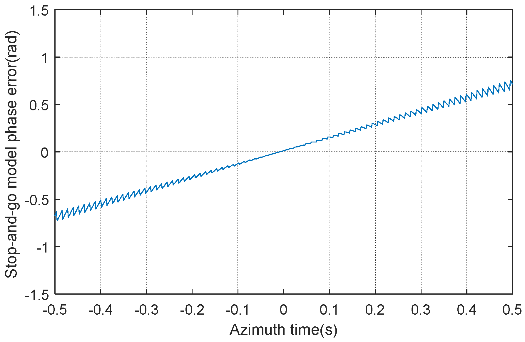
In order to verify the applicability of the stop-and-go approximation model in the staggered SAR, Figure 5 provides the phase error of the stop-and-go model versus the azimuth time. The parameters of the staggered SAR geometry were set to the same as those in

Table 1. Parameters of the simulated system and the two targets.

Parameter	Value
Carrier frequency	5.2 GHz
Orbit height	760 km
Off-nadir angle	23.3
Range bandwidth	180 MHz
Pulse duration	5 $\mu$s
Doppler band	1065 Hz
Velocity $[v_{Tx},v_{Ty},0]$	Target 1 [15 m/s, 10 m/s, 0]
	Target 2 [10 m/s, 5 m/s, 0]
Amplitude (roll, pitch, yaw)	Target 1 (5.2, 5.1, 2.6)
	Target 2 (5, 0, 0)
Period (roll, pitch, yaw)	Target 1 (25.6, 8.6, 18.2)
	Target 2 (26.4, 0, 0)

. The slant range error was obtained by calculating the difference between the round-trip slant ranges using the non-stop-and-go model and the stop-and-go model. As the azimuth time increased, the phase error also gradually accumulated in a linear trend. The overall error was less than $\pi /4$, indicating that the geometry configuration of the staggered SAR could match the stop-and-go approximation model.

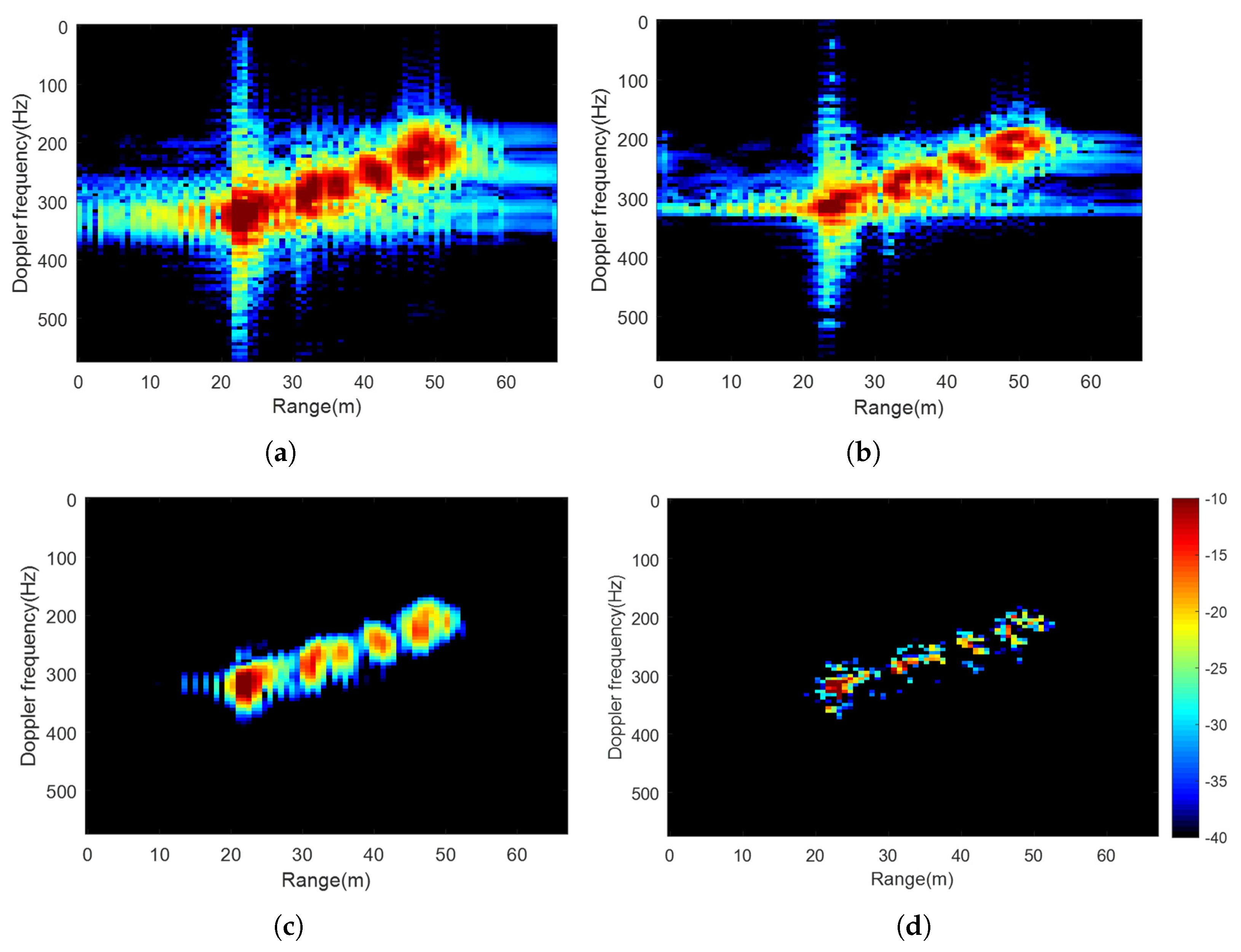
The ships moved at uniform speeds and underwent 3D rotations. Table 1 lists the parameters of the system and the targets. In order to verify the effectiveness of the modified BLU reconstruction in the proposed MBLCFD method, the defocused staggered SAR images of the two ship targets are provided in Figure 6 and Figure 7 using the original BLU method and the modified BLU method, respectively. Compared with the original BLU method, the modified BLU method could alleviate the high sidelobes spread for the whole azimuth. The amplitudes of the sidelobes were decreased, and the number of sidelobes was reduced, improving the performance of the azimuth ambiguity suppression. While the modified BLU method could alleviate the azimuth ambiguity, the images still suffered from severe defocusing and low resolution, which could be refocused using the subsequent ISAR processor. The zoomed-in versions around the targets are provided in Figure 8a and Figure 9a.

After combining the ISAR technology, Figure 8b–d and Figure 9b–d show the refocusing results of the two targets using the image-contrast-based autofocus (ICBA), the smoothed pseudo Winger–Ville distribution (SPWVD), and the proposed MBLCFD algorithm, respectively. Figure 8b and Figure 9b demonstrate much superior imaging performance than Figure 8a and Figure 9a since the ICBA adopts an optimization approach to estimate radial motion parameters. Even though the image quality is improved in Figure 8b,c and Figure 9b,c, the performance was limited due to the 3D rotation of the maritime target. Compared with the SPWVD, the proposed method based on a CTFD operated with the complex domain had the ability to deal with higher order phase signals and obtain superior time–frequency aggregation. The proposed MBLCFD reconstruction algorithm could reconstruct the scatters correctly and significantly improve the imaging performance of maritime targets in a staggered SAR, as shown in Figure 8d and Figure 9d.

Moreover, Figure 10 shows the imaging results under the low sea state. The movement of the target was smooth. For a smoothly moving target, the RD algorithm could obtain the focused image. Moreover, in this case, the RID technology could also be used. The azimuth signal could be considered as a quadratic phase signal. The imaging results verified the effectiveness of the proposed MBLCFD method under different sea states (different rotation degrees).

The SAR images for the whole scene with the proposed method are provided to demonstrate the algorithm’s effectiveness in suppressing the ambiguity along the azimuth. In the sub-image selection process, two rectangular windows with different sizes, with one relatively small and one relatively large, were utilized. The imaging results are shown in Figure 11. With a relatively small rectangular window, the ambiguity around the target could be suppressed, while the suppression performance of the ambiguity far away from the target was limited, as shown in Figure 11a. A relatively large rectangular window could suppress the high sidelobes spread along all of the azimuth.

It should be mentioned that the size of the rectangular window used during the sub-image selection in step 4 directly influenced the suppression of the azimuth ambiguity. Ideally, the size of the rectangular window will be the same as the observation time along the azimuth. In this way, the ambiguity in the whole azimuth can be alleviated. However, there will be multiple moving targets and stationary scenes in the scenario. If the size of the rectangular window is too large, the other targets and the stationary scene will be contained in the sub-image. The hybrid SAR/ISAR technique works well on the premise that each sub-image contains only one target. Moreover, a large sub-image will increase the energy of the remaining part of the image, which will be considered as noise or clutter, resulting in the degradation of the refocusing performance. If the size of the rectangular window is too small, the information of the moving target will be cut off. The ambiguity around the moving target could be suppressed effectively using ISAR processing. However, the ambiguity in the form of high sidelobes far away from the moving target could not be suppressed because it was not included in the sub-image. Thus, the size of the rectangular window should be set appropriately, with the aim to strike a balance between the scenario adaptability and the ambiguity performance.

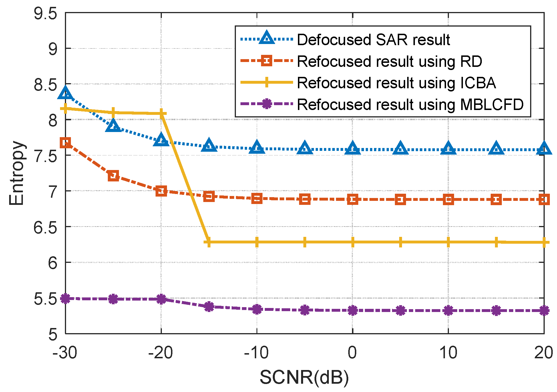
Figure 12 shows the entropy versus the signal clutter noise ratio (SCNR), illustrating that the MBLCFD had a high tolerance for the SCNR. The SCNR varied from −30 dB to 20 dB, with an interval of 5 dB. For the defocused SAR images, and the focused images using the RD method, the curve of entropy declined and flattens out gradually with the increase in the SCNR. The ICBA method was relatively sensitive to the SCNR when the SCNR was low. There was a noticeable decrease in entropy within the range of −20 dB to −15 dB. A potential explanation for this decrease is that the ICBA algorithm achieved image focusing by estimating the model parameters that maximized the image contrast. These model parameters were the polynomial coefficients of the focusing point phase term, which were derived without considering the noise and clutter components. The image entropy exhibited higher sensitivity to the changes in a low SCNR. Using the proposed MBLCFD, the performance improved as the SCNR increased. The smooth curve indicates a high tolerance for the SCNR.

The results in

Table 2. Reconstruction performance of maritime moving targets.

Performance		Defocused SAR Image	Refocused Image Using ICBA	Refocused Image Using SPWVD	Refocused Image Using MBLCFD
Target 1	MW (m)	4.59	2.02	2.89	1.25
	PLSR	−22.98	−25.19	−25.64	−26.01
	ISLR	−22.74	−23.51	−24.86	−25.54
	Entropy	7.5779	6.2833	6.1236	5.2802
Target 2	MW (m)	4.64	2.07	2.76	1.20
	PLSR	−22.02	−23.56	−24.73	−25.01
	ISLR	−22.45	−22.89	−23.63	−24.85
	Entropy	7.5800	6.0739	5.3970	5.1715

indicate that the proposed MBLCFD reconstruction algorithm had the smallest entropy and the smallest main lobe width (MW). The proposed algorithm had an improvement of about 3 dB for the ISLR and about 4 dB for the PSLR. Due to the expansion caused by the translation of the target, the resolution of SAR imaging was very low. The ICBA algorithm improved the resolution to some extent, but the effect was limited because of the time-varying Doppler frequency. The proposed MBLCFD reconstruction algorithm had the smallest entropy and the smallest main lobe width, indicating that superior image quality can be achieved.

Remark 6: The rotation parameters of the maritime targets, which significantly impacted the performance of refocusing, were determined by the sea states. In the presence of rough sea states, the nonlinear phase terms in the azimuth were increased, along with the range and Doppler migrations. This led to rapid changes in the instantaneous imaging projection planes (IPPs) and effective rotation vectors, which could not be effectively superimposed. As a result, the motion compensation became more complicated, and the image burring was aggravated.

5.2. Verification by Spaceborne SAR Data

To validate the feasibility of the proposed method, the equivalent staggered data were generated using Gaofen-3 spaceborne SAR data. The real spaceborne data were acquired by the GF-3 satellite over the city of Dalian in China. The signal was resampled and extracted using the fast linear PRI strategy. The generation of staggered equivalent data were proposed and analyzed in reference [25]. The raw data were resampled according to the sequence of variable PRIs with two-point interpolation, and blind ranges were considered after range compression. The large scene comprised a coastline with hills, villages, harbor, bridges, and multiple maritime moving targets.

The imaging result after the BLU and SAR processing is shown in Figure 13. The stationary scene on the coastline could be focused accurately, while the maritime targets were defocused due to the complex motion. Two maritime targets were selected and enlarged, as shown in Figure 14a and Figure 15a. Figure 14b–d and Figure 15b–d show the refocusing results of the two targets using the ICBA method, the SPWVD method, and the proposed MBLCFD algorithm based on the CTFD, respectively. The proposed MBLCFD outperformed the SPWVD-based reconstruction method in terms of time–frequency aggregation and cross-term suppression when processing the spaceborne SAR data. The proposed MBLCFD method improved the focusing performance, both in the range and azimuth dimensions. As shown in

Table 3. Reconstruction performance of maritime moving targets.

Performance		Defocused SAR Image	Refocused Image Using ICBA	Refocused Image Using SPWVD	Refocused Image Using MBLCFD
Target 1	Entropy	6.634	5.459	4.043	3.786
Target 2	Entropy	5.447	4.901	3.593	3.407

, the proposed MBLCFD reconstruction algorithm had the smallest image entropy compared with its rivals, showing better refocusing performance of maritime targets with 3D rotation.

Remark 7:The variable PRI and the target translation affected the image quality. The variable PRI caused nonuniform sampling along the azimuth. The nonuniform sampling and the target motion were coupled, degrading the image quality. However, in the proposed MBLCFD, the modified BLU method considers the target translational velocity, which can alleviate the couple of nonuniform sampling and the target motion. The velocity also allows SAR processing to compensate for the translational motion of the target. The complex-lag time–frequency distribution can ensure superior resolution without cross-terms. These factors improved the refocusing accuracy significantly.

6. Conclusions

This paper proposes a novel reconstruction method for maritime target imaging in a staggered SAR system. The geometric configurations and signal model for maritime moving targets were established in a staggered mode. The spectrum of the staggered SAR echo was derived by taking into account the variable PRI and complex maritime target motion. Derivations showed that the nonuniform sampling coupled with the target motion aggravated the spectrum aliasing along the azimuth, causing severe image defocusing. The proposed MBLCFD reconstruction algorithm offers a viable solution. Considering the velocity of the moving target, the BLU method was modified to resample the nonuniform sampling into a uniform grid. Precise SAR processing with the higher-order phase terms is performed to compensate for the curved orbit of the satellite and range–Doppler coupling terms. Based on a hybrid SAR/ISAR technique, the CTFD algorithm is exploited to refocus the maritime moving targets. Simulations and experiments demonstrated the effectiveness of the proposed MBLCFD algorithm in maritime target imaging for a staggered SAR. Compared with its rivals, the proposed MBLCFD reconstruction algorithm could provide superior imaging performance in terms of the PSLR, ISLR, and entropy.

References

- Ge, S.; Feng, D.; Song, S.; Wang, J.; Huang, X. Sparse Logistic Regression-Based One-Bit SAR Imaging. IEEE Trans. Geosci. Remote Sens. 2023, 61, 1–15. [Google Scholar] [CrossRef]
- Zhang, X.; Yang, P.; Wang, Y.; Shen, W.; Yang, J.; Wang, J.; Ye, K.; Zhou, M.; Sun, H. A Novel Multireceiver SAS RD Processor. IEEE Trans. Geosci. Remote Sens. 2024, 62, 1–11. [Google Scholar] [CrossRef]
- Xie, Z.; Wu, L.; Zhu, J.; Lops, M.; Huang, X.; Shankar, B. RIS-Aided Radar for Target Detection: Clutter Region Analysis and Joint Active-Passive Design. IEEE Trans. Geosci. Signal Process. 2024, 72, 1706–1723. [Google Scholar] [CrossRef]
- Zhu, J.; Song, Y.; Jiang, N.; Xie, Z.; Fan, C.; Huang, X. Enhanced Doppler Resolution and Sidelobe Suppression Performance for Golay Complementary Waveforms. Remote Sens. 2023, 15, 2452. [Google Scholar] [CrossRef]
- Zhang, S.; Xing, M.; Xia, X.; Guo, R.; Liu, Y.; Bao, Z. Robust Clutter Suppression and Moving Target Imaging Approach for Multichannel in Azimuth High-Resolution and Wide-Swath Synthetic Aperture Radar. IEEE Trans. Geosci. Remote Sens. 2015, 53, 687–709. [Google Scholar] [CrossRef]
- Huber, S.; de Almeida, F.Q.; Villano, M.; Younis, M.; Krieger, G.; Moreira, A. Tandem-L: A Technical Perspective on Future Spaceborne SAR Sensors for Earth Observation. IEEE Trans. Geosci. Remote Sens. 2018, 56, 4792–4807. [Google Scholar] [CrossRef]
- Moreira, A.; Krieger, G.; Hajnsek, I.; Papathanassiou, K.; Younis, M.; Lopez-Dekker, P.; Huber, S.; Villano, M.; Pardini, M.; Eineder, M.; et al. Tandem-L: A highly innovative bistatic SAR mission for global observation of dynamic processes on the earth’s surface. IEEE Geosci. Remote Sens. 2015, 3, 8–23. [Google Scholar] [CrossRef]
- Villano, M.; Pinheiro, M.; Krieger, G.; Moreira, A.; Rosen, P.A.; Hensley, S. Gapless imaging with the NASA-ISRO SAR (NISAR) mission: Challenges and opportunities of staggered SAR. In Proceedings of the EUSAR, Aachen, Germany, 5–7 June 2018; pp. 1–6. [Google Scholar]
- Villano, M.; Krieger, G.; Moreira, A. Staggered-SAR: A New Concept for High-Resolution Wide-Swath Imaging. In Proceedings of the IEEE Gold Remote Sensing Conference, Rome, Italy, 4–5 June 2012; pp. 1–3. [Google Scholar]
- Krieger, G.; Gebert, N.; Younis, M.; Bordoni, F.; Patyuchenko, A.; Moreira, A. Advanced concepts for ultra-wide-swath SAR imaging. In Proceedings of the EUSAR, Friedrichshafen, Germany, 2–5 June 2008. [Google Scholar]
- Freeman, A.; Krieger, G.; Rosen, P.; Younis, M.; Johnson, W.T.K.; Huber, S.; Jordan, R.; Moreira, A. SweepSAR: Beam-forming on receive using a reflector-phased array feed combination for spaceborne SAR. In Proceedings of the IEEE Radar Conference, Pasadena, CA, USA, 4–8 May 2009. [Google Scholar]
- Villano, M.; Krieger, G.; Moreira, A. Staggered SAR: High-resolution wide-swath imaging by continuous PRI variation. IEEE Trans. Geosci. Remote Sens. 2014, 52, 4462–4479. [Google Scholar] [CrossRef]
- Wang, X.; Wang, R.; Deng, Y.; Wang, W.; Li, N. SAR signal recovery and reconstruction in staggered mode with low oversampling factors. IEEE Geosci. Remote Sens. Lett. 2018, 15, 704–708. [Google Scholar] [CrossRef]
- Luo, X.; Wang, R.; Xu, W.; Deng, Y.; Guo, L. Modification of multichannel reconstruction algorithm on the SAR with linear variation of PRI. IEEE J. Sel. Top. Appl. Earth Observ. Remote Sens. 2014, 7, 3050–3059. [Google Scholar] [CrossRef]
- Zhou, Z.; Deng, Y.; Wang, W.; Jia, X.; Wang, R. Linear Bayesian approaches for low-oversampled stepwise staggered SAR data. IEEE Trans. Geosci. Remote Sens. 2021, 60, 5206123. [Google Scholar] [CrossRef]
- Liu, Z.; Liao, X.; Wu, J. Image reconstruction for low-oversampled staggered SAR via HDM-FISTA. IEEE Trans. Geosci. Remote Sens. 2021, 60, 5204514. [Google Scholar] [CrossRef]
- Ustalli, N.; Villano, M. High-Resolution Wide-Swath Ambiguous Synthetic Aperture Radar Modes for Ship Monitoring. Remote Sens. 2022, 14, 3102. [Google Scholar] [CrossRef]
- Ustalli, N.; Krieger, G.; Villano, M. A low-power, ambiguous synthetic aperture radar concept for continuous ship monitoring. IEEE J. Sel. Top. Appl. Earth Obs. Remote Sens. 2022, 15, 1244–1255. [Google Scholar] [CrossRef]
- Martorella, M.; Giusti, E.; Berizzi, F.; Bacci, A.; Mese, E.D. ISAR based technique for refocusing non-copperative targets in SAR images. IET Radar Sonar Navigat. 2012, 6, 332–340. [Google Scholar] [CrossRef]
- Long, T.; Hu, C.; Ding, Z.; Dong, X.; Tian, W.; Zeng, T. GEO SAR system analysis and design. In Geosynchronous SAR: System and Signal Processing; Springer: Singapore, 2018; pp. 27–76. [Google Scholar]
- Liu, Z.; Jiang, Y. A Novel Doppler Frequency Model and Imaging Procedure Analysis for Bistatic ISAR Configuration With Shorebase Transmitter and Shipborne Receiver. IEEE J. Sel. Top. Appl. Earth Observ. Remote Sens. 2016, 9, 2989–3000. [Google Scholar] [CrossRef]
- Hu, C.; Long, T.; Liu, Z.; Zeng, T.; Tian, Y. An Improved Frequency Domain Focusing Method in Geosynchronous SAR. IEEE Trans. Geosci. Remote Sens. 2014, 52, 5514–5528. [Google Scholar]
- Munoz-Ferreras, J.M.; Perez-Martinez, F. On the Doppler Spreading Effect for the Range-Instantaneous-Doppler Technique in Inverse Synthetic Aperture Radar Imagery. IEEE Geosci. Remote Sens. Lett. 2010, 7, 180–184. [Google Scholar] [CrossRef]
- Zaric, N.; Orovic, I.; Stanković, S. Robust Time-frequency Distributions with complex-lag Argument. EURASIP J. Adv. Signal Process. 2010, 2010, 879874. [Google Scholar] [CrossRef]
- Villano, M. Staggered Synthetic Aperture Radar. Ph.D. Thesis, Deutsches Zentrum für Luft- und Raumfahrt (DLR) Oberpfaffenhofen, Bavaria, Germany, 2016. [Google Scholar]
Figure 1.
Geometry of staggered SAR system for maritime moving target.
Figure 2.
Spectrum analysis in azimuth for staggered mode. Top: stationary target. Bottom: moving target.
Figure 3.
Flowchart of the proposed MBLCFD reconstruction algorithm for maritime moving targets.
Figure 4.
The PRI sequence of the fast linear variation strategy. (a) The PRI trend. (b) The location of the blind ranges. (c) The percentage of the lost pulses.
Figure 5.
Stop-and-go approximation model phase error versus azimuth time.
Figure 6.
Simulated target 1. (a) Defocused staggered SAR image using original BLU method. (b) Defocused staggered SAR image using modified BLU method.
Figure 7.
Simulated target 2. (a) Defocused staggered SAR image using original BLU method. (b) Defocused staggered SAR image using modified BLU method.
Figure 8.
Simulated target 1. (a) Zoomed-in SAR defocused image, and the refocused images (b) using the ICBA method, (c) using SPWVD method, and (d) using proposed MBLCFD method.
Figure 9.
Simulated target 2. (a) Zoomed-in defocused SAR image, and the refocused images (b) using ICBA method, (c) using SPWVD method, and (d) using proposed MBLCFD method.
Figure 10.
Simulated target under low sea state. (a) Zoomed-in defocused SAR image, and refocused images (b) using RD algorithm, (c) using ICBA, and (d) using proposed MBLCFD method.
Figure 11.
Refocused staggered SAR image. (a) Operated with a relatively small rectangular window in sub-image selection. (b) Operated with a relatively large rectangular window in sub-image selection.
Figure 12.
The entropy versus the SCNR.
Figure 13.
Imaging results of large scene.
Figure 14.
Actual target 1 (AT1). (a) Results of the defocused SAR image, and the refocused images using (b) the ICBA method, (c) the SPWVD method, and (d) the proposed method.
Figure 15.
Actual target 2 (AT1). (a) Results of the defocused SAR image, and the refocused images using (b) the ICBA method, (c) the SPWVD method, and (d) the proposed method.