Land Cover Characterization and Mapping of South America for the Year 2010 Using Landsat 30 m Satellite Data

Abstract
: Detailed and accurate land cover and land cover change information is needed for South America because the continent is in constant flux, experiencing some of the highest rates of land cover change and forest loss in the world. The land cover data available for the entire continent are too coarse (250 m to 1 km) for resource managers, government and non-government organizations, and Earth scientists to develop conservation strategies, formulate resource management options, and monitor land cover dynamics. We used Landsat 30 m satellite data of 2010 and prepared the land cover database of South America using state-of-the-science remote sensing techniques. We produced regionally consistent and locally relevant land cover information by processing a large volume of data covering the entire continent. Our analysis revealed that in 2010, 50% of South America was covered by forests, 2.5% was covered by water, and 0.02% was covered by snow and ice. The percent forest area of South America varies from 9.5% in Uruguay to 96.5% in French Guiana. We used very high resolution (<5 m) satellite data to validate the land cover product. The overall accuracy of the 2010 South American 30-m land cover map is 89% with a Kappa coefficient of 79%. Accuracy of barren areas needs to improve possibly using multi-temporal Landsat data. An update of land cover and change database of South America with additional land cover classes is needed. The results from this study are useful for developing resource management strategies, formulating biodiversity conservation strategies, and regular land cover monitoring and forecasting.1. Introduction
Anthropogenic land use and land cover change, occurring at unprecedented rates, magnitudes, and spatial scales [1,2], is increasingly affecting the biophysics, biogeochemistry, and biogeography of the Earth’s surface and atmosphere with far-reaching consequences to human well-being [3]. However, our scientific understanding of the distribution and dynamics of land use and land cover change is limited [4]. Accurate, reliable, and timely information on historical and contemporary distribution and dynamics of land cover is essential for land change research and for biodiversity conservation [5–7]. Such information is also needed for monitoring, understanding, and predicting the effects of human-nature interactions [8–10].
The global change community is placing greater emphasis on developing these datasets at multiple spatial, thematic, and temporal scales [11–14]. For example, land cover is one of the 50 Essential Climate Variables (ECVs) identified by the Committee on Earth Observation Satellites (CEOS) that are “technically and economically feasible for systematic observation”. The Global Terrestrial Observing System (GTOS) further identified land cover as one of the five highest priority ECVs along with biomass, glacier and ice caps, soil moisture, and permafrost. Similarly, generating land cover ECVs is now recognized as an official task of the Group on Earth Observations (GEO). At the same time, it is becoming increasingly common and important to produce a better resolution global land cover database and integrate product validation into initial research design, perform validation, and distribute statistically validated data.
Timely and accurate land cover information is especially needed in South America because the region is in constant flux, experiencing some of the highest rates of land cover change and forest loss in the world [15]. South America has the largest area of tropical forests in the world, the greatest amount of biodiversity, and a large reservoir of above and below ground carbon stock, but the forest is under threat from anthropogenic forces [16]. Specifically, extensive areas of the Amazon rain forest and the seasonally dry forests of Brazil, Bolivia, Paraguay, and Argentina are undergoing deforestation and conversion to agriculture [17,18]. The forest clearing will likely continue for agriculture and harvesting for commercial use, causing further land use and land cover change in the coming decades [19]. Such widespread land cover change is causing habitat degradation and releasing vast stores of carbon dioxide into the atmosphere, further exacerbating the impacts of global climate change to nature and society [20,21]. Quantifying the contribution of terrestrial ecosystems to global and regional carbon flux requires timely and accurate land cover products and information [22] at the highest resolution possible.
Although several land cover databases exist for South America, they have limitations. For example, previous land cover mapping performed as part of global land cover assessments were derived from coarse spatial resolution (250 m–8 km) satellite data [8,9,19,23–31]. Coarse land cover products do not provide sufficient spatial details for land cover change studies for biodiversity conservation and resource management at a national or sub-national scale. Additionally, coarse spatial resolution mapping frequently represents composite spectral responses from multiple land cover types (i.e., mixed pixels), resulting in map inaccuracies [32]. Recently, global land cover [33] and global percent tree cover [18] were mapped using Landsat 30 m but these maps do not provide spatial and thematic details needed for continental applications. National land cover data are available but they are spatially and temporarily inconsistent across the continent.
The overall goal of this paper is to prepare a validated land cover database of South America for the year 2010 using Landsat 30 m imagery. The regionally tuned image classification approach and training data were selected based on land cover variability and complexity of South America. The land cover map was validated using a very high resolution (<5 m) validation dataset [3]. A confusion matrix was constructed and class accuracies were reported. This 30 m spatial resolution South America land cover database provides resource managers, government and non-government organizations, and Earth scientists with accurate and reliable information for developing conservation strategies, biodiversity loss mitigation efforts, and monitoring of land cover dynamics.
2. Study Area
The study area includes the entire South American continent. South America extends from approximately 12°N to 56°S latitude, occupies 17.8 million km2, and has several distinct geologic and biogeographic regions with varying land cover types. For example, the Amazon rain forest, the largest tropical rain forest and one of the most bio-diverse ecosystems in the world, extends across much of the north-central region. The Andes Mountains, the longest continental mountain range in the world, extend from north to south along the western coast. The Atacama Desert, one of the driest hot deserts in the world, is situated along the west coast between the Andes Mountains and Pacific Ocean. The Pantanal, one of the world’s largest tropical wetlands, is located in central South America, mostly in Brazil. The Pampas, an extensive and relatively flat grassland area, makes up the central and western portions of Argentina. The Patagonian steppe begins to the south of the Pampas and extends west from the Andes to the Atlantic coast.
3. Methods
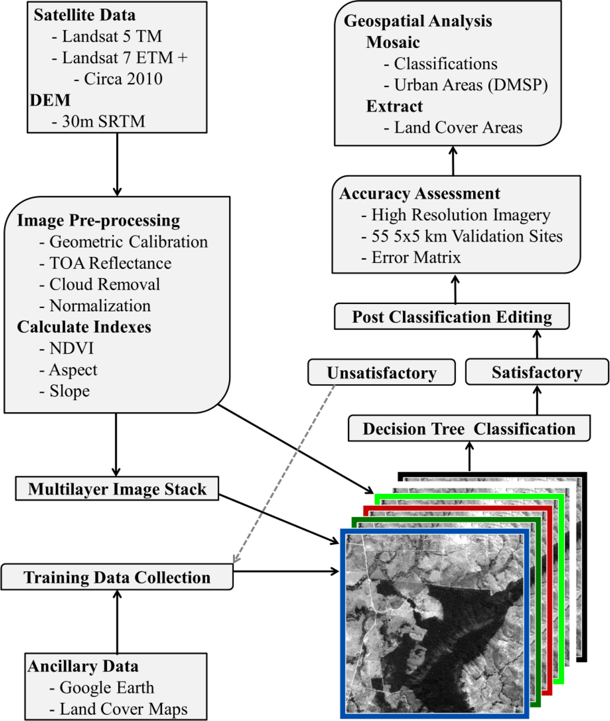
Figure 1 illustrates the methodological framework of this research. We classified Landsat 5 Thematic Mapper (TM) and Landsat 7 Enhanced Thematic Mapper Plus (ETM+) satellite data for 2010 using a decision tree classification approach. Normalized Difference Vegetation Index (NDVI) and the Shuttle Radar Topography Mission (SRTM) Digital Elevation Model data at 30 m spatial resolution were used as independent variables. The SRTM elevation data were obtained on a near-global scale in 2000 [34] and acquired from the U.S. Geological Survey Earth Resources Observation and Science (EROS) Center. The results were validated using 55, 5 × 5 km2 sample blocks and very high resolution classification results.
3.1. Land Cover Classification System and Legend
We mapped five discrete land cover classes: trees, open water, barren, perennial snow/ice, and other vegetation. Additionally, clouds and shadows were classified separately. Similar to [19], we used radiance calibrated “stable lights” data from the Defense Meteorological Satellite Program (DMSP) to delineate urban areas [35]. Land cover classes were defined using the Land Cover Classification System (LCCS), which is “a comprehensive methodology for description, characterization, classification, and comparison of most land cover features identified anywhere in the world, at any scale or level of detail” [36]. Definitions, delineation criteria, and interpretation guidelines used in this study are given below.
Forests are defined as woody perennial plants, 3 m or greater in height. This category includes evergreen and/or deciduous, broad-leaved and/or needle-leaved, and mixed forests found in terrestrial, aquatic, or regularly flooded locations as well as trees found in both natural and cultivated/managed situations. For example, trees located in farms, orchards, and landscaping that satisfied the 3 m minimum criteria were classified as trees. Stunted or young trees and shrubbery that are less than 3 m tall were classified as other vegetation. Trees were delineated around the edge of the tree crowns. If tree crowns coalesce, then trees were collected around the outermost edge of the crowns.
Water is defined as flowing or standing water bodies in aquatic or regularly flooded locations. Water includes natural water bodies such as streams, rivers, lakes, ponds, oceans, and swamps / marshes. Water also includes artificial water bodies such as ditches, canals, impounded stream courses, and reservoirs. However, inundated vegetation such as trees, shrubs, or grass growing in a water body are classified as trees or other vegetation wherever these features obscure the surface of the water body. Water is delineated at the shoreline of the water body. Dynamic water bodies such as tidal and flood waters were classified as captured in the source imagery.
Barren is defined as land surface lacking vegetation or water bodies. This class includes natural bare surfaces such as bedrock, bare soil, hard pans, sand/gravel bars, beaches, loose and shifting sand, exposed rock, glacial debris, and dry salt flats. Barren areas include artificial impervious surfaces such as strip mines, quarries, gravel pits, and other accumulations of earthen materials. Barren includes both consolidated and unconsolidated surfaces. Recently tilled agricultural fields, recently burned vegetation, recently flood-scoured vegetation, and clear-cut trees are classified as other vegetation because other vegetation is expected to grow back in a relatively short time period.
Urban is defined as artificial impervious surfaces such as paved and unpaved roads and other transportation surfaces; commercial, residential, or industrial structures; and roof tops. Urban areas can often be visually detected in low-resolution satellite images; however, due to their context and location, they are problematic to extract from the digital data because their spectral signature is similar to bare soil. Similar to [19], we used radiance calibrated “stable lights” data from the DMSP to locate the major urban areas [35]. The DMSP data were resampled to 30 m and overlaid on the 30 m land cover mosaic to ensure adequate colocation. No substantial misalignment was apparent.
Other Vegetation is defined as woody perennial plants less than 3 m in height and all non-woody shrubs, forbs, herbaceous vegetation (graminoids or non-graminoids), lichens, and mosses. As explained under the barren class, recently flood-scoured vegetation, recently burned vegetation, and recently clear-cut trees were classified as other vegetation. Similarly, vine crops such as grapes or hops were classified as other vegetation. Other vegetation classes were delineated where vegetation cover is apparent and water or trees are absent.
Perennial Snow and Ice is defined as frozen water that does not melt during any time of the year. Perennial snow and ice areas include snow pack, glaciers, frozen lakes, rivers, and ponds.
Clouds and Shadows were classified as a separate class where they prevented delineation of land cover classes. Shadows may have been caused by clouds, trees, infrastructure, or terrain (cliffs, mountains, raised buildings, or hills).
3.2. Data and Pre-Processing
All the Landsat 7 and Landsat 5 imagery available at USGS EROS for South America was downloaded in L1T format. The data were acquired for the growing season for 2010 spanning from November 2009 to February 2010. Major pre-processing steps include geometric correction, calibration to top-of-atmosphere (TOA) reflectance, cloud removal, MODIS base normalization, and per-pixel compositing. Although most of the Landsat L1T products were within ±1 pixel geometric accuracy, a few scenes were less accurate. Thus, it was necessary to check the geometric accuracy and correct the problem. We used Global Land Survey (GLS) 2000 data to check the accuracy. If the accuracy was more than ±1 pixel, Landsat images were resampled using ground control points (GCPs) selected from GLS 2000 data and the nearest neighbor resampling technique.
Each image was normalized for variation in solar angle and Earth-Sun distance by converting the digital number values to TOA reflectance. This is a two-step process: conversion of Digital Numbers (DNs) to radiance values using the bias and gain values specific to the individual Landsat scene and conversion of radiance values to TOA reflectance. For each scene, information on the distance between the Sun and Earth in astronomical units, the day of the year (Julian date), and solar zenith angle is needed and can be obtained from the Landsat 7 Science Users Handbook [37].
Radiometric normalization of Landsat was performed using dark-object subtraction (DOS) methods to remove errors associated with sensor calibration changes, differences in illumination and observation angles, variation in atmospheric effects, and phenological variations [38]. Two types of intact and uncontaminated forest pixels were used for DOS: pixels selected from forest/non-forest maps produced from MODIS satellite data, and pixels with Landsat band 6 thermal brightness temperature values greater than or equal to 19 degrees Celsius [38].
The per-pixel image composite was performed from the pre-processed data. The first step involved selection of best pixels out of seasonal stacks considering cloud, cloud shadows, and Scan Line Corrector (SLC) off data among others. For example, cloud removal steps include calculation of a simple cloud likelihood score for each input pixel. The selection was based on the Landsat band 6 brightness temperature of the pixel. The minimum value of the cloud likelihood score at each location was used to select a cloud likelihood threshold for the pixel. The output is the per-band median of the pixels whose cloud likelihood scores fell below that threshold. The next step was to select a median TOA reflectance and cloud likelihood threshold for each pixel of the growing season to prepare a seasonal mosaic. Impact of SLC off and cloud/shadows effect was not removed completely on the final mosaic. Finally, the resulting TOA reflectance estimates were rescaled to the 8-bit integer range. To manage the data volume and facilitate image classification, 12 mosaics, or tiles, were prepared covering all of South America.
All the pre-processing steps were performed using an open source MapPy python library that is Windows compatible. MapPy depends on various third-party packages and modules including, Geospatial Data Abstraction Library (GDAL), and NumPy [39]. We used MapPy, an automated approach, to perform image processing (unzip Landsat download, stack/composite, mask, mosaic, TOAR calibration, cloud detecting, Cloud Filling, and calibrate Landsat to MODIS Surface Reflectance), and generate indices (e.g., NDVI and MSAVI). The package, available freely upon request could also perform feature extraction, principal component analysis, and image classification using random forests and support vector machine.
3.3. Image Classification
A supervised decision-tree classification approach (Random Forest) was used for image classification. The random forest classifier uses bagging to form an ensemble of classification. It consists of a combination of tree classifiers and each tree casts a vote for the most popular class to classify an input vector[40]. A decision-tree classification is a procedure that recursively partitions a dataset into smaller subdivisions on the basis of a set of tests defined at each branch or node in the tree. The tree is composed of a root node (formed from training data), a set of internal nodes (splits), and a set of terminal nodes (leaves) [41,42]. The quality of the training site database strongly influences the quality of classification results [27]. Training classes were generated by selecting a sample of pixels for each land cover class (e.g., forest) from several data sources: Landsat imagery, high-resolution imagery, and land cover maps. Landsat spectral bands 3, 4, 5, and 7, NDVI, and elevation data and derivatives (i.e., Slope, and Aspect) were independent variables for categorical classification. Only the composite of growing season Landsat data and NDVI derived from the composite was analyzed. Training data collection and classification were performed independently for each tile while paying special attention to edge mismatch. Urban areas were not mapped using Landsat but were obtained from the DMSP Operational Linescan System (OLS) nighttime stable light (NTL) datasets [43]. This freely available dataset consists of average visible and cloud free stable lights. NASA researchers have used these nighttime lights images to map urban areas[35,44].
In areas where land cover features were misclassified and classification output was considered unsatisfactory, we added training data, redeveloped the decision tree models, and reapplied the models to the respective predictor variables. Once classification output was considered satisfactory, post-classification refinement, where apparent misclassified pixels were manually reclassified by the interpreter to the correct class label, was performed to eliminate apparent misclassification errors. Finally, all classified imagery was mosaicked to produce a single thematic land cover map for all of South America. The benefits of this approach are (i) it is a semi-automated approach with minimal input from the interpreter, and (ii) the analysis could be completed in a shorter time frame compared to traditional classification approach.
3.4. Accuracy Assessment
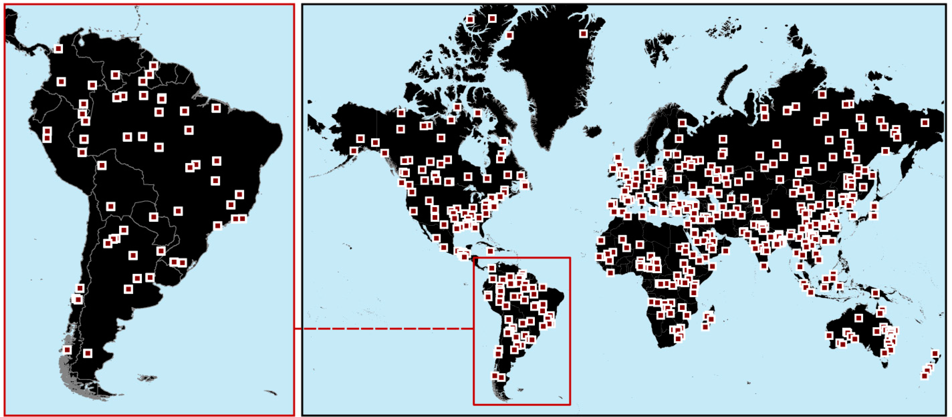
Olofsson et al. [45] proposed a global sample of 500 validation sites (Figure 2), with each site 5 × 5 km in area. These global validation sites were selected using a stratified random sampling approach. A total of 21 strata were used based on modified Köppen Climate/Vegetation classification and population density. The ultimate goal is to develop these validation sites as permanent plots that will be periodically/iteratively updated and used for validating a variety of land cover products. Furthermore, these global samples may be augmented to address specific accuracy objectives based on a target land cover map or geographic region [46].
For this study, we used all 55 global sampling blocks that are located in South America to validate its land cover (Figure 2). These 55 sites statistically represent the diverse land cover types of South America including undisturbed rain forest, mix of rain forest and cleared forest for pasture, gallery forests, savannas, woodlands, grasslands, exposed rocks, roads, sands, urban areas, croplands, and water bodies. However, these sampling blocks were not designed specifically to validate land cover of South America.
Very high resolution multispectral and panchromatic satellite data obtained from the National Geospatial Agency (NGA) Web-based Access and Retrieval Portal (WARP) were used as a reference data source to validate the Landsat 30 m land cover product. Data types included WorldView-1, WorldView-2, IKONOS, QuickBird, OrbView-3, and GeoEye-1. These data were acquired at the growing season (November 2009–February 2010), same season as Landsat satellite data acquisition. However, target imagery acquisition was not always possible due to the unavailability of data or cloud and shadow. Because of this, a small fraction (less than 5%) of the data was collected from outside the growing season or from non-target years. Resolution of multispectral data at optimal nadir imaging geometry ranges from 1.65 m for the GeoEye sensor to 4 m for OrbView-3, and resolution of the panchromatic data ranges from 0.41 m for GeoEye to 1 m for OrbView-3. These various resolution data were resampled to 2 m and classified using a decision tree classifier. Consistent with our land cover classes, the reference data land cover classes are defined using LCCS.
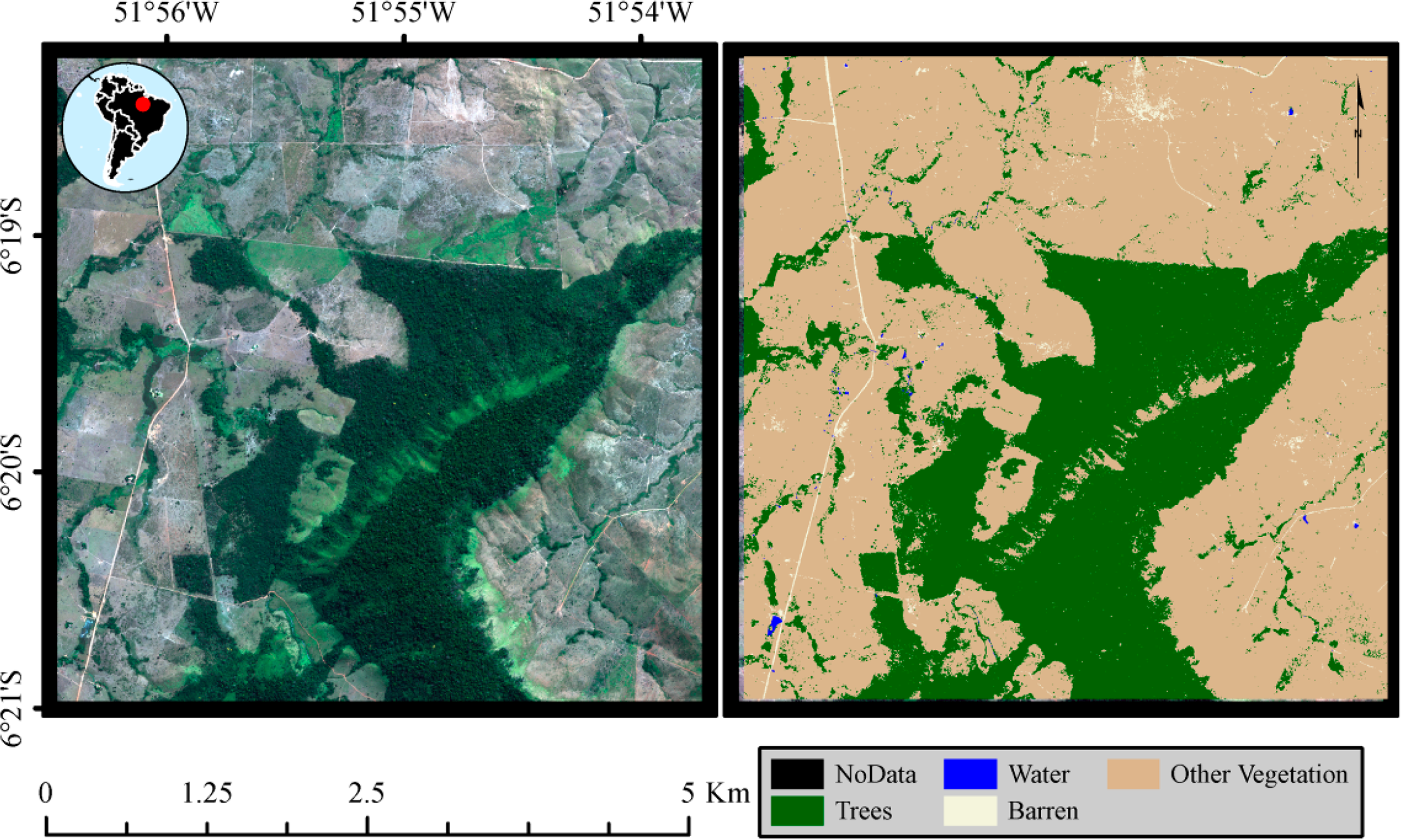
Pre-processing steps involved orthorectification and sub-setting of imagery prior to image classification. Orthorectification was performed using Rational Polynomial Coefficient (RPC) modeled sensor orientation data supplied with the image data and Advanced Spaceborne Thermal Emission and Reflection Radiometer (ASTER) Global Digital Elevation Model 2 (GDEM v2). We used a similar classification approach as Landsat classification (Figure 1) to produce four discrete land cover classes: trees, open water, barren, and other vegetation (Figure 3). Training data were collected visually using ERDAS Imagine software. Ideally, it is suggested to check the accuracy of reference datasets from field visits and in-situ measurements. However, it was not practical to conduct a field survey of all 55 sites for this study. To minimize these errors, we organized a week-long peer review workshop involving three interpreters to check the quality of classification results in each 1 km × 1 km regularly spaced blocks. Based on consensus agreement, errors were identified and removed through iterative classification and editing.
All very high resolution reference images in the 55 sample blocks were resampled from 2 m to 30 m using the class majority rule. In total, approximately 1.4 million reference points were used for the South America land cover accuracy assessment. Finally, a confusion matrix was constructed to cross tabulate the observed data with the reference data [47].
3.5. Areal Statistics
Land cover areas were calculated for all countries in South America. First, the land cover mosaic was transformed to Albers Equal Area projection. A geospatial vector dataset containing South America’s administrative country boundaries was used to tabulate land cover areas per country.
The analysis took six months for one expert to acquire the data, perform pre-processing, and perform image classification. Preparation of the validation database took approximately six months for two image analysts. Deskstop computers and a server with 30 TB of diskspace were used for the analysis.
4. Results and Discussion
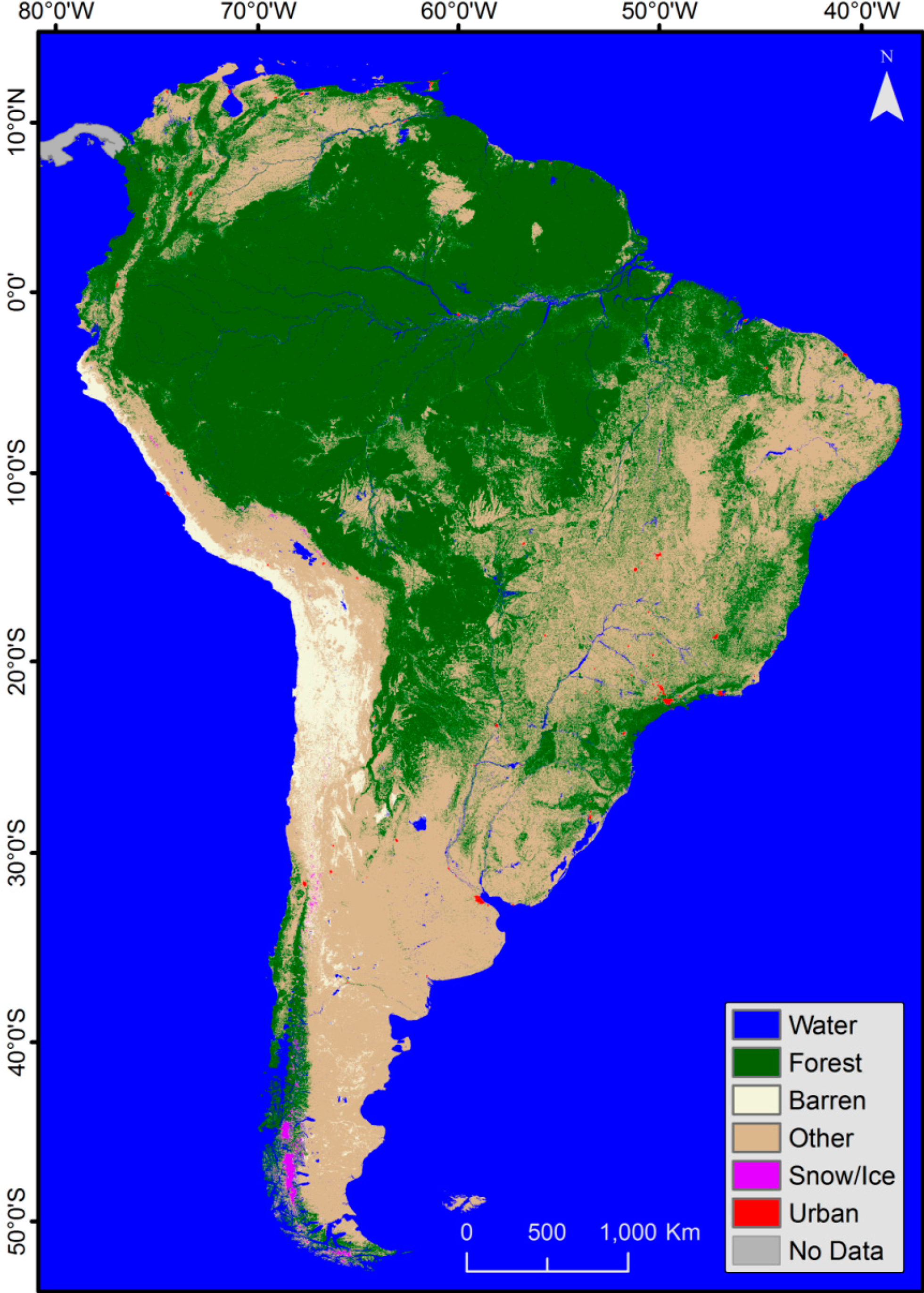
We prepared an accurate and contemporary wall-to-wall map depicting South America’s land cover (Figure 4) at 30 m spatial resolution [48]. The database reveals the status of land cover in South America for 2010 at a resolution finer than previous mapping efforts. Previous land cover datasets were prepared using coarser spatial resolution satellite data ranging from 250 m to 1 km. According to our estimate, 50% of South America is covered by forests, approximately 2.5% is covered by water, and only 0.02% is covered by snow and ice.
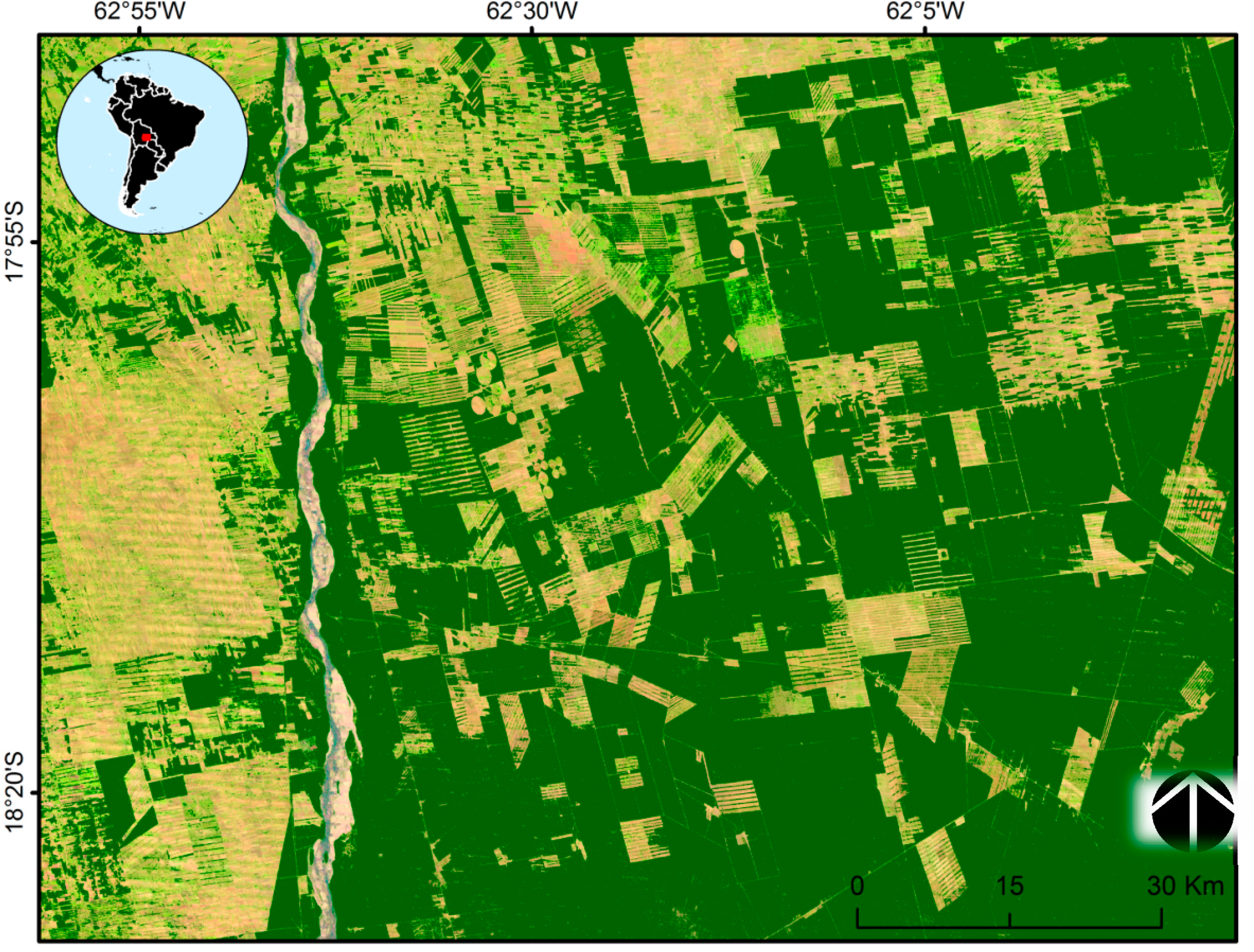
The 30 m resolution is suitable for national and sub-national applications. The 30 m land cover product can be used for local-scale resource management (Figure 5). For example, several national and sub-national land cover initiatives have been using 30 m or similar resolution satellite data for land cover mapping and monitoring [49,50]. The global change science community benefits from these datasets because 30 m resolution data (i) permits detection of land change at the scale of most human activity; (ii) offers increased flexibility for environmental model parameterization; (iii) provides spatial information content that is better than existing global land cover datasets; (iv) supports many GEO tasks and activities, including GEO Agriculture, Forest Carbon Tracking, the Biodiversity Observation Network, and the Land Cover Task; and (v) provides globally consistent and locally relevant information. The database fulfills the requirement of resource managers as well as that of the global change research community.
With this new database, we calculated the areal extent of five land cover classes for each country of South America for 2010 (Table 1). These data can serve resource managers and scientists with information for developing conservation strategies, biodiversity loss mitigation efforts, and monitoring land cover and climate dynamics.
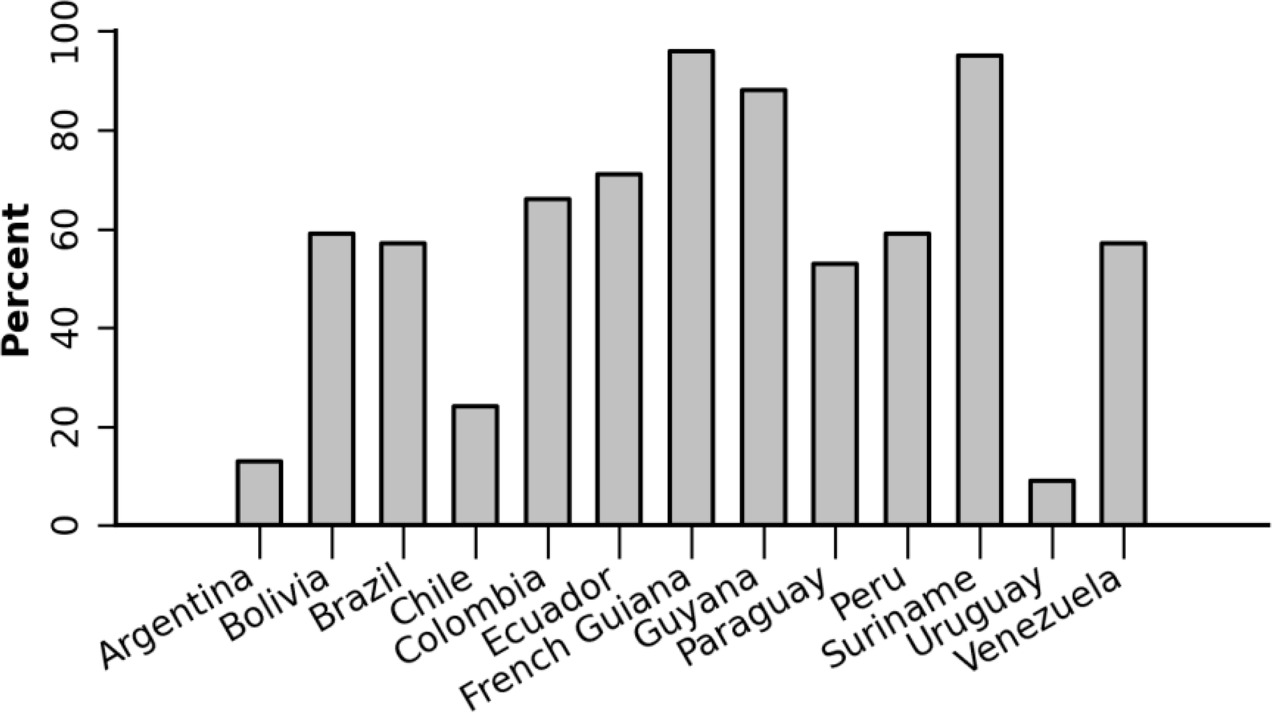
Percentage forest area of South American countries varies from 9.5% in Uruguay to 96.5% in French Guiana (Figure 6). South American forests form an important part of the world’s forests, particularly tropical rain forest. The tropical rain forest in South America is mainly concentrated in the Amazon River Basin. Outside the Amazon, tropical rain forests are found in coastal Brazil and in northern and western South America extending from Peru to Venezuela.
An accuracy assessment performed on the 2010 South America 30 m land cover map indicated high classification accuracy, with an overall accuracy of 89% and Kappa of 79% (Table 2). Forest, water, and other vegetation were classified with high accuracies. However, barren class had the lowest producer’s and user’s accuracies. The timing of the data acquisition may have caused the low accuracy for the barren class. The Landsat data used for land cover mapping and very high resolution satellite data used for reference data were not consistently acquired at the same time of the growing year. Land cover conversion and phenological changes that might have occurred during these time differences complicate interpretation and comparison. For example, cleared forest in tropical areas may change to shrubs and grasses within a few weeks or months. To improve classification accuracy of barren areas, multi-temporal data are needed. The accuracy of the snow and ice class was not assessed because of a lack of reference data.
Input Landsat data limitations impacted the land cover classifications output for South America. Cloud cover, although minimal in area (5668 km2), was persistent in some areas throughout the study area and prevented land cover mapping of target classes. Additionally, an anomaly of the Landsat 7 ETM+ Scan Line Corrector (SLC) in 2003 resulted in 22% data loss per scene. This data loss appears in the form of wedge-shaped gaps widening from the scene center toward the scene edge. These data gaps were “filled” with supplementary imagery; however, issues with differing capture dates of the Landsat 7 ETM+ SLC-off imagery and the supplementary data caused problems with land cover characterization is some areas.
5. Conclusions
We produced a land cover database of South America for the year 2010 using Landsat 30 m spatial resolution satellite data. Though several land cover databases for South America existed prior to our study, they were derived from coarse resolution imagery ranging from 250 m to 1 km. Our database provides information with details relevant at local and national applications. Mapping at 30 m spatial resolution was made possible due to availability of free Landsat satellite data, and advancement in image processing and computing resources. For example, we used all growing season data of 2010, automated image pre-processing techniques, semi-automated image classification approach, and servers and workstations to analyze the data. Until recently, mapping of the entire South American continent at this resolution was impractical mainly due to data costs, data volume, small image extent, haze and cloudiness, and sporadic acquisitions [51].
Based on the analysis of remotely sensed satellite observations and digital image classification techniques, our investigation provides contemporary and accurate data regarding South America’s land cover extent and spatial distribution for 2010. Our analysis revealed that in 2010, 50% of South America is covered by forests, 2.5% is covered by water, and 0.02% is covered by snow and ice. The percent forest area of South America varies from 9.5% in Uruguay to 96.5% in French Guiana. We used very high resolution (<5 m) satellite data to validate the land cover product. The overall accuracy of the 2010 South America 30 m land cover map is 89% with a Kappa coefficient of 79%. The results from this study are useful for developing biodiversity conservation strategies and future land cover monitoring and prediction.
The pre-processed Landsat data and land cover product generated from this research is freely available from the USGS. The national mapping agencies, regional/international organizations, and researchers can benefit from our analysis in two distinct ways: further analysis could be performed using this baseline land cover data and pre-processed satellite data. The pre-processed data could be used to perform detailed land cover analysis at national or local scales. Similarly, our land cover data could be used to produce additional land cover classes utilizing pre-processed Landsat data and a hierarchical classification approach. For example, the forest class could be sub-divided into evergreen and deciduous forests. Methods developed and used in this study have two major advantages: the method is a semi-automated approach with minimal input from the interpreter, and the analysis can be completed in a shorter time frame compared to a traditional classification approach.
In the future, additional land cover classes such as cropland, grassland, and wetlands need to be included in the classification. Accuracy of barren areas needs to be improved, possibly using multi-temporal Landsat data. A periodic update (e.g., every 3–5 years) of land cover and validation data is also needed.
Acknowledgments
We would like to thank Thomas Adamson for editing the manuscript. We would also like to thank four anonymous reviewers for their insightful comments and suggestions. Any use of trade, firm, or product names is for descriptive purposes only and does not imply endorsement by the U.S. Government.
Author Contributions
Chandra Giri and Jordan Long analyzed the data and prepared the manuscript.
Conflicts of Interest
The authors declare no conflict of interest.
References
- Turner, B.; Meyer, W.B.; Skole, D.L. Global land-use/land-cover change: Towards an integrated study. Ambio. Stockholm 1994, 23, 91–91. [Google Scholar]
- Giri, C.P. Brief overview of remote. In Remote Sensing of Land Use and Land Cover: Principles and Applications; CRC Press: Boca Raton, FL, USA, 2012; Volume 8, p. 1. [Google Scholar]
- Giri, C.; Pengra, B.; Long, J.; Loveland, T.R. Next generation of global land cover characterization, mapping, and monitoring. Int J Appl Earth Obs 2013, 25, 30–37. [Google Scholar]
- Foody, G.M. Status of land cover classification accuracy assessment. Remote Sens Environ 2002, 80, 185–201. [Google Scholar]
- McCarthy, D.P.; Donald, P.F.; Scharlemann, J.P.; Buchanan, G.M.; Balmford, A.; Green, J.M.; Bennun, L.A.; Burgess, N.D.; Fishpool, L.D.; Garnett, S.T. Financial costs of meeting global biodiversity conservation targets: Current spending and unmet needs. Science 2012, 338, 946–949. [Google Scholar]
- Rojas, C.; Pino, J.; Basnou, C.; Vivanco, M. Assessing land-use and-cover changes in relation to geographic factors and urban planning in the metropolitan area of Concepción (Chile). Implications for biodiversity conservation. Appl Geogr 2013, 39, 93–103. [Google Scholar]
- Giri, C.; Shrestha, S. Land cover mapping and monitoring from NOAA AVHRR data in Bangladesh. Int J Remote Sens 1996, 17, 2749–2759. [Google Scholar]
- Bartholome, E.; Belward, A.S. GLC2000: A new approach to global land cover mapping from earth observation data. Int J Remote Sens 2005, 26, 1959–1977. [Google Scholar]
- Blanco, P.D.; Colditz, R.R.; López Saldaña, G.; Hardtke, L.A.; Llamas, R.M.; Mari, N.A.; Fischer, A.; Caride, C.; Aceñolaza, P.G.; del Valle, H.F.; et al. A land cover map of Latin America and the Caribbean in the framework of the SERENA project. Remote Sens Environ 2013, 132, 13–31. [Google Scholar]
- Loveland, T.; Reed, B.; Brown, J.; Ohlen, D.; Zhu, Z.; Yang, L.; Merchant, J. Development of a global land cover characteristics database and IGBP DISCover from 1 km AVHRR data. Int J Remote Sens 2000, 21, 1303–1330. [Google Scholar]
- Giri, C.; Zhu, Z.L.; Reed, B. A comparative analysis of the Global Land Cover 2000 and MODIS land cover data sets. Remote Sens Environ 2005, 94, 123–132. [Google Scholar]
- Loveland, T. History of land cover mapping. In Remote Sensing of Land Use and Land Cover: Principles and Applications; Giri, C., Ed.; CRC Press, Taylor & Francis Group: Boca Raton, FL, USA, 2012; p. 425. [Google Scholar]
- Giri, C.; Jenkins, C. Land cover mapping of Greater Mesoamerica using MODIS data. Can J Remote Sens 2005, 31, 274–282. [Google Scholar]
- Thenkabail, B.P.S.; Knox, J.W.; Ozdogan, M.; Gumma, M.K.; Congalton, R.G.; Wu, Z.T.; Milesi, C.; Finkral, A.; Marshall, M.; Mariotto, I. Assessing future risks to agricultural productivity: Water resources and food security: How can remote sensing help? Photogramm Eng Remote Sens 2012, 78, 773–782. [Google Scholar]
- Lindquist, E.; D’Annunzio, R.; Gerrand, A.; MacDicken, K.; Achard, F.; Beuchle, R.; Brink, A.; Eva, H.D.; Mayaux, P.; San-Miguel-Ayanz, J.; et al. Global Forest Land-Use Change 1990–2005; Food and Agriculture Organization of the United nations and European Commission Joint Reseach Center: Rome, Italy, 2012; p. 53. [Google Scholar]
- Aide, T.M.; Clark, M.L.; Grau, H.R.; López-Carr, D.; Levy, M.A.; Redo, D.; Bonilla-Moheno, M.; Riner, G.; Andrade-Núñez, M.J.; Muñiz, M. Deforestation and reforestation of Latin America and the Caribbean (2001–2010). Biotropica 2013, 45, 262–271. [Google Scholar]
- Grau, H.R.; Aide, M. Globalization and land-use transitions in Latin America. Ecol Soc 2008, 13. [Google Scholar]
- Hansen, M.C.; Potapov, P.V.; Moore, R.; Hancher, M.; Turubanova, S.A.; Tyukavina, A.; Thau, D.; Stehman, S.V.; Goetz, S.J.; Loveland, T.R.; et al. High-resolution global maps of 21st-century forest cover change. Science 2013, 342, 850–853. [Google Scholar]
- Eva, H.D. A land cover map of South America. Glob Change Biol 2004, 10, 731–744. [Google Scholar]
- Woodwell, G.M.; Hobbie, J.; Houghton, R.; Melillo, J.; Moore, B.; Peterson, B.; Shaver, G. Global deforestation: Contribution to atmospheric carbon dioxide. Science 1983, 222, 1081–1086. [Google Scholar]
- Fearnside, P.M. Greenhouse gases from deforestation in Brazilian Amazonia: Net committed emissions. Climatic Change 1997, 35, 321–360. [Google Scholar]
- Lambin, E.F.; Turner, B.L.; Geist, H.J.; Agbola, S.B.; Angelsen, A.; Bruce, J.W.; Coomes, O.T.; Dirzo, R.; Fischer, G.; Folke, C. The causes of land-use and land-cover change: Moving beyond the myths. Global Environ Change 2001, 11, 261–269. [Google Scholar]
- Arino, O.; Bicheron, P.; Achard, F.; Latham, F.; Witt, R.; Weber, J.L. The Most Detailed Portrait of Earth; European Space Agency: Frascati, Italy, 2008; Bulletin 136; pp. 25–31. [Google Scholar]
- Arino, O.; Ramos, J.; Kalogirou, V.; Defourny, P.; Achard, F. Globcover 2009. In Proceedings of 2010 Living Planet Symposium, Bergen, Norway, 27 June–2 July 2010; ESA: Bergen, Norway, 2010. [Google Scholar]
- Clark, M.L.; Aide, T.M.; Riner, G. Land change for all municipalities in Latin America and the Caribbean assessed from 250-m MODIS imagery (2001–2010). Remote Sens Environ 2012, 126, 84–103. [Google Scholar]
- De Fries, R.S.; Hansen, M.; Townshend, J.R.G.; Sohlberg, R. Global land cover classifications at 8 km spatial resolution: The use of training data derived from landsat imagery in decision tree classifiers. Int J Remote Sens 1998, 19, 3141–3168. [Google Scholar]
- Friedl, M.A.; McIver, D.K.; Hodges, J.C.F.; Zhang, X.Y.; Muchoney, D.; Strahler, A.H.; Woodcock, C.E.; Gopal, S.; Schneider, A.; Cooper, A.; et al. Global land cover mapping from MODIS: Algorithms and early results. Remote Sens Environ 2002, 83, 287–302. [Google Scholar]
- Hansen, M.; DeFries, R.; Townshend, J.; Carroll, M.; Dimiceli, C.; Sohlberg, R. Global percent tree cover at a spatial resolution of 500 meters: First results of the MODIS vegetation continuous fields algorithm. Earth Interact 2003, 7, 1–15. [Google Scholar]
- Hansen, M.C.; Defries, R.S.; Townshend, J.R.G.; Sohlberg, R. Global land cover classification at 1 km spatial resolution using a classification tree approach. Int J Remote Sens 2000, 21, 1331–1364. [Google Scholar]
- Matthews, E. Global vegetation and land use: New high-resolution data bases for climate studies. J Clim Appl Meteorol 1983, 22, 474–487. [Google Scholar]
- Gascon, L.H.; Eva, H.D.; Gobron, N.; Simonetti, D.; Fritz, S. The application of medium-resolution MERIS satellite data for continental land-cover mapping over South America: Results and caveats. In Remote Sensing of Land Use and Land Cover: Principles and Applications; Giri, C., Ed.; CRC Press: London, UK, 2012; pp. 325–337. [Google Scholar]
- Xie, Y.; Sha, Z.; Yu, M. Remote sensing imagery in vegetation mapping: A review. J Plant. Ecol 2008, 1, 9–23. [Google Scholar]
- Gong, P.; Wang, J.; Yu, L.; Zhao, Y.C.; Zhao, Y.Y.; Liang, L.; Niu, Z.G.; Huang, X.M.; Fu, H.H.; Liu, S.; et al. Finer resolution observation and monitoring of global land cover: First mapping results with Landsat TM and ETM+ data. Int J Remote Sens 2013, 34, 2607–2654. [Google Scholar]
- Shuttle Radar Topography Mission. Available online: http://www2.jpl.nasa.gov/srtm/ (accessed on 13 May 2014).
- Elvidge, C.D.; Baugh, K.E.; Kihn, E.A.; Kroehl, H.W.; Davis, E.R. Mapping city lights with nighttime data from the DMSP Operational Linescan System. Photogramm Eng Remote Sens 1997, 63, 727–734. [Google Scholar]
- Di Gregorio, A. Land Cover Classification System: Classification Concepts and User Manual: Lccs; Food and Agriculture Organization of the United Nations: Rome, Italy, 2005; p. 91. [Google Scholar]
- Landsat 7: Science Data Users Handbook. Available online: http://landsathandbook.gsfc.nasa.gov/ (accessed on 22 May 2014).
- Hansen, M.C.; Roy, D.P.; Lindquist, E.; Adusei, B.; Justice, C.O.; Altstatt, A. A method for integrating MODIS and Landsat data for systematic monitoring of forest cover and change in the Congo Basin. Remote Sens Environ 2008, 112, 2495–2513. [Google Scholar]
- Unofficial Windows Binaries for Python Extension Packages. Available online: http://www.lfd.uci.edu/~gohlke/pythonlibs/ (accessed on 7 June 2014).
- Breiman, L. Random forests. Mach Learn 2001, 45, 5–32. [Google Scholar]
- Friedl, M.A.; Brodley, C.E.; Strahler, A.H. Maximizing land cover classification accuracies produced by decision trees at continental to global scales. IEEE Trans Geosci Remote Sens 1999, 37, 969–977. [Google Scholar]
- Myint, S.W.; Yuan, M.; Cerveny, R.S.; Giri, C.P. Comparison of remote sensing image processing techniques to identify tornado damage areas from Landsat TM data. Sensors 2008, 8, 1128–1156. [Google Scholar]
- Earth’s Night Lights. Available online: http://www.nasa.gov/centers/goddard/news/topstory/2003/0815citylights.html (accessed on 7 June 2014).
- L Imhoff, M.; Lawrence, W.T.; Stutzer, D.C.; Elvidge, C.D. A technique for using composite DMSP/OLS “city lights” satellite data to map urban area. Remote Sens Environ 1997, 61, 361–370. [Google Scholar]
- Olofsson, P.; Stehman, S.V.; Woodcock, C.E.; Sulla-Menashe, D.; Sibley, A.M.; Newell, J.D.; Friedl, M.A.; Herold, M. A global land-cover validation data set, part I: Fundamental design principles. Int J Remote Sens 2012, 33, 5768–5788. [Google Scholar]
- Stehman, S.V.; Olofsson, P.; Woodcock, C.E.; Herold, M.; Friedl, M.A. A global land-cover validation data set, II: Augmenting a stratified sampling design to estimate accuracy by region and land-cover class. Int J Remote Sens 2012, 33, 6975–6993. [Google Scholar]
- Congalton, R.G. A review of assessing the accuracy of classifications of remotely sensed data. Remote Sens Environ 1991, 37, 35–46. [Google Scholar]
- Land Use Land Cover. Available online: http://www.geosur.info/geosur/index.php/en/ (accessed on 10 June 2014).
- Homer, C.; Dewitz, J.; Fry, J.; Coan, M.; Hossain, N.; Larson, C.; Herold, N.; McKerrow, A.; VanDriel, J.N.; Wickham, J. Completion of the 2001 National Land Cover Database for the conterminous United States. Photogramm Eng Remote Sens 2007, 73, 337–341. [Google Scholar]
- Feranec, J.; Soukup, T.; Gazeu, G.; Jaffrain, G. Land cover and its change in Europe: 1996–2006. In Remote Sensing of Land Cover: Principles and Applicaitons; Giri, C., Ed.; Taylor and Francis: Boca Raton, FL, USA, 2011; p. 425. [Google Scholar]
- Hansen, M.C.; Shimabukuro, Y.E.; Potapov, P.; Pittman, K. Comparing annual MODIS and PRODES forest cover change data for advancing monitoring of Brazilian forest cover. Remote Sens Environ 2008, 112, 3784–3793. [Google Scholar]


| Country/Class | Forest | Water | Barren | Other | Snow/Ice | Cloud | Shadow | Total Area |
|---|---|---|---|---|---|---|---|---|
| Argentina | 36,628,196 | 4,378,441 | 21,614,340 | 216,178,437 | 583,050 | - | 177,806 | 279,560,271 |
| Bolivia | 64,254,426 | 913,451 | 9,277,702 | 33,736,031 | 45,478 | 32,486 | - | 108,259,574 |
| Brazil | 491,419,051 | 17,440,482 | 581,954 | 344,861,799 | - | 1488 | 19,621 | 854,324,395 |
| Chile | 20,670,135 | 10,648,720 | 22,260,191 | 27,303,798 | 2,679,831 | 442,972 | - | 84,005,648 |
| Colombia | 76,455,280 | 1,750,672 | 44,035 | 36,108,273 | 8376 | 44,960 | 66,578 | 114,478,175 |
| Ecuador* | 18,089,506 | 627,295 | 1007 | 6,450,526 | 8680 | 19,388 | 7721 | 25,204,124 |
| French Guiana | 8,135,616 | 191,927 | - | 101,600 | - | - | - | 8,429,142 |
| Guyana | 18,839,459 | 349,586 | 7224 | 2,037,063 | - | 178 | 959 | 21,234,469 |
| Paraguay | 21,504,882 | 317,204 | 7034 | 18,000,231 | - | - | - | 39,829,351 |
| Peru | 77,705,314 | 2,252,083 | 12,560,426 | 37,262,479 | 152,276 | 11,047 | 70,216 | 130,013,842 |
| Suriname | 13,975,183 | 325,795 | 2489 | 395,732 | - | - | - | 14,699,199 |
| Uruguay | 1,703,068 | 482,842 | 20,217 | 15,708,332 | - | - | - | 17,914,459 |
| Venezuela | 53,869,109 | 3,781,202 | 12,302 | 35,829,688 | 198 | 14,260 | 25,597 | 93,532,356 |
*Continental Ecuador only.
| Predicted | Observed | |||||
|---|---|---|---|---|---|---|
| Forest | Water | Barren | Other Vegetation | Total | User’s Accuracy % | |
| Forest | 673,994 | 2,742 | 1,080 | 96,562 | 772,378 | 87 |
| Water | 888 | 12,892 | 224 | 809 | 14,813 | 93 |
| Barren | 56 | 19 | 634 | 3,201 | 3,910 | 18 |
| Other Vegetation | 42,734 | 4,025 | 8,120 | 610,928 | 665,807 | 91 |
| Total | 717,672 | 19,678 | 10,058 | 710,500 | 1,457,908 | |
| Producer’s Accuracy % | 94 | 79 | 19 | 86 | ||
| Overall | 89 | |||||
© 2014 by the authors; licensee MDPI, Basel, Switzerland This article is an open access article distributed under the terms and conditions of the Creative Commons Attribution license (http://creativecommons.org/licenses/by/4.0/).
Share and Cite
Giri, C.; Long, J. Land Cover Characterization and Mapping of South America for the Year 2010 Using Landsat 30 m Satellite Data. Remote Sens. 2014, 6, 9494-9510. https://0-doi-org.brum.beds.ac.uk/10.3390/rs6109494
Giri C, Long J. Land Cover Characterization and Mapping of South America for the Year 2010 Using Landsat 30 m Satellite Data. Remote Sensing. 2014; 6(10):9494-9510. https://0-doi-org.brum.beds.ac.uk/10.3390/rs6109494
Chicago/Turabian StyleGiri, Chandra, and Jordan Long. 2014. "Land Cover Characterization and Mapping of South America for the Year 2010 Using Landsat 30 m Satellite Data" Remote Sensing 6, no. 10: 9494-9510. https://0-doi-org.brum.beds.ac.uk/10.3390/rs6109494