Shallow-Water Benthic Identification Using Multispectral Satellite Imagery: Investigation on the Effects of Improving Noise Correction Method and Spectral Cover


Abstract
: Lyzenga’s method is used widely for radiative transfer analysis because of its simplicity of application to cases of shallow-water coral reef ecosystems with limited information of water properties. WorldView-2 imagery has been used previously to study bottom-type identification in shallow-water coral reef habitats. However, this is the first time WorldView-2 imagery has been applied to bottom-type identification using Lyzenga’s method. This research applied both of Lyzenga’s methods: the original from 1981 and the one from 2006 with improved noise correction that uses the near-infrared (NIR) band. The objectives of this study are to examine whether the utilization of NIR bands in the correction of atmospheric and sea-surface scattering improves the accuracy of bottom classification, and whether increasing the number of visible bands also improves accuracy. Firstly, it has been determined that the improved 2006 correction method, which uses NIR bands, is only more accurate than the original 1981 correction method in the case of three visible bands. When applying six bands, the accuracy of the 1981 correction method is better than that of the 2006 correction method. Secondly, the increased number of visible bands, when applied to Lyzenga’s empirical radiative transfer model, improves the accuracy of bottom classification significantly.1. Introduction
In recent years, Indonesia’s coral reef ecosystems have experienced an increase in anthropogenic activities, some of which can have a significant impact on the physical condition of the ecosystem. The number and magnitude of anthropogenic activities in coastal and shallow-water areas has become a serious problem regarding the preservation of coral reef ecosystems. By knowing the distribution of objects within an area, we can estimate and analyze many aspects of the coral reef system, such as changes in bottom type in shallow-water coral reef habitats, the accounting of natural resources, and coastal area zoning, also known as protected marine areas. Sustainable regional planning is required in regions with coral reefs in order to preserve coral reef ecosystems. The threats to a coral reef ecosystem are not only from within the local reef environment, but also from the environment around it.
Bottom-type identification and habitat mapping are fundamental components of ecosystem-based management, integrating a variety of information to define the extent, nature, and health of the ecosystem. In comparison with field surveys, remote sensing methods are able to identify and map coral reef distributions quickly and more inexpensively.
The classification method for mapping bottom-type distribution in shallow coral reef habitats can be separated into supervised and unsupervised methods. The difference between the two is that supervised classification methods require field observations such as training data, whereas unsupervised methods do not. A number of studies that have identified coral reefs using satellite imagery data have focused on supervised classification methods including: maximum likelihood, spectral angle mapper, texture analysis, and decision tree [1–3]. In mapping bottom-type distribution in shallow coral reef habitats, the supervised classification method shows better accuracy compared with the unsupervised classification method [4].
In the case of water-column correction, research in bottom-type detection using satellite imagery can also be divided into two major categories: with and without water-column correction. Nurlidiasari and Budiman [5] reported that bottom-type identification using water-column correction methods were more accurate than without water-column correction. Generally, the techniques used for water-column correction have been empirical radiative transfer and analytical radiative transfer [6]. Analytical radiative transfer, for water-column correction, is a sophisticated method that is difficult to apply because it requires detailed information, such as bathymetry, water attenuation, and an object spectral library. However, empirical radiative transfer is a simple method that uses the information contained in the image. One widely applied method of empirical radiative transfer is Lyzenga’s [6,7] method, which is easy to apply to cases of shallow-water coral reef ecosystems, where there is limited information on the water properties. Even though Lyzenga’s method is simple and easily applied, it is not sufficiently accurate because it builds on several assumptions; in particular, it assumes no large changes in water quality. Several researchers have applied this method to bottom-type identification; see for example, Pahlevan et al. [8], Vinluan and Alban [9], Vanderstraete et al. [10], Andrefouet et al. [11], Nurlidiasari and Budiman [5], and Wongprayoon et al. [2].
Atmospheric and sea-surface noise both affect the accuracy of bottom-type identification. Lyzenga’s [7] paper describes the method for correcting the atmospheric and sea-surface noise. It is assumed that the radiance value of deep water for each wavelength comprises sea-surface scattering and atmospheric effects without bottom-object reflectance information. However, this assumption does not always hold true. As an improvement, Lyzenga et al. [12] corrected for the sea-surface and atmospheric scattering by using the near infrared (NIR) band. This correction method has been applied to bathymetry identification [12–14], but not previously to bottom-type classification.
WorldView-2 is multispectral imagery with eight bands centered at 427, 478, 546, 608, 659, 724, 833 and 947 nm, which can be used for the analysis of shallow-water coral reef ecosystems. The Worldview-2 sensor has six visible bands, which provide higher spectral resolution than other common multispectral imagers (e.g., GeoEye-1, WorldView-1, QuickBird, IKONOS, SPOT-5, LANDSAT and ASTER). Common multispectral imagers with three visible bands are less effective in identifying bottom type because of the similarities in the spectral signatures between several bottom types, such as coral and algae. By applying the higher spectral resolution available from WorldView-2 imagery, this research intends to differentiate bottom-type objects more accurately.
WorldView-2 has already been used for studies involving bottom-type identification in shallow-water coral reef habitats [15–20]. However, to the best of our knowledge, this is the first time that bottom-type identification has been conducted using WorldView-2 imagery, together with the Lyzenga method and the improved noise correction using the NIR band.
2. Theoretical Background
The theory of Lyzenga’s method is described as follows [13]. In the case of shallow water, the radiance observed by the satellite using a visible light sensor consists of four components: atmospheric scattering, surface reflection, in-water volume scattering, and bottom reflection. Derived from the original algorithm [6], the observed spectral radiance (L(λ)) is a function of the wavelength λ and can be expressed as:
Lyzenga [7] showed that bottom reflectance radiance could be assumed as an approximately linear function of the bottom reflectance and an exponential function of the water depth. The natural logarithm function of the radiance value was added to linearize the attenuation effect with respect to depth, thus, a transformed radiance (X(λ)) can be built. In this step of linearization, the Lyzenga method also engages noise correction using the average value of deep-water pixel radiance [7] or NIR band radiance [12]. The noise correction method is explained in Subsections 2.1 and 2.2.
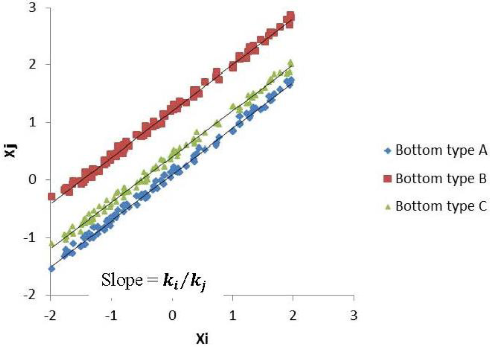
The bottom-type pixels are represented in a scatter plot of transformed radiance (X(λ)) bands i and j (Figure 1). If the relationship between radiance and depth is linear and the bottom type is constant, the plotted pixel will fall ideally on a straight line. The slope of this straight line represents the relative attenuation in each combination of bands. The different bottom types represented in a scatter plot should create a similar line, the variation along which indicates changes in depth. The gradient of each line would be identical because the ratio of the attenuation coefficients (ki/kj) is independent of bottom type. The y-intercept of each line is subsequently used, independent of depth, as an index of bottom type; this is known as the depth-invariance index (Yij), which can be written as:
The determination of the attenuation coefficient (quotient) can be achieved using a biplot (Figure 1) of the transformed radiance of the two bands (X(λ)i and X(λ)j). The biplot contains data for one uniform bottom type (i.e., sand) and variable depth. Thus, the depth-invariance index is scaled to the y-intercept. Based on this value on the y-axis, which represents the index of the bottom type, the pixels are then classified and the value of ki/kj is calculated for each combination of bands. The algorithm for calculating the attenuation coefficient only holds when pixels of the same object at different depths are distributed linearly for the paired bands [6]. It is created using the following equations [7]:
2.1. Lyzenga81 Correction Method
In Lyzenga’s 1981 correction method [7], sea-surface scattering (S(λ)) or atmospheric scattering (A(λ)) are implicitly assumed homogeneous over the target area. For deep water, the observed spectral radiance (L(λ)) at infinite h (L(λ)∞ ≡ limh→∞L(λ)) is assumed not to include bottom reflectance, such that the water depth only consists of information related to external reflection from the water surface and atmospheric scattering. Then, the effects of S(λ) or A(λ) can be removed by subtracting the average radiance of the deep water (L(λ)∞). The new equation for the transformed radiance is written as:
2.2. Lyzenga06 Correction Method
In Lyzenga’s 2006 correction method [12], sea-surface scattering (S(λ)) or atmospheric scattering (A(λ)) are not assumed homogeneous over the target area; they are expected to vary from pixel to pixel. Their variations are related linearly to the radiance of the NIR band, for which the exponential term of Equation (1) is negligible. The correction method removes the pixel-wise variations of S(λ) and A(λ) using the NIR band. Thus, we can expect a correlation between (L(λ)∞ and LNIR for an arbitrary visible wavelength. The new equation for the transformed radiance is written as:
3. Methodology
3.1. Study Area
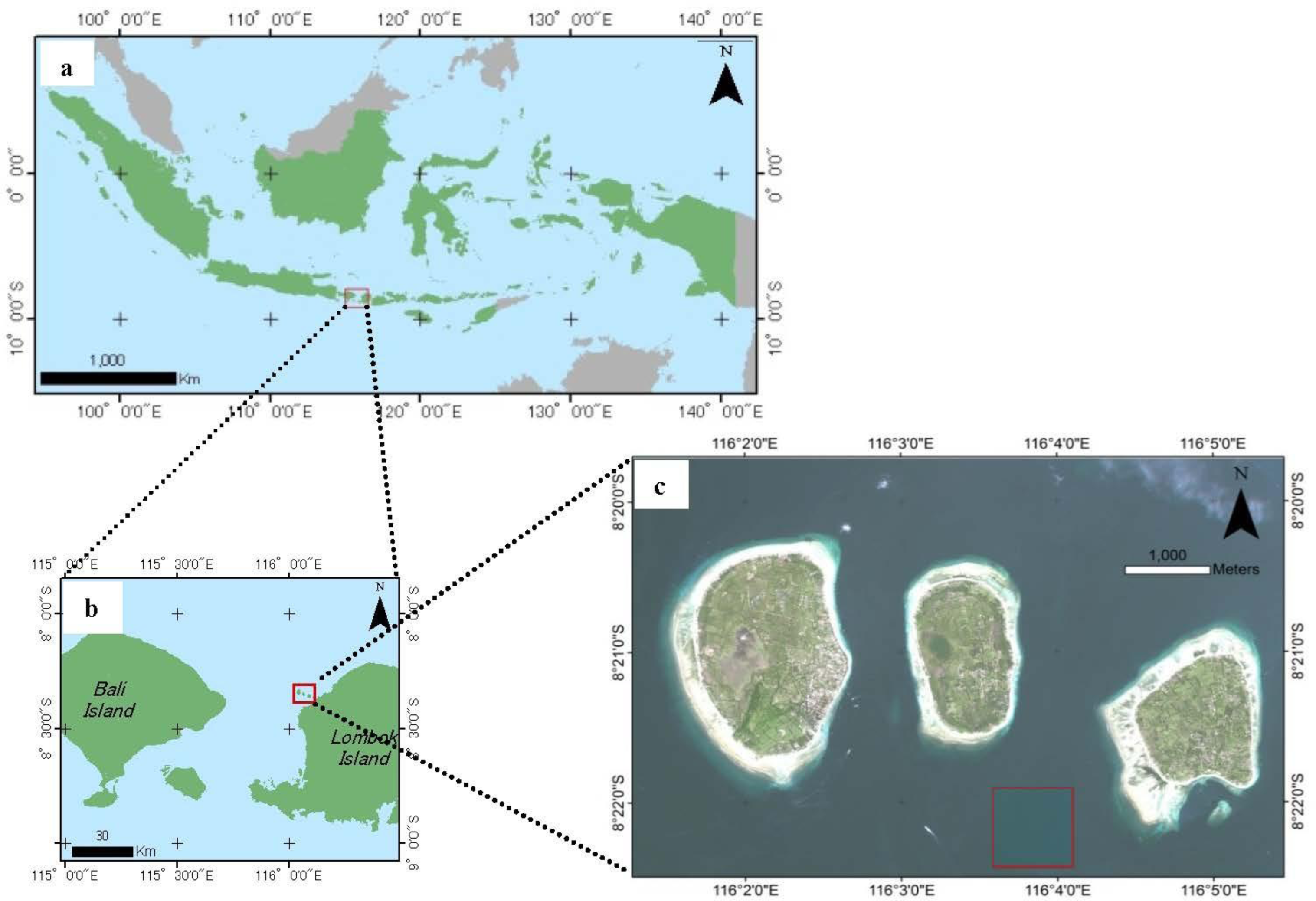
The study area, shown in Figure 2, is located in central southern Indonesia, off the coast of Lombok Island. Geographically, it spans 116°00′–116°08′E and 8°20′–8°23′S, encompassing an area to the northwest of Lombok Island. The Gili Matra Marine Natural Park includes three islands: Gili Trawangan, Gili Meno, and Gili Air. The Gili Matra Islands consist of a variety of shallow-water bottom types: hard coral, soft coral, dead coral, dead coral with algae, rubble, sand, and seagrass.
Several research projects have investigated the biodiversity of the Gili Matra Islands [21–23]. The reefs of the Gili Matra Islands contain several species of both hard and soft corals at depths in the range 1–30 m. Boulder brain coral, massive coral, branch coral, and foliose coral are species commonly found. The shallow-water area of Gili Meno contains highly productive areas of seagrass beds with Thallassia sp. the most abundant species. Seagrass beds provide a nursery habitat for several fish species, crab, and shrimp, in addition to providing feeding grounds for turtles. Gili Matra is famous for turtle migration routes as a feeding ground for turtle species.
3.2. Data Collection
3.2.1. Multispectral Imagery
The main characteristics of the imagery are summarized in the following list. The WorldView-2 imagery covers an area of 48 km2 of the Gili Matra Marine Natural Park. It is a Level 2A (L2A) data product supplied by the Hitachi Company, Japan. An L2A image has undergone radiometric and geometric corrections, and the WorldView-2 digital numbers are converted to physical units of Band-Averaged Spectral Radiance (W·m−2·sr−1·μm−1) [24].
WorldView-2 image specifications
Date: 25 January 2010
Time (GMT): 02:47:26.97 a.m.
Spatial resolution (m): 1.84 m at Nadir, 2.08 m at 20° off-nadir
Solar azimuth (deg): 116.3
Solar elevation (deg): 63.4
3.2.2. Ground Truth Data
The purpose of mapping focuses on major habitat types; thus, the survey methods should be simple, quick, and able to cover large areas. The manta tow technique is used to estimate general variations in the benthic communities of coral reefs, for which the unit of interest is either the entire reef or a large portion of it. Manta boards are large boards assembled from wood or glass-reinforced plastic that act as hydrofoils [4]. A modification of this technique is applied in this research by incorporating an underwater camera and the Global Positioning System (GPS) to record the bottom type along a transect, widely known as a belt transect. Technically, this requires two observers to swim along the belt transect and count the target benthic objects within the coral reef habitat. The length of each transect line is 20–100 m, and the underwater video technique records information within a belt 5 m wide. The data collection for the coral reef ecosystem of the Gili Islands is a collaborative effort between CReSOS (Center for Remote Sensing and Ocean Science, Udayana University—JAXA program) and the Research Institute for Marine Research and Observation (Ministry of Marine Affairs and Fisheries Republic of Indonesia). The observation data for the coral reef and seagrass were measured and analyzed by the Climate Change Research Team [23].
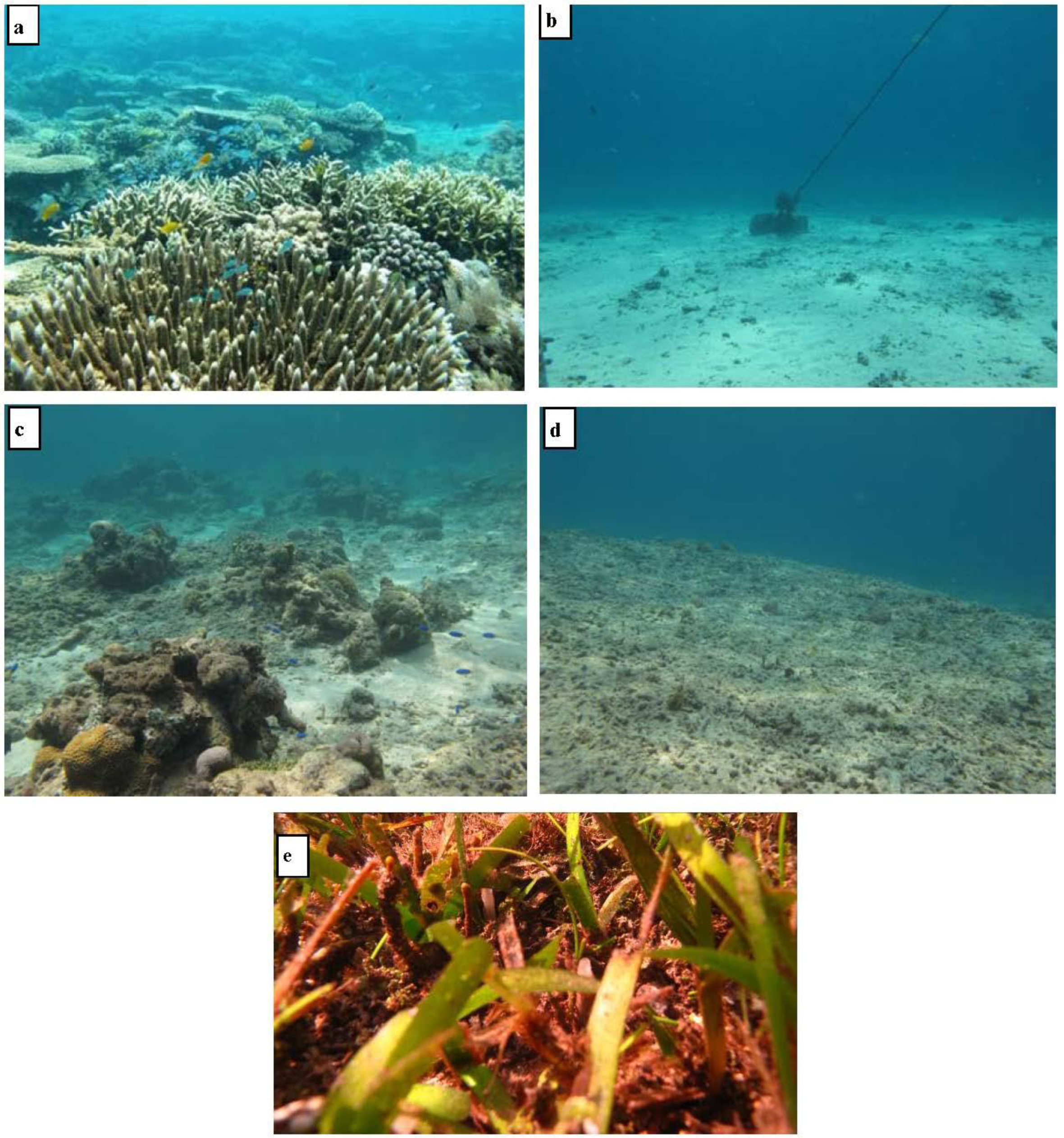
There are two types of data used in the analysis: transect belt video data analyzed at 10-m intervals, and rapid surveys. There are five different classes of bottom type identified from the video and visual observation, which is recognized as a coarse complexity class. Figure 3 presents photos of each bottom type taken in the Gili Mantra coral reef ecosystem, representing the major habitats.
The five bottom types identified are coral, sand, mixed bottom (i.e., sand, rock, coral, rubble, and seagrass), rubble, and seagrass. These bottom types are used as the habitat classes in the classification process. Based on the belt transect, rapid survey, and visual interpretation, 1100 points are identified for the 5 bottom types with 220 points for each type. In order to reduce the effect of spatial autocorrelation in the dataset, the training point was selected from Gili Air and Gili Meno sites, and Gili Trawangan became the control point.
3.3. Data Processing
3.3.1. Lyzenga’s Method
The preprocessing step in image processing is sensor calibration from digital numbers to the units of band-averaged spectral radiance. The equations and calibration coefficients applied are based on the Digital Globe technical note about radiometric use of WorldView-2 imagery [24]. The physical units of band-averaged spectral radiance are W·m−2·sr−1·μm−1. After the preprocessing step, the following steps are performed to apply Lyzenga’s method to WorldView-2 imagery.
The first step is selecting the deep-water area for the correction of atmospheric and sea-surface noise. There are three rules governing the selection of this area: it should not contain haze or cloud, sun glint or white caps. The averaged radiance values of the area of deep water (L(λ)∞ are used to calculate the depth-invariance index of the Lyzenga81 correction method. As shown in Equation (5)i band radiance values are subtracted by the averaged i band radiance values of the deep-water area. The deep-water area selected, based on visual inspection, is clear of noise from haze or cloud. Meanwhile, in the Lyzenga06 correction method, it is necessary to separate the α(λ)i0, α(λ)1NIR1, and α(λ)2NIR2 coefficients from the selected area of deep water. The coefficients are based on a linear function of the visible and NIR radiance. WorldView-2 imagery has two NIR bands that are beneficial for the correction based on Lyzenga06’s correction method; this research uses both NIR bands.
The second step is linearizing the relationship between radiance and depth to create the transformed radiance (X(λ)i). Based on Lyzenga’s method [6], the transformed radiance (X(λ)) is a linear value of radiance and depth. In the calculation of transformed radiance (X(λ)), the input is the noise-corrected radiance from Lyzenga’s correction methods (Lyzenga81 and Lyzenga06). The outcome of this step creates new bands as inputs for the next step.
In the third step, the known object pixels are applied to predict the ratio of the attenuation coefficients (ki/kj); sand is used because it is easily identified. The radiance value extracted from sand at various depths is used as input in Equations (3) and (4). Then, the attenuation coefficient is calculated for each band pair. The rule of band pairing is that a band only pairs once with another band. As shown in Table 1, three visible bands create three band pairs, while six visible bands create 15 band pairs. For each Lyzenga’s correction method, this research derived ratios of attenuation coefficients from the transformed radiance (X(λ)) values.
In the final step, the variable calculated above is added to the calculated depth-invariance index. A pair of bands is needed as an input with an attenuation coefficient for the same band pair. Each pair of spectral bands produces a single depth-invariant band. The data used in the classification process are the result of the depth-invariance index derived from Equation (2). The inputs for the classification process are the three and 15 depth-invariant bands from the three and six visible bands, respectively.
3.3.2. Supervised Classification
The maximum likelihood classifier is a supervised classification method, which attempts to envisage the output of the bottom-type class. The maximum-likelihood algorithm assumes normality within the training data, and the parametric rule should be approximated by having an appropriate sample size. If the statistical characterization is approximated, then the image classification approach uses the maximum-likelihood decision rule with equal probabilities of the classes [10]. The normal distribution of the statistics for each class in each band was a basic assumption in this classification method. The assumption is used to estimate the probability that a given pixel belongs to a particular class. The maximum likelihood method is applied to classify the bottom-type distribution using the depth-invariance indices, and the training area is used as the reference/training data. The following function is calculated for each pixel [25]:
i = class
x = n-dimensional data (where n is the number of bands)
p(ωi) = probability that class ωi occurs in the image; it is assumed to be the same for all classes
|∑i| = determinant of the covariance matrix of the data in class ωi
∑i−1 = its inverse matrix
mj= mean vector
3.3.3. Accuracy Test
The accuracy test was referenced to thematic accuracy, which has the non-positional characteristics of spatial data. If the data were to be subjected to hyperspectral or multispectral classification, then thematic accuracy would correlate to classification accuracy [26]. This accuracy refers to the correspondence between the class label and the “true” class, which is generally defined as that observed on the ground during field surveys [4]. In other words, it refers to how much of the class, which is labeled as coral reef on a classified image, is a coral reef in situ.
In this assessment, an error matrix (user accuracy) was used to identify object accuracy, and kappa analysis used to identify statistical difference accuracy. The accuracy of the predicted coral reef ecosystem map is represented as user accuracy. A user of this map will find that each time an area labeled as coral reef on the map is visited, there is only an n% probability that it is actually coral reef [4]. Moreover, the kappa statistic is an estimator of n parameters for a population of subjects and observers [27]. The kappa coefficient was first proposed by Cohen [28]. It measures whether two (or more) observers are independent by classifying items or observations into the same set of n mutually exclusive and exhaustive categories. It may be of interest to use a measure that summarizes the extent to which the observers agree in their classifications [29]. Based on kappa statistics, one can test whether two datasets have statistically different accuracies [30]. This statistical evaluation is used to assess the two Lyzenga correction methods in two cases.
3.3.4. Comparison Test
Four cases are evaluated in this research: the Lyzenga81 correction method with three visible bands, Lyzenga81 correction method with six visible bands, Lyzenga06 correction method with three visible bands, and Lyzenga06 correction method with six visible bands. In order to evaluate the improvement of spectral cover, the result of the accuracy test of higher spectral cover (six visible bands) is subtracted by the lower spectral cover (three visible bands) in both the Lyzenga81 and Lyzenga06 corrections. Similarly, the result of the accuracy test of the Lyzenga06 correction is subtracted by the Lyzenga81 correction in both cases of three and six visible bands to evaluate the improvement of Lyzenga’s methods.
4. Results and Discussion
4.1. Performance of Image Correction
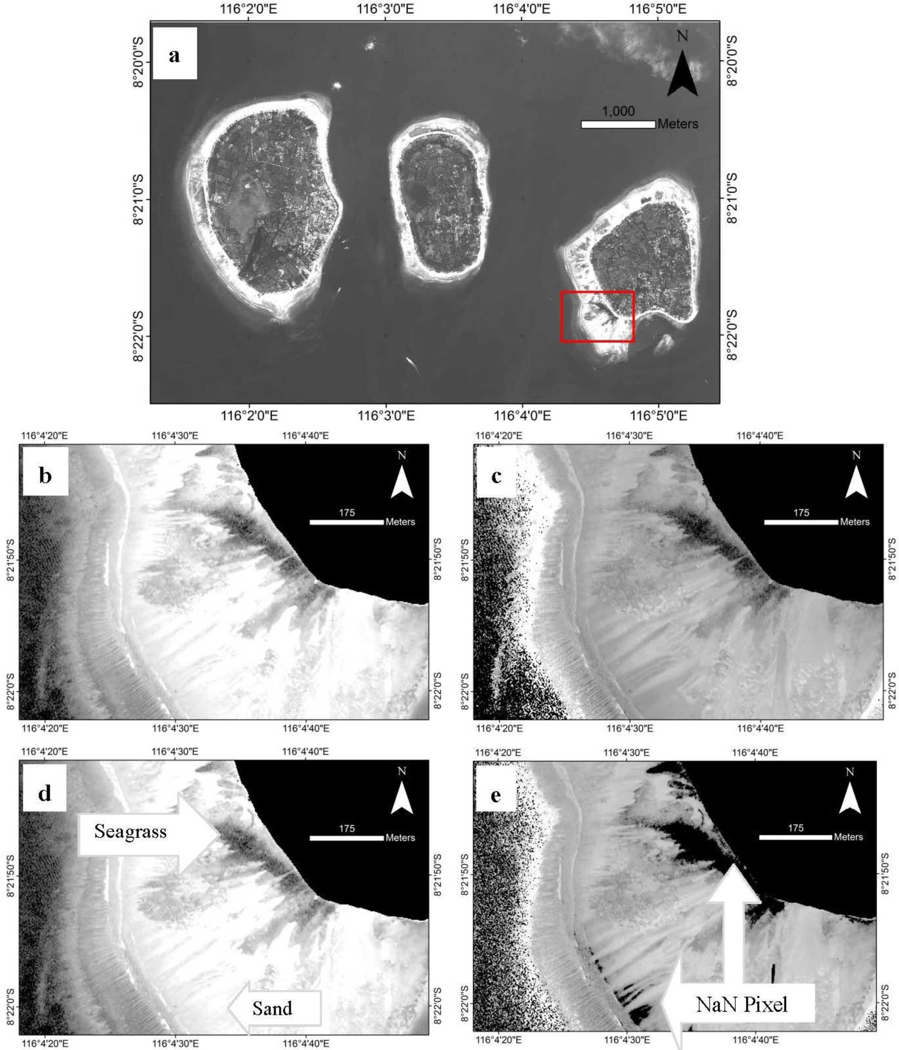
The Gili Matra Islands’ shallow-water ecosystems have bottom types at various depths; hence, the Lyzenga method is suitable for application [7]. Satellite imagery of the Gili Matra coral reef ecosystem contains noise from the atmosphere and water body and thus the light-scattering and absorption noise must be corrected by applying Lyzenga’s correction methods. The results of both Lyzenga correction methods in the transformed radiance values are shown in Figure 4. The algorithms produce considerable correction of the noise based on the resulting images.
Figure 4 shows that the Lyzenga06 correction method transformation generates a non-value (NaN) pixel for two object types, which are dense seagrass and bright sand (marked in Figure 4e). Sand radiance in very shallow water does not follow the assumption that radiance in the NIR band is absorbed completely by the water. Radiance emitted from the sand in any NIR band is higher than the absorption properties of the water. Meanwhile, the dense seagrass radiance is similar or slightly lower in value to the radiance of the deep-water area, especially for low wavelengths, i.e., coastal and blue band. The radiance has low value and appears dark (Figure 4b,d) because the areas of seagrass absorbed the light. Based on Equation (6) of the Lyzenga06 correction method, the calculated visible bands, which are subtracted from the NIR band after multiplication with the α(λ) coefficient, produce a negative value of the log function in this case. In order to describe the NaN pixel that appears in the Lyzenga06 correction method, we perform a simple algebraic description, as below:
In other cases of coral reef ecosystems with different bottom-type characteristics, the reflectance of the bottom object is low in the NIR band. High reflectance of bottom type in shallow water is not only due to the high reflectance of the bottom, but also the adjacent effect. It is referred to as the effect of high reflectance emitted from objects in the coastal area, which are very close to the water body and being scattered in the atmosphere above the water area. The information recorded by the satellite not only consists of information of the water and spectral object below the surface, but also of the spectral object near the water body.
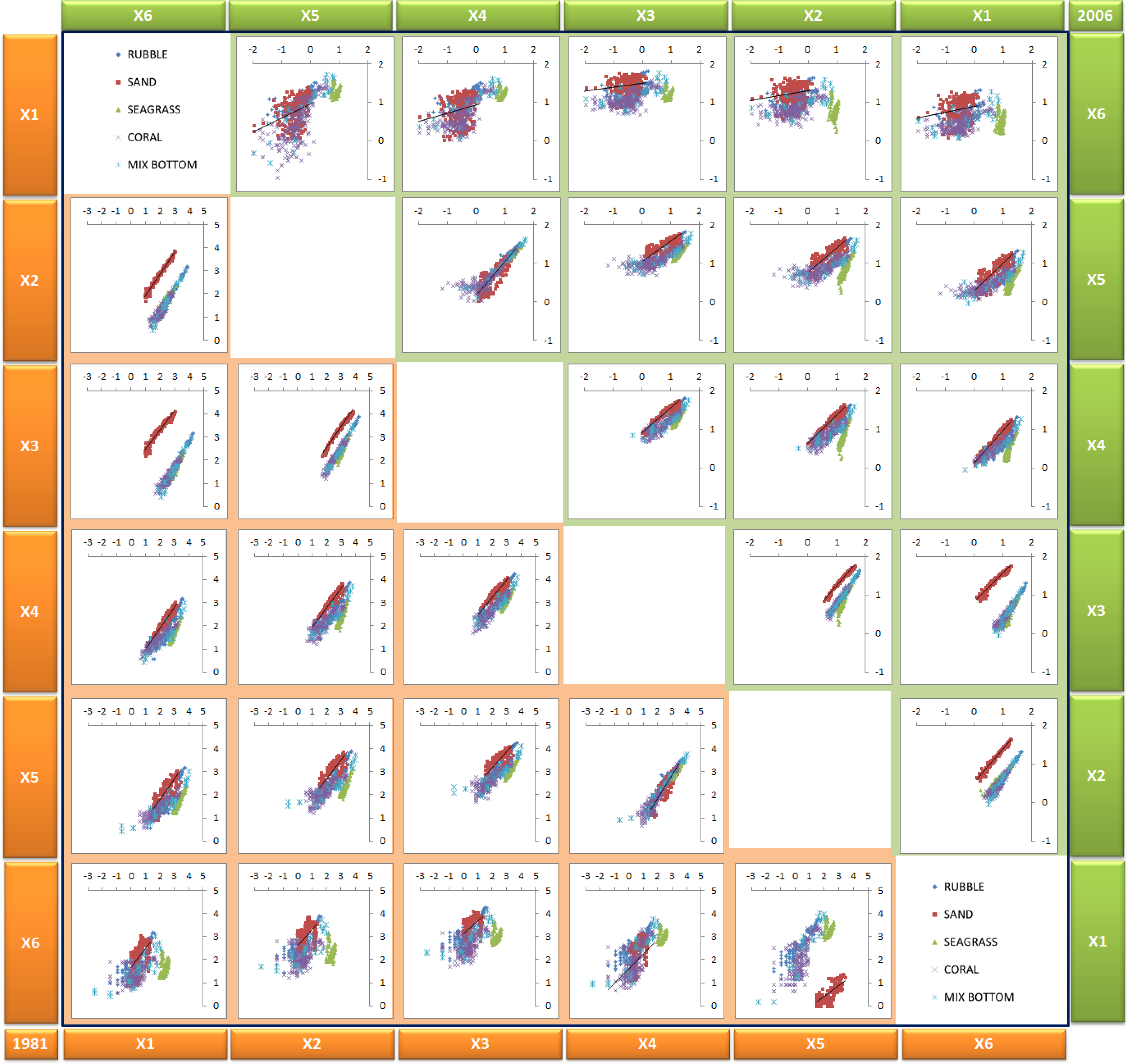
Another research [16,20] has concluded that the application of two other NIR bands (NIR1 and NIR2) to WorldView-2 imagery is useful for the removal of sun glint (atmospheric noise). Furthermore, this study has discovered an additional advantage of utilizing two NIR bands of WorldView-2 imagery, which is the automatic masking of the land, shallow-water, and deep-water areas. The delineation between deep and shallow water can be correctly applied in pixels with low noise. However, for the case of the Gili Islands’ shallow-water coral reef ecosystems, some objects’ reflectance appear in the shallow-water area in the NIR band. This implies that the correction theory is not complete in the assumption that the NIR band does not include volume scattering or bottom-type reflectance. In reality, the sand object in the shallow water of the research area is very bright and exhibits a reflectance signal, even in the NIR band. In other words, the reflectance of the sand object is still greater than the water. This study also noticed that the NIR1 band (770–895 nm) is close to the visible domain and is still sensitive to bottom reflectance. The transformed radiance (X(λ)) for the Lyzenga81 and Lyzenga06 correction methods assumes that atmospheric and sea-surface scattering noise has been corrected. The results of the transformed radiance for each known bottom type are plotted in Figure 5 as a 2-D scatter plot. The scatter plot shows that the known object pixels do not fall on a perfect line. Moreover, the number of scattered pixels gradually increases with higher wavelengths (from X1 to X6). According to Lyzenga’s theory [7], different bottom types should lie on a straight line and parallel one another, as shown in Figure 1. The scattered distribution mentioned here probably occur because of two points. First, the atmospheric and sea-surface scattering noise has not been corrected perfectly. Second, the higher wavelengths contain higher noise because of the sensitivity to the water column. However, higher wavelength bands still usefully distinguish bottom type classes, specifically in combination with all bands.
4.2. Image Classification Analysis
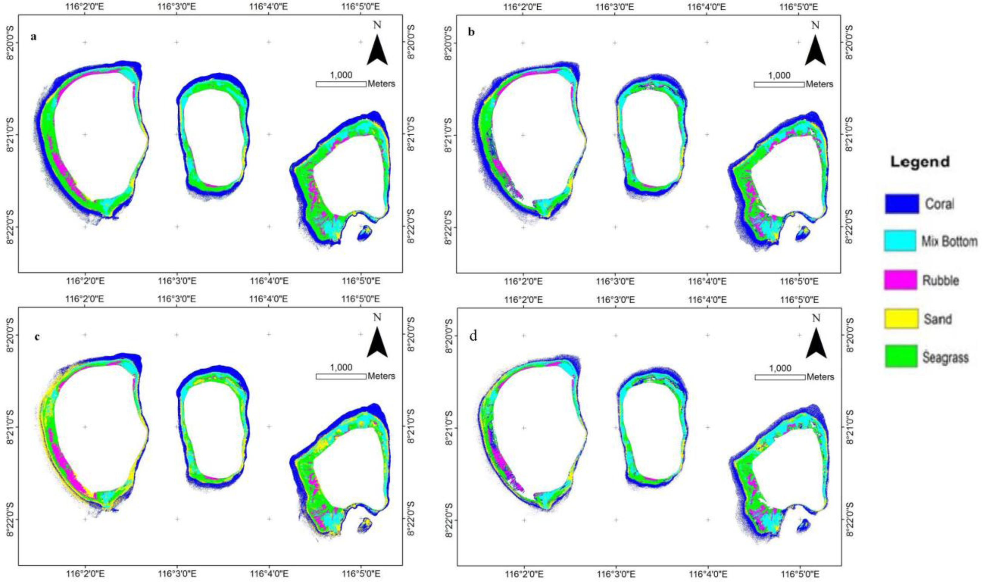
In the research area, sand, rubble, seagrass, and live coral reefs were the most abundant bottom types in the shallow coral reef ecosystem. Although these features have different spectral characteristics and they can be separated as homogeneous pixels, in reality, there can be significant intermixing between them, even with spatial resolution of 2 × 2 m. Furthermore, complex feature combinations, categorized as mixed bottom type, define inseparable objects in the field observations. A training point for five bottom types was created as a reference for the maximum likelihood classification. Based on combinations of the depth-invariance bands from the Lyzenga81 and Lyzenga06 correction methods, using different numbers of visible bands, the classification results were obtained (Figure 6).
Visual interpretation of Figure 6a,b, based on the combined depth-invariance indices of the three visible bands, shows a complex distribution, but most of which is misclassified. Both methods for this number of visible bands show the misclassification of rubble and seagrass. The combined depth-invariance indices of the three visible bands are unable to separate this information because seagrass and rubble are always presented with different percentage cover in each pixel. Figure 6c,d shows that the combination of depth-invariance indices for the six visible bands for each method could differentiate the coarse bottom-type classification. The mixed bottom type is frequently misclassified as seagrass; however, in the Lyzenga06 correction, the number of misclassifications is reduced.
The techniques of accuracy assessment are based on statistical calculations derived from the confusion matrix, which compares the output of classified and control pixel data. Classification accuracies for each method, obtained with WorldView-2 imagery, are provided in Table 2, together with the overall accuracy and kappa coefficient. Individual bottom types exhibit different classification accuracies. Values of class definition similarity, at the coarse descriptive level, vary from 58% to 98%. These numbers represent the degree of uniformity among the factors defining each bottom type class. For instance, rubble is always very well classified (e.g., 93% to 98% user accuracy). Conversely, mixed bottom is poorly classified with the combined depth-invariance indices of the three visible bands (i.e., 66% to 69%), but the accuracy is higher for the six visible bands (i.e., 74% to 80%). The trigger could be because of the heterogeneity of bottom objects and because the low spectral data of mixed objects does not allow the objects to be separated accurately. The accuracy of identification of sand and seagrass is high (i.e., 72% to 97%) for both methods and combined depth-invariance indices. Coral identification exhibits wide variation in accuracy (i.e., 58% to 86%). The highest overall accuracy of WorldView-2 imagery analysis is achieved using the Lyzenga81 correction method with the combined depth-invariance indices of the six visible bands. This achieved an overall accuracy of 90% and it remained significantly high throughout the analysis (>80%) for each bottom type. The value of the overall kappa statistic exhibits a moderate value (0.71 and 0.73) for the application of three visible bands and it is high for the application of six visible bands (0.81 and 0.86). This statistic estimates the percentage of successful classifications compared with a random chance classification assignment.
Based on the classification results for all the cases, the rubble is located relatively close to the shoreline, as is seagrass that is mixed with rubble and sand in numerous parts of the island. On the other hand, corals were identified along the edge of the shallow area bordering the deeper water (escarpment area).
Table 3 shows that the most influential factor for improving the accuracy in this case is spectral resolution rather than the method of image noise correction. The improvement of spectral resolution from three to six bands could enhance the overall accuracy by 28% and 16% for the Lyzenga81 and Lyzenga06 correction methods, respectively. On the other hand, it is not clear which noise correction method gives better overall accuracy; the Lyzenga06 correction method is slightly (2%) better for the case with three bands and the Lyzenga06 correction method is slightly (4%) better for the six band case. However, the noise correction method significantly affects the classification accuracy for some bottom types. For example, the accuracy for coral in the three-band case changes by 10% depending on the choice of the noise correction method. For the three visible bands, many misclassifications occur for both methods and each object except rubble.
Theoretically, the Lyzenga06 correction method is able to increase the accuracy of bottom-type identification. However, the enhanced method could only improve the low spectral resolution, whereas for the high spectral resolution, this method reduces the accuracy. Additionally, the result shows that the basic Lyzenga81 correction algorithm is the best method for identifying bottom type using the applied combined depth-invariance indices of the six visible bands in the Gili Islands’ shallow-water coral reef ecosystem. The trigger could be because the NIR band applied in the Lyzenga06 correction is sensitive to bottom spectral reflectance and the adjacent effect; thus, the theory does not hold for correcting sea-surface scattering and atmospheric noise. In summary, spectral resolution is more important than noise correction for improving the accuracy of bottom-type identification.
The classification level applied in this research is a coarse description of the bottom type (e.g., coral, seagrass, rubble, sand, and mixed bottom). It is possible to implement an intermediate–fine description classification level using high-resolution WorldView-2 imagery, if supported with appropriate field data. Applying the method for a large number of bottom materials poses some problems because of the similarity in the reflectance of several materials, such as vegetation and mud [6].
5. Conclusions
In this study, Lyzenga’s bottom-type identification method was applied to WorldView-2 imagery for the first time. For the correction of the atmospheric and sea-surface scattering, two different approaches proposed by Lyzenga (Lyzenga06 and Lyzenga81) were applied. In addition, two different combinations of visible bands were used: all six of the visible bands of WorldView-2 and the three bands corresponding to common high-resolution multispectral sensors.
The Lyzenga06 correction method, which utilizes the near infrared (NIR) bands, was more accurate than the Lyzenga81 correction method only for the case of three visible bands. This result indicates that the superiority of the Lyzenga06 correction method is case-dependent. Moreover, the Lyzenga06 correction method could not be applied for two bottom types in very shallow water, i.e., dense seagrass and bright sand.
The used of six visible bands in the identification accuracy was better than only three bands, regardless of the correction method. This result shows that a large number of visible bands of multispectral data, used for water-column correction, improve the accuracy of bottom-type identification in shallow-water coral reefs. Furthermore, this research only evaluated one scene of WorldView-2 imagery. Correspondingly, it is necessary to evaluate several sites with different characteristics to analyze the variability of shallow-water coral reef ecosystems. Therefore, future work should examine multi-site coral reef ecosystems; however, it is expected that the findings will probably be site-dependent.
Acknowledgments
This research was funded by the Indonesia Ministry of Finance, through the Indonesia Endowment Fund Scholarship, and the Indonesia Institute of Marine Research and Observation. The authors would like to thank the Hitachi Company, Japan, for providing the WorldView-2 Image data. We are very grateful to Tatsuku Tanaka and Takahiro Osawa of CReSOS, Bali, for scientific advice on evaluating coral reef ecosystems. Thanks go also to Suciadi, Camelia Kusuma, Iis Triyulianti, and Nyoman Surana for their assistance in the field.
Author Contributions
Masita Dwi Mandini Manessa processed all the data, interpreted the results, and wrote the manuscript. Ariyo Kanno supervised the research and also helped manuscript writing. Masahiko Sekine gave a number of suggestions that significantly improved the paper. Masita Dwi Mandini Manessa, E. Elvan Ampou, and Nuryani Widagti contributed to the collection and analysis of ground reference data. Abd. Rahman As-syakur assisted with refining manuscript revision.
Conflicts of Interest
The authors declare no conflict of interest.
References
- Benfield, S.L.; Guzman, H.M.; Mair, J.M.; Young, J.A.T. Mapping the distribution of coral reefs and associated sublittoral habitats in Pacific Panama: A comparison of optical satellite sensors and classification methodologies. Int. J. Remote Sens 2007, 28, 5047–5070. [Google Scholar]
- Wongprayoon, S.; Vieira, C.A.O.; Leach, J.H.J. Spatial Accuracy Assessment for Coral Reef Classification. In proceeding of the XIII Brazilian Remote Sensing Symposium, Florianopolis, Brazil, 21–26 April 2007; pp. 6273–6281.
- Helmy, A.K.; El-Taweel, G.S. Neural network change detection model for satellite images using textural and spectral characteristics. Am. J. Eng. Appl. Sci 2010, 3, 604–610. [Google Scholar]
- Green, E.P.; Mumby, P.J.; Clark, C.D.; Edwards, T.M. Remote Sensing Handbook for Tropical Coastal Management; Coastal Management Sourcebooks, 3; UNESCO Publishing: Paris, France, 2000. [Google Scholar]
- Nurlidiasari, M.; Budiman, S. Mapping coral reef habitat with and without water column correction using Quickbird image. Int. J. Remote Sens. Earth Sci 2005, 2, 45–56. [Google Scholar]
- Lyzenga, D.R. Passive remote sensing techniques for mapping water depth and bottom features. Appl. Opt 1978, 17, 379–383. [Google Scholar]
- Lyzenga, D.R. Remote sensing of bottom reflectance and water attenuation parameters in shallow water using Aircraft and Landsat data. Int. J. Remote Sens 1981, 2, 72–82. [Google Scholar]
- Pahlevan, N.; Valadanzouj, M.; Alimohamadi, A. A. Quantitative Comparison to Water Column Correction Techniques for Benthic Mapping Using High Spatial Resolution Data. Proceedings of the ISPRS Commission VII Mid-term Symposium “Remote Sensing, from Pixels to Processes”, Enschede, The Netherlands, 8–11 May 2006; pp. 286–291.
- Vinluan, R.J.N.; Alban, J.D.T.D. Evaluation of Landsat 7 ETM+ Data for Coastal Habitat Assessment in Support of Fisheries Management. Proceedings of the 22nd Asian Conference on Remote Sensing, Singapore, 5–9 November 2001; pp. 1356–1361.
- Vanderstraete, T.; Goossens, R.; Ghabour, T.K. Coral reef habitat mapping in the red sea (Hurghada, Egypt) based on remote sensing. EARSeL eProc 2004, 3, 191–206. [Google Scholar]
- Andrefouet, S.; Kramer, P.; Pulliza, D.T.; Joyce, K.E.; Hochberg, E.J.; Perez, R.G.; Mumby, P.J.; Riegl, B.; Yamano, H.; White, W.H. Multi-site evaluation of IKONOS data for classification of tropical coral reef environments. Remote Sens. Environ 2003, 88, 128–143. [Google Scholar]
- Lyzenga, D.R.; Malinas, N.P.; Tanis, F.J. Multispectral bathymetry using a simple physically based algorithm. IEEE Trans. Geosci. Remote Sens 2006, 44, 2251–2259. [Google Scholar]
- Kanno, A.; Tanaka, Y. Modified Lyzenga’s method for estimating generalizes coefficients of satellite-based prediction of shallow water depth. IEEE Geosci. Remote Sens. Lett 2011, 9, 715–719. [Google Scholar]
- Kanno, A.; Tanaka, Y.; Kurosawa, A.; Sekine, M. Generalized Lyzenga’s predictor of shallow water depth for multispectral satellite imagery. Marine Geod 2013, 36, 1–12. [Google Scholar]
- Chen, P.; Liew, S.C.; Lim, R.; Kwoh, L.K. Mapping Coastal Ecosystems of an Offshore Landfill Island Using Worldview-2 High Resolution Satellite Imagery. Proceedings of the 34th International Symposium on Remote Sensing of Environment, Sydney, Australia, 10–15 April 2011; pp. 10–15.
- Paringit, E.C. Shallow Water Bathymetry Mapping and Benthic Cover Estimation using Worldview-2 High Spatial Resolution Imagery. Proceedings of the 32nd Asian Conference on Remote Sensing (ACRS), Taipe, Taiwan, 3–7 October 2011; pp. 652–655.
- Collin, A.; Planes, S. Enhancing coral health detection using spectral diversity indices from worldview-2 imagery and machine learners. Remote Sens 2012, 4, 3244–3264. [Google Scholar]
- Vahtmäe, E.; Kutser, T. Classifying the baltic sea shallow water habitats using image-based and spectral library methods. Remote Sens 2013, 5, 2451–2474. [Google Scholar]
- Lee, K.R.; Kim, A.M.; Olsen, R.C.; Kruse, F.A. Using WorldView-2 to determine bottom-type and bathymetry. Proc. SPIE 2011, 8030. [Google Scholar] [CrossRef]
- Collin, A.; Archambault, P.; Planes, S. Bridging ridge-to-reef patches: Seamless classification of the coast using very high resolution satellite. Remote Sens 2013, 5, 3583–3610. [Google Scholar]
- Djohar, I. Kondisi Karang Scleractinia Pada Daerah Rataan Dan Lereng Terumbu Karang di Taman Wisata Alam Laut GIli Indah, Lombok, NTB. Undergraduate Thesis, Bogor Agricultural University, Bogor, Indonesia, 1999 (in Indonesian). Available online: http://repository.ipb.ac.id/handle/123456789/23816 (accessed on 20 May 2011).
- Muhlis, M. Ekosistem terumbu karang dan kondisi oseanografi perairan kawasan wisata bahari Lombok. Berk. Penel. Hayati 2009, 26, 111–118. (in Indonesian). Available online: http://www.berkalahayati.org/index.php/bph/article/view/592 (accessed on 23 May 2011). [Google Scholar]
- Climate Change Research Team, Observation and Study on Marine Protected Area, Research Report; Research Institute for Marine Observation, Ministry of Marine Affairs and Fisheries: Negara, Bali, Indonesia, 2011.
- Digital Globe. Radiometric Use of WorldView-2 Imagery. Available online: http://www.digitalglobe.com/downloads/Radiometric_Use_of_WorldView-2_Imagery.pdf (accessed on 10 June 2012).
- Research System Inc, ENVI Online Help; Research System Inc.: Boulder, CO, USA, 2009.
- Stehman, S.V. Selecting and interpreting measures of thematic classification accuracy. Remote Sens. Environ 1997, 62, 77–89. [Google Scholar]
- Abraira, V.; Vargas, A.P.D.; Cajal, H.R. Generalization of the kappa coefficient for ordinal categorical data, multiple observers and incomplete designs. Questiio 1999, 23, 561–571. [Google Scholar]
- Cohen, J. A coefficient of agreement for nominal scales. Educ. Psychol. Meas 1960, 20, 37–46. [Google Scholar]
- Kvalseth, T.O. Kappa Coefficient of Agreement. In International Encyclopedia of Statistical Science; Lovric, M., Ed.; Springer: Berlin, Germany, 2011; pp. 710–713. [Google Scholar]
- Smith, R.B. Remote Sensing of Environment; MicroImages Inc.: Lincoln, NE, USA, 2012. [Google Scholar]


| a. Three Visible Bands Pair | b. Six Visible Bands Pair | |||||
|---|---|---|---|---|---|---|
| 1. coastal vs. blue | 2. coastal vs. green | 3. coastal vs. yellow | 4. coastal vs. red | 5. coastal vs. red edge | ||
| 1. blue vs. green | 2. blue vs. red | 6. blue vs. green | 7. blue vs. yellow | 8. blue vs. red | 9. blue vs. red edge | |
| 3. green vs. red | 10. green vs. yellow | 11. green vs. red | 12. green vs. red edge | |||
| 13. yellow vs. red | 14. yellow vs. red edge | |||||
| 15. red vs. red edge | ||||||
| Lyzenga06 with 3 Visible Bands | Lyzenga81 with 3 Visible Bands | Lyzenga06 with 6 Visible Bands | Lyzenga81 with 6 Visible Bands | |
|---|---|---|---|---|
| Coral | 78.08% | 58.46% | 88.56% | 89.22% |
| Mix Bottom | 60.49% | 62.57% | 76.45% | 87.61% |
| Rubble | 99.80% | 100.00% | 100.00% | 100.00% |
| Sand | 90.18% | 80.35% | 94.02% | 94.46% |
| Seagrass | 83.04% | 90.42% | 90.97% | 93.40% |
| Overall Accuracy | 80.73% | 78.29% | 89.31% | 92.86% |
| Kappa | 0.76 | 0.73 | 0.87 | 0.91 |
| Improvement by Lyzenga’s Method in 3 Visible Bands | Improvement by Lyzenga’s Method in 6 Visible Bands | Improvement by Spectral Coverage in Lyzenga81 | Improvement by Spectral Coverage in Lyzenga06 | |
|---|---|---|---|---|
| Coral | 19.62% | −0.66% | 30.76% | 10.48% |
| Mix Bottom | −2.08% | −11.16% | 25.03% | 15.96% |
| Rubble | −0.20% | 0.00% | 0.00% | 0.20% |
| Sand | 9.83% | −0.43% | 14.10% | 3.84% |
| Seagrass | −7.38% | −2.44% | 2.98% | 7.92% |
| Overall Accuracy | 2.45% | −3.55% | 14.57% | 8.57% |
| Kappa | 0.03 | −0.04 | 0.18 | 0.10 |
© 2014 by the authors; licensee MDPI, Basel, Switzerland This article is an open access article distributed under the terms and conditions of the Creative Commons Attribution license (http://creativecommons.org/licenses/by/3.0/).
Share and Cite
Manessa, M.D.M.; Kanno, A.; Sekine, M.; Ampou, E.E.; Widagti, N.; As-syakur, A.R. Shallow-Water Benthic Identification Using Multispectral Satellite Imagery: Investigation on the Effects of Improving Noise Correction Method and Spectral Cover. Remote Sens. 2014, 6, 4454-4472. https://0-doi-org.brum.beds.ac.uk/10.3390/rs6054454
Manessa MDM, Kanno A, Sekine M, Ampou EE, Widagti N, As-syakur AR. Shallow-Water Benthic Identification Using Multispectral Satellite Imagery: Investigation on the Effects of Improving Noise Correction Method and Spectral Cover. Remote Sensing. 2014; 6(5):4454-4472. https://0-doi-org.brum.beds.ac.uk/10.3390/rs6054454
Chicago/Turabian StyleManessa, Masita Dwi Mandini, Ariyo Kanno, Masahiko Sekine, Eghbert Elvan Ampou, Nuryani Widagti, and Abd. Rahman As-syakur. 2014. "Shallow-Water Benthic Identification Using Multispectral Satellite Imagery: Investigation on the Effects of Improving Noise Correction Method and Spectral Cover" Remote Sensing 6, no. 5: 4454-4472. https://0-doi-org.brum.beds.ac.uk/10.3390/rs6054454