
Remote Sensing of Sonoran Desert Vegetation Structure and Phenology with Ground-Based LiDAR

 ,
,
Abstract
:1. Introduction

| Year | 1906 | 1968 | 1978 | 1985 | 2001 | 2010 | 2012 |
|---|---|---|---|---|---|---|---|
| Species | Cover (%) | ||||||
| Acacia constricta | Nm * | 1.26 | 1.17 | 1.59 | 1.30 | 1.43 | 1.63 |
| Acacia greggii | Nm | 0.00 | 0.57 | 0.78 | 0.00 | 0.00 | 0.00 |
| Ambrosia deltoidea | Nm | 29.47 | 23.43 | 35.08 | 24.99 | 8.49 | 11.85 |
| Carnegiea gigantean | Nm | 0.08 | 0.04 | 0.07 | 0.19 | 0.13 | 0.16 |
| Cylindropuntia fulgida | Nm | 0.00 | 0.00 | 0.00 | 0.59 | 1.17 | 0.94 |
| Cylindropuntia leptocaulis | Nm | 0.54 | 0.74 | 1.12 | 0.00 | 0.17 | 0.25 |
| Cylindropuntia versicolor | Nm | 0.00 | 0.09 | 0.22 | 0.70 | 1.61 | 1.85 |
| Dyssodia pentachaeta | Nm | 0.19 | 0.00 | 0.00 | 0.00 | 0.00 | 0.00 |
| Echinocereus fasciculatus | Nm | 0.00 | 0.00 | 0.02 | 0.00 | 0.02 | 0.03 |
| Ferocactus wizlizenii | Nm | 0.00 | 0.00 | 0.00 | 0.00 | 0.02 | 0.03 |
| Isocoma tenuisectus | Nm | 0.00 | 0.00 | 0.01 | 0.00 | 0.00 | 0.00 |
| Krameria grayi | Nm | 0.00 | 0.00 | 0.00 | 0.14 | 0.06 | 0.06 |
| Larrea tridentata | Nm | 3.62 | 2.46 | 4.17 | 8.09 | 8.81 | 9.07 |
| Mammillaria grahamii | Nm | 0.00 | 0.00 | 0.01 | 0.00 | 0.00 | 0.00 |
| Muhlenbergia porter | Nm | 0.16 | 0.03 | 0.00 | 0.00 | 0.00 | 0.00 |
| Opuntia engelmannii | Nm | 0.00 | 1.50 | 3.53 | 0.55 | 2.30 | 2.83 |
| Psilostrophe cooperi | Nm | 1.17 | 0.01 | 0.00 | 0.00 | 0.00 | 0.00 |
| Tiqulia canescens | Nm | 0.00 | 0.00 | 0.00 | 0.00 | 0.00 | 0.00 |
| Unknown | Nm | 0.00 | 0.03 | 0.00 | 0.00 | 0.00 | 0.00 |
| Zinna pumila | Nm | 0.09 | 0.00 | 0.00 | 0.00 | 0.00 | 0.00 |
| Totals | 36.58 | 30.07 | 46.60 | 36.55 | 24.21 | 28.70 | |
Objectives
| Year | 1906 | 1968 | 1978 | 1985 | 2001 | 2010 | 2012 |
|---|---|---|---|---|---|---|---|
| Species | Density (Individuals/ha) | ||||||
| Acacia constricta | 609 | 406 | 406 | 406 | 203 | 101 | 101 |
| Acacia greggii | 0 | 0 | 101 | 101 | 0 | 0 | 0 |
| Ambrosia deltoidea | 0 | 25,761 | 24,848 | 24,341 | 20,588 | 12,475 | 12,373 |
| Carnegiea gigantean | 101 | 101 | 101 | 101 | 203 | 203 | 203 |
| Cylindropuntia fulgida | 203 | 0 | 0 | 0 | 101 | 0 | 101 |
| Cylindropuntia leptocaulis | 0 | 203 | 609 | 811 | 406 | 0 | 203 |
| Cylindropuntia versicolor | 0 | 0 | 101 | 101 | 203 | 304 | 203 |
| Dyssodia pentachaeta | 0 | 3043 | 0 | 0 | 0 | 0 | 0 |
| Echinocereus fasciculatus | 406 | 0 | 101 | 609 | 0 | 101 | 101 |
| Ferocactus wizlizenii | 0 | 0 | 0 | 0 | 0 | 101 | 101 |
| Isocoma tenuisectus | 203 | 0 | 0 | 203 | 0 | 0 | 0 |
| Krameria grayi | 0 | 0 | 0 | 0 | 203 | 406 | 406 |
| Larrea tridentata | 101 | 203 | 710 | 507 | 913 | 1116 | 1116 |
| Mammillaria grahamii | 0 | 0 | 101 | 101 | 1217 | 101 | 203 |
| Muhlenbergia porter | 0 | 101 | 203 | 0 | 0 | 0 | 0 |
| Opuntia engelmannii | 0 | 101 | 406 | 406 | 406 | 304 | 304 |
| Psilostrophe cooperi | 3144 | 5274 | 101 | 0 | 0 | 0 | 0 |
| Tiqulia canescens | 0 | 0 | 0 | 0 | 0 | 101 | 0 |
| Unknown | 101 | 0 | 101 | 0 | 0 | 0 | 0 |
| Zinna pumila | 0 | 406 | 0 | 0 | 0 | 0 | 0 |
| Totals | 4868 | 35,598 | 27,890 | 27,687 | 24,442 | 15,314 | 15,415 |
2. Methods
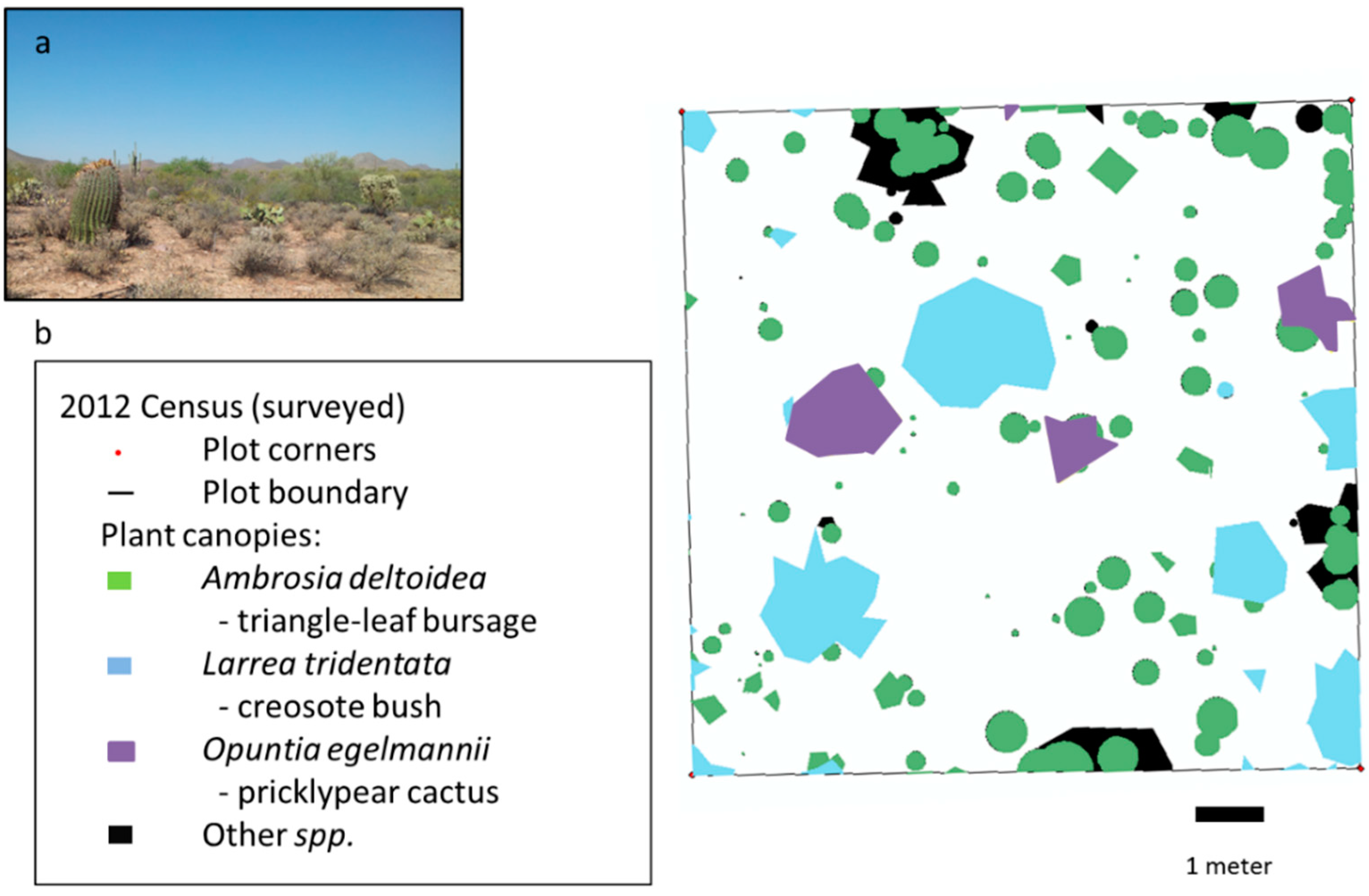
2.1. Study Site

| Species | N | Canopy Height (m) | Canopy Area (m2) | ||
|---|---|---|---|---|---|
| Mean | SE | Mean | SE | ||
| Ambrosia deltoidea | 25 | 0.40 | 0.02 | 0.14 | 0.02 |
| Larrea tridentata | 15 | 1.07 | 0.12 | 0.8 | 0.23 |
| Opuntia engelmannii | 4 | 0.61 | 0.06 | 0.74 | 0.29 |
| Cylindropuntia leptocaulis | 2 | 0.78 | 0.26 | 0.24 | 0.16 |
| Cylindropuntia versicolor | 2 | 1.8 | -- * | 1.48 | 0.79 |
| Acacia constricta | 1 | 1.70 | -- | 2.07 | -- |
| Krameria grayi | 1 | 0.20 | -- | 0.04 | -- |
| Cylindropuntia fulgida | 1 | 2.35 | -- | 1.47 | -- |
| Total | 51 | 0.70 | 0.07 | 0.50 | 0.10 |
2.2. Census
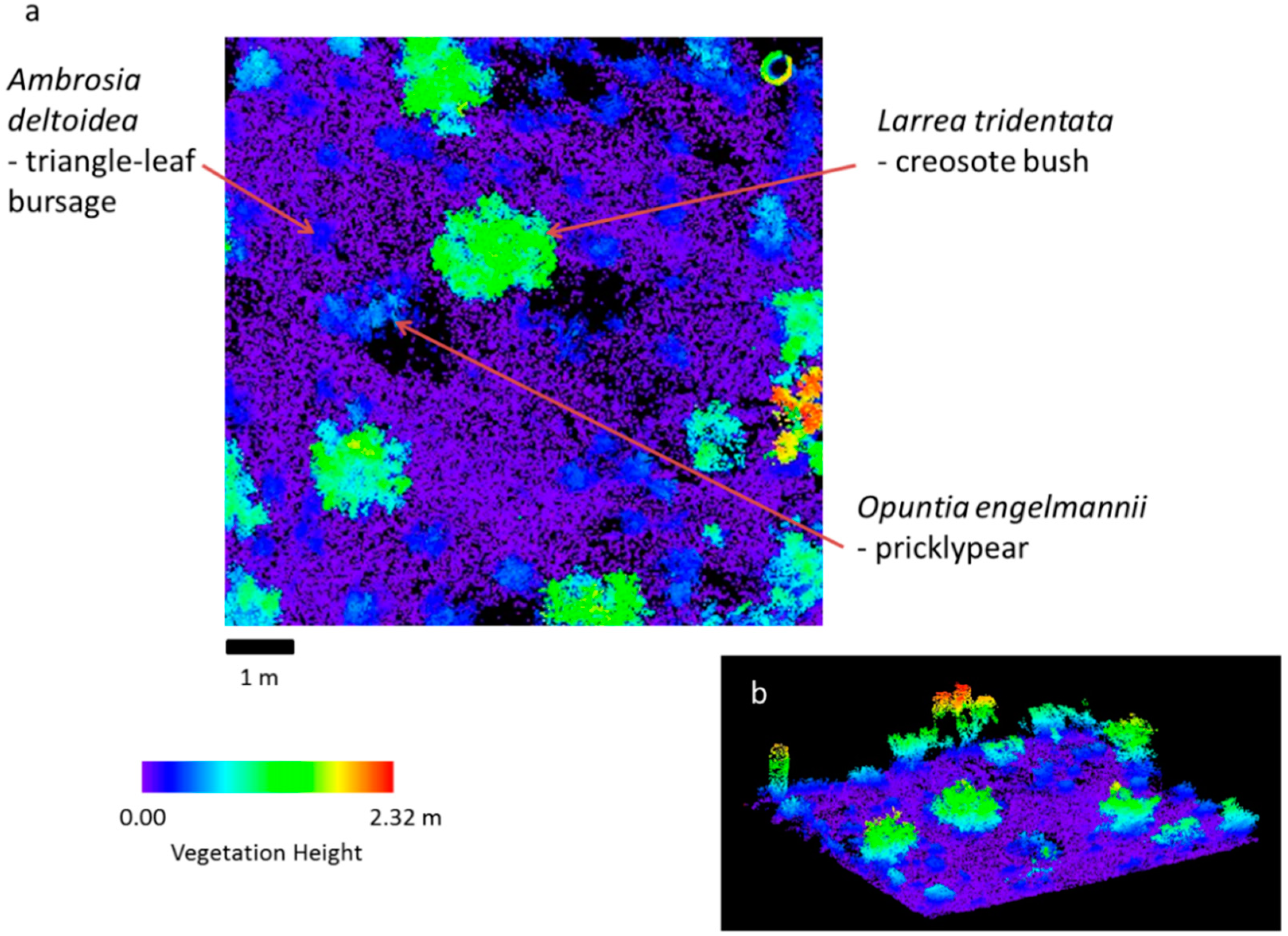
2.3. LiDAR Data Collection
| Date | RMSE (m) | |||
|---|---|---|---|---|
| X | Y | Z | Total (Mean) | |
| 11 April 2011 | 0.004 | 0.009 | 0.013 | 0.009 |
| 22 April 2011 | 0.007 | 0.008 | 0.013 | 0.010 |
| 12 May 2011 | 0.014 | 0.012 | 0.027 | 0.018 |
| 3 June 2011 | 0.007 | 0.011 | 0.008 | 0.009 |
| 21 July 2011 | 0.008 | 0.010 | 0.004 | 0.007 |
| 9 August 2011 | 0.014 | 0.014 | 0.008 | 0.012 |
| 8 September 2011 | 0.006 | 0.008 | 0.009 | 0.008 |
| 7 October 2011 | 0.020 | 0.005 | 0.011 | 0.012 |
| 23 December 2011 | 0.006 | 0.009 | 0.020 | 0.012 |
| 13 March 2012 | 0.017 | 0.009 | 0.019 | 0.015 |
| 13 March 2012 * | 0.015 | 0.009 | 0.007 | 0.010 |
| 11 May 2012 | 0.011 | 0.006 | 0.019 | 0.009 |
2.4. LiDAR Processing

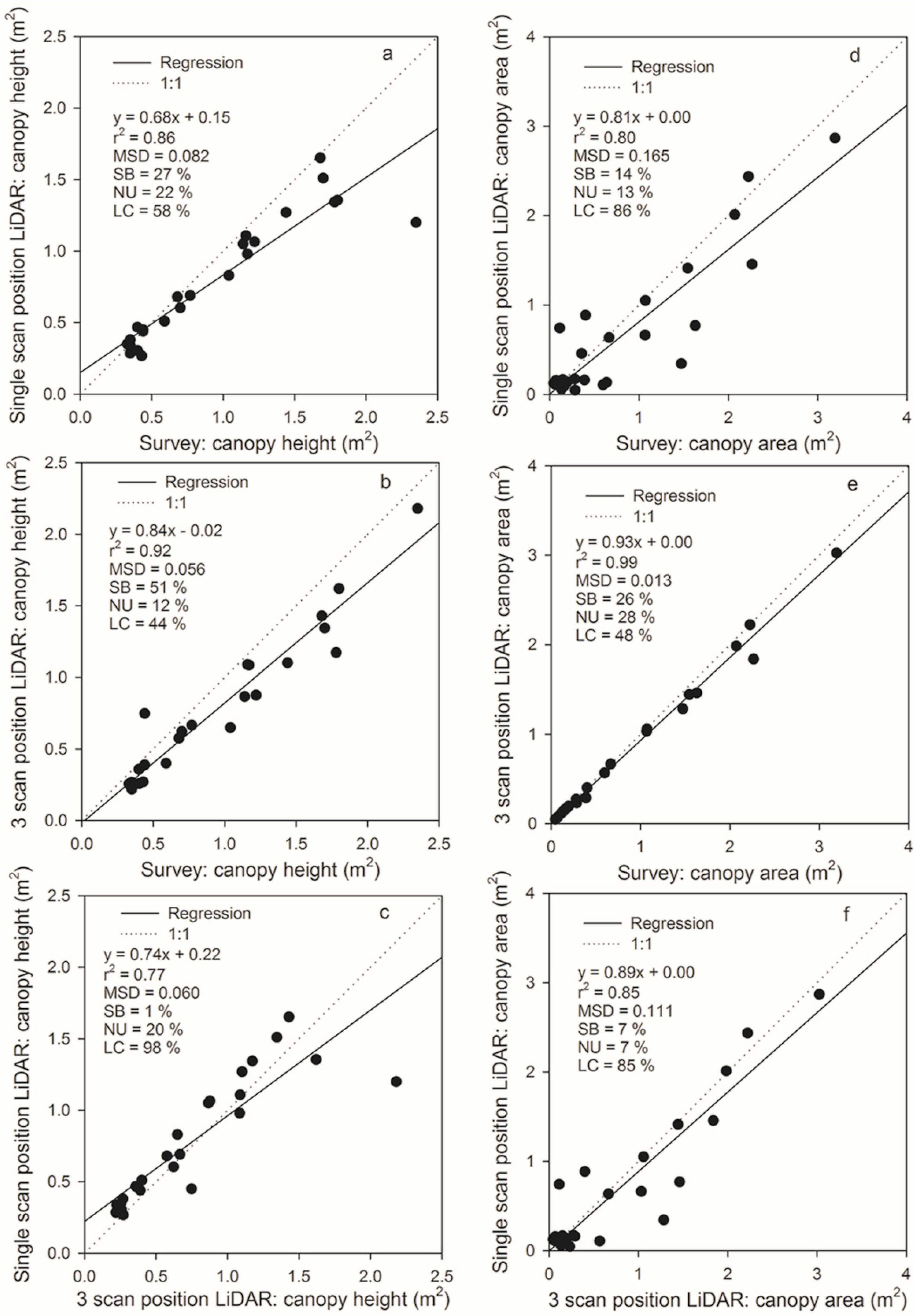
2.5. LiDAR Measurement Accuracy and Analysis of Intra-Annual Variability
3. Result
3.1. LiDAR Processing and Measurement Accuracy
3.2. Intra-Annual Precipitation and Satellite-Derived Greenness Variability


3.3. Plot-Scale Intra-Annual LiDAR Variability
3.4. Species-Specific Intra-Annual LiDAR Variability
4. Discussion

| Species | Vegetation Returns (%) | Canopy Height (m) | Canopy Area (m2) |
|---|---|---|---|
| Ambrosia deltoidea | 0.63 (0.04) * | 0.60 (0.05) | 0.53 (0.09) |
| Larrea tridentata | 0.24 (0.46) | −0.31 (0.35) | 0.43 (0.18) |
| Opuntia engelmannii | 0.40 (0.22) | 0.31 (0.35) | −0.11 (0.74) |
4.1. LiDAR Processing and Measurement Accuracy
4.2. Intra-Annual Variability
5. Conclusions
Acknowledgments
Author Contributions
Conflicts of Interest
References
- Goldberg, D.E.; Turner, R.M. Vegetation change and plant demography in permanent plots in the Sonoran Desert. Ecology 1986, 67, 695–712. [Google Scholar]
- Munson, S.M.; Webb, R.H.; Belnap, J.; Hubbard, J.A.; Swann, D.E.; Rutman, S. Forecasting climate change impacts to plant community composition in the Sonoran Desert region. Glob. Chang. Biol. 2012, 18, 1083–1095. [Google Scholar] [CrossRef]
- Webb, R.H.; DeFalco, L.A.; Esque, T.C.; Medica, P.A. A review of selected long-term ecological studies of the Mojave Desert. In Mojave Desert: Ecosystem Processes and Sustainability; Webb, R.H., Fenstermaker, L.F., Heaton, J.S., Hughson, D.L., McDonald, E.V., Miller, D.M., Eds.; University of Nevada Press: Reno, NV, USA, 2009; pp. 429–456. [Google Scholar]
- Webb, R.H.; Turner, R.M. A debt to the past: Continuing long-term and current research at the Desert Laboratory in Tucson. Desert Plants 2011, 26, 3–18. [Google Scholar]
- Canfield, R.H. Application of the line interception methods in sampling range vegetation. J. For. 1941, 39, 388–394. [Google Scholar]
- Daubenmire, R. A canopy-coverage method of vegetational analysis. Northwest Sci. 1941, 33, 43–64. [Google Scholar]
- Munson, S.M.; Webb, R.H.; Hubbard, J.A. A comparison of methods to assess long-term changes in Sonoran Desert vegetation. J. Arid Environ. 2011, 75, 1228–1231. [Google Scholar] [CrossRef]
- The Desert Laboratory Repeat Photography Collection—An Invaluable Archive Documenting Landscape Change. U.S. Geological Survey Fact Sheet 2007–3046; 2007. Available online: http://pubs.usgs.gov/fs/2007/3046/ (accessed on 9 December 2014).
- Eitel, J.U.H.; Vierling, L.A.; Long, D.S. Simultaneous measurements of plant structure and chlorophyll content in broadleaf saplings with a terrestrial laser scanner. Remote Sens. Environ. 2010, 114, 2229–2237. [Google Scholar] [CrossRef]
- Magney, T.S.; Eusden, S.A.; Eitel, J.U.H.; Logan, B.A.; Jiang, J.; Vierling, L.A. Assessing leaf photoprotective mechanisms using terrestrial LiDAR: Towards mapping canopy photosynthetic performance in three dimensions. New Phytol. 2013, 201, 344–356. [Google Scholar] [CrossRef] [PubMed]
- Ku, N.W.; Popescu, S.C.; Ansley, R.J.; Perotto-Baldivieso, H.L.; Filippi, A.M. Assessment of available rangeland woody plant biomass with a terrestrial LiDAR system. Photogram. Eng. Remote Sens. 2012, 78, 349–361. [Google Scholar] [CrossRef]
- Mitchell, J.J.; Glen, N.F.; Sankey, T.T.; Derryberry, D.R.; Anderson, M.O.; Hruska, R.C. Small-footprint LiDAR estimations of sagebrush canopy characteristics. Photogram. Eng. Remote Sens. 2011, 77, 521–530. [Google Scholar] [CrossRef]
- Popescu, S.C.; Wynne, R.H.; Nelson, R.F. Estimating plot-level tree heights with LiDAR: Local filtering with a canopy-height based variable window size. Comput. Electron. Agric. 2002, 37, 71–95. [Google Scholar] [CrossRef]
- Popescu, S.C.; Wynne, R.H. Seeing the trees in the forest: Using LiDAR and multispectral data fusion with local filtering and variable window size for estimating tree height. Photogram. Eng. Remote Sens. 2004, 70, 589–604. [Google Scholar] [CrossRef]
- Zhao, K.; Popescu, S.; Meng, X.; Pang, Y.; Agca, M. Characterizing forest canopy structure with LiDAR composite metrics and machine learning. Remote Sens. Environ. 2011, 115, 1978–1996. [Google Scholar] [CrossRef]
- Hudak, A.T.; Strand, E.K.; Vierling, L.V.; Byrne, J.; Eitel, J.U.H.; Martinuzzi, S.; Falkowski, M.J. Quantifying aboveground forest carbon pools and fluxes from repeat LiDAR surveys. Remote Sens. Environ. 2012, 123, 25–40. [Google Scholar] [CrossRef]
- Sankey, T.T.; Shrestha, R.; Sankey, J.B.; Hardegree, S.; Strand, E. LiDAR-derived estimate and uncertainty of carbon sink in successional phases of woody encroachment. J. Geophys. Res.-Biogeosci. 2013, 118, 1144–1155. [Google Scholar]
- Riaño, D.; Valladares, F.; Condés, S.; Chuvieco, E. Estimation of leaf area index and covered ground from airborne laser scanner (LiDAR) in two contrasting forests. Agric. For. Meteorol. 2004, 124, 269–275. [Google Scholar] [CrossRef]
- Arno, J.; Escola, A.; Valles, J.; Llorens, J.; Sanz, R.; Msip, J.; Palacin, J.; Rosell-Polo, J.R. Leaf area index estimation in vineyards using a ground-based LiDAR scanner. Precis. Agric. 2013, 14, 290–306. [Google Scholar] [CrossRef] [Green Version]
- Zhao, F.; Yang, X.; Schull, M.A.; Roman-Colon, M.O.; Yao, Tian; Wang, Z. Measuring effective lead area index, foliage profile, and stand height in New England forests using a fullwaveform ground-based LiDAR. Remote Sens. Environ. 2011, 115, 2954–2964. [Google Scholar] [CrossRef]
- Sankey, J.B.; Ravi, S.; Wallace, C.S.A.; Webb, R.H.; Huxman, T.E. Quantifying soil surface change in degraded drylands: Shrub encroachment and effects of fire and vegetation removal in a desert grassland. J. Geophys. Res. 2012, 117. [Google Scholar] [CrossRef]
- Sankey, J.B.; Law, D.J.; Breshears, D.D.; Munson, S.M.; Webb, R.H. Employing LiDAR to detail vegetation canopy architecture for prediction of aeolian transport. Geophys. Res. Lett. 2013, 40, 1724–1728. [Google Scholar] [CrossRef]
- Eitel, J.U.H.; Vierling, L.A.; Magney, T.S. A lightweight, low cost autonomously operating terrestrial laser scanner for quantifying and monitoring ecosystem structural dynamics. Agric. For. Meteorol. 2013, 180, 86–96. [Google Scholar] [CrossRef]
- Higgins, R.W.; Yao, Y.; Wang, X.L. Influence of the North American Monsoon system on the U.S. summer precipitation regime. J. Clim. 1997, 10, 2600–2622. [Google Scholar] [CrossRef]
- Bowers, J.E. Regeneration of triangle-leaf bursage (Ambrosia deltoidea: Asteraceae): Germination behaviour and persistent seed bank. Southwest. Nat. 2002, 47, 449–513. [Google Scholar] [CrossRef]
- Bowers, J.E. Effects of drought on shrub survival and longevity in the northern Sonoran Desert. J. Torrey Bot. Soc. 2005, 132, 421–431. [Google Scholar] [CrossRef]
- Bowers, J.E. Has climatic warming altered spring flowering date of Sonoran desert shrubs? Southwest. Nat. 2007, 52, 347–355. [Google Scholar] [CrossRef]
- Bowers, J.E. A debt to the future: Achievements of the Desert Laboratory, Tumamoc Hill, Tucson, Arizona. Desert Plants 2010, 26, 25–39. [Google Scholar]
- One Hundred and Six Years of Population and Community Dynamics of Sonoran Desert Laboratory Perennials. Available online: http://pubs.er.usgs.gov/publication/70038720 (accessed on 18 December 2014).
- Rodriguez-Buritica, S.; Raichle, H.; Webb, R.H.; Turner, R.M.; Venable, L. One hundred and six years of population and community dynamics of Sonoran Desert Laboratory perennials. Ecol. Arch. 2013, 94, 976–976. [Google Scholar] [CrossRef]
- Turner, R.M.; Brown, D.E. Sonoran desertscrub. Biotic Communities of the American Southwest-United States and Mexico. Desert Plants 1982, 4, 181–221. [Google Scholar]
- InnovMetric Software. PolyWorks V10.1 Beginner’s Guide; InnovMetric Software Inc.: Quebec, QC, Canada, 2008; p. 118. [Google Scholar]
- Evans, J.S.; Hudak, A.T.; Faux, R.; Smith, A.M.S. Discrete return LiDAR in natural resources: Recommendations for project planning, data processing, and deliverables. Remote Sens. 2009, 1, 776–794. [Google Scholar] [CrossRef]
- Streutker, D.E.; Glenn, N.F. LiDAR measurement of sagebrush steppe vegetation heights. Remote Sens. Environ. 2006, 102, 135–145. [Google Scholar] [CrossRef]
- Gauch, H.G., Jr.; Hwang, J.T.G.; Fick, G.W. Model evaluation by comparison of model-based predictions and measured values. Agron. J. 2003, 95, 1442–1446. [Google Scholar] [CrossRef]
- Solano, R.; Didan, K.; Jacobson, A.; Huete, A. MODIS Vegetation Indices (MOD13) C5-User’s Guide; The University of Arizona: Tucson, AZ, USA, 2010; p. 38. [Google Scholar]
- Szarek, S.R.; Woodhouse, R.M. Ecophysiological studies of Sonoran Desert Plants. Oecologia 1977, 28, 365–375. [Google Scholar] [CrossRef]
- Meinzer, F.C.; Rundel, P.W.; Sharifi, M.R.; Nilsen, E.T. Turgor and osmotic relations of the desert shrub Larrea tridentate. Plant Cell Environ. 1986, 9, 467–475. [Google Scholar] [CrossRef]
- Spalding, E.S. Mechanical adjustment of the saguaro (Cereus giganteus) to varying quantities of stored water. Bull. Torrey Bot. Club 1905, 32, 57–68. [Google Scholar] [CrossRef]
- Munson, S.M. Plant responses, climate pivot points, and trade-offs in water-limited ecosystems. Ecosphere 2013, 4. [Google Scholar] [CrossRef]
© 2014 by the authors; licensee MDPI, Basel, Switzerland. This article is an open access article distributed under the terms and conditions of the Creative Commons Attribution license (http://creativecommons.org/licenses/by/4.0/).
Share and Cite
Sankey, J.B.; Munson, S.M.; Webb, R.H.; Wallace, C.S.A.; Duran, C.M. Remote Sensing of Sonoran Desert Vegetation Structure and Phenology with Ground-Based LiDAR. Remote Sens. 2015, 7, 342-359. https://0-doi-org.brum.beds.ac.uk/10.3390/rs70100342
Sankey JB, Munson SM, Webb RH, Wallace CSA, Duran CM. Remote Sensing of Sonoran Desert Vegetation Structure and Phenology with Ground-Based LiDAR. Remote Sensing. 2015; 7(1):342-359. https://0-doi-org.brum.beds.ac.uk/10.3390/rs70100342
Chicago/Turabian StyleSankey, Joel B., Seth M. Munson, Robert H. Webb, Cynthia S. A. Wallace, and Cesar M. Duran. 2015. "Remote Sensing of Sonoran Desert Vegetation Structure and Phenology with Ground-Based LiDAR" Remote Sensing 7, no. 1: 342-359. https://0-doi-org.brum.beds.ac.uk/10.3390/rs70100342