Developing Superfine Water Index (SWI) for Global Water Cover Mapping Using MODIS Data

Abstract

Monitoring of water cover and shorelines at a global scale is essential for better understanding climate change consequences and modern human disturbances. The level and turbidity of the surface water, and the background objects in which they interact with, vary significantly at a global scale. The existing water indices applicable to detection and extraction of water cover at local and regional scales cannot work efficiently everywhere in the globe. In this research, a new water index called Superfine Water Index (SWI) was developed for robust detection and discrimination of the surface water at a global scale using MODIS based multispectral data. The SWI was designed in such a way that it provides high contrast between the water and non-water areas. Achieving high contrast is vital for discriminating the surface water mixed with a variety of objects. The sensitivity analysis of the SWI demonstrated its high sensitivity to the surface water compared to the existing water indices. One single-layered global mosaic of a 90-percentile SWI image was used as a master image for global water cover mapping by reducing the large volume of MODIS data available between 2012 and 2014 globally. The random walker algorithm was applied in the SWI image with the support of reference training data for the extraction and mapping of water cover. This research produced an up-to-date global water cover map of the year 2013. The performance of a new map was evaluated with a number of case studies and compared with existing maps. The supremacy of the SWI over the existing water indices, and high performance of the SWI based water map confirmed the reliability of the new water mapping methodology developed. We expect that this methodology can contribute to seasonal and annual change analysis of the global water cover as well.

1. Introduction

Water is an important resource for life on Earth. It is also crucial for agricultural and industrial production affecting the economic development of countries. However, the dramatic increase in population and industry and the unequivocal change of climate systems has put the sustainability of water resources in doubt, while a number of regions have already faced serious shortages of drinking water. On the other hand, water related disasters such as severe drought, inundation and flooding have occurred frequently in many places on Earth. The water cover at a global scale has been changing rapidly in recent decades influenced by climate-hydrological changes. The monitoring of the water cover and shorelines at a global scale is essential for better understanding climate change consequences and modern human disturbances. The near-real time monitoring of the surface water and coastlines can track water-related disasters and protect life and property. The water cover and coastline database is also important for various applications such as landscape design, infrastructure development, earthquake and tsunami hazard planning, and managing resilience and sustainability of ecosystems.

Over recent decades, a number of remote sensing techniques based on aerial photographs, optical satellite imagery, radar satellite imagery, airborne laser imagery, and airborne video imagery have been utilized for detection and extraction of coastlines/shorelines and inland water bodies. Digital photogrammetry with aerial and satellite imagery have been widely used for the monitoring of shorelines/coastlines, and detecting their temporal and spatial changes in several locations around the world [1,2,3,4,5,6,7,8,9,10,11,12,13]. Besides the optical imagery based approach, the synthetic aperture radar (SAR) based multi-polarization and multi-incidence data have also been used by many researchers for water monitoring and mapping purposes [14,15,16,17]. Not only detection and mapping of the shorelines and water cover, but validation of the satellite based estimates are equally important. The coastlines detected by multi-temporal satellite imagery have been well verified by a number of studies using topographic, nautical, water level surveys, and near-ground photography [18,19]. Remote sensing video systems are another tool for coastline change detection used by some researchers [20,21,22,23]. Airborne Lidar is suggested for improved detection and monitoring of coastlines [24,25,26,27]. The edge detection technique with the radar and optical satellite images have been described as a more precise method for extracting shorelines/coastlines [28,29]. Pekel et al. [30] used HSV transformation of mid-near infrared, near infrared, and red bands of MODIS multi-spectral time series data for developing automated algorithms for near real-time water surface detection, and characterization of their spatial and temporal dynamics. Several researchers have reported better target identification and extraction by the HSV (Hue, Saturation, and Value) color model than by the RGB model [30,31,32]. Verpoorter et al. [33] produced high-resolution global database of lakes using Landsat 7 data. Feng et al. [34] prepared global, high-resolution (30-m) inland water body dataset for 2000 using topographic-spectral classification algorithm.

The Normalized Difference Water Index (NDWI) [35] using the reflected near infrared radiation and visible green light was developed to delineate and extract open water features in remotely-sensed digital imagery (Equation (1)).

$$NDWI= \frac{Green-Nir}{Green+ Nir}$$

(1)

Besides from the extraction and mapping of water bodies, the NDWI has been widely used for many water related researches including detection of flood inundation and flood mapping from space based or airborne imagery [36,37,38,39]. The NDWI has also been used for mapping of vegetation water contents [40,41].

Xu [42] modified the NDWI by substituting shortwave infrared band (band 5) of Landsat TM for the near infrared band used in the NDWI to suppress the false positive errors from built-up land as well as vegetation and soil. The Modified Normalized Water Index (MNDWI) by this approach is shown in Equation (2).

$$MNDWI= \frac{Green-Swir}{Green+ Swir}$$

(2)

Feyisa et al. [43] proposed Automated Water Extraction Index (AWEI) by enhancing spectral contrast of Landsat TM data and assigning an optimal threshold value for accurate classification of surface water bodies (Equation (3)).

$$\text{AWEI}=4\times \left(\text{Green}-\text{Mir}\right)-\left(0.25\times \text{ Nir }+2.75\times \text{ Swir}\right)$$

(3)

Ayana et al. [44] proposed Enhanced Water Index (EWI) by combing the Normalized Difference Vegetation Index (NDVI) with the Normalized Difference Water Index (NDWI) for improving water extraction accuracy in the presence of various environmental noises using a stable threshold (Equation (4)). Unlike the NDWI, MNDWI, and AWEI, the EWI provides discrete mask of the surface water and non-water, but not the continuous measure of the wateriness of the land surface.

$$\text{EWI}=\text{ if }\left(\text{NDVI}<0\text{ and NDWI}>0,\prime \text{water}\prime \text{ else }\prime \text{land}\prime \right)$$

(4)

However, most of the studies on water cover detection, extraction, and mapping were carried out at local to regional scale, and limited studies were conducted at a global level. The databases that provide ocean and inland water cover at global scale are as follows: Global Self-consistent, Hierarchical, High-resolution Geography database 2015 (GSHHG; [45]), and MODIS land-water mask product 2009 (MOD44W; [46,47], MODIS Land Cover Type Product 2012 (MCD12Q1 v5.1; [48]), GLCNMO 2008 [49], and ESA GlobCover 2009 [50].

The GSHHG database provides geography datasets for world shorelines, rivers, and borders at five resolutions. The database is organized into multiple hierarchical and classification levels. In this database, the polygons representing land–ocean boundaries, and the shorelines related to the land-lake and land-river boundaries can be separated. The early GSHHG database was constructed from two well-known and public domain datasets: the World Data Bank II [51] containing coastlines, lakes, political boundaries, and river; and the World Vector Shoreline [52] containing the shorelines along the ocean and land boundary. The line segments and polygons from these two data sources were processed by removing duplicates and outliers, and combined with each other to obtain the closed and high-resolution polygons [45]. The latest product results from continuous revision since the early processing.

The MODIS land-water mask (MOD44W) product provides the mask between land and water including both the inland water bodies such as rivers and lakes, and ocean. However, it does not distinguish between the ocean and inland water bodies, and serves both the ocean and inland water bodies as a single water product. This product has a long history of development. The MOD44W product was developed through improvement of the Shuttle Radar Topography Mission’s (SRTM) land-water mask with MODIS Nadir Bidirectional Reflectance Distribution Function (BRDF)-Adjusted Reflectance (NBAR) product, MODIS land cover product, and MODIS–based Mosaic of Antarctica. This product is available at 250-m spatial resolution raster grids.

The MODIS Land Cover Type Product under the International Geosphere-Biosphere Programme (IGBP) classification [53] system classifies the cover types using an ensemble supervised classification algorithm (decision tree) complemented by the training data from 1860 sites distributed across the Earth’s land areas [48].

The Global Land Cover by National Mapping Organizations (GLCNMO) classifies the water cover based on tasseled cap transformation [54] of the MODIS seven bands’ data by referencing with MODIS land-water mask product (MOD44W) [49].

The GlobCover 2009 by European Space Agency (ESA) based on Medium Resolution Imaging Spectrometer (MERIS) apply the ISODATA clustering method and labeling by reference data as the basic method.

The water cover mapping at global scale is challenging because the level and turbidity of the surface water and the background objects in which they interact with vary significantly. The existing water indices applicable to detection and extraction of water cover at local and regional scales cannot work efficiently everywhere in the globe. In this research, a new methodology was developed for robust detection and mapping of the marine and continental surface water solely based on MODIS based multispectral data. The spectral index based mapping approach was chosen for its simplicity, cost-effectiveness, and faster reproducibility.

2. Methodology

2.1. Proposal of Superfine Water Index (SWI)

Discriminating the water bodies from dense vegetation and snowy background are difficult with the Normalized Difference Water Index (NDWI). Potential of NDWI based discrimination and extraction of the water cover becomes worse particularly in northern, higher latitudes where the surface water bodies are covered by temporary snowfall, and in the vegetative regions where the shallow water bodies are mixed with the vegetation. The Modified Normalized Difference Water Index (MNDWI) and Automated Water Extraction Index (AWEI) that use short wave infrared band are more susceptible to snow, and cannot work efficiently in snowy regions.

In this research, a new spectral index called “Superfine Water Index (SWI)” has been developed for better detection and discrimination of the surface water everywhere in the globe. The SWI is derived by replacing the “Green” in the NDWI with the ‘Saturation (Sat)’ obtained from the HSV (Hue-Saturation-Value) transformation of the RGB composite made up of red (R), green (G), and blue (B) bands of the MODIS data. The formulation of the SWI is shown in Equation (5).

$$SWI= \frac{Sa{t}_{\left(RGB\right)} - 7 \times Nir}{Sa{t}_{\left(RGB\right)}+ 7 \times Nir}$$

(5)

The SWI provides very high contrast between the surface water and non-water cover types including the snow and vegetation. The coefficient on the near infrared reflectance in Equation (5) was introduced in such a way that it provides high contrast between the saturation values and near infrared reflectance of the non-water areas, whereas, at the same time, the raised near infrared reflectance does not reach the saturation values of the water areas. The coefficient of 7.0 was used in this research because raising the near infrared reflectance up to that level did not interfere with the saturation values of the water areas everywhere in the globe while tuning up the contrast of the non-water areas well. The normalization of the difference between the saturation (Sat) and near infrared (Nir) is used to standardize the dynamic range of the SWI between −1 and 1.

2.2. Calculation of Water Indices

The MODIS based 8-day Level 3 Global 500-m Nadir Bidirectional Reflectance Distribution Function (BRDF)-Adjusted Reflectance (NBAR) product (MCD43A4; [55]) data between January 2012 and December 2014 were obtained from the U.S. Geological Survey (USGS). The MCD43A4 product has been validated over a number of land cover types by several researchers e.g., [56,57,58,59,60,61] granting wider scientific usage. We used 3-years data from 2012–2014 so as to minimize the void data pixels due to cloudy pixels represented by the year 2013. For each time period, the Superfine Water Index (SWI) along with other three existing water indices: Normalized Difference Water Index (NDWI), Modified Normalized Difference Water Index (MNDWI), and Automated Water Extraction Index (AWEI) were calculated. For facilitating further image processing, the water indices were converted into 8-bit unsigned integers ranging between 0 and 255.

The SWI values are proportional to the wateriness of the surface, i.e., the larger the amount of surface water, the higher the index values. However, the amount of surface water varies with time; for instance, the same area full of water in the wet season may be completely dry in the arid season. In this research, we used maximum extent of wateriness observed over a year avoiding temporary flooding. Therefore, we computed 90-percentile values from the stack of eight-day period water index images while the visual interpretation confirmed that 100-percentile values were contaminated by the signals from temporary flooding. The pixels still having the void pixels were filled by replacing the no-data values from another MODIS 8-day surface reflectance product (MOD09A1 and MYD09A1) based SWI values calculated using similar method. The computation of the percentile values reduced the big volume (900 Gigabytes) of data into a tiny single-layered final image (about 1 Gigabyte).

2.3. Evaluating SWI with Other Indices

Three land surface types from different locations were chosen for evaluating the water indices: (i) snowy region dominated by winter snowfall, (ii) relatively dry region dominated by bare soil, and (iii) wet region dominated by dense forests. The selected region of interest (ROI) in snowy (7,259,280 km²), dry (601,804 km²), and wet (2,603,154 km²) regions are very large and they include a variety of background objects. The location map of these three ROIs are displayed in Figure 1.

Figure 1. The location map of three regions of interest (ROIs) used for evaluating the water indices, and eight sites used for specific case studies.

Figure 1. The location map of three regions of interest (ROIs) used for evaluating the water indices, and eight sites used for specific case studies.

For each ROI, all MODIS scenes available between January 2012 and December 2014 were processed to create true color (RGB) composite images using 25-percentile values. The gap-free 90-percentile composite of the SWI image was interactively traced over the true color composite images, and water pixels were visually extracted by fixing the suitable threshold value between the water and non-water pixels. Though this procedure was time-consuming, water cover map capturing finer details of the surface water was obtained. This map was used as the reference map for evaluating the water indices. Though the reference map relied on the SWI index, this map was constructed by a visual interpretation technique, and therefore this map should not bias the comparison of the water indices. The SWI was used only to capture finer details of the water bodies while other alternatives were not available.

The sensitivity of the water indices to water cover was analyzed by preparing sample data of different sizes in each region of interest (ROI). For snowy region, the whole image of 8058 × 4203 pixels was divided into regular blocks of nine different sizes ranging from 16 × 8 pixels (249,001 samples) to 161 × 84 pixels (2401 samples). For each block, the average values of water indices and percentage water cover were calculated. For the dry region, the whole image of 2489 × 1111 pixels was divided into 9801 sample blocks with a block of 25 × 11 pixels. Similarly, for the wet region, the whole image of 4420 × 2738 pixels was divided into 89,401 sample blocks with a block of 15 × 9 pixels. The 90-percentile composite image of the water indices was used for the sensitivity analysis. The linear regression method with Coefficient of Determination (R²) and Root Mean Square Error (RMSE) were used to account for the relationship between the dependent variable (water indices) and independent variable (water cover).

In addition to the sensitivity analysis of the water indices, the monthly variation of the green, near infrared, saturation, and SWI were analyzed for each ROI. For this purpose, the sample blocks established in previous sensitivity analysis were separated into water and non-water blocks. The blocks larger than 75% water cover were used as the water areas; whereas the blocks smaller than 25% water cover were used as the non-water areas. This deliberate threshold for the water and non-water blocks were used to obtain a large number of samples falling in both groups. For snowy regions, we obtained 4755 blocks of water areas and 78,767 blocks of non-water areas allowing random selection of 4000 sample blocks for each of the groups. For dry regions, random sampling of 150 blocks for each of the water and non-water areas out of total 160 water and 9171 non-water blocks were used. In wet regions, random sampling of 950 blocks out of a total 953 water and 86,208 non-water blocks was done. Using all the MODIS (MCD43A4) scenes available between January 2012 and December 2014, monthly median composite images were prepared; and mean values of the green, near infrared, saturation, and SWI for each block were calculated.

2.4. Extraction and Mapping of Water Cover

The coastlines can be represented in terms of highest water line, mean high water line, or mean sea level. However, highest water line is the preferred reference for photography and photo interpretation based techniques [62,63]. In this research, the coastlines and inland water bodies were extracted based on the highest water extent approach avoiding temporary flooding since we used the 90-percentile Superfine Water Index (SWI) image.

The extraction and mapping of the water cover was supported by reference data collected using Google Earth images with visual interpretation and expert knowledge. For each of the continental non-water and water areas, 500 reference polygons were collected. In addition, 200 lines along the coastlines for each of the coastal ocean and coastal land 500-m adjacent to the coastlines were also collected. The ocean very far from the coastlines are already labeled as no-data in MODIS data, and mapping is not necessary there. For each of the continental water and non-water areas, we extracted 30,000 points randomly that fall inside the polygon out of 500 polygons; whereas for each of the coastal ocean and land areas, we extracted 5,000 points randomly that touch the line out of 200 lines. Out of 35,000 points for each of the water and non-water areas, 22,500 points were used for mapping; whereas 12,500 points were used for validation. The 70,000 reference points used in the research are displayed in Figure 2.

The reference polygons and lines were collected from large homogenous regions which did not show significant changes over the available time-series images in Google Earth between 2012 and 2014. The Google Earth serves as an interactive playground for accessing geo-spatial information by providing time-series of massive satellite imagery of very high spatial resolution. There is not another feasible and appropriate technology rather than the Google Earth for collecting the reference data for global mapping.

Figure 2. Distribution of the reference data belonging to the water and non-water areas used in the research.

Figure 2. Distribution of the reference data belonging to the water and non-water areas used in the research.

We applied random walker algorithm [64] in 90-percentile Superfine Water Index (SWI) image for the extraction of water pixels. The random walker algorithm is a graph based image segmentation technique that uses each pixel as a node which is connected to neighboring pixels by edges, and the edges are weighted to reflect the similarity between the pixels. This algorithm requires a number of pixels with known labels called seeds. Given a small number of seeds, one can analytically and quickly determine the probability that a random walker starting at each unlabeled pixel will first reach one of the pre-labeled pixels. By assigning each pixel to the label for which the greatest probability is calculated, a high-quality image segmentation could be obtained [64]. The application of the random walker algorithm with the SWI image simplified the overall mapping procedure since both the image segmentation and classification could be done simultaneously and automatically in this method. The training data collected for each of the water (coastal and continental) and non-water (coastal and continental) class were used to supply the seeds as the pre-labeled pixels for running the random walker algorithm. The segmentation result of the random walker algorithm was used to extract the water pixels from the background of non-water pixels. To avoid the bias related to placement of the seed points, the segmentation procedure was separately carried out for each region of 30° longitudes by 30° latitudes, and the extracted results were finally merged together to produce a global binary map of the water cover. The inland water bodies with diverse water levels and turbidity are different to the coastal water with a variety of shore objects. Therefore, the training data from both the coastal and continental water areas were used for the extraction of water cover.

2.5. Performance Analysis

The performance of SWI based water cover map was examined in a number of sites consisting of a variety of background objects and turbidity of surface water. The locations of these sites used for specific case studies are shown in Figure 1. The true-color (RGB) composite images using 25-percentile values of the MODIS (MCD43A4) data available between January 2012 and December 2014 were prepared as the reference images for examining the SWI based water cover maps.

The water cover map produced in this research was also compared with five existing global maps: Global Self-consistent, Hierarchical, High-resolution Geography (GSHHG) database, MODIS land-water mask product (MOD44W, 2001 and 2009), MODIS Land Cover Type Product (MCD12Q1 v5.1, 2012), Global Land Cover by National Mapping Organizations (GLCNMO v2.0, 2008), and European Space Agency’s GlobCover 2009. The variation of percentage water cover estimated by each map with respect to latitudes at 10° interval was computed by counting all the water pixels. The confusion matrix was calculated to assess the accuracy of the water cover map produced using 12,500 validation points for each of the water and non-water areas.

3. Results and Discussion

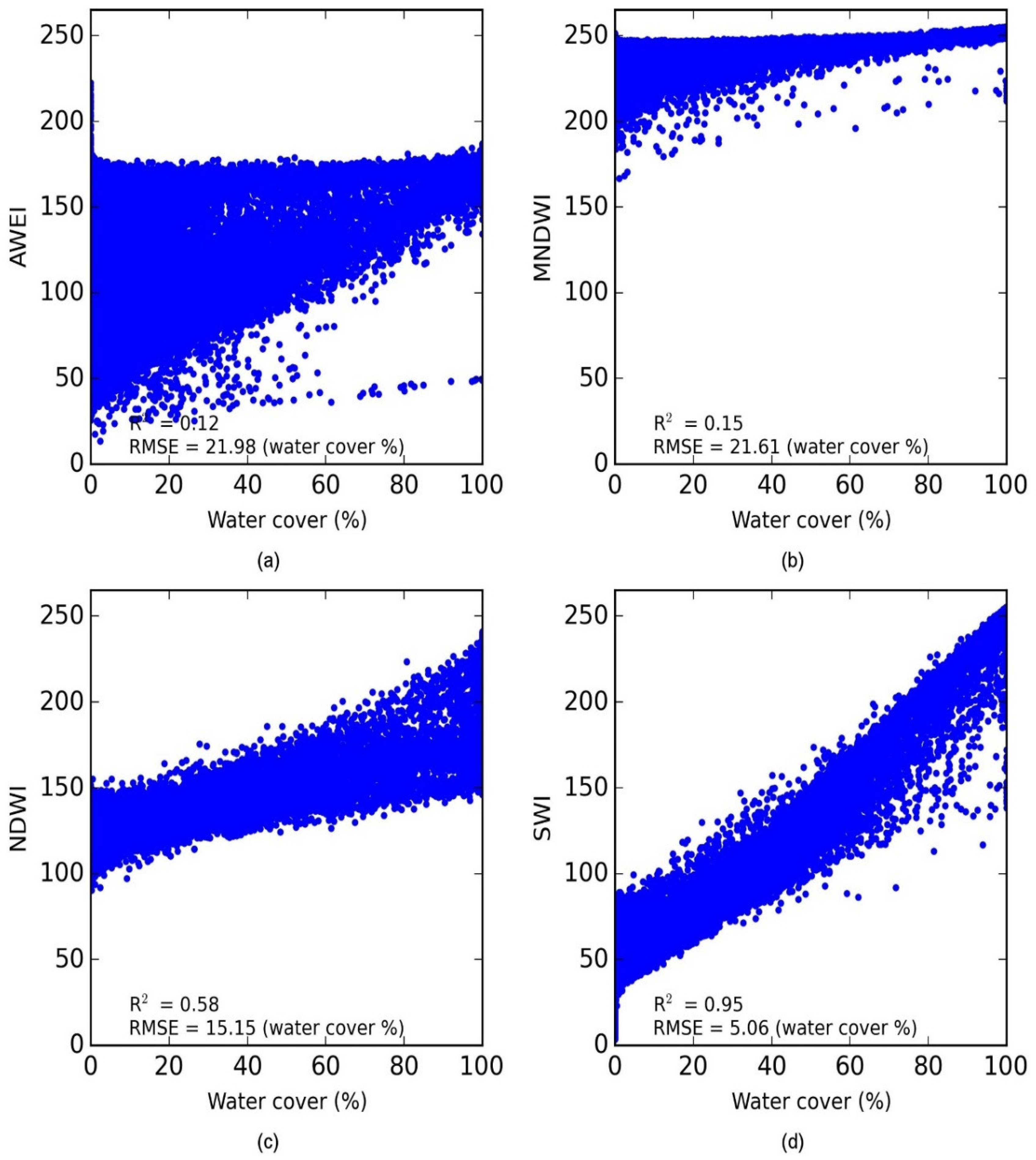
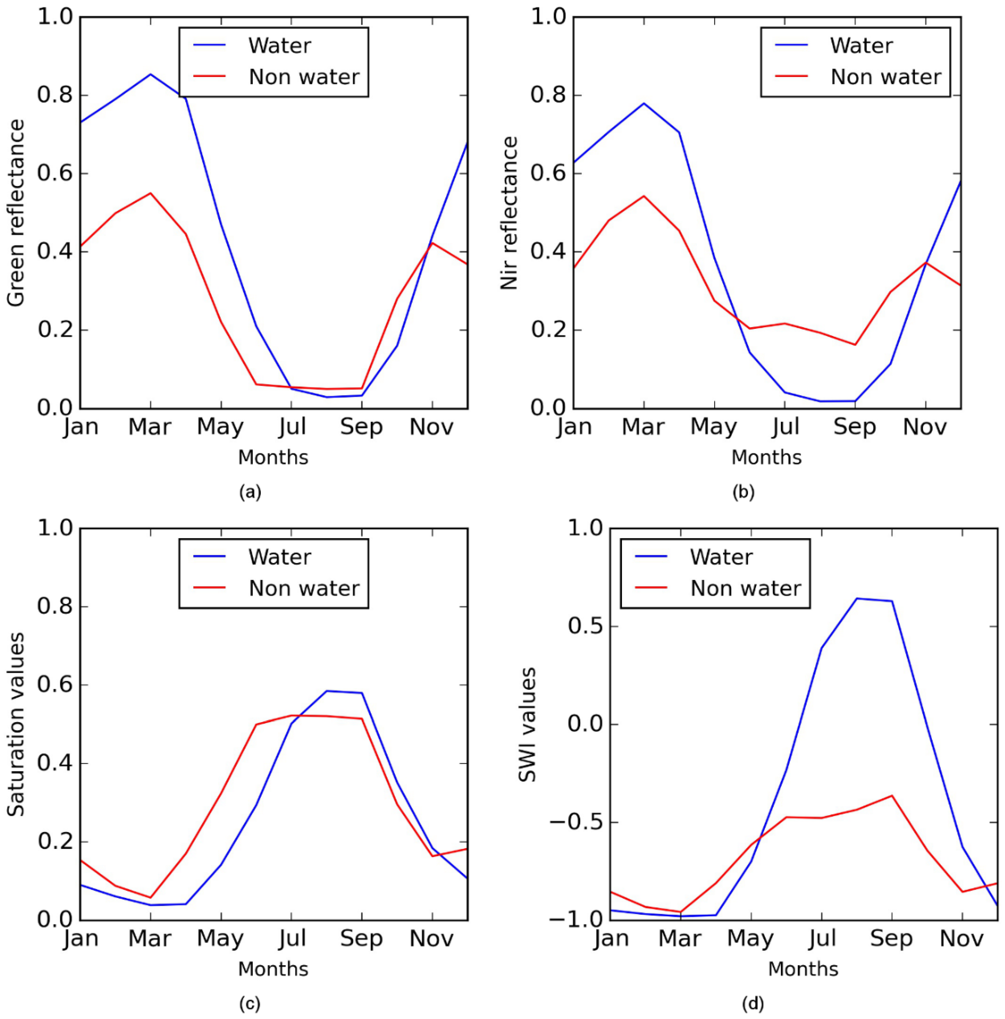
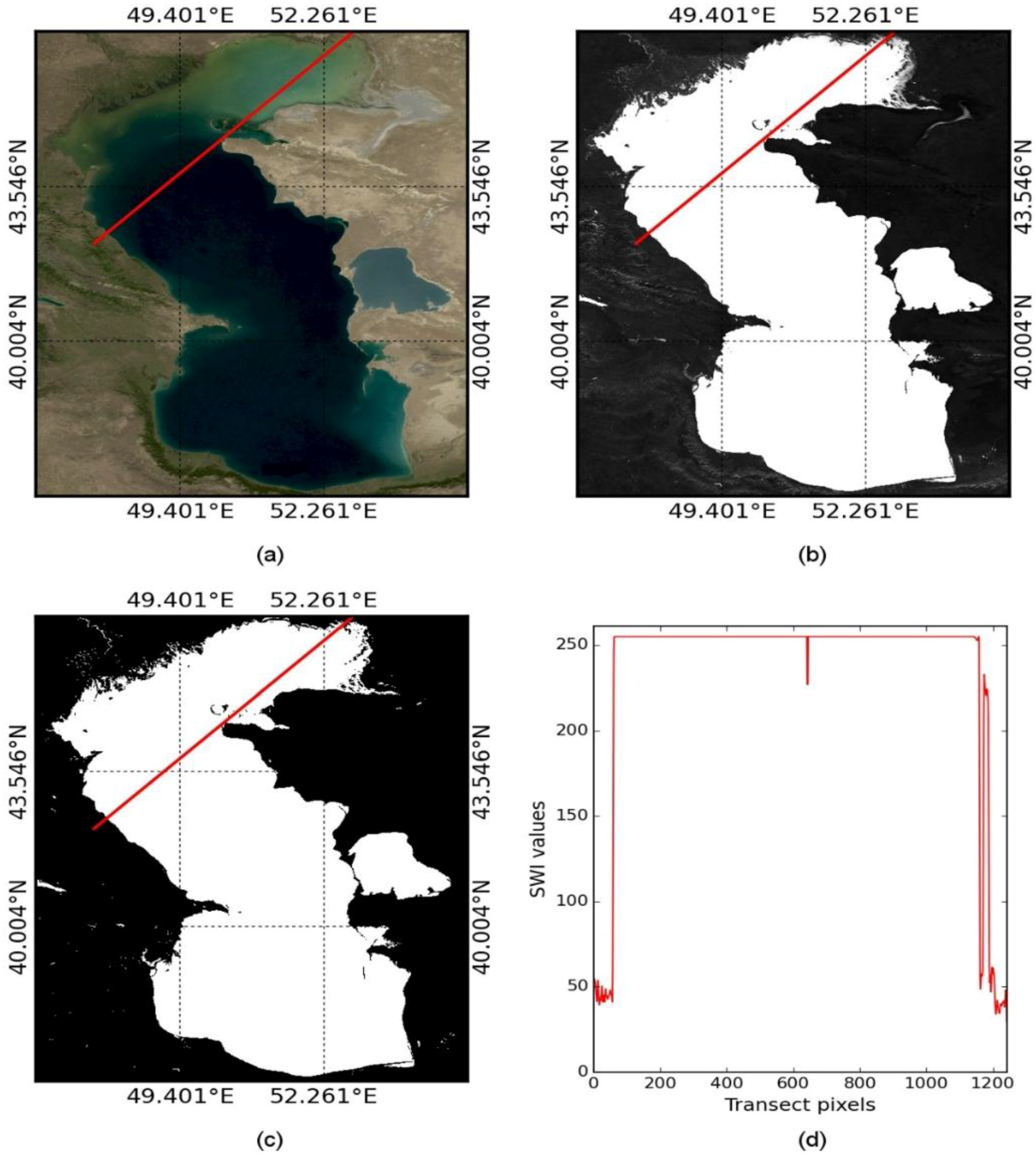
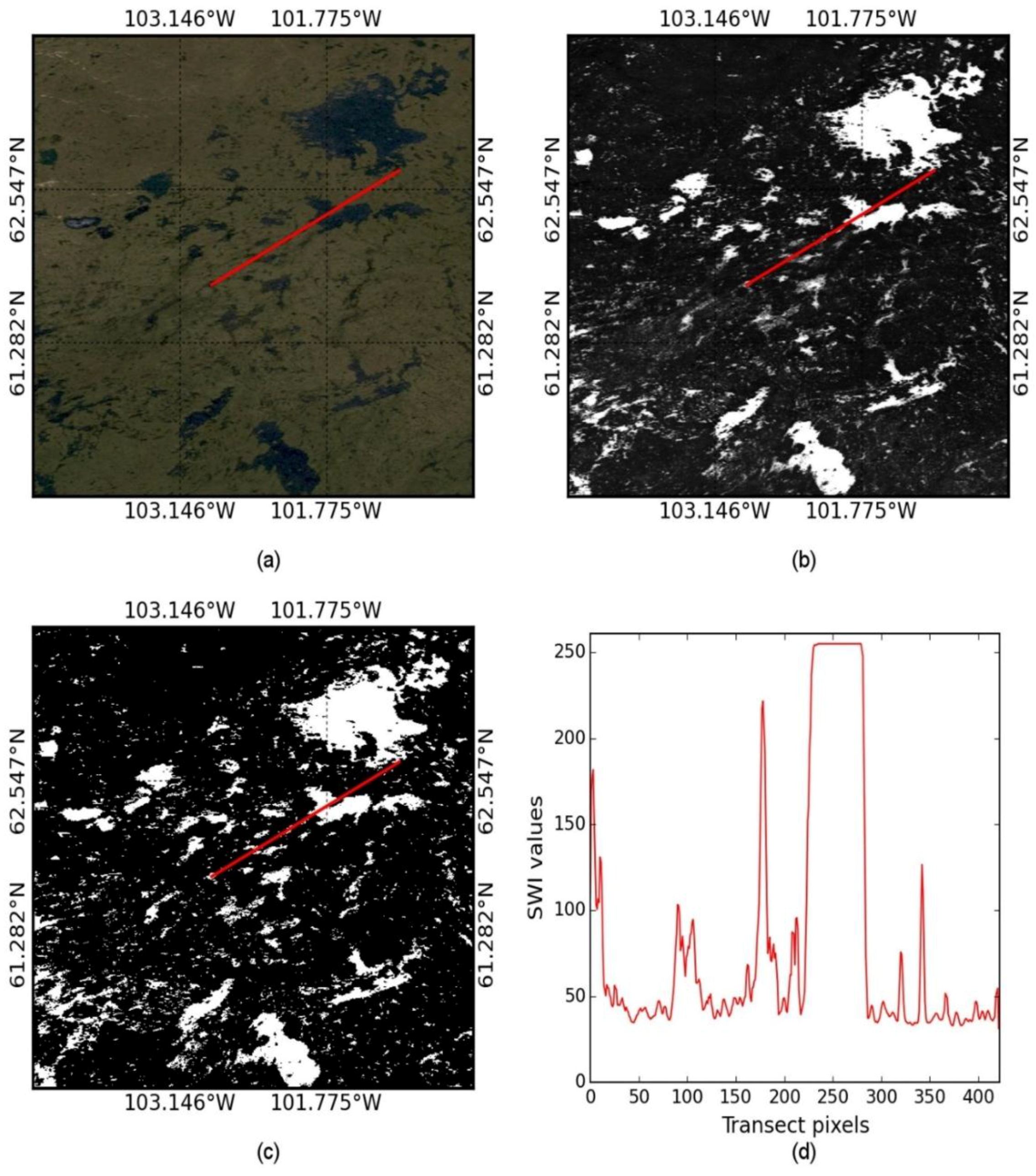
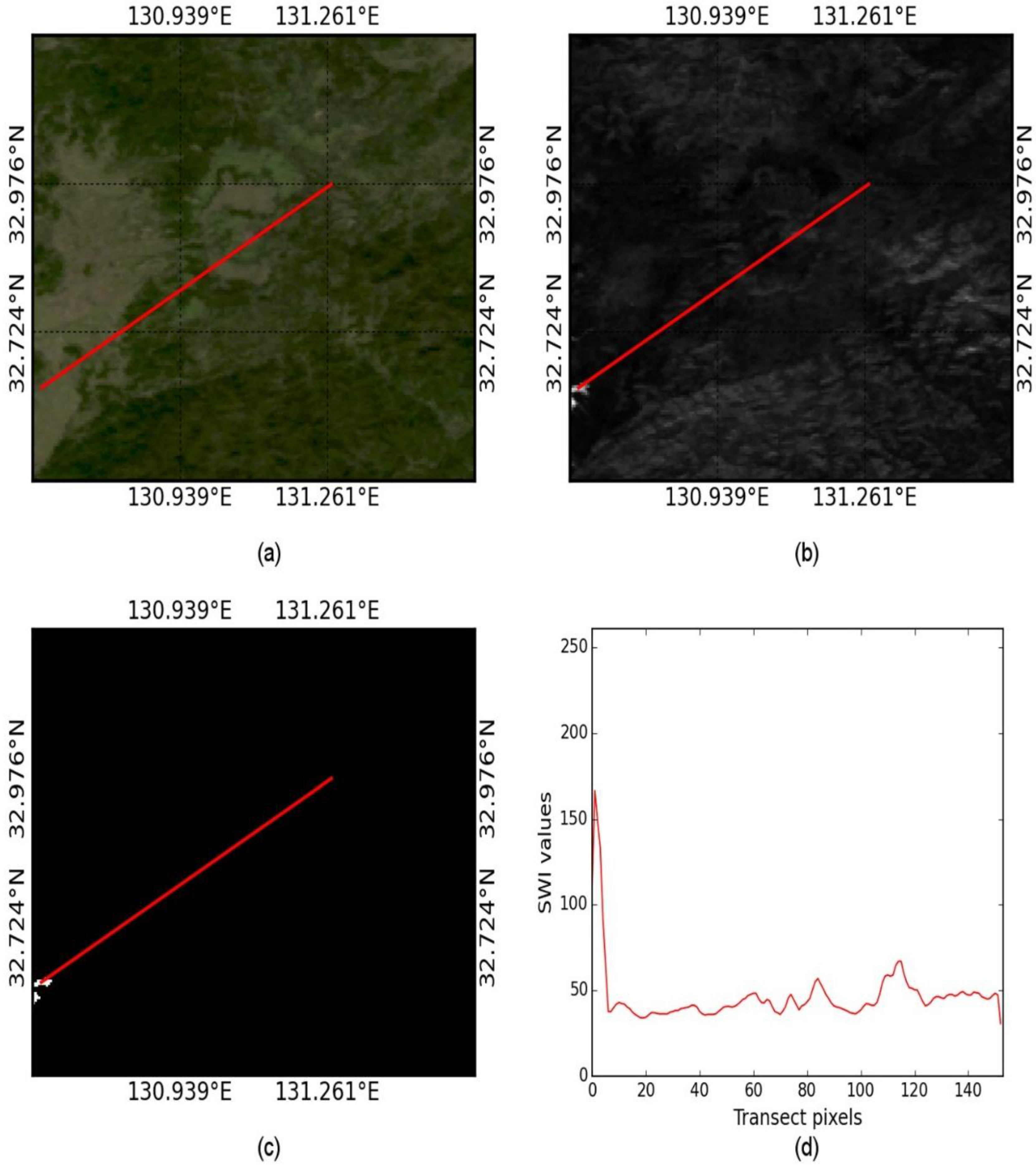
3.1. Performance of SWI in Snowy Regions

The reference water map of the snowy region is shown in Figure 3e. The visual interpretation of the five water index images with the reference water map in Figure 3 demonstrates that only the Superfine Water Index (SWI) and Normalized Difference Water Index (NDWI) images have correctly captured the details of water bodies, whereas the Automated Water Extraction Index (AWEI) and Modified Normalized Difference Water Index (MNDWI) have failed.

Figure 4 shows the relationship between the water cover and the water indices using 89,401 samples. As shown in Figure 3, the SWI performed best (R² = 0.95, RMSE = 5.06) followed by the NDWI (R² = 0.58, RMSE = 15.15). The MNDWI and AWEI could not correctly explain the variation of water cover. The short wave infrared is affected by the snow, and therefore any index using the short wave infrared did not work in the snowy region.

The results did not vary significantly by increasing or decreasing the sample sizes; therefore, the analyses using a single set of samples are displayed and discussed for all regions.

The monthly variation of the green, near infrared, saturation, and SWI in this snowy region are shown in Figure 5.

As shown in Figure 5, both the green and near infrared reflectance of the water areas showed a similar trend of variation though it was slightly different for non-water areas. However, the saturation of both the water and non-water areas showed different trends of variation than the near infrared reflectance. The SWI based on the saturation and near infrared showed high contrast between the water and non-water areas for most of the months.

Figure 3. Plotting of four water indices and water cover map in a snowy region: (a) Automated Water Extraction Index (AWEI), (b) Modified Normalized Difference Water Index (MNDWI), (c) Normalized Difference Water Index (NDWI), (d) Superfine Water Index (SWI), (e) Reference water cover map.

Figure 3. Plotting of four water indices and water cover map in a snowy region: (a) Automated Water Extraction Index (AWEI), (b) Modified Normalized Difference Water Index (MNDWI), (c) Normalized Difference Water Index (NDWI), (d) Superfine Water Index (SWI), (e) Reference water cover map.

Figure 4. The sensitivity of different water indices to the water cover in a snowy region: (a) Automated Water Extraction Index (AWEI) vs. water cover, (b) Modified Normalized Difference Water Index (MNDWI) vs. water cover, (c) Normalized Difference Water Index (NDWI) vs. water cover, (d) Superfine Water Index (SWI) vs. water cover.

Figure 4. The sensitivity of different water indices to the water cover in a snowy region: (a) Automated Water Extraction Index (AWEI) vs. water cover, (b) Modified Normalized Difference Water Index (MNDWI) vs. water cover, (c) Normalized Difference Water Index (NDWI) vs. water cover, (d) Superfine Water Index (SWI) vs. water cover.

Figure 5. Monthly variation of different parameters over the water and non-water areas in a snowy region: (a) Green reflectance, (b) Near infrared reflectance, (c) Saturation values, (d) Superfine Water Index (SWI) values

Figure 5. Monthly variation of different parameters over the water and non-water areas in a snowy region: (a) Green reflectance, (b) Near infrared reflectance, (c) Saturation values, (d) Superfine Water Index (SWI) values

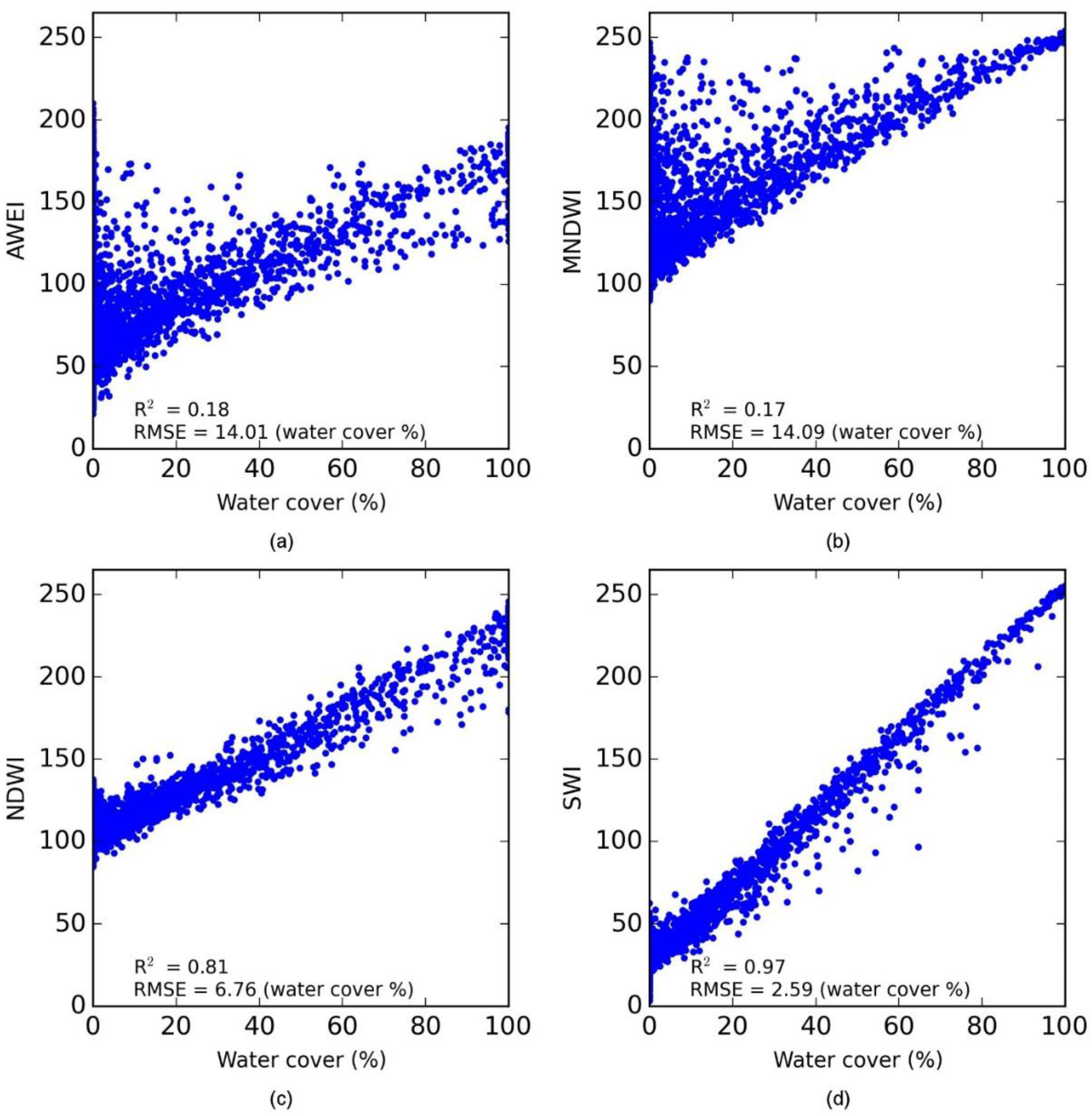
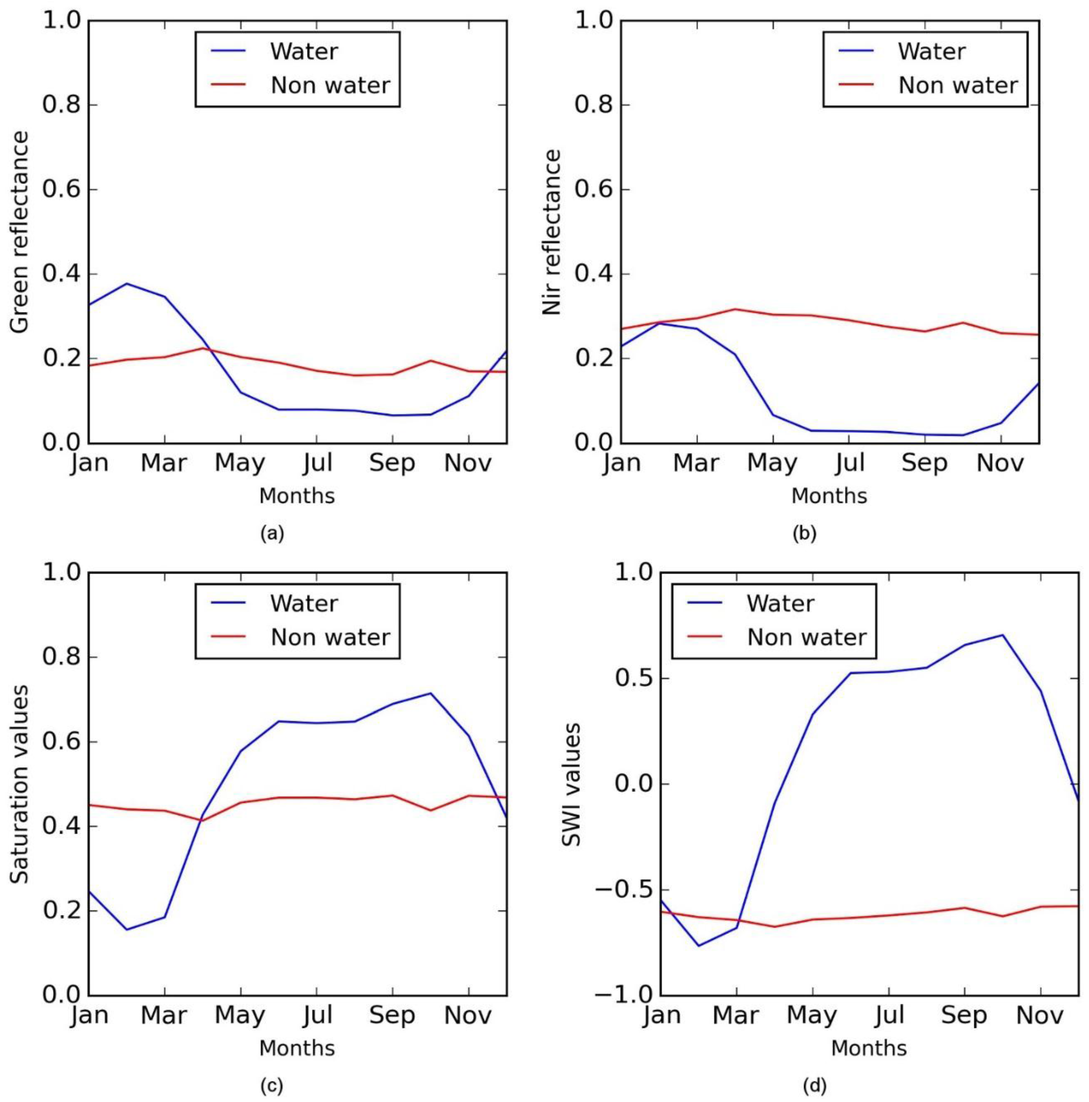
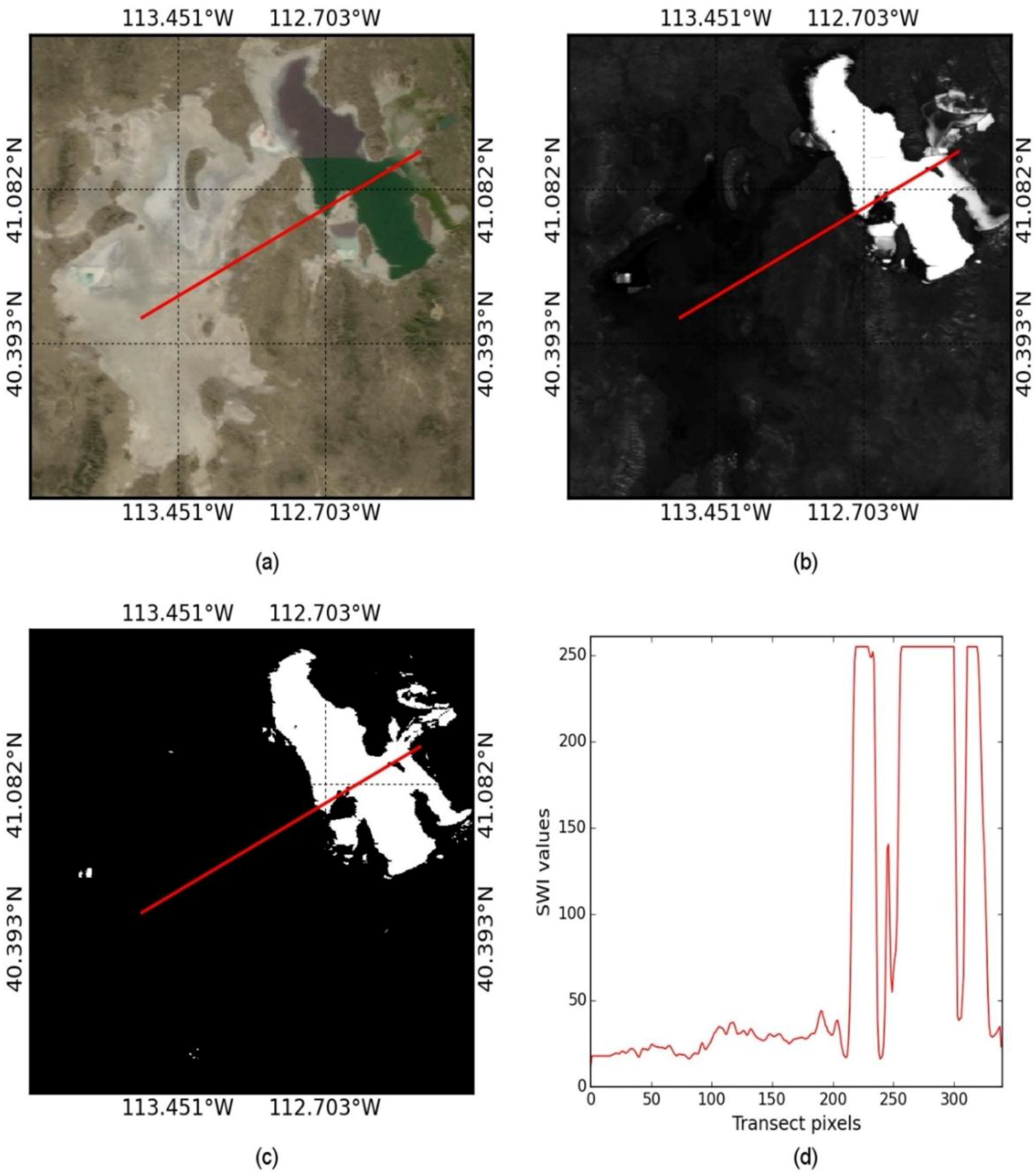
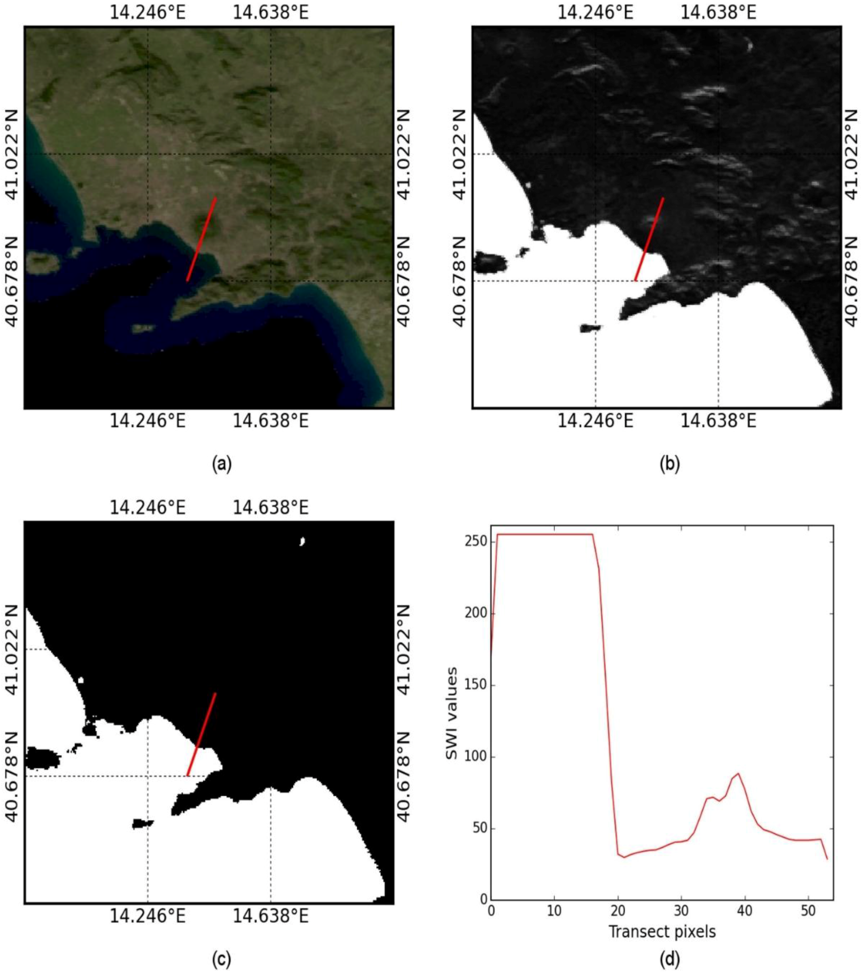
3.2. Performance of SWI in Dry Regions

The reference water map of the dry region is shown in Figure 6 along with four different water index images.

In the dry region, all the indices showed higher sensitivity to the water cover than in the snowy region (Figure 7). Nevertheless, the SWI established the strongest relationship (R² = 0.97, RMSE = 2.59) with the water cover compared to any existing indices. Among the existing indices, the NDWI was best (R² = 0.81, RMSE = 6.76). Though the detail of water bodies was not captured by the NDWI in the snowy region, it has estimated the water cover well in the dry region. This dry region also is not completely free from snow. The short wave infrared based water indices (MNDWI and AWEI) did not work very well.

Figure 6. Plotting of four water indices and water cover map in a dry region: (a) Automated Water Extraction Index (AWEI), (b) Modified Normalized Difference Water Index (MNDWI), (c) Normalized Difference Water Index (NDWI), (d) Superfine Water Index (SWI), (e) Reference water cover map.

Figure 6. Plotting of four water indices and water cover map in a dry region: (a) Automated Water Extraction Index (AWEI), (b) Modified Normalized Difference Water Index (MNDWI), (c) Normalized Difference Water Index (NDWI), (d) Superfine Water Index (SWI), (e) Reference water cover map.

Figure 7. The sensitivity of different water indices to the water cover in a dry region: (a) Automated Water Extraction Index (AWEI) vs. water cover, (b) Modified Normalized Difference Water Index (MNDWI) vs. water cover, (c) Normalized Difference Water Index (NDWI) vs. water cover, (d) Superfine Water Index (SWI) vs. water cover.

Figure 7. The sensitivity of different water indices to the water cover in a dry region: (a) Automated Water Extraction Index (AWEI) vs. water cover, (b) Modified Normalized Difference Water Index (MNDWI) vs. water cover, (c) Normalized Difference Water Index (NDWI) vs. water cover, (d) Superfine Water Index (SWI) vs. water cover.

The monthly variation of the green, near infrared, saturation, and SWI over the water and non-water areas in a dry region is shown in Figure 8.

Though both the green and near infrared bands showed a similar trend of variation over the year, for the water areas, the green reflectance was slightly larger than the near infrared reflectance. The saturation values showed different trends of variation than the near infrared reflectance for the water areas. The SWI provided high contrast between the water and non-water areas.

The green and near infrared reflectance observed in Figure 5 in the snowy region is dramatically higher than in Figure 8 in the dry region. In the presence of snow, not only the green reflectance but also the near infrared reflectance further reduced the discriminability between the water and non-water areas.

Figure 8. Monthly variation of different parameters over the water and non-water areas in a dry region: (a) Green reflectance, (b) Near infrared reflectance, (c) Saturation values, (d) Superfine Water Index (SWI) values.

Figure 8. Monthly variation of different parameters over the water and non-water areas in a dry region: (a) Green reflectance, (b) Near infrared reflectance, (c) Saturation values, (d) Superfine Water Index (SWI) values.

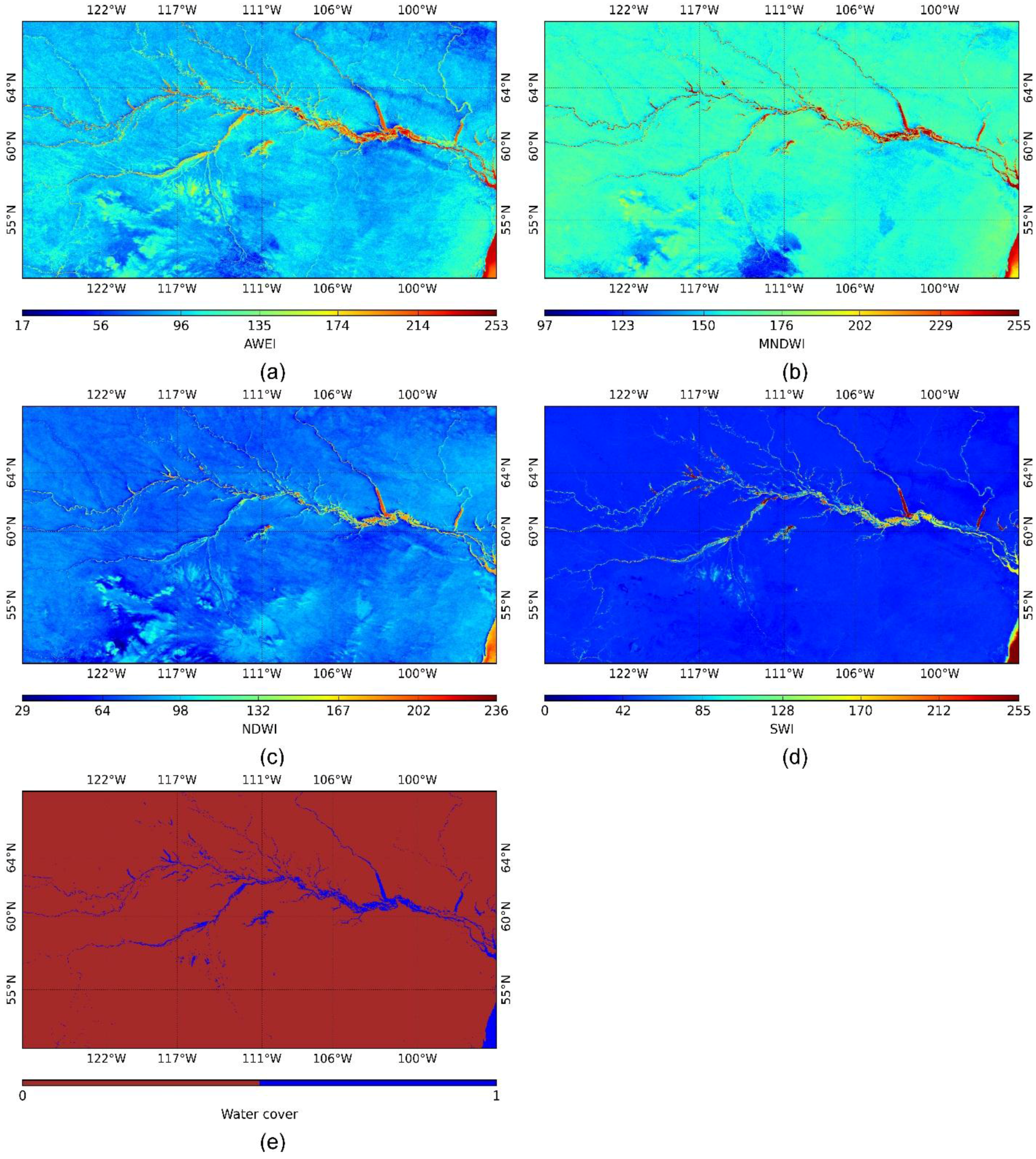
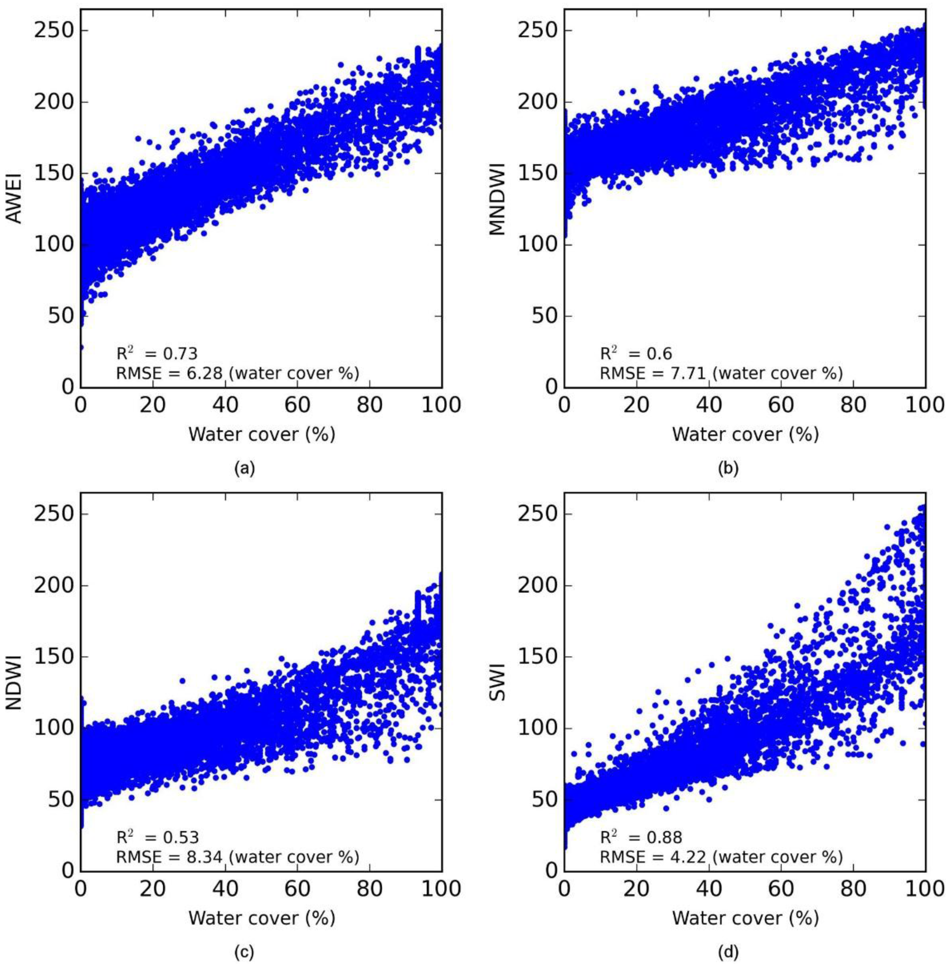
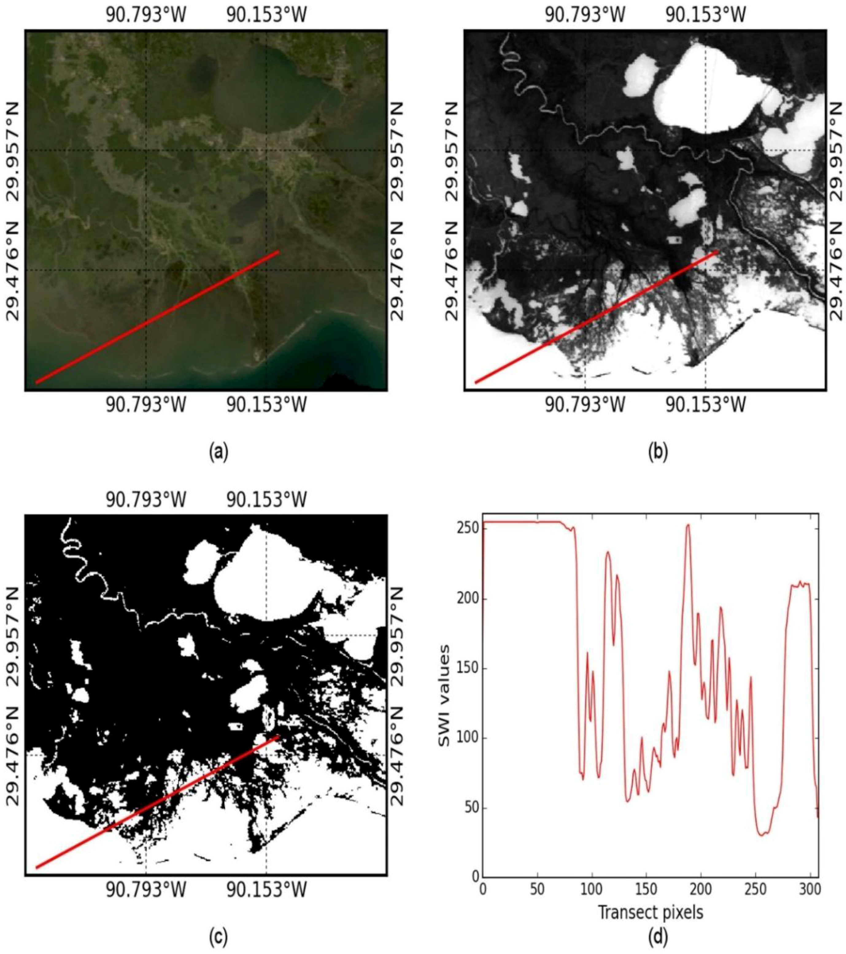
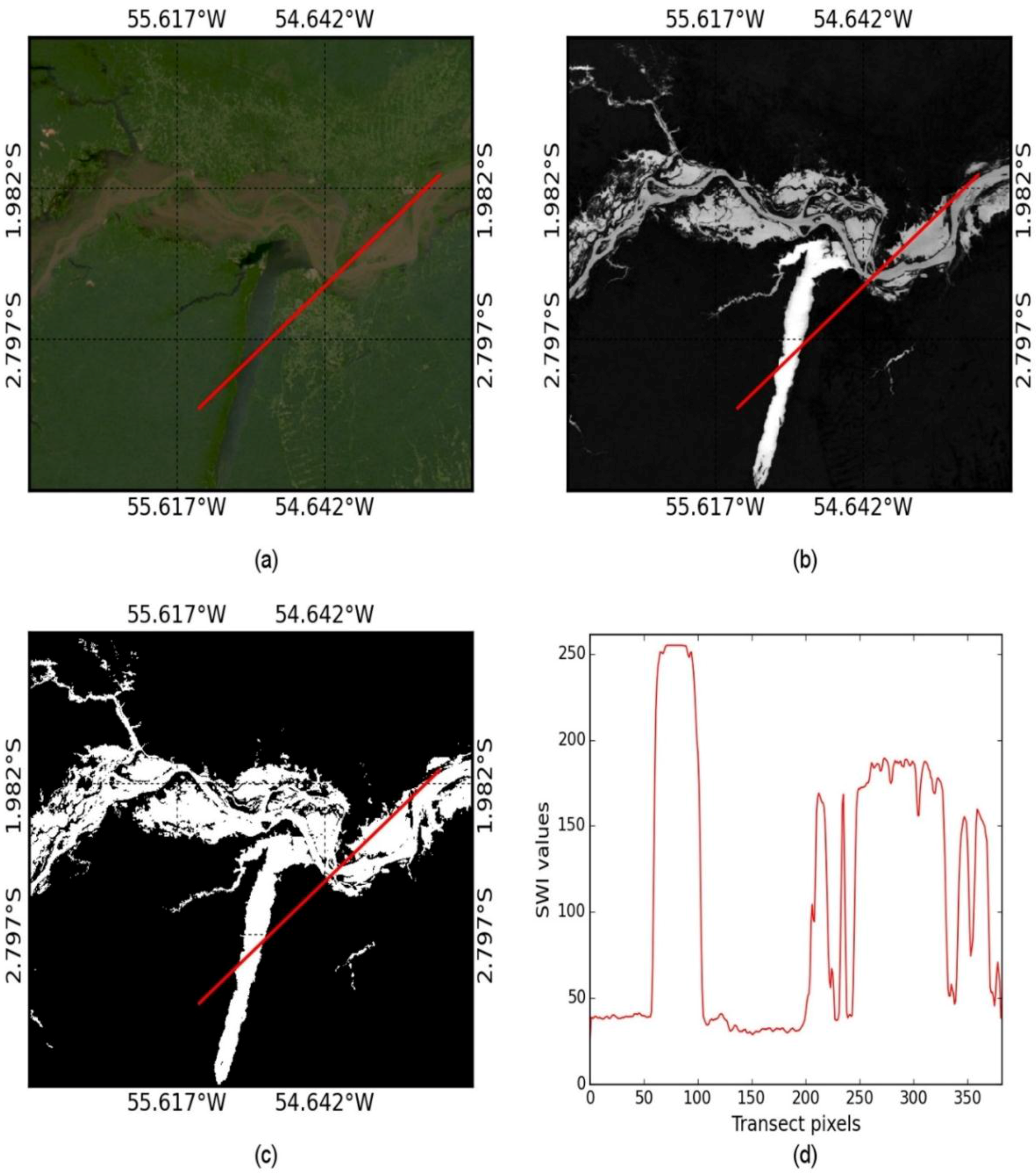
3.3. Performance of SWI in Wet Regions

The reference water map of the wet region is shown in Figure 9 along with four different water index images used.

In the wet region, all the water indices worked well for the estimation of water cover (Figure 10). Nevertheless, the SWI provided the strongest relationship (R² = 0.88, RMSE = 4.22) with the water cover compared to any existing indices. Among the existing indices, the AWEI performed best (R² = 0.73, RMSE = 6.28). This wet region dominated by dense forests is completely free from snow. The short wave infrared based water indices (MNDWI and AWEI) which were not working in snowy and dry regions worked well in this wet region. However, the SWI worked very well in each region in this research.

Figure 9. Plotting of four water indices and water cover map in a wet region: (a) Automated Water Extraction Index (AWEI), (b) Modified Normalized Difference Water Index (MNDWI), (c) Normalized Difference Water Index (NDWI), (d) Superfine Water Index (SWI), (e) Reference water cover map.

Figure 9. Plotting of four water indices and water cover map in a wet region: (a) Automated Water Extraction Index (AWEI), (b) Modified Normalized Difference Water Index (MNDWI), (c) Normalized Difference Water Index (NDWI), (d) Superfine Water Index (SWI), (e) Reference water cover map.

Figure 10. The sensitivity of different water indices to the water cover in a wet region: (a) Automated Water Extraction Index (AWEI) vs. water cover, (b) Modified Normalized Difference Water Index (MNDWI) vs. water cover, (c) Normalized Difference Water Index (NDWI) vs. water cover, (d) Superfine Water Index (SWI) vs. water cover.

Figure 10. The sensitivity of different water indices to the water cover in a wet region: (a) Automated Water Extraction Index (AWEI) vs. water cover, (b) Modified Normalized Difference Water Index (MNDWI) vs. water cover, (c) Normalized Difference Water Index (NDWI) vs. water cover, (d) Superfine Water Index (SWI) vs. water cover.

The monthly variation of the green, near infrared, saturation, and SWI values over the water and non-water areas in a wet region is shown in Figure 11. Due to the presence of dense vegetation, the green reflectance is not very sensitive to the water cover. However, the near infrared reflectance is showing high contrast between the water and non-water areas. Similar to the green reflectance, the saturation from the visible wavelength regions is also not very sensitive to the water cover. However, for water areas, the saturation values are higher than the near infrared reflectance as in the snowy and dry regions. For non-water areas, when the near infrared reflectance is uplifted by introducing the coefficient to it, high contrast with the saturation values was obtained. In this research, the coefficient of 7.0 was used so that the raised near infrared reflectance by this level did not interfere with the saturation values of the water areas everywhere in the globe. Therefore, the SWI has worked very well for discriminating the water areas in all months.

Figure 11. Monthly variation of different parameters over the water and non-water areas in a wet region: (a) Green reflectance, (b) Near infrared reflectance, (c) Saturation values, (d) Superfine Water Index (SWI) values.

Figure 11. Monthly variation of different parameters over the water and non-water areas in a wet region: (a) Green reflectance, (b) Near infrared reflectance, (c) Saturation values, (d) Superfine Water Index (SWI) values.

The true-color composite based saturation values secured very large values compared to the near infrared reflectance in water areas for all the regions under research. For discriminating the water areas from non-water areas, the near infrared reflectance of the non-water areas have to be larger than the saturation values. However, near infrared reflectance of the non-water areas was slightly lower than the saturation values. Therefore, the near infrared reflectance was uplifted by introducing the coefficient to it. Multiplying the near infrared reflectance by the coefficient of 7.0 substantially raised the reflectance of the non-water areas, but slightly increased the reflectance of the water areas because the near infrared reflectance of the water areas was very low. The raised near infrared reflectance of the water areas also did not hit the saturation values of the water areas because the saturation values of the water areas were very large.

The NDWI using the green and near infrared reflectance should discriminate the water areas as long as the green reflectance is larger than the near infrared reflectance for the water areas; and for the non-water areas, the near infrared reflectance is larger than the green reflectance. The green band maintained slightly larger reflectance of the water areas than the near infrared band in dry and wet regions providing the discriminability of the water areas. However, in the snowy region, due to the presence of snow, not only the green reflectance but also the near infrared reflectance of both the water and non-water areas further reduced the discriminability of the NDWI. The partial discrimination in the snowy region by the NDWI was achieved because the near infrared reflectance of the non-water areas was larger than that of the water areas mainly in summer months. Raising the infrared reflectance hits the green reflectance of water areas, and it does not work in case of NDWI. However, the combination of the saturation and uplifted near infrared reflectance provided superior discriminability of the water areas in all the snowy, dry, and wet regions.

Since the SWI measures wetness of the region, when the water bodies are covered by snow it cannot detect the hidden water surface. Therefore, the SWI has discriminated the water areas during summer months only (Figure 5d and Figure 8d). In the snowy region (Figure 5a,b), the higher reflectance of the green and near infrared bands during winter months compared to the summer months are demonstrated very clearly. This is also seen in the dry region (Figure 8a,b) during a few months in winter which there was snow fall but not on the same scale as in the snowy region. However, in the wet region dominated by forests, the winter snowfall is completely absent (Figure 11a,b). Therefore, in the wet region, the SWI discriminated the water surface from the background of non-water surfaces throughout the year (Figure 11d). However, mapping of global water cover is based on the definition of maximum extent of water cover observed in a region avoiding temporary flooding.

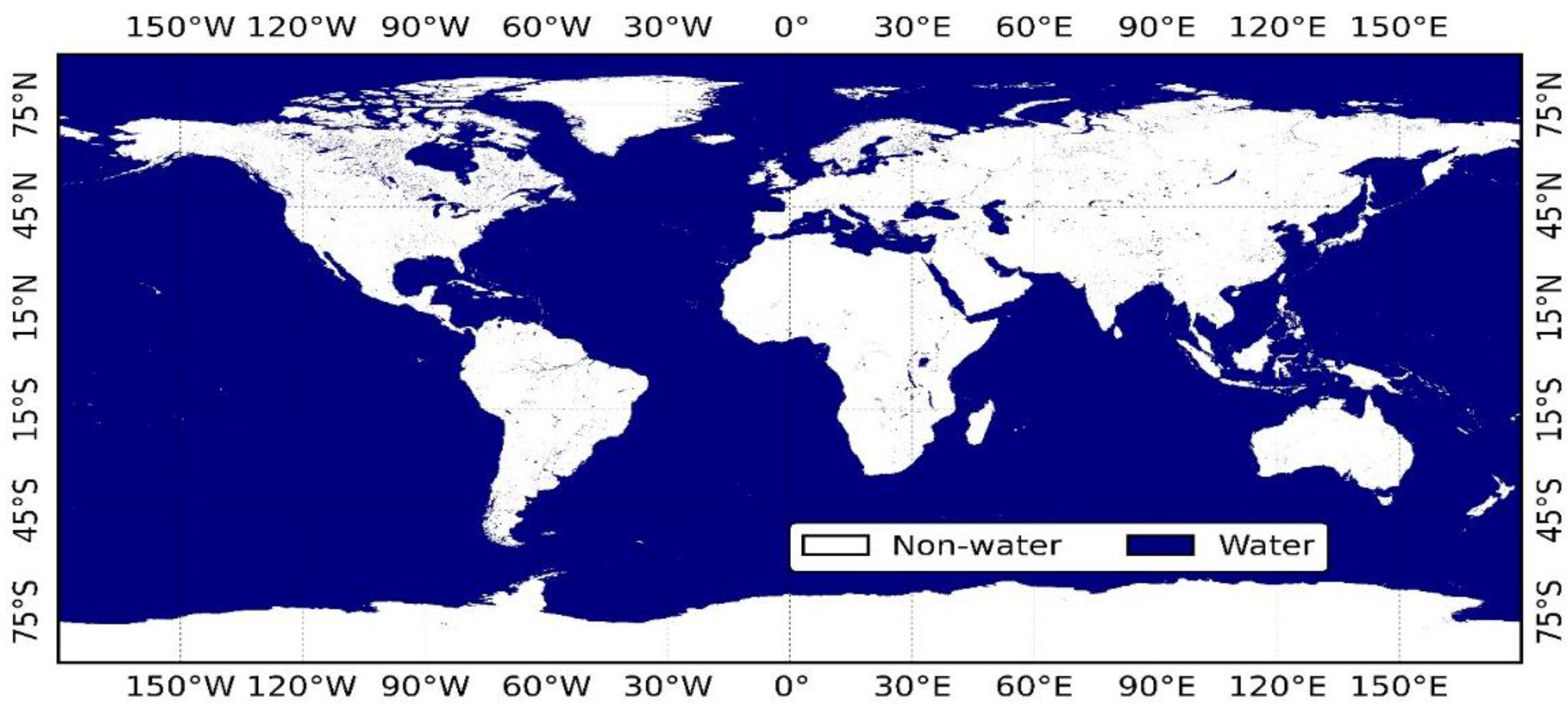
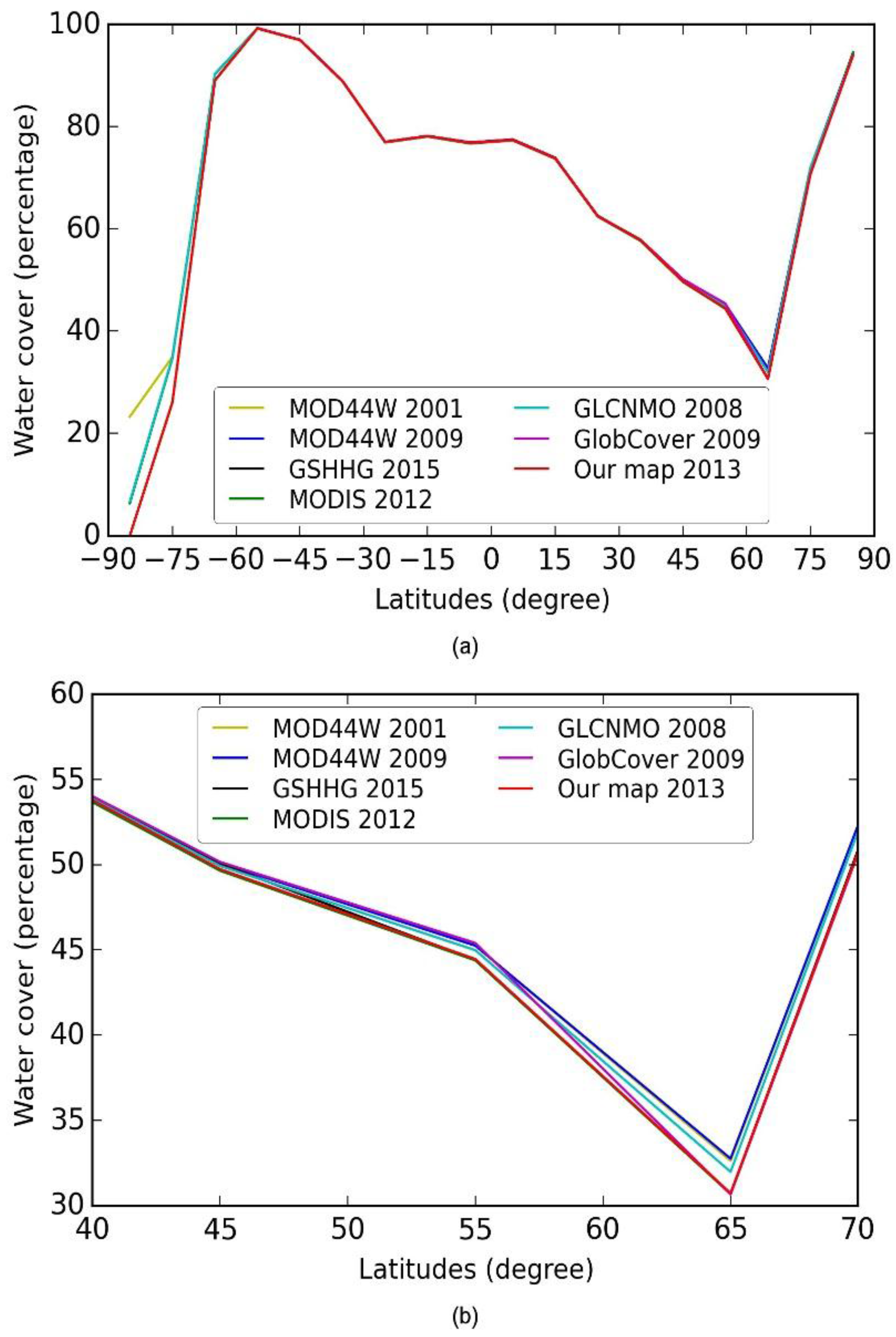
3.4. Performance of the Water Map

The global water cover map of year 2013 produced through the research is shown in Figure 12.

Figure 12. Global water cover map of 2013 produced through the research.

Figure 12. Global water cover map of 2013 produced through the research.

The performance of the SWI based water cover map was examined in a number of places consisting of a variety of background objects and turbidity of water bodies. In spite of a variety of water turbidities as seen in Figure 13a, the SWI successfully discriminated the surface water (Figure 13b) because its values over the turbid water are always higher than the background values (Figure 13d). The extracted water cover in Figure 13c also matches very well with the visually recognized water cover in Figure 13a.

Figure 13. Performance of SWI based extraction of water cover in case of varied turbidity of water bodies: (a) MODIS true-color image, (b) SWI image, (c) Extracted water cover, (d) Profile plot of SWI along the red line drawn.

Figure 13. Performance of SWI based extraction of water cover in case of varied turbidity of water bodies: (a) MODIS true-color image, (b) SWI image, (c) Extracted water cover, (d) Profile plot of SWI along the red line drawn.

In Figure 14, the SWI efficiently detected very narrow water bodies of water as well. The presence of algal bloom in Lake Erie has no effect on the SWI based extraction of the water cover as shown in Figure 15. The aerial proportion of the water seen in the true-color image matches well with the extracted water cover. In case of dark soils and high sediments in Figure 16, the SWI correctly discriminated the surface water, and the extracted water cover is very similar to the water cover existing on the ground. In case of coastal zones with varied shore objects and turbidity as shown in Figure 17, since the SWI provides high contrast between the surface water and non-water areas, the water cover was efficiently extracted and the coastlines were correctly delineated. The MODIS based true-color image in Figure 18 shows the presence of both the turbid and non-turbid water surrounded by dense vegetation. Nevertheless, the SWI efficiently discriminated both types of water, and the extracted cover map is very similar to the photo interpreted water cover. Figure 19 and Figure 20 demonstrate the performance of SWI in case of volcanic areas. Though the SWI values are slightly higher in the active volcanic pixels than in other background pixels, they are far less than the values of the water areas. Therefore, the SWI based cover map worked perfectly, even in the volcanic regions (Figure 19c and Figure 20c). The site-specific case studies conducted in a number of locations confirmed the reliability of the SWI based technique for the extraction and mapping of water cover. The credit for successful extraction and mapping of the water cover in spite of a variety of background objects and turbidity of water goes to SWI. The SWI was designed in such a way that it could broadcast high contrast between the water and non-water areas. Achieving the high contrast is important for the extraction and mapping of water cover because it interacts with a number of complex background objects at a global scale.

Figure 14. Performance of SWI based extraction of water cover in case of narrow water bodies of water bodies: (a) MODIS true-color image, (b) SWI image, (c) Extracted water cover, (d) Profile plot of SWI along the red line drawn.

Figure 14. Performance of SWI based extraction of water cover in case of narrow water bodies of water bodies: (a) MODIS true-color image, (b) SWI image, (c) Extracted water cover, (d) Profile plot of SWI along the red line drawn.

Figure 15. Performance of SWI based extraction of water cover in case of algal bloom: (a) MODIS true-color image, (b) SWI image, (c) Extracted water cover, (d) Profile plot of SWI along the red line drawn.

Figure 15. Performance of SWI based extraction of water cover in case of algal bloom: (a) MODIS true-color image, (b) SWI image, (c) Extracted water cover, (d) Profile plot of SWI along the red line drawn.

Figure 16. Performance of SWI based extraction of water cover in case of dark soils and high sediments: (a) MODIS true-color image, (b) SWI image, (c) Extracted water cover, (d) Profile plot of SWI along the red line drawn.

Figure 16. Performance of SWI based extraction of water cover in case of dark soils and high sediments: (a) MODIS true-color image, (b) SWI image, (c) Extracted water cover, (d) Profile plot of SWI along the red line drawn.

Figure 17. Performance of SWI based extraction of water cover in case of coastal zone with varied shore objects and turbidity: (a) MODIS true-color image, (b) SWI image, (c) Extracted water cover, (d) Profile plot of SWI along the red line drawn.

Figure 17. Performance of SWI based extraction of water cover in case of coastal zone with varied shore objects and turbidity: (a) MODIS true-color image, (b) SWI image, (c) Extracted water cover, (d) Profile plot of SWI along the red line drawn.

Figure 18. Performance of SWI based extraction of water cover in case of dark vegetation with varied turbidity of water bodies: (a) MODIS true-color image, (b) SWI image, (c) Extracted water cover, (d) Profile plot of SWI along the red line drawn.

Figure 18. Performance of SWI based extraction of water cover in case of dark vegetation with varied turbidity of water bodies: (a) MODIS true-color image, (b) SWI image, (c) Extracted water cover, (d) Profile plot of SWI along the red line drawn.

Figure 19. Performance of SWI based extraction of water cover in the case of volcanoes: (a) MODIS true-color image, (b) SWI image, (c) Extracted water cover, (d) Profile plot of SWI along the red line drawn.

Figure 19. Performance of SWI based extraction of water cover in the case of volcanoes: (a) MODIS true-color image, (b) SWI image, (c) Extracted water cover, (d) Profile plot of SWI along the red line drawn.

Figure 20. Performance of SWI based extraction of water cover in the case of volcanoes: (a) MODIS true-color image, (b) SWI image, (c) Extracted water cover, (d) Profile plot of SWI along the red line drawn.

Figure 20. Performance of SWI based extraction of water cover in the case of volcanoes: (a) MODIS true-color image, (b) SWI image, (c) Extracted water cover, (d) Profile plot of SWI along the red line drawn.

The water cover estimated by our water map was compared with the following seven types of existing water maps/products: Global Self-consistent, Hierarchical, High-resolution Geography (GSHHG) database, MODIS land-water mask product (MOD44W, 2001 and 2009), MODIS Land Cover Type Product (MCD12Q1 v5.1, 2012), Global Land Cover by National Mapping Organizations (GLCNMO v2.0, 2008), and European Space Agency’s GlobCover 2009. The percentage water cover estimated by each map was calculated at every 10° interval of latitudes over the whole longitudinal range (−180°–180°). The variation of the water cover with respect to latitudes is plotted in Figure 21. In addition, the percentage of water cover estimated by each map at every interval of 10° latitudes is shown in Table 1.

Figure 21. Variation of percentage water cover with respect to latitudes estimated by seven different maps. The results over the full latitudes in (a) are zoomed in to show details in (b) between 40° and 70° latitudes.

Figure 21. Variation of percentage water cover with respect to latitudes estimated by seven different maps. The results over the full latitudes in (a) are zoomed in to show details in (b) between 40° and 70° latitudes.

The variation of the water cover below −60° latitudes in the Southern hemisphere as distinctly seen in Figure 21a is due to variation of the boundary of Antarctica used by different maps. The boundary of Antarctica estimated by our map matches well with the GSHHG-2015. However, the most important variation of the water cover among the maps are seen between 40° and 70° latitudes. The MOD44W product originally in 250-m resolution is overestimating the water cover in this region compared to all other maps. The GLCNMO-2008 relied on MOD44W-2001 product as the reference data [49] is also overestimating the water cover compared to our map. The details of water bodies as reported by the GLCNMO-2008 and MOD44W-2001/MOD44W-2009 are not seen by 463-m resolution multi-spectral imaging. The difference between MOD44W-2001 and MOD44W-2009 is very minor everywhere in the globe besides Antarctica where MOD44W-2009 is not available. Overall, our map was very similar to the MODIS-2012 everywhere in the globe except in Antarctica. Both the MODIS-2012 and our map-2013 used the MODIS data, and the years they represent are very close to each other.

Table 1. Estimates of percentage water cover by different maps at every interval of 10° latitudes.

Latitudes	Percentage Water Cover Based on Different Maps
	MOD44W 2001	MOD44W 2009	GSHHG 2015	MODIS 2012	GLCNMO 2008	GlobCover 2009	Our map 2013
90°N–80°N	94.36	94.36	94.26	94.52	94.01	93.97	93.86
80°N–70°N	71.91	71.92	71.08	70.83	71.97	70.67	70.81
70°N–60°N	32.62	32.75	30.71	30.68	31.97	30.65	30.72
60°N–50°N	45.25	45.25	44.40	44.38	44.98	45.40	44.46
50°N–40°N	50.10	50.10	50.06	49.64	49.92	50.16	49.73
40°N–30°N	57.86	57.86	57.87	57.68	57.79	57.87	57.84
30°N–20°N	62.52	62.52	62.52	62.41	62.48	62.52	62.48
20°N–10°N	73.83	73.84	73.90	73.72	73.79	73.83	73.78
10°N–00°N	77.42	77.43	77.49	77.31	77.39	77.43	77.36
00°N–10°S	76.89	76.90	76.86	76.70	76.83	76.91	76.81
10°S–20°S	78.14	78.14	78.15	78.05	78.10	78.14	78.16
20°S–30°S	77.01	77.01	76.97	76.91	76.97	77.02	76.97
30°S–40°S	88.92	88.92	88.85	88.85	88.90	88.93	88.91
40°S–50°S	96.95	96.97	96.93	96.92	96.95	96.96	96.93
50°S–60°S	99.23	99.24	99.23	99.21	99.23	99.26	99.21
60°S–70°S	90.33	NA	89.05	90.25	90.31	NA	89.01
70°S–80°S	34.96	NA	26.07	34.69	34.89	NA	26.08
80°S–90°S	23.28	NA	0.00	6.34	6.69	NA	0.00

Table 1. Estimates of percentage water cover by different maps at every interval of 10° latitudes.

Latitudes	Percentage Water Cover Based on Different Maps
	MOD44W 2001	MOD44W 2009	GSHHG 2015	MODIS 2012	GLCNMO 2008	GlobCover 2009	Our map 2013
90°N–80°N	94.36	94.36	94.26	94.52	94.01	93.97	93.86
80°N–70°N	71.91	71.92	71.08	70.83	71.97	70.67	70.81
70°N–60°N	32.62	32.75	30.71	30.68	31.97	30.65	30.72
60°N–50°N	45.25	45.25	44.40	44.38	44.98	45.40	44.46
50°N–40°N	50.10	50.10	50.06	49.64	49.92	50.16	49.73
40°N–30°N	57.86	57.86	57.87	57.68	57.79	57.87	57.84
30°N–20°N	62.52	62.52	62.52	62.41	62.48	62.52	62.48
20°N–10°N	73.83	73.84	73.90	73.72	73.79	73.83	73.78
10°N–00°N	77.42	77.43	77.49	77.31	77.39	77.43	77.36
00°N–10°S	76.89	76.90	76.86	76.70	76.83	76.91	76.81
10°S–20°S	78.14	78.14	78.15	78.05	78.10	78.14	78.16
20°S–30°S	77.01	77.01	76.97	76.91	76.97	77.02	76.97
30°S–40°S	88.92	88.92	88.85	88.85	88.90	88.93	88.91
40°S–50°S	96.95	96.97	96.93	96.92	96.95	96.96	96.93
50°S–60°S	99.23	99.24	99.23	99.21	99.23	99.26	99.21
60°S–70°S	90.33	NA	89.05	90.25	90.31	NA	89.01
70°S–80°S	34.96	NA	26.07	34.69	34.89	NA	26.08
80°S–90°S	23.28	NA	0.00	6.34	6.69	NA	0.00

Table 2 shows the confusion matrix computed between the photo-interpretation based validation data and water cover map produced in this research. The overall accuracy of our water cover map was calculated to be 92.84%.

Table 2. Confusion matrix of the global water map produced in this research.

Predicted	Photo-Interpretation		Accuracy
	Water (12,500 points)	Non-water (12,500 points)
Water	10,867	157	98.57% (User)
Non-water	1633	12,343	88.31% (User)
Accuracy	86.93% (Producer)	98.74% (Producer)	92.84% (Overall)

Table 2. Confusion matrix of the global water map produced in this research.

Predicted	Photo-Interpretation		Accuracy
	Water (12,500 points)	Non-water (12,500 points)
Water	10,867	157	98.57% (User)
Non-water	1633	12,343	88.31% (User)
Accuracy	86.93% (Producer)	98.74% (Producer)	92.84% (Overall)

4. Conclusions

The breakthrough of the true-color composite based saturation is that it secured very large values compared to the near infrared reflectance in water areas. The normalized difference between the saturation values and the uplifted near infrared reflectance provided a standard measurement of the wetness of the surface with the dynamic range of −1 to 1. The resulted water index called Superfine Water Index (SWI) captured finer details of the surface water in most of the months for all land surface types in the research. The use of 90-percentile SWI values for the extraction and mapping of the water cover assured much higher contrast of the water pixels from any backgrounds despite that MODIS data cannot discriminate the water areas in every month in snowy regions.

The performance of the water indices strongly varied with the type of land surface. In the snowy region dominated by winter snow falls, only the NDWI and SWI worked, explaining 58% and 95% variation of the water cover, respectively. The AWEI and MNDWI using the shortwave infrared reflectance failed to capture the variation of water cover there. In the dry region dominated by bare soil and permanent snow, though the AWEI and MNDWI performed better in the snowy region, only the NDWI and SWI worked satisfactorily, explaining 81% and 97% variation of the water cover, respectively. All the indices worked well in the case of the wet region dominated by dense forest. However, SWI and AWEI worked most effectively, by explaining 88% and 73% variation of the water cover, respectively. The sensitivity analysis of the water indices to the water cover in the major types of land surface in the research proved the supremacy of the newly developed SWI because it was most sensitive to the water cover compared to any existing water indices. The analysis of monthly variations of the SWI showed that the SWI could efficiently discriminate the water areas in most months in the snowy and dry regions, and in all months in the wet region. Moreover, the SWI provided high contrast between the water and non-water pixels. Achievement of this high contrast greatly influences the success of the water index for extracting the water cover, because the water bodies are usually mixed with complex types of background objects. The sensitivity of the SWI was recursively tested in different land surfaces and was found to be the best measure of surface water cover.

Since the SWI measures the wetness of a surface, it should be capable of detecting the surface water changes by weather patterns like El Niño and La Niña, extreme weather events such as flooding, and phenology of the water bodies. However, in this research, the potential of the SWI was assessed for extraction and mapping of the marine and continental surface water at a global scale. We worked according to the definition of annual maximum extent of surface water avoiding temporary flooding. Since the inland water bodies with diverse water levels and turbidity surrounded by complex mixtures of land cover types are very different to the ocean water and shore objects, training data from both the ocean water and inland water bodies were supplied for extracting and mapping the water cover at a global scale.

A brand new map of global water cover of the year 2013 was produced by designing a new methodology. The overall accuracy of 92.84% of our water cover map confirmed the reliability of the methodology developed in this research. The reference library constructed in this research can run the overall mapping procedure automatically. However, the global water cover map produced using the SWI did not differ significantly to the existing water maps. The water cover estimated by this research matched very well with the estimates by MODIS-2012 in most of the geographical regions. None of the existing maps were created by using water indices. The MODIS Land cover type product used supervised classification (decision trees) approach for classifying the water areas. It was based on 135 feature images as the inputs created from monthly composites of MODIS seven bands, land surface temperature (LST), enhanced vegetation index (EVI), and their annual metrics (minimum, maximum and mean values); and supported by training data from 1860 sites distributed across the Earth’s land areas [48]. The water cover was not mapped separately in the case of this research. Since different mapping approaches and methodologies were used by each of the existing maps and they were produced by using composite data of multiple years, the water cover estimations by them are not directly comparable. Moreover, reproducing the water cover map for the year 2013 by exactly following their techniques and comparing with the new results is also not feasible due to many reasons. Therefore, the comparison results shown in Figure 21 and Table 1 are for reference purposes only to show how the estimates differ to each other. The similarity of our map using new methodology for the MODIS-2012 map based on a supervised classification approach means that the new mapping methodology works well. We expect that this methodology can contribute to seasonal and annual change analysis of water cover at a global scale.

References

1. Ouma, Y.O.; Tateishi, R. A water index for rapid mapping of shoreline changes of five east African rift valley lakes: An empirical analysis using Landsat TM and ETM+ data. Int. J. Remote Sens. 2006, 27, 3153–3181. [Google Scholar] [CrossRef]
2. Alesheikh, A.A.; Ghorbanali, A.; Nouri, N. Coastline change detection using remote sensing. Int. J. Environ. Sci. Technol. 2007, 4, 61–66. [Google Scholar] [CrossRef]
3. Sesli, F.; Karsli, F.; Colkesen, I.; Akyol, N. Monitoring the changing position of coastlines using aerial and satellite image data: An example from the eastern coast of Trabzon, Turkey. Environ. Monit. Assess. 2009, 153, 391–403. [Google Scholar] [CrossRef] [PubMed]
4. Pardo-Pascual, J.E.; Almonacid-Caballer, J.; Ruiz, L.A.; Palomar-Vázquez, J. Automatic extraction of shorelines from Landsat TM and ETM+ multi-temporal images with subpixel precision. Remote Sens. Environ. 2012, 123, 1–11. [Google Scholar] [CrossRef]
5. Mujabar, P.S.; Chandrasekar, N. Shoreline change analysis along the coast between Kanyakumari and Tuticorin of India using remote sensing and GIS. Arab. J. Geosci. 2013, 6, 647–664. [Google Scholar] [CrossRef]
6. Jiang, H.; Feng, M.; Zhu, Y.; Lu, N.; Huang, J.; Xiao, T. An automated method for extracting rivers and lakes from Landsat imagery. Remote Sens. 2014, 6, 5067–5089. [Google Scholar] [CrossRef]
7. Tran Thi, V.; Tien Thi Xuan, A.; Phan Nguyen, H.; Dahdouh-Guebas, F.; Koedam, N. Application of remote sensing and GIS for detection of long-term mangrove shoreline changes in Mui Ca Mau, Vietnam. Biogeosciences 2014, 11, 3781–3795. [Google Scholar] [CrossRef]
8. Klein, I.; Dietz, A.; Gessner, U.; Dech, S.; Kuenzer, C. Results of the Global WaterPack: A novel product to assess inland water body dynamics on a daily basis. Remote Sens. Lett. 2015, 6, 78–87. [Google Scholar] [CrossRef]
9. Klein, I.; Dietz, A.J.; Gessner, U.; Galayeva, A.; Myrzakhmetov, A.; Kuenzer, C. Evaluation of seasonal water body extents in Central Asia over the past 27 years derived from medium-resolution remote sensing data. Int. J. Appl. Earth Observ. Geoinform. 2014, 26, 335–349. [Google Scholar] [CrossRef]
10. Ghosh, M.K.; Kumar, L.; Roy, C. Monitoring the coastline change of Hatiya island in Bangladesh using remote sensing techniques. ISPRS J. Photogramm. Remote Sens. 2015, 101, 137–144. [Google Scholar] [CrossRef]
11. García-Rubio, G.; Huntley, D.; Russell, P. Evaluating shoreline identification using optical satellite images. Mar. Geol. 2015, 359, 96–105. [Google Scholar] [CrossRef]
12. Shetty, A.; Jayappa, K.S.; Mitra, D. Shoreline change analysis of Mangalore coast and morphometric analysis of Netravathi-Gurupur and Mulky-Pavanje spits. Aquat. Proced. 2015, 4, 182–189. [Google Scholar] [CrossRef]
13. Rokni, K.; Ahmad, A.; Solaimani, K.; Hazini, S. A new approach for surface water change detection: Integration of pixel level image fusion and image classification techniques. Int. J. Appl. Earth Observ. Geoinform. 2015, 34, 226–234. [Google Scholar] [CrossRef]
14. Baghdadi, N.; Pedreros, R.; Lenotre, N.; Dewez, T.; Paganini, M. Impact of polarization and incidence of the ASAR sensor on coastline mapping: Example of Gabon. Int. J. Remote Sens. 2007, 28, 3841–3849. [Google Scholar] [CrossRef]
15. Lewis, M.; Schumann, G.; Bates, P.; Horsburgh, K. Understanding the variability of an extreme storm tide along a coastline. Estuar. Coast. Shelf Sci. 2013, 123, 19–25. [Google Scholar] [CrossRef]
16. Westerhoff, R.S.; Kleuskens, M.P.H.; Winsemius, H.C.; Huizinga, H.J.; Brakenridge, G.R.; Bishop, C. Automated global water mapping based on wide-swath orbital synthetic-aperture radar. Hydrol. Earth Syst. Sci. 2013, 17, 651–663. [Google Scholar] [CrossRef]
17. Nunziata, F.; Migliaccio, M.; Xiaofeng, L.; Xianwen, D. Coastline extraction using dual-polarimetric COSMO-Skymed PingPong mode SAR data. IEEE Geosci. Remote Sens. Lett. 2014, 11, 104–108. [Google Scholar] [CrossRef]
18. Li, X.; Damen, M.C.J. Coastline change detection with satellite remote sensing for environmental management of the Pearl River Estuary, China. J. Marine Syst. 2010, 82, S54–S61. [Google Scholar] [CrossRef]
19. Eugenio, F.; Marcello, J.; Martin, J. High-resolution maps of bathymetry and benthic habitats in shallow-water environments using multispectral remote sensing imagery. IEEE Trans. Geosci. Remote Sens. 2015, 53, 3539–3549. [Google Scholar] [CrossRef]
20. Kroon, A.; Davidson, M.A.; Aarninkhof, S.G.J.; Archetti, R.; Armaroli, C.; Gonzalez, M.; Medri, S.; Osorio, A.; Aagaard, T.; Holman, R.A.; et al. Application of remote sensing video systems to coastline management problems. Coast. Eng. 2007, 54, 493–505. [Google Scholar] [CrossRef]
21. Van Koningsveld, M.; Davidson, M.; Huntley, D.; Medina, R.; Aarninkhof, S.; Jiménez, J.A.; Ridgewell, J.; de Kruif, A. A critical review of the CoastView project: Recent and future developments in coastal management video systems. Coast. Eng. 2007, 54, 567–576. [Google Scholar] [CrossRef]
22. Davidson, M.; Van Koningsveld, M.; de Kruif, A.; Rawson, J.; Holman, R.; Lamberti, A.; Medina, R.; Kroon, A.; Aarninkhof, S. The coastview project: Developing video-derived coastal state indicators in support of coastal zone management. Coast. Eng. 2007, 54, 463–475. [Google Scholar] [CrossRef]
23. Pianca, C.; Holman, R.; Siegle, E. Shoreline variability from days to decades: Results of long-term video imaging. J. Geophys. Res.: Ocean. 2015, 120, 2159–2178. [Google Scholar] [CrossRef]
24. Irish, J.L.; White, T.E. Coastal engineering applications of high-resolution Lidar bathymetry. Coast. Eng. 1998, 35, 47–71. [Google Scholar] [CrossRef]
25. Sallenger, A.H., Jr.; Krabill, W.B.; Swift, R.N.; Brock, J.; List, J.; Hansen, M.; Holman, R.A.; Manizade, S.; Sontag, J.; Meredith, A. Evaluation of airborne topographic Lidar for quantifying beach changes. J. Coast. Res. 2003, 19, 125–133. [Google Scholar]
26. Brock, J.C.; Purkis, S.J. The emerging role of lidar remote sensing in coastal research and resource management. J. Coast. Res. 2009. [Google Scholar] [CrossRef]
27. Gens, R. Remote sensing of coastlines: Detection, extraction and monitoring. Int. J. Remote Sens. 2010, 31, 1819–1836. [Google Scholar] [CrossRef]
28. Liu, H.; Jezek, K.C. Automated extraction of coastline from satellite imagery by integrating canny edge detection and locally adaptive thresholding methods. Int. J. Remote Sens. 2004, 25, 937–958. [Google Scholar] [CrossRef]
29. Zhang, T.; Yang, X.; Hu, S.; Su, F. Extraction of coastline in aquaculture coast from multispectral remote sensing images: Object-based region growing integrating edge detection. Remote Sens. 2013, 5, 4470–4487. [Google Scholar] [CrossRef]
30. Pekel, J.F.; Vancutsem, C.; Bastin, L.; Clerici, M.; Vanbogaert, E.; Bartholomé, E.; Defourny, P. A near real-time water surface detection method based on HSV transformation of MODIS multi-spectral time series data. Remote Sens. Environ. 2014, 140, 704–716. [Google Scholar] [CrossRef]
31. Smith, A.R. Color gamut transform pairs. ACM Siggraph Computer Graph. 1978, 12, 12–19. [Google Scholar] [CrossRef]
32. Chan, T.F.; Kang, S.H.; Shen, J. Total variation denoising and enhancement of color images based on the CB and HSV color models. J. Vis. Commun. Image Represent. 2001, 12, 422–435. [Google Scholar] [CrossRef]
33. Verpoorter, C.; Kutser, T.; Seekell, D.A.; Tranvik, L.J. A global inventory of lakes based on high-resolution satellite imagery. Geophys. Res. Lett. 2014, 41, 6396–6402. [Google Scholar] [CrossRef]
34. Feng, M.; Sexton, J.O.; Channan, S.; Townshend, J.R. A global, high-resolution (30-m) inland water body dataset for 2000: First results of a topographic-spectral classification algorithm. Int. J. Digit. Earth 2015. [Google Scholar] [CrossRef]
35. McFeeters, S.K. The use of the Normalized Difference Water Index (NDWI) in the delineation of open water features. Int. J. Remote Sens. 1996, 17, 1425–1432. [Google Scholar] [CrossRef]
36. Lu, S.; Wu, B.; Yan, N.; Wang, H. Water body mapping method with HJ-1A/B satellite imagery. Int. J. Appl. Earth Observ. Geoinform. 2011, 13, 428–434. [Google Scholar] [CrossRef]
37. Feng, L.; Hu, C.; Chen, X.; Cai, X.; Tian, L.; Gan, W. Assessment of inundation changes of Poyang lake using MODIS observations between 2000 and 2010. Remote Sens. Environ. 2012, 121, 80–92. [Google Scholar] [CrossRef]
38. Rango, A.; Salomonson, V.V. Regional flood mapping from space. Water Resour. Res. 1974, 10, 473–484. [Google Scholar] [CrossRef]
39. Huang, C.; Chen, Y.; Wu, J. Mapping spatio-temporal flood inundation dynamics at large river basin scale using time-series flow data and MODIS imagery. Int. J. Appl. Earth Observ. Geoinform. 2014, 26, 350–362. [Google Scholar] [CrossRef]
40. Gao, B.-C. NDWI—A normalized difference water index for remote sensing of vegetation liquid water from space. Remote Sens. Environ. 1996, 58, 257–266. [Google Scholar] [CrossRef]
41. Jackson, T.J.; Chen, D.; Cosh, M.; Li, F.; Anderson, M.; Walthall, C.; Doriaswamy, P.; Hunt, E.R. Vegetation water content mapping using Landsat data derived normalized difference water index for corn and soybeans. Remote Sens. Environ. 2004, 92, 475–482. [Google Scholar] [CrossRef]
42. Xu, H. Modification of normalised difference water index (NDWI) to enhance open water features in remotely sensed imagery. Int. J. Remote Sens. 2006, 27, 3025–3033. [Google Scholar] [CrossRef]
43. Feyisa, G.L.; Meilby, H.; Fensholt, R.; Proud, S.R. Automated water extraction index: A new technique for surface water mapping using Landsat imagery. Remote Sens. Environ. 2014, 140, 23–35. [Google Scholar] [CrossRef]
44. Ayana, E.K.; Philpot, W.D.; Melesse, A.M.; Steenhuis, T.S. Assessing the potential of MODIS/Terra version 5 images to improve near shore lake bathymetric surveys. Int. J. Applied Earth Observ. Geoinform. 2015, 36, 13–21. [Google Scholar] [CrossRef]
45. Wessel, P.; Smith, W.H.F. A global, self-consistent, hierarchical, high-resolution shoreline database. J. Geophys. Res.: Solid Earth 1996, 101, 8741–8743. [Google Scholar] [CrossRef]
46. Salomon, J.; Hodges, J.; Friedl, M.; Schaaf, C.; Strahler, A.; Gao, F.; Schneider, A.; Zhang, X.; El Saleous, N.; Wolfe, R.E. Global land water mask derived from MODIS Nadir BRDF-adjusted reflectances (NBAR) and the MODIS land cover algorithm. In IEEE Geoscience and Remote Sensing Symposium, Alaska, AK, USA, 20–24 September 2004.
47. Carroll, M.L.; Townshend, J.R.; DiMiceli, C.M.; Noojipady, P.; Sohlberg, R.A. A new global raster water mask at 250 m resolution. Int. J. Digit. Earth 2009, 2, 291–308. [Google Scholar] [CrossRef]
48. Friedl, M.A.; Sulla-Menashe, D.; Tan, B.; Schneider, A.; Ramankutty, N.; Sibley, A.; Huang, X. Modis collection 5 global land cover: Algorithm refinements and characterization of new datasets. Remote Sens. Environ. 2010, 114, 168–182. [Google Scholar] [CrossRef]
49. Tateishi, R.; Hoan, N.T.; Kobayashi, T.; Alsaaideh, B.; Tana, G.; Phong, D.X. Production of global land cover data–GLCNMO2008. J. Geogr. Geol. 2014, 6, 99–122. [Google Scholar] [CrossRef]
50. Arino, O.; Ramos Perez, J.J.; Kalogirou, V.; Bontemps, S.; Defourny, P.; Van Bogaert, E. Global land cover map for 2009 (GlobCover 2009). ESA & UCL 2012. [Google Scholar] [CrossRef]
51. Gorny, A.J. World Data Bank II General User GuideRep; Central Intelligence Agency: Washington, DC, USA, 1977. [Google Scholar]
52. Soluri, E.; Woodson, V. Le fichier WVS (World Vector Shoreline). Rev. Hydrogr. Int. 1990, 67, 27–36. [Google Scholar]
53. Loveland, T.R.; Belward, A.S. The IGBP-DIS global 1km land cover data set, DISCover: First results. Int. J. Remote Sens. 1997, 18, 3289–3295. [Google Scholar] [CrossRef]
54. Lobser, S.E.; Cohen, W.B. MODIS tasselled cap: Land cover characteristics expressed through transformed MODIS data. Int. J. Remote Sens. 2007, 28, 5079–5101. [Google Scholar] [CrossRef]
55. Schaaf, C.B.; Gao, F.; Strahler, A.H.; Lucht, W.; Li, X.; Tsang, T.; Strugnell, N.C.; Zhang, X.; Jin, Y.; Muller, J.-P.; et al. First operational BRDF, albedo nadir reflectance products from MODIS. Remote Sens. Environ. 2002, 83, 135–148. [Google Scholar] [CrossRef]
56. Hu, B.; Lucht, W.; Li, X.; Strahler, A.H. Validation of kernel-driven semiempirical models for the surface bidirectional reflectance distribution function of land surfaces. Remote Sens. Environ. 1997, 62, 201–214. [Google Scholar] [CrossRef]
57. Liang, S.; Fang, H.; Chen, M.; Shuey, C.J.; Walthall, C.; Daughtry, C.; Morisette, J.; Schaaf, C.; Strahler, A. Validating MODIS land surface reflectance and albedo products: Methods and preliminary results. Remote Sens. Environ. 2002, 83, 149–162. [Google Scholar] [CrossRef]
58. Disney, M.; Lewis, P.; Thackrah, G.; Quaife, T.; Barnsley, M. Comparison of MODIS broadband albedo over an agricultural site with ground measurements and values derived from earth observation data at a range of spatial scales. Int. J. Remote Sens. 2004, 25, 5297–5317. [Google Scholar] [CrossRef]
59. Salomon, J.G.; Schaaf, C.B.; Strahler, A.H.; Feng, G.; Yufang, J. Validation of the MODIS bidirectional reflectance distribution function and albedo retrievals using combined observations from the aqua and terra platforms. IEEE Trans. Geosci. Remote Sens. 2006, 44, 1555–1565. [Google Scholar] [CrossRef]
60. Román, M.O.; Schaaf, C.B.; Woodcock, C.E.; Strahler, A.H.; Yang, X.; Braswell, R.H.; Curtis, P.S.; Davis, K.J.; Dragoni, D.; Goulden, M.L.; et al. The MODIS (Collection V005) BRDF/albedo product: Assessment of spatial representativeness over forested landscapes. Remote Sens. Environ. 2009, 113, 2476–2498. [Google Scholar]
61. Sharma, R.C.; Kajiwara, K.; Honda, Y. Estimation of forest canopy structural parameters using kernel-driven bi-directional reflectance model based multi-angular vegetation indices. ISPRS J. Photogramm. Remote Sens. 2013, 78, 50–57. [Google Scholar] [CrossRef]
62. Pajak, M.J.; Leatherman, S. The high water line as shoreline indicator. J. Coast. Res. 2002, 18, 329–337. [Google Scholar]
63. Stockdonf, H.F.; Sallenger, A.H., Jr.; List, J.H.; Holman, R.A. Estimation of shoreline position and change using airborne topographic Lidar data. J. Coast. Res. 2002, 18, 502–513. [Google Scholar]
64. Grady, L. Random walks for image segmentation. IEEE Trans. Pattern Anal. Mach. Intell. 2006, 28, 1768–1783. [Google Scholar] [CrossRef] [PubMed]