
Hyperspectral Differentiation of Phytoplankton Taxonomic Groups: A Comparison between Using Remote Sensing Reflectance and Absorption Spectra


Abstract
:
1. Introduction
2. Data and Methods
2.1. Algal Cultures
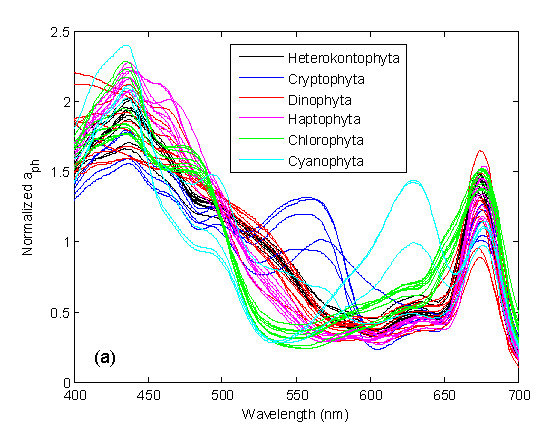
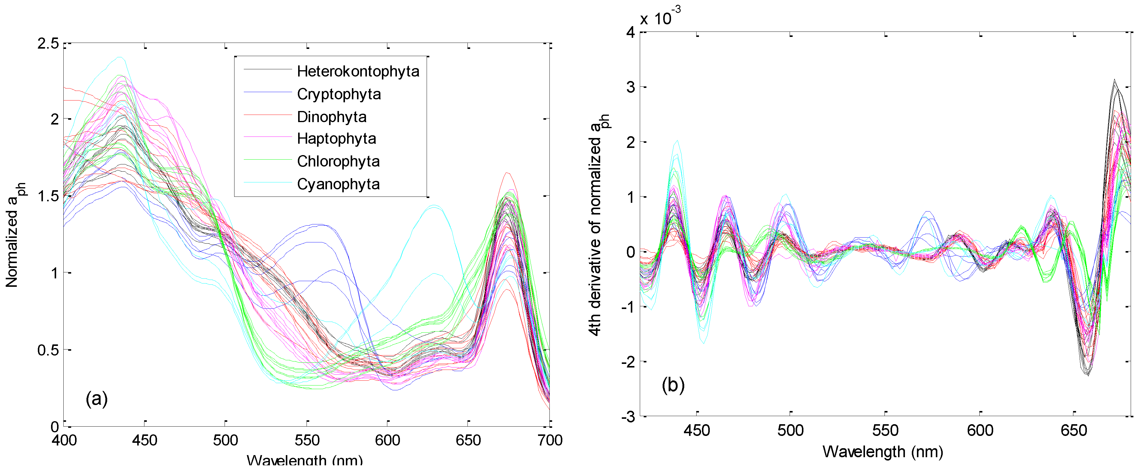
2.2. Absorption Measurements and Normalization
2.3. HydroLight Simulations of Hyperspectral Remote Sensing Reflectance
- Phytoplankton absorption: eight chlorophyll concentrations (Chl) were set for each measured varying from 0.1 to 100 mg∙m−3 (0.1, 0.5, 1, 3, 5, 10, 50, and 100 mg∙m−3). To determine aph(λ) for these different Chl concentrations, we used the empirical relationship by Bricaud et al. [51] to calculate aph(440): aph(440) = 0.0654 [Chl]0.728. The modeled absorption spectra were obtained by multiplying the normalized absorption spectra with aph(440), i.e., . In the end, eight sets of were obtained for these different Chl concentrations.
- Chromophoric dissolved organic matter (CDOM) absorption: the HydroLight default exponential model for CDOM absorption with fixed values at 440 nm, aCDOM(440) (m−1), and a single spectral slope of 0.014 nm−1 was used [52]: . In the simulations two CDOM concentrations were used with aCDOM(440) = 0.0 and 0.1 m−1 to check how the varying CDOM concentrations do influence the performance of the differentiation.
- Absorption by non-algal particles, aNAP(λ) (m−1), was determined using a mass-specific absorption coefficients due to non-algal particles, aNAP*(λ) (m2∙mg−1), and a particle mass concentration, which is often referred to as total suspended matter concentrations (TSM), i.e., . The spectral shape of the aNAP* used is very similar to the HydroLight standard (average coefficient), but is based on spectrally exponentially-shaped in situ measurements from the Baltic Sea and Elbe River (unpublished data). Two TSM values were set for different simulation scenarios (TSM = 0 and 1 g∙m−3).
2.4. Inversion of Absorption Spectra from Simulated Rrs(λ)
2.5. Derivative Analysis
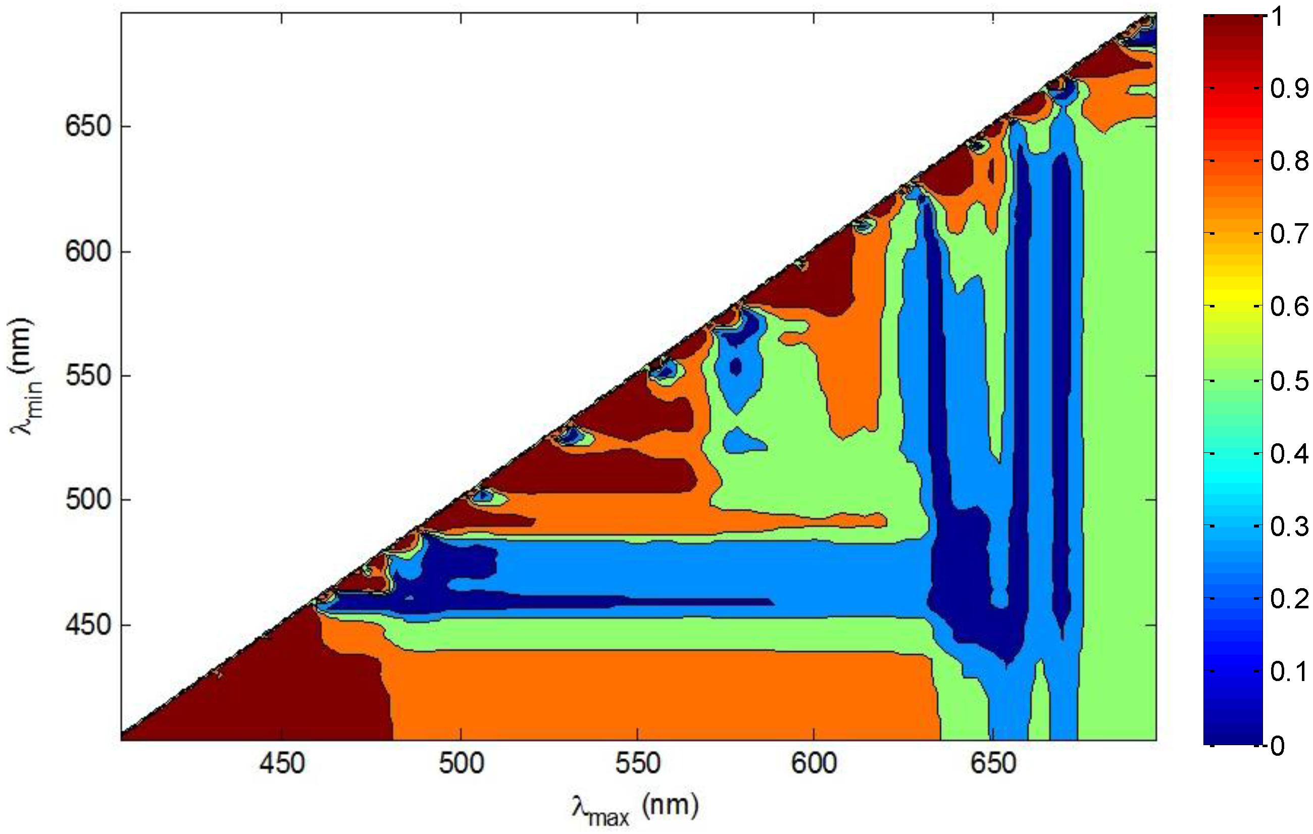
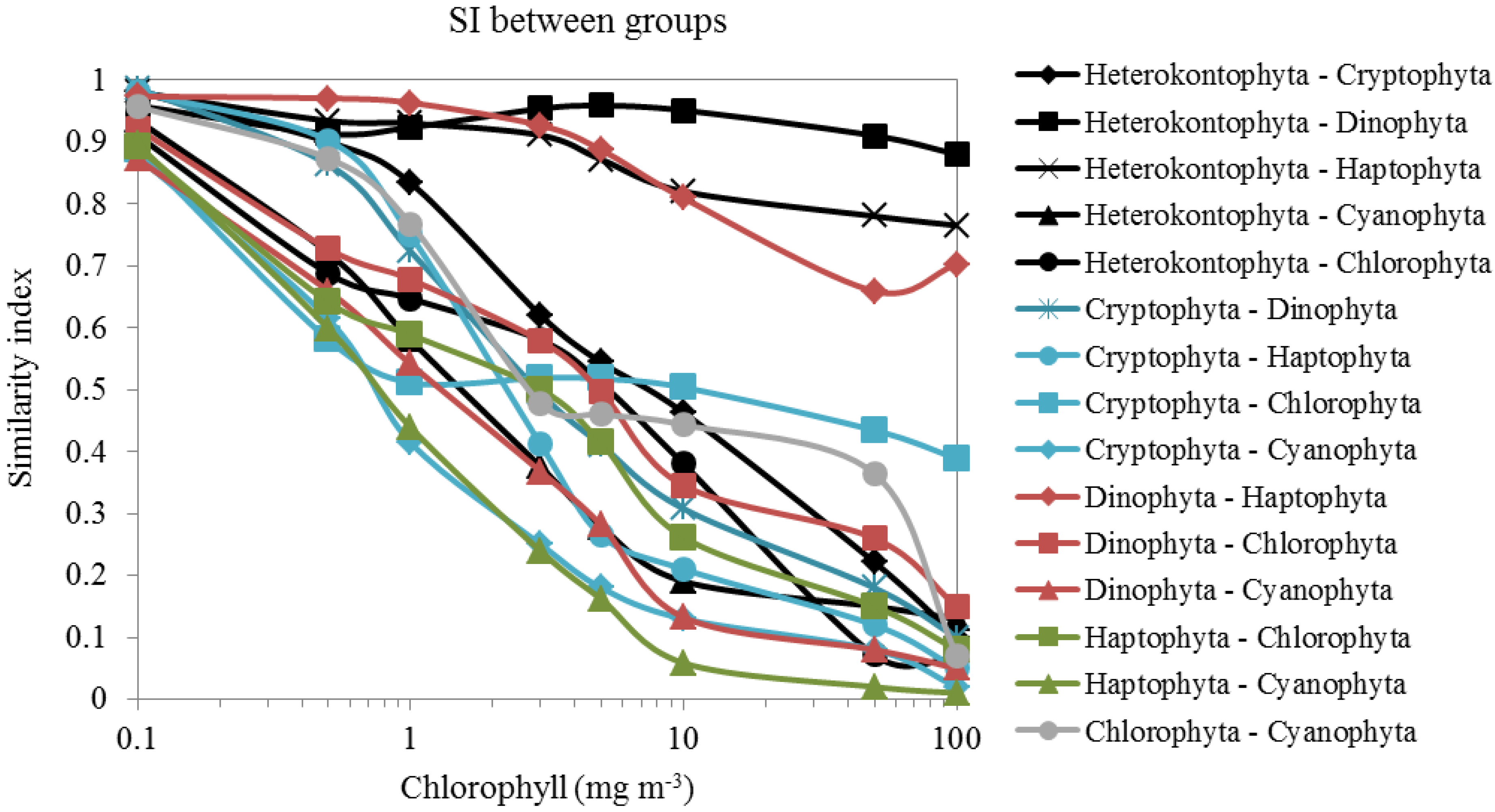
2.6. Similarity Index (SI) and Clustering Analysis
3. Results
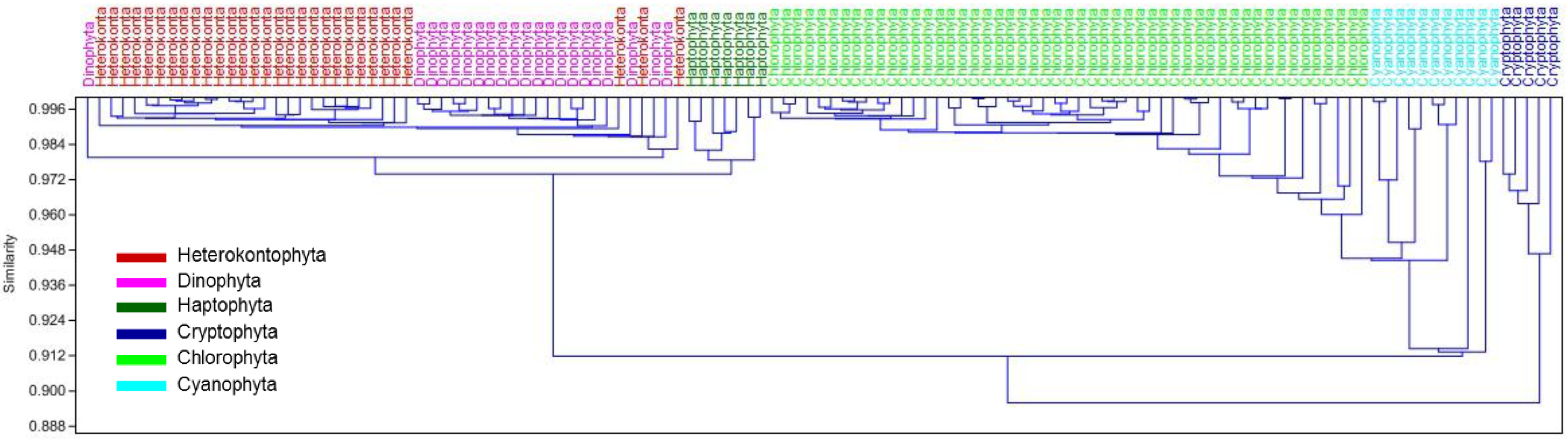
3.1. Derivative Analysis and Clustering of Algal Absorption Spectra


| Heterokontophyta | Dinophyta | Haptophyta | Cryptophyta | Chlorophyta | Cyanobacteria | |
|---|---|---|---|---|---|---|
| Measured aph(λ) | 27/30 | 20/21 | 7/7 | 5/5 | 51/51 | 11/11 |
| Simulated Rrs(λ) (Chl = 0.1 mg∙m−3) | Mixed | 4/5 | Mixed | 8/11 | ||
| Simulated Rrs(λ) (Chl = 0.5 mg∙m−3) | Mixed | 4/5 | Mixed | 8/11 | ||
| Simulated Rrs(λ) (Chl = 1 mg∙m−3) | Mixed | 5/5 | 51/51 | 11/11 | ||
| Simulated Rrs(λ) (Chl = 5 mg∙m−3) | Mixed | 5/5 | 51/51 | 11/11 | ||
| Simulated Rrs(λ) (Chl = 10 mg∙m−3) | Mixed | 5/5 | 51/51 | 11/11 | ||
| Simulated Rrs(λ) (Chl = 50 mg∙m−3) | Mixed | 5/5 | 51/51 | 11/11 | ||
| Simulated Rrs(λ) (Chl = 1 mg∙m−3, CDOM = 0.1 m−1, TSM = 1 g∙m−3) | Mixed | 5/5 | 51/51 | 11/11 | ||
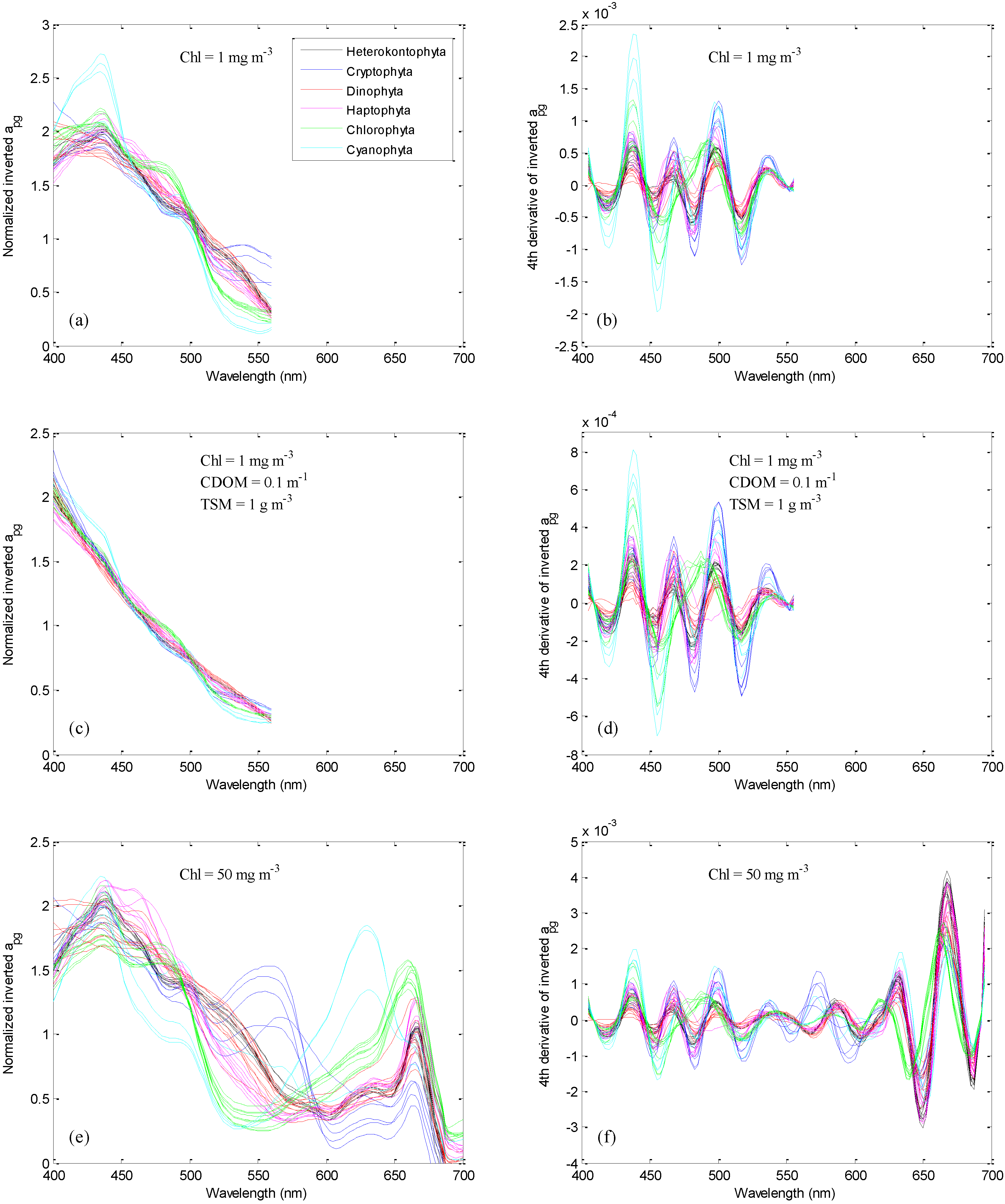
| apg_QAA(λ) (Chl = 1 mg∙m−3) | Mixed | 5/5 | 49/51 | 11/11 | ||
| apg_QAA(λ) (Chl = 1 mg∙m−3, CDOM = 0.1 m−1, TSM = 1 g∙m−3) | Mixed | 5/5 | 49/51 | 11/11 | ||
| apg_QAA(λ) (Chl = 50 mg∙m−3) | 29/30 | 18/21 | Undistinguishable | 5/5 | 51/51 | 11/11 |
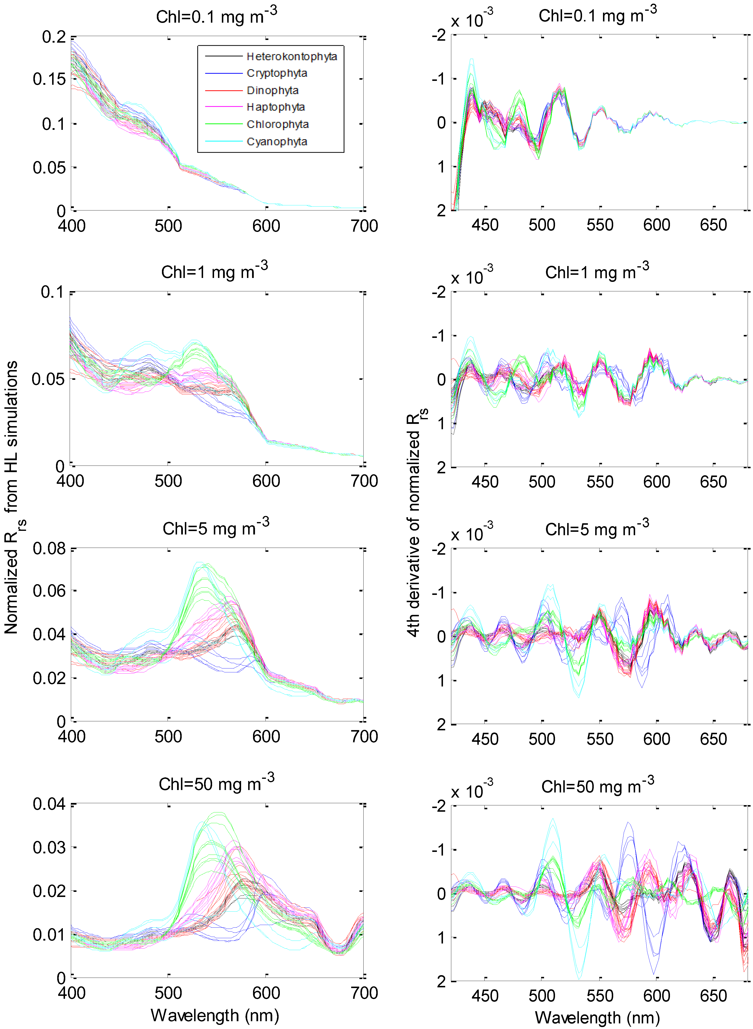
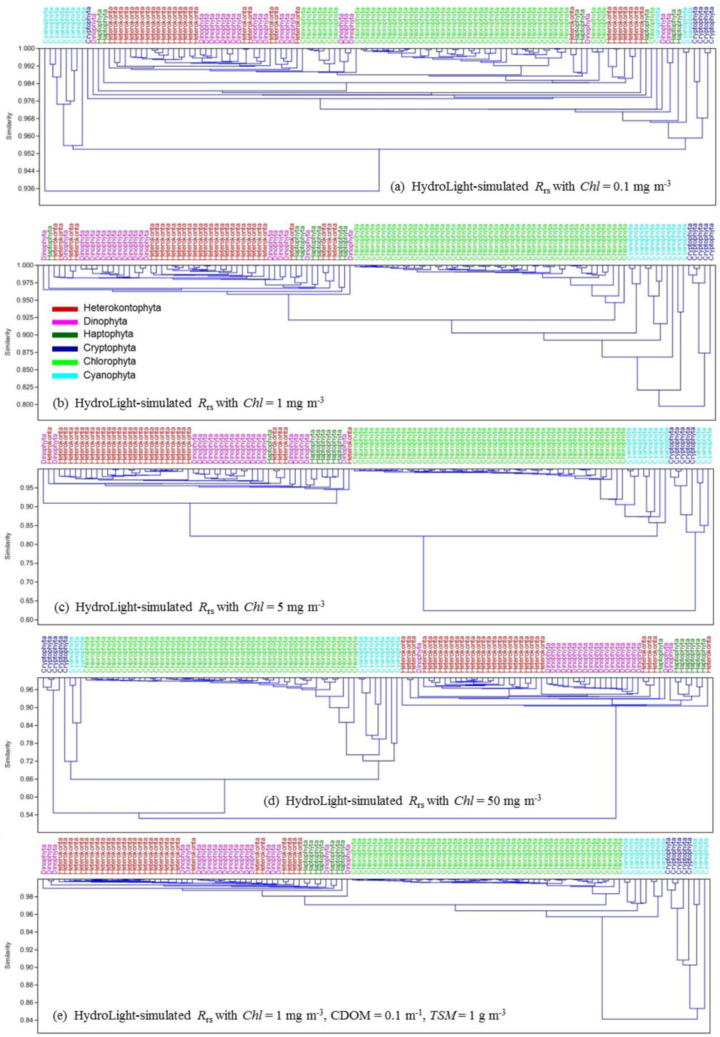
3.2. Derivative Analysis and Clustering on HydroLight-Simulated Rrs(λ)


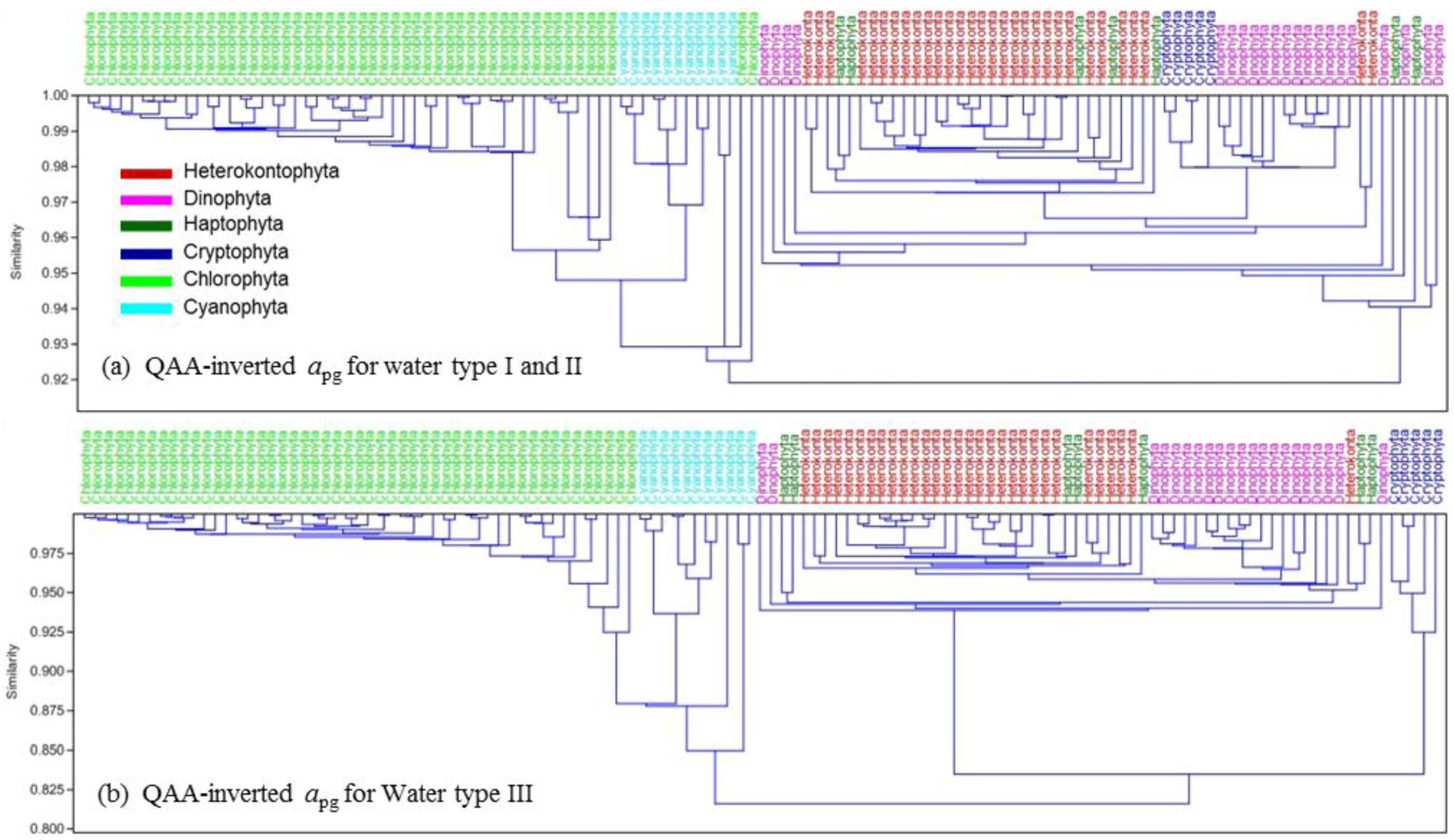
3.3. Phytoplankton Group Differentiation Using Absorption Inverted from Rrs(λ)

| Slope | R2 | RMSE (m−1) | N | |
|---|---|---|---|---|
| Water type I (Chl = 1 mg∙m−3) | 0.942 | 0.961 | 0.0086 | 500 |
| Water type II (Chl = 1 mg∙m−3, CDOM = 0.1 m−1, TSM = 1 g∙m−3) | 0.938 | 0.948 | 0.0245 | 500 |
| Water type III (Chl = 50 mg∙m−3, an extreme case) | 0.953 | 0.975 | 0.117 | 500 |

4. Discussion
4.1. HydroLight Simulations
4.2. Phytoplankton Groups Differentiation Using Absorption and Rrs(λ) Data—Performance Comparison
5. Conclusions and Outlook
Acknowledgments
Author Contributions
Conflicts of Interest
References
- Morel, A. Optical modelling of the upper ocean in relation to its biogenous matter content (case I waters). J. Geophys. Res. 1988, 93, 10749–10768. [Google Scholar] [CrossRef]
- O’Reilly, J.E.; Maritorena, S.; Mitchell, B.G.; Siegel, D.A.; Carder, K.L.; Garver, S.A.; Kahru, M.; McClain, C. Ocean color chlorophyll algorithms for SeaWiFS. J. Geophys. Res. 1998, 103, 24937–24953. [Google Scholar] [CrossRef]
- Maritorena, S.; Siegel, D.A.; Peterson, A. Optimization of a semi-analytical ocean color model for global scale applications. Appl. Opt. 2002, 41, 2705–2714. [Google Scholar] [CrossRef] [PubMed]
- Craig, S.E.; Lohrenz, S.E.; Lee, Z.; Mahoney, K.L.; Kirkpatrick, G.J.; Schofield, O.M.; Steward, R. Use of hyperspectral remote sensing reflectance for detection and assessment of the harmful alga, Karenia brevis. Appl. Opt. 2006, 45, 5414–5425. [Google Scholar] [CrossRef] [PubMed]
- Kutser, T.; Metsamaa, L.; Strömbeck, N.; Vahtmäe, E. Monitoring cyanobacterial blooms by satellite remote sensing. Estuar. Coast. Shelf Sci. 2006, 67, 303–312. [Google Scholar] [CrossRef]
- Astoreca, R.; Rousseau, V.; Ruddick, K.; Knechciak, C.; von Mol, B.; Parent, J.; Lancelot, C. Development and application of an algorithm for detecting Phaeocystis globosa blooms in the Case 2 Southern North Sea waters. J. Plankton Res. 2009, 31, 287–300. [Google Scholar] [CrossRef] [PubMed]
- Nair, A.; Sathyendranath, S.; Platt, T.; Morales, J.; Stuart, V.; Forget, M.-H.E.; Devred, E.; Bouman, H. Remote sensing of phytoplankton functional types. Remote Sens. Environ. 2008, 112, 3366–3375. [Google Scholar] [CrossRef]
- Bracher, A.; Hardman-Mountford, N. Overview on algorithms to derive phytoplankton community structure from satellite ocean colour. In Proceedings of the International Ocean Color Science (IOCS) Meeting, Darmstadt, Germany, 6–8 May 2013.
- Hirata, T.; Aiken, J.; Hardman-Mountford, N.; Smyth, T.J.; Barlow, R.G. An absorption model to determine phytoplankton size classes from satellite ocean color. Remote Sens. Environ. 2008, 112, 3153–3159. [Google Scholar] [CrossRef]
- Hirata, T.; Hardman-Mountford, N.J.; Brewin, R.J.W.; Aiken, J.; Barlow, R.; Suzuki, K.; Isada, T.; Howell, E.; Hashioka, T.; Aita-Noguchi, M.; et al. Synoptic relationships between surface Chlorophyll-a and diagnostic pigments specific to phytoplankton functional types. Biogeosciences 2011, 8, 311–327. [Google Scholar] [CrossRef]
- Brewin, R.J.W.; Sathyendranath, S.; Hirata, T.; Lavender, S.J.; Barciela, R.M.; Hardman-Mountford, N.J. A three-component model of phytoplankton size class for the Atlantic Ocean. Ecol. Modell. 2010, 221, 1472–1483. [Google Scholar] [CrossRef]
- Alvain, S.; Moulin, C.; Dandonneau, Y.; Breon, F.M. Remote sensing of phytoplankton groups in case 1 waters from global SeaWiFS imagery. Deep Sea Res. Part I 2005, 1, 1989–2004. [Google Scholar] [CrossRef] [Green Version]
- Alvain, S.; Moulin, C.; Dandonneau, Y. Seasonal distribution and succession of dominant phytoplankton groups in the global ocean: A satellite view. Glob. Biogeochem. Cycles 2008, 22. [Google Scholar] [CrossRef]
- Alvain, S.; Loisel, H.; Dessailly, D. Theoretical analysis of ocean color radiances anomalies and implications for phytoplankton groups detection in case 1 waters. Opt. Express 2012, 20, 1070–1083. [Google Scholar] [CrossRef] [PubMed]
- Ciotti, A.M.; Bricaud, A. Retrievals of a size parameter for phytoplankton and spectral light absorption by colored detrital matter from water-leaving radiances at SeaWiFS channels in a continental shelf region of Brazil. Limnol. Oceanog. Methods 2006, 4, 237–253. [Google Scholar] [CrossRef]
- Bricaud, A.; Ciotti, A.M.; Gentili, B. Spatial-temporal variations in phytoplankton size and colored detrital matter absorption at global and regional scales, as derived from twelve years of SeaWiFS data (1998–2009). Glob. Biogeochem. Cycles 2012, 26, GB1010. [Google Scholar] [CrossRef]
- Mouw, C.B.; Yoder, J.A. Optical determination of phytoplankton size composition from global SeaWiFS imagery. J. Geophys. Res. Ocean. 2010, 115, C12018. [Google Scholar] [CrossRef]
- Fujiwara, A.; Hirawake, T.; Suzuki, K.; Saitoh, S.I. Remote sensing of size structure of phytoplankton communities using optical properties of the Chukchi and Bering Sea shelf region. Biogeosciences 2011, 8, 3567–3580. [Google Scholar] [CrossRef]
- Organelli, E.; Bricaud, A.; Antoine, D.; Uitz, J. Multivariate approach for the retrieval of phytoplankton size structure from measured light absorption spectra in the Mediterranean Sea (BOUSSOLE site). Appl. Opt. 2013, 52, 2257–2273. [Google Scholar] [CrossRef] [PubMed]
- Bracher, A.; Vountas, M.; Dinter, T.; Burrows, J.P.; Röttgers, R.; Peeken, I. Quantitative observation of cyanobacteria and diatoms from space using PhytoDOAS on SCIAMACHY data. Biogeosciences 2009, 6, 751–764. [Google Scholar] [CrossRef]
- Sadeghi, A.; Dinter, T.; Vountas, M.; Taylor, B.B.; Altenburg-Soppa, M.; Peeken, I.; Bracher, A. Improvement to the PhytoDOAS method for identification of coccolithophores using hyper-spectral satellite data. Ocean Sci. 2012, 8, 1055–1070. [Google Scholar] [CrossRef] [Green Version]
- Kostadinov, T.S.; Siegel, D.A.; Maritorena, S. Retrieval of the particle size distribution from satellite ocean color observations. J. Geophys. Res. 2009, 114, C09015. [Google Scholar] [CrossRef]
- Lubac, B.; Loisel, H.; Guiselin, N.; Astoreca, R.; Artigas, L.F.; Meriaux, X. Hyperspectral and multispectral ocean color inversions to detect Phaeocystis globosa blooms in coastal waters. J. Geophys. Res. 2008, 113, C06026. [Google Scholar]
- Hunter, P.D.; Tyler, A.N.; Présing, M.; Kovács, A.W.; Preston, T. Spectral discrimination of phytoplankton colour groups: The effect of suspended particulate matter and sensor spectral resolution. Remote Sens. Environ. 2008, 112, 1527–1544. [Google Scholar] [CrossRef]
- Torrecilla, E.; Stramski, D.; Reynolds, R.A.; Millán-Núñez, E.; Piera, J. Cluster analysis of hyperspectral optical data for discriminating phytoplankton pigment assemblages in the open ocean. Remote Sens. Environ. 2011, 115, 2578–2593. [Google Scholar] [CrossRef] [Green Version]
- Taylor, B.B.; Torrecilla, E.; Bernhardt, A.; Taylor, M.H.; Peeken, I.; Röttgers, R.; Piera, J.; Bracher, A. Bio-optical provinces in the eastern Atlantic Ocean and their biogeographical relevance. Biogeosciences 2011, 8, 3609–3629. [Google Scholar] [CrossRef] [Green Version]
- Isada, T.; Hirawake, T.; Kobayashi, T.; Nosake, Y.; Natsuike, M.; Imai, I.; Suzuki, K.; Saitoh, S.-I. Hyperspectral optical discrimination of phytoplankton community structure in Funka Bay and its implications for ocean color remote sensing of diatoms. Remote Sens. Environ. 2015, 159, 134–151. [Google Scholar] [CrossRef]
- Guanter, L.; Kaufmann, H.; Segl, K.; Foerster, S.; Rogass, C.; Chabrillat, S.; Kuester, T.; Hollstein, A.; Rossner, G.; Chlebek, C.; et al. The EnMAP spaceborne imaging spectroscopy mission for Earth Observation. Remote Sens. 2015, 7, 8830–8857. [Google Scholar] [CrossRef]
- Hoepffner, N.; Sathyendranath, S. Effect of pigment composition on absorption properties of phytoplankton. Mar. Ecol. Prog. Ser. 1991, 73, 11–23. [Google Scholar] [CrossRef]
- Millie, D.F.; Schofield, O.M.; Kirpatrick, G.J.; Johnsen, G.; Tester, P.A.; Vinyard, B.T. Detection of harmful algal blooms using photopigments and absorption signatures: A case study of the Florida red tide dinoflagellate, Gymnodinium breve. Limnol. Oceanogr. 1997, 42, 1240–1251. [Google Scholar] [CrossRef]
- Millie, D.F.; Moline, M.A.; Schofield, O. Optical discrimination of a phytoplankton species in natural mixed populations. Limnol. Oceanogr. 2000, 45, 467–471. [Google Scholar] [CrossRef]
- Johnsen, G.; Samset, O.; Granskog, L.; Sakshaug, E. In vivo absorption characteristics in 10 classes of bloom-forming phytoplankton: Taxonomic characteristics and responses to photoadaptation by means of discriminant and HPLC analysis. Mar. Ecol. Prog. Ser. 1994, 105, 149–157. [Google Scholar] [CrossRef]
- Moberg, L.; Karlberg, B.; Sorensen, K.; Kallqvist, T. Assessment of phytoplankton class abundance using absorption spectra and chemometrics. Talanta 2002, 56, 153–160. [Google Scholar] [CrossRef]
- Hu, X.; Su, R.; Zou, W.; Ren, S.; Wang, H.; Chai, X.; Wang, Y. Research on the discrimination methods of algae based on the fluorescence excitation spectra. Acta Oceanol. Sin. 2010, 29, 116–128. [Google Scholar] [CrossRef]
- Smith, C.M.; Alberte, R.S. Characterization of in vivo absorption features of chorophyte, phaeophyte and rhodophyte algal species. Mar. Biol. 1994, 118, 511–521. [Google Scholar] [CrossRef]
- Roelke, D.L.; Kennedy, C.D.; Weidemann, A.D. Use of discriminant and fourth-derivative analysis with high-resolution absorption spectra for phytoplankton research: Limitations at varied signal-to-noise Ratio and spectral resolution. Gulf Mex. Sci. 1999, 2, 75–86. [Google Scholar]
- Millie, D.F.; Schofield, O.M.E.; Kirpatrick, G.J.; Johnsen, G.; Evens, T.J. Using absorbance and fluorescence spectra to discriminate microalgae. Eur. J. Phycol. 2002, 37, 313–322. [Google Scholar] [CrossRef]
- Beutler, M. Spectral Fluorescence of Chlorophyll and Phycobilins as an in-situ Tool of Phytoplankton Analysis–Models, Algorithms and Instruments. Ph.D. Thesis, Kiel University, Kiel, Germany, March 2013. [Google Scholar]
- Lee, Z.P.; Carder, K.L.; Arnone, R. Deriving inherent optical properties form water color: A multi-band quasianalytical algorithm for optically deep water. Appl. Opt. 2002, 41, 5755–5772. [Google Scholar] [CrossRef] [PubMed]
- Von Mol, B.; Ruddick, K.; Astoreca, R.; Park, Y.; Nechad, B. Optical detection of a Noctiluca scintillans bloom. EARSel eProc. 2007, 6, 130–137. [Google Scholar]
- Tao, B.; Pan, D.; Mao, Z.; Shen, Y.; Zhu, Q.; Chen, J. Optical detection of Prorocentrum donghaiense blooms based on multispectral reflectance. Acta Oceanol. Sin. 2013, 32, 48–56. [Google Scholar] [CrossRef]
- Shang, S.; Wu, J.; Huang, B.; Lin, G.; Lee, Z.; Liu, J.; Shang, S. A new approach to discriminate dinoflagellate from diatom blooms from space in the East China Sea. J. Geophys. Res. Ocean. 2014, 119, 4653–4668. [Google Scholar] [CrossRef]
- Werdell, P.J.; Roesler, C.S.; Goes, J.I. Discrimination of phytoplankton functional groups using an ocean reflectance inversion model. Appl. Opt. 2014, 53, 4833–4849. [Google Scholar] [CrossRef] [PubMed]
- Guillard, R.R.L. Culture of phytoplankton for feeding marine invertebrates. In Culture of Marine Invertebrate Animal; Smith, W.L., Chanley, M.H., Eds.; Plenum Press: New York, NY, USA, 1975; pp. 29–60. [Google Scholar]
- McFadden, G.I.; Melkonian, M. Use of Hepes buffer for microalgal culture media and fixation for electron microscopy. Phycologia 1986, 25, 551–557. [Google Scholar] [CrossRef]
- Röttgers, R.; Schönfeld, W.; Kipp, P.R.; Doerffer, R. Practical test of a point-source integrating cavity absorption meter: The performance of different collector assemblies. Appl. Opt. 2005, 44, 5549–5560. [Google Scholar] [CrossRef] [PubMed]
- Röttgers, R.; Häse, C.; Doerffer, R. Determination of the particulate absorption of microalgae using a point-source integrating-cavity absorption meter: Verification with a photometric technique, improvements for pigment bleaching and correction for chlorophyll fluorescence. Limnol. Oceanogr. Methods. 2007, 5, 1–12. [Google Scholar] [CrossRef]
- Roesler, C.S.; Perry, M.J.; Carder, K. Modeling in situ phytoplankton absorption from total absorption spectra in productive inland marine waters. Limnol. Oceangr. 1989, 34, 1510–1523. [Google Scholar] [CrossRef]
- Mobley, C.D. Light and Water: Radiative Transfer in Natural Waters; Academic Press: San Diego, CA, USA, 1994. [Google Scholar]
- Mobley, C.D.; Sundman, L.K. HydroLight 5.2—EcoLight 5.2 Users’ Guide; Sequoia Scientific, Inc: Bellevue, WA, USA, 2013. [Google Scholar]
- Bricaud, A.; Claustre, H.; Ras, J.; Oubelkheir, K. Natural variability of phytoplanktonic absorption in oceanic waters: Influence of the size structure of algal populations. J. Geophys. Res. 2004, 109, C11010. [Google Scholar] [CrossRef]
- Bricaud, A.; Morel, A.; Babin, M.; Allali, K.; Claustre, H. Variations of light absorption by suspended particles with chlorophyll-a concentration in oceanic (case 1) waters: Analysis and implications for bio-optical models. J. Geophys. Res. 1998, 103, 31033–31044. [Google Scholar] [CrossRef]
- Röttgers, R.; Doerffer, R.; Mckee, D.; Schönfeld, W. The Water Optical Properties Processor. Available online: http://calvalportal.ceos.org/data_access-tools (accessed on 18 February 2015).
- Petzold, T.J. Volume Scattering Functions for Selected Ocean Waters; SIO Ref. 72–78; Scripps Institution of Oceanography: La Jolla, CA, USA, 1972. [Google Scholar]
- Lee, Z.P.; Carder, K.L. Absorption spectrum of phytoplankton pigments derived from hyperspectral remote-sensing reflectance. Remote Sens. Environ. 2004, 89, 361–368. [Google Scholar] [CrossRef]
- Lee, Z.P.; Lubac, B.; Werdell, J.; Arnone, R. An Update of the Quasi-Analytical Algorithm (QAA_v5). Available online: http://www.ioccg.org/groups/software.html (accessed on 30 July 2014).
- Werdell, J.P.; Franz, B.A.; Bailey, S.W.; Feldman, G.C.; Boss, E.; Brando, V.E.; Dowell, M.; Hirata, T.; Lavender, S.J.; Lee, Z.P.; et al. A generalized ocean color inversion model for retrieving marine inherent optical properties. Appl. Opt. 2013, 52, 2019–2037. [Google Scholar] [CrossRef] [PubMed]
- Butler, W.L.; Hopkins, D.W. An analysis of fourth derivative spectra. Photochem. Photobiol. 1970, 12, 451–456. [Google Scholar] [CrossRef]
- Tsai, F.; Philpot, W.D. Derivative analysis of hyperspectral data. Remote Sens. Environ. 1998, 66, 41–51. [Google Scholar] [CrossRef]
- Torrecilla, E.; Piera, J.; Vilaseca, M. Derivative analysis of hyperspectral oceanographic data. In Advances in Geoscience and Remote Sensing; Jedlovec, G., Ed.; InTech: Rijeka, Croatia, 2009; pp. 597–618. [Google Scholar]
- Bidigare, R.R.; Morrow, J.H.; Kiefer, D.A. Derivative analysis of spectral absorption by photosynthetic pigments in the western Sargasso Sea. J. Mar. Res. 1989, 47, 323–341. [Google Scholar] [CrossRef]
- Savitzky, A.; Golay, M.J.E. Smoothing and differentiation of data by simplified least squares procedures. Anal. Chem. 1964, 36, 1627–1639. [Google Scholar] [CrossRef]
- Hammer, Ø.; Harper, D.A.T.; Ryan, P.D. PAST: Paleontological Statistics Software Package for Education and Data Analysis. Available online: http://palaeo-electronica.org/2001_1/past/issue1_01.htm (accessed on 10 February 2014).
- McKee, D.; Chami, M.; Brown, I.; Calzado, V.S.; Doxaran, D.; Cunningham, A. Role of measurement uncertainties in observed variability in the spectral backscattering ratio: A case study in mineral-rich coastal waters. Appl. Opt. 2009, 48, 4663–4675. [Google Scholar] [CrossRef] [PubMed]
- Tan, H.; Doerffer, R.; Oishi, T.; Tanaka, A. A new approach to measure the volume scattering function. Opt. Express 2013, 21, 18697–18711. [Google Scholar] [CrossRef] [PubMed]
- Mobley, C.D.; Sundman, L.K.; Boss, E. Phase function effects on oceanic light fields. Appl. Opt. 2002, 4, 1035–1050. [Google Scholar] [CrossRef]
- Dierssen, H.M.; Kudela, R.M.; Ryan, J.P.; Zimmerman, R.C. Red and black tides: Quantitative analysis of water—Leaving radiance and perceived color for phytoplankton, colored dissolved organic matter, and suspended sediments. Limnol. Oceanogr. 2006, 51, 2646–2659. [Google Scholar] [CrossRef]
- Twardowski, M.S.; Boss, E.; MacDonald, J.B.; Pegau, W.S.; Barnard, A.H.; Zaneveld, J.R.V. A model for estimating bulk refractive index from optical backscattering ratio and the implications for understanding particle composition in case I and case II waters. J. Geophys. Res. 2001, 106, 14129–14142. [Google Scholar] [CrossRef]
- Morel, A. Are the empirical relationships describing the bio-optical properties of case 1 waters consistent and internally compatible? J. Geophys. Res. Ocean. 2009, 114, C01016. [Google Scholar] [CrossRef]
- Tomlinson, M.C.; Stumpf, R.P.; Ransibrahmanakul, V.; Truby, E.W.; Kirkpatrick, G.J.; Pederson, B.A.; Vargo, G.A.; Heil, C.A. Evaluation of the use of SeaWiFS imagery for detecting Karenia brevis harmful algal blooms in the eastern Gulf of Mexico. Remote Sens. Environ. 2004, 91, 293–303. [Google Scholar] [CrossRef]
- Tomlinson, M.C.; Wynne, T.T.; Stumpf, R.P. An evolution of remote sensing techniques for enhanced detection of the toxic dinoflagellate, Karenia brevis. Remote Sens. Environ. 2009, 113, 598–609. [Google Scholar] [CrossRef]
- Cannizzaro, J.P.; Carder, K.L.; Chen, F.R.; Heil, C.A.; Vargo, G.A. A novel technique for detection of the toxic dinoflagellate, Karenia brevies, in the Gulf of Mexico from remotely sensed ocean color data. Cont. Shelf Res. 2008, 28, 137–158. [Google Scholar] [CrossRef]
© 2015 by the authors; licensee MDPI, Basel, Switzerland. This article is an open access article distributed under the terms and conditions of the Creative Commons Attribution license (http://creativecommons.org/licenses/by/4.0/).
Share and Cite
Xi, H.; Hieronymi, M.; Röttgers, R.; Krasemann, H.; Qiu, Z. Hyperspectral Differentiation of Phytoplankton Taxonomic Groups: A Comparison between Using Remote Sensing Reflectance and Absorption Spectra. Remote Sens. 2015, 7, 14781-14805. https://0-doi-org.brum.beds.ac.uk/10.3390/rs71114781
Xi H, Hieronymi M, Röttgers R, Krasemann H, Qiu Z. Hyperspectral Differentiation of Phytoplankton Taxonomic Groups: A Comparison between Using Remote Sensing Reflectance and Absorption Spectra. Remote Sensing. 2015; 7(11):14781-14805. https://0-doi-org.brum.beds.ac.uk/10.3390/rs71114781
Chicago/Turabian StyleXi, Hongyan, Martin Hieronymi, Rüdiger Röttgers, Hajo Krasemann, and Zhongfeng Qiu. 2015. "Hyperspectral Differentiation of Phytoplankton Taxonomic Groups: A Comparison between Using Remote Sensing Reflectance and Absorption Spectra" Remote Sensing 7, no. 11: 14781-14805. https://0-doi-org.brum.beds.ac.uk/10.3390/rs71114781