
Estimating Pasture Quality of Fresh Vegetation Based on Spectral Slope of Mixed Data of Dry and Fresh Vegetation—Method Development


Abstract
:
1. Introduction
2. Materials and Methods
2.1. Study Area
2.2. Data Collection and Spectral Measurements
2.3. Chemical Reference
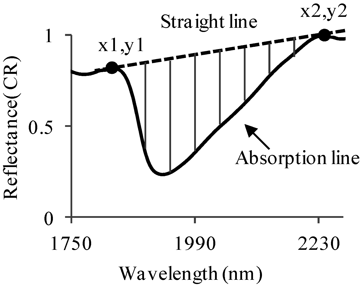
2.4. Slope Calculation and Data Analyses
2.5. Data Processing and Quantitative Analyses
2.6. PLS Data Analyses
2.7. Calculating the Water-Absorption Area

3. Results and Discussion
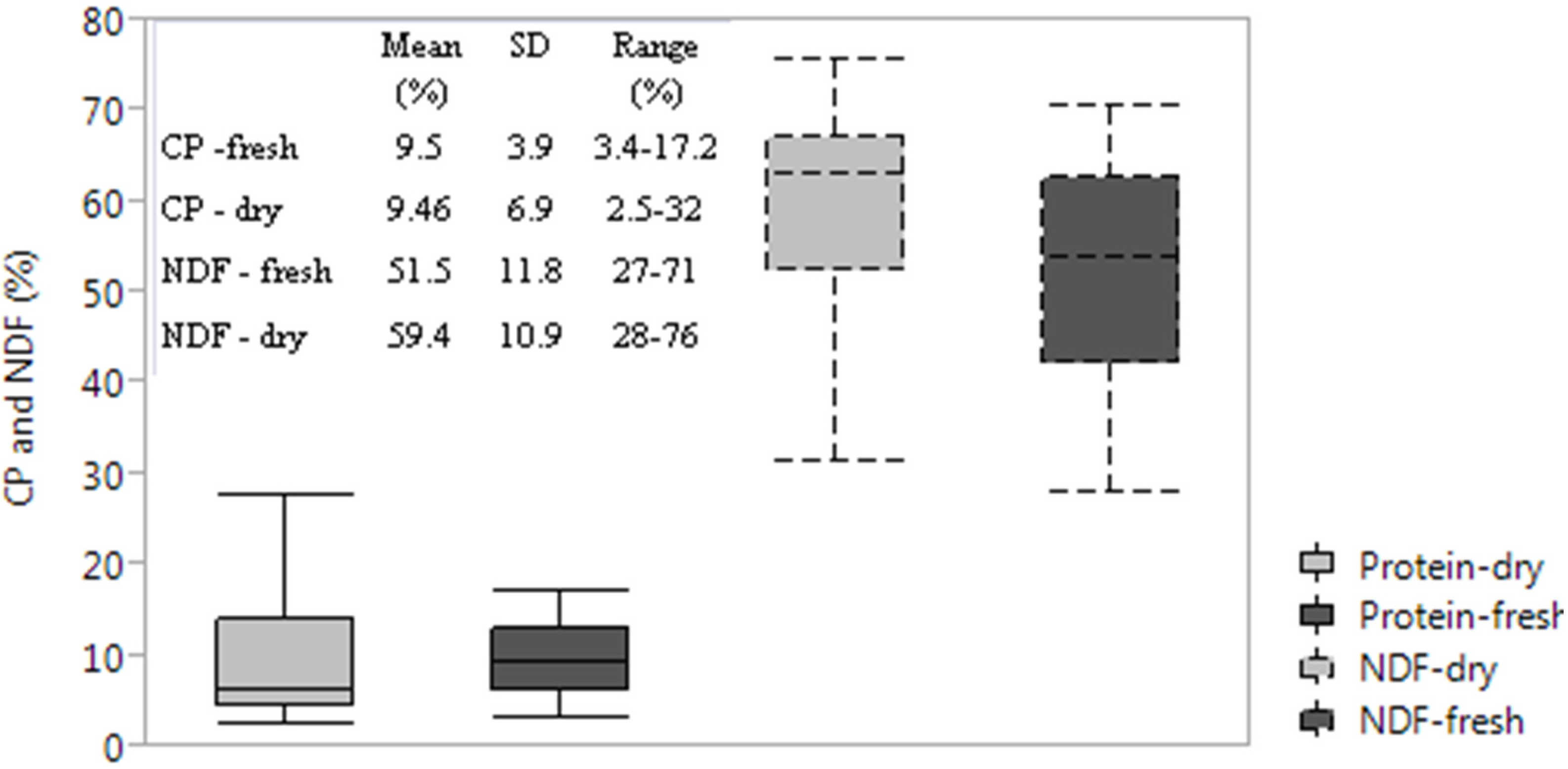
3.1. Chemical Reference: CP, NDF
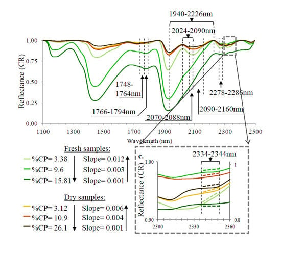
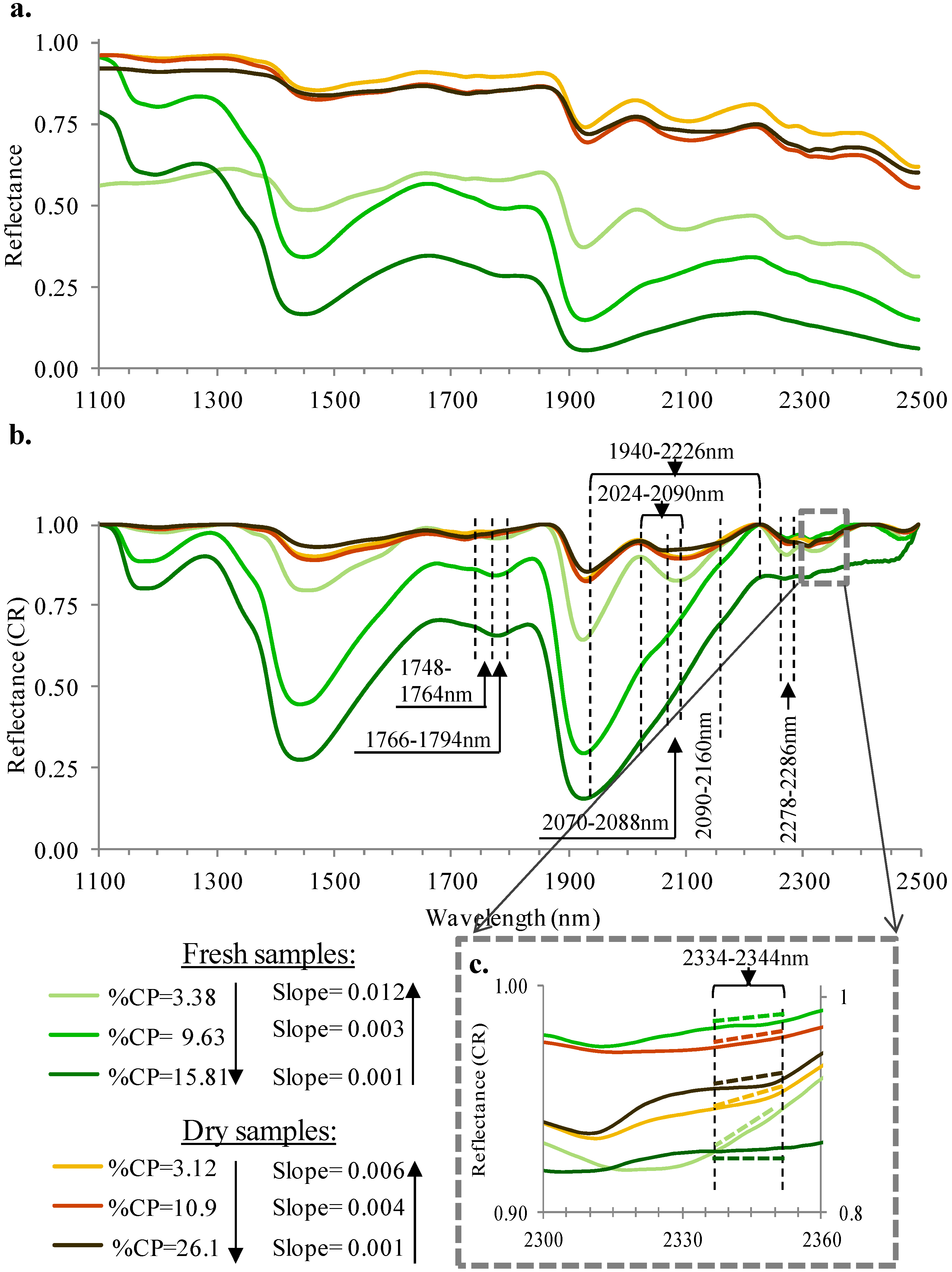
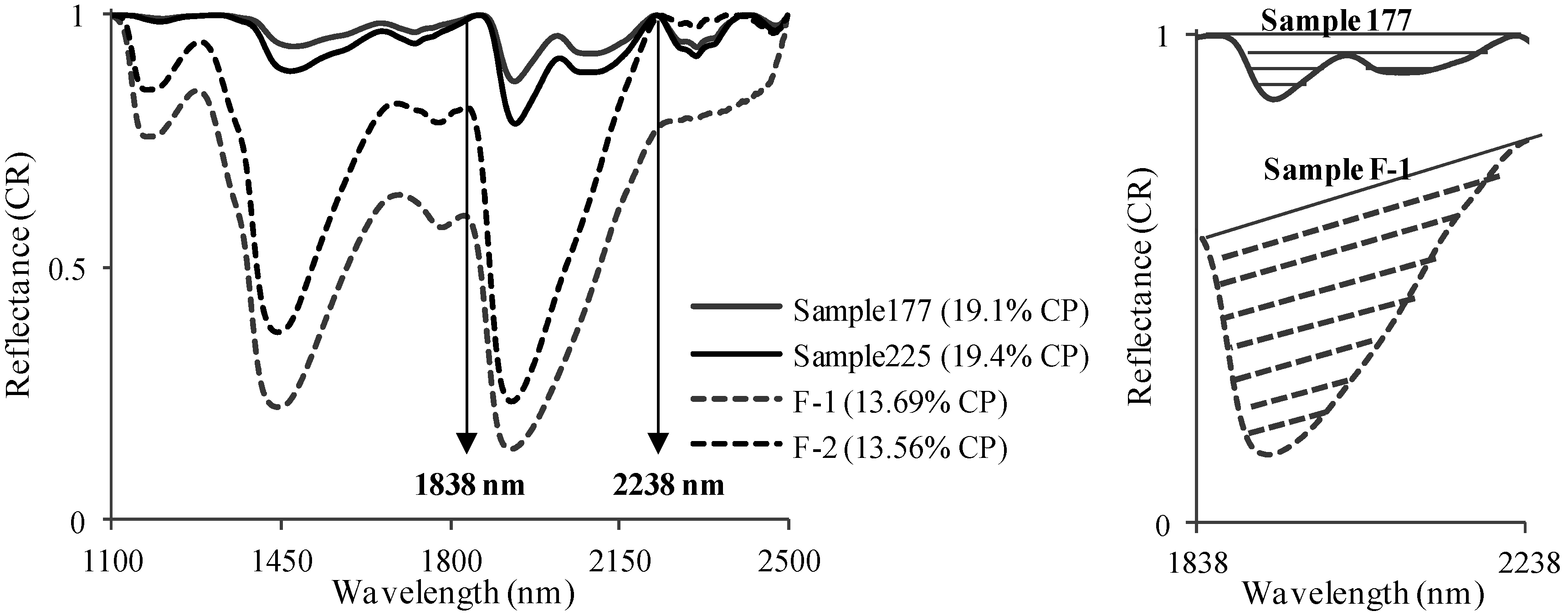
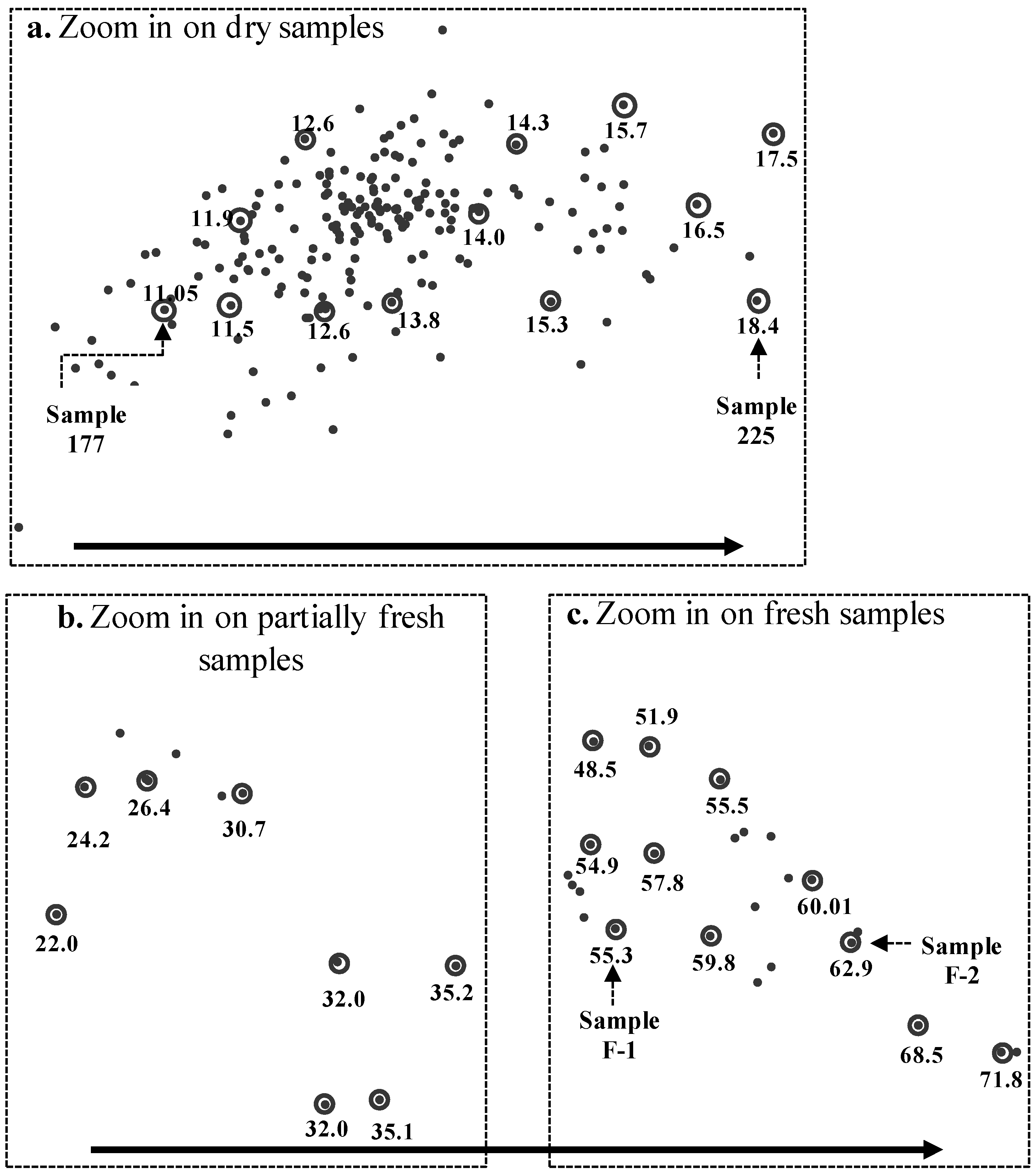
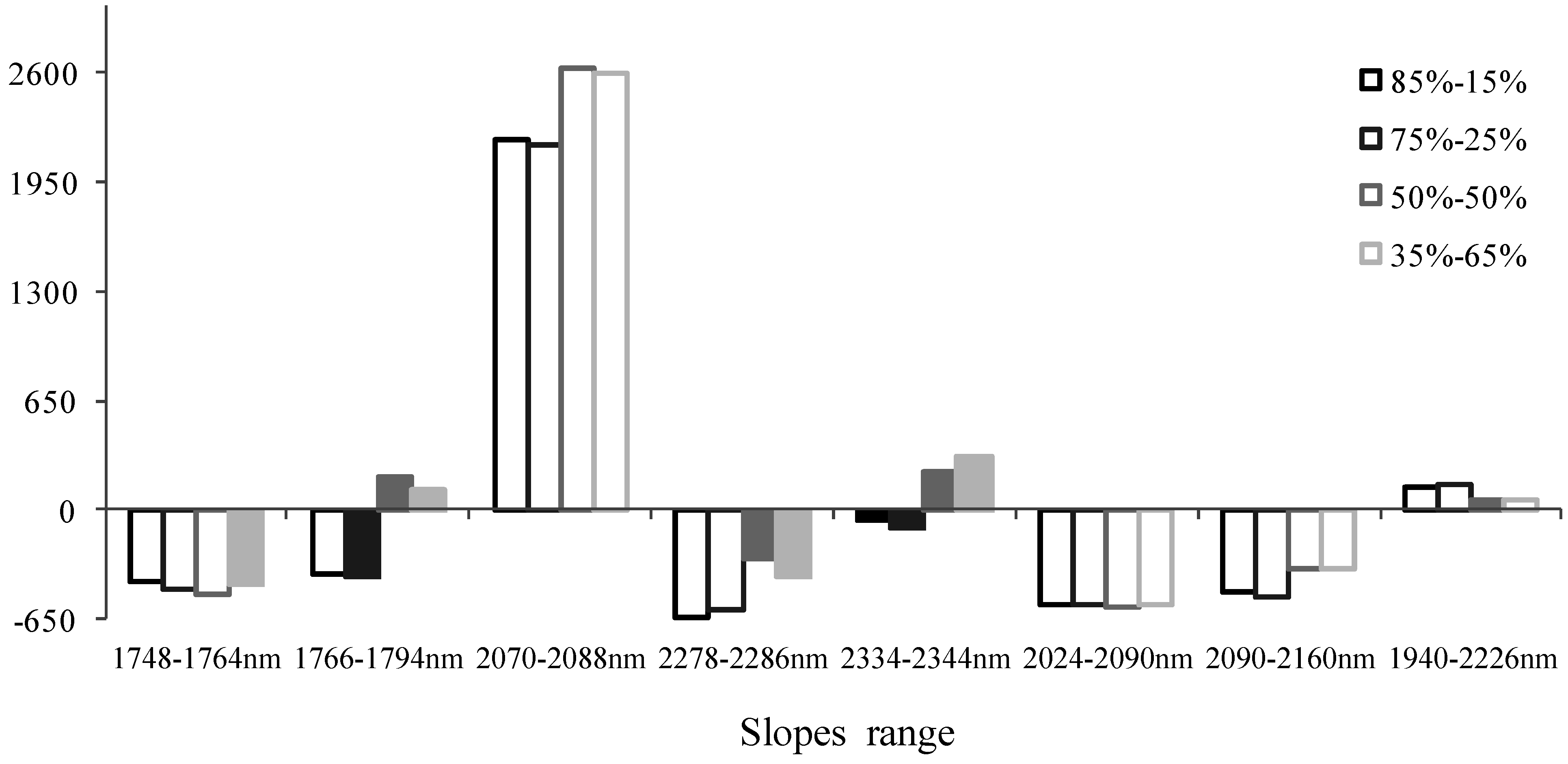
3.2. Spectral Slope Analysis


3.3. PLS Analysis

| CP | NDF | |
|---|---|---|
| Slope Spectral Range (nm) | R2 (n = 48) | R2 (n = 43) |
| 1748–1764 | 0.2804 | 0.1943 |
| 1766–1794 | 0.193 | 0.2258 |
| 2070–2088 | 0.4225 | 0.276 |
| 2278–2286 | 0.2415 | 0.3043 |
| 2334–2344 | 0.4149 | 0.4889 |
| 2090–2160 | 0.2387 | 0.15 |
| 2024–2090 | 0.3877 | 0.2422 |
| 1940–2226 | 0.1435 | 0.0884 |


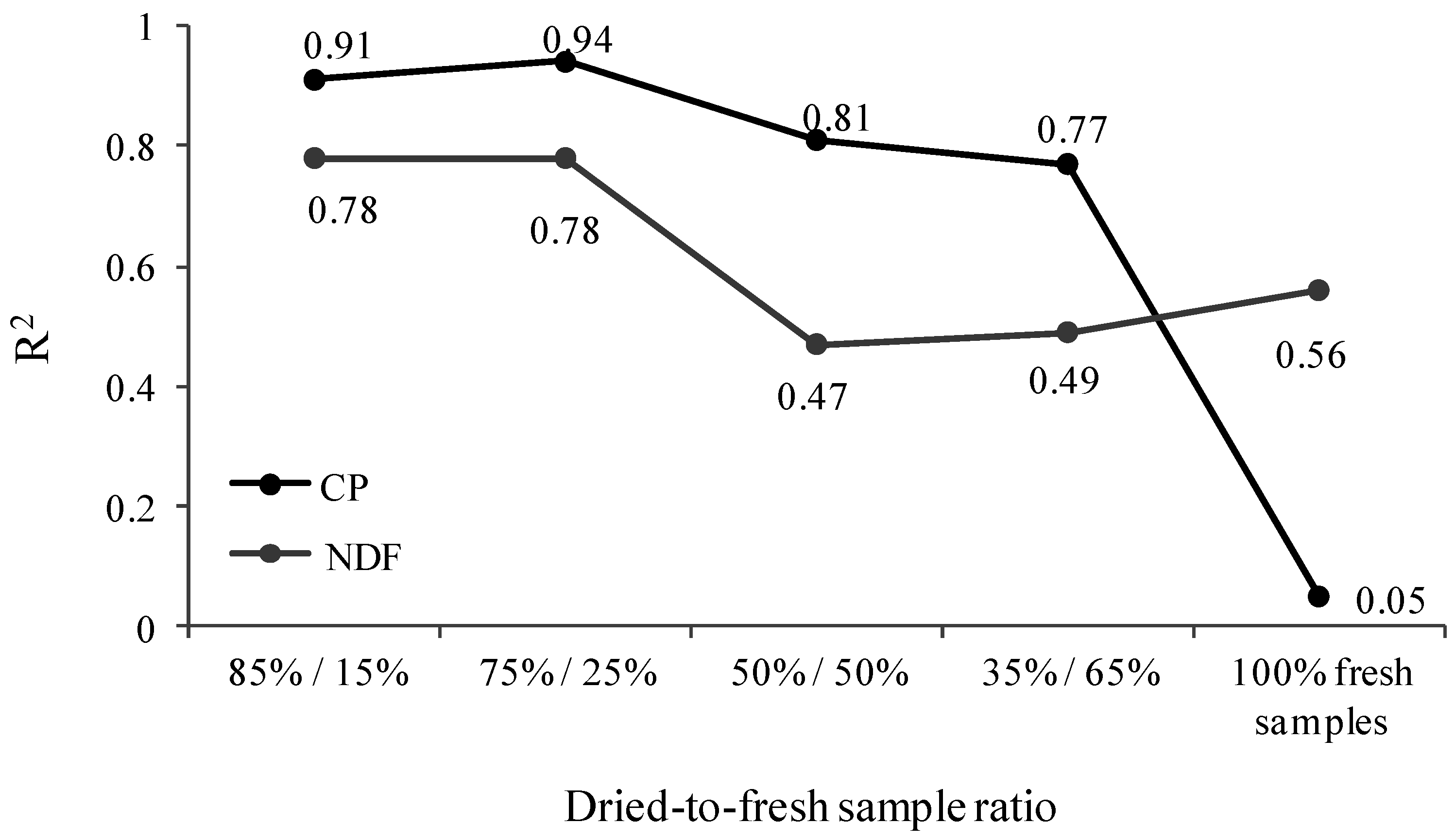
| CP Model Statistical Characteristics | NDF Model Statistical Characteristics | |||||||
|---|---|---|---|---|---|---|---|---|
| Calibration | Validation | Prediction | Calibration | Validation | Prediction | |||
| 100% Dry Samples | ||||||||
| Total dry samples | 198 | 198 | 26 | 197 | 197 | 35 | ||
| Slope | 0.95 | 0.94 | 0.99 | 0.96 | 0.96 | 0.98 | ||
| Offset | 0.34 | 0.36 | -0.15 | 1.56 | 1.60 | 0.32 | ||
| RMSE | 1.76 | 1.82 | 1.33 | 6.12 | 6.17 | 4.69 | ||
| RPD | 3.74 | 3.62 | 5.92 | 1.96 | 1.94 | 2.72 | ||
| R2 | 0.98 | 0.97 | 0.97 | 0.99 | 0.99 | 0.85 | ||
| 85%:15% (Dry/Fresh Samples) | ||||||||
| Total dry samples | 198 | 198 | 26 | 197 | 197 | 35 | ||
| Total fresh samples | 36 | 36 | 12 | 32 | 32 | 11 | ||
| Slope | 0.91 | 0.90 | 1.01 | 0.90 | 0.90 | 0.95 | ||
| Offset | 0.55 | 0.64 | -0.55 | 4.98 | 5.10 | 2.63 | ||
| RMSE | 2.34 | 2.52 | 1.45 | 7.49 | 7.57 | 4.75 | ||
| RPD | 2.50 | 2.70 | 4.80 | 1.68 | 1.67 | 2.59 | ||
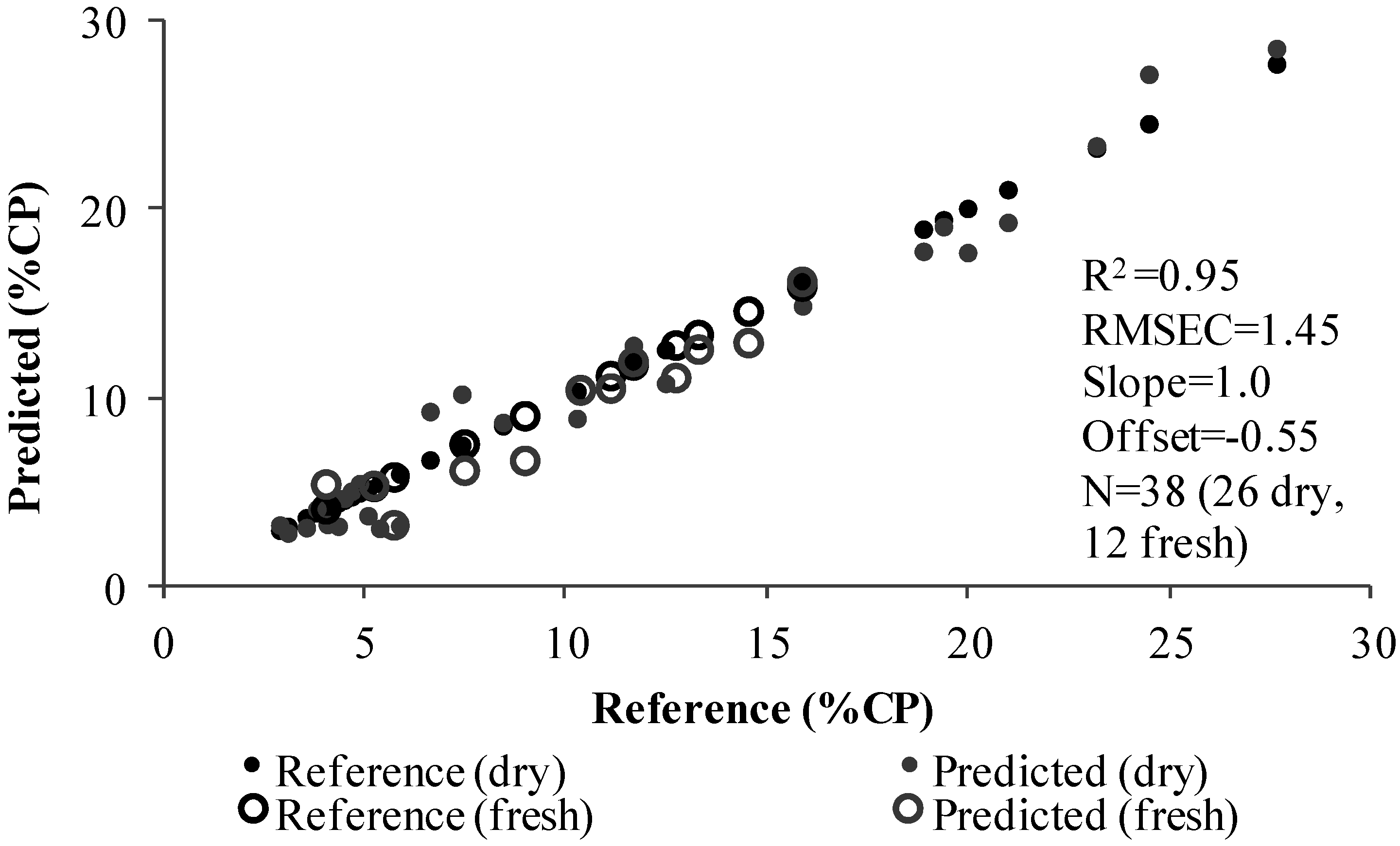
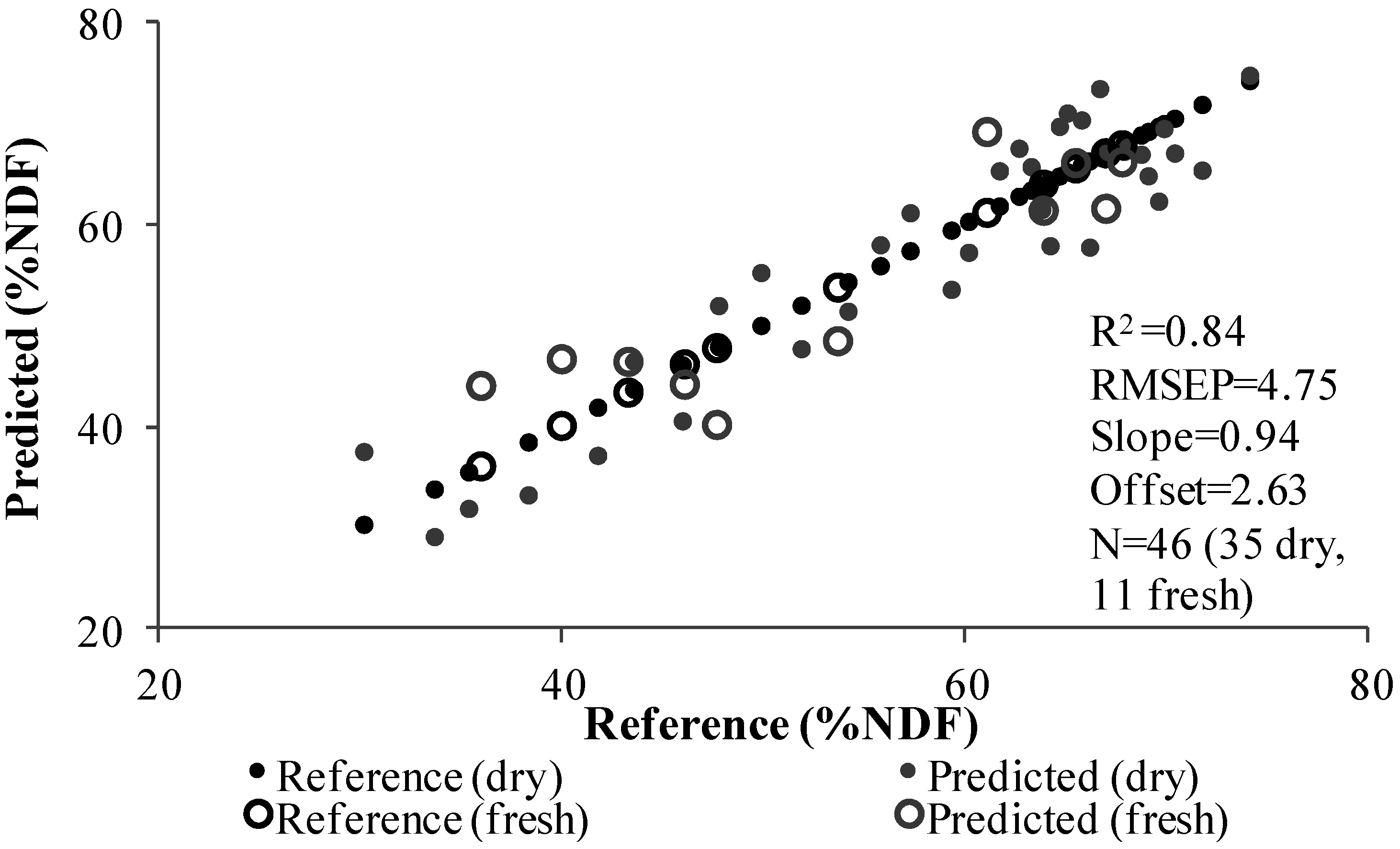
| R2 | 0.96 | 0.95 | 0.95 | 0.98 | 0.98 | 0.84 | ||
| 75%:25% (Dry/Fresh Samples) | ||||||||
| Total dry samples | 122 | 122 | 23 | 113 | 113 | 32 | ||
| Total fresh samples | 38 | 38 | 10 | 31 | 31 | 11 | ||
| Slope | 0.90 | 0.89 | 1.01 | 0.88 | 0.87 | 0.95 | ||
| Offset | 0.62 | 0.75 | -0.78 | 5.78 | 6.01 | 2.60 | ||
| RMSE | 2.63 | 2.82 | 1.26 | 8.18 | 8.32 | 4.63 | ||
| RPD | 2.43 | 2.27 | 5.15 | 1.59 | 1.57 | 2.49 | ||
| R2 | 0.95 | 0.94 | 0.95 | 0.98 | 0.97 | 0.82 | ||
| 50%:50% (Dry/Fresh Samples) | ||||||||
| Total dry samples | 42 | 42 | 10 | 43 | 43 | 10 | ||
| Total fresh samples | 38 | 38 | 10 | 32 | 32 | 10 | ||
| Slope | 0.89 | 0.86 | 0.92 | 0.78 | 0.77 | 0.97 | ||
| Offset | 0.64 | 0.99 | 0.43 | 11.2 | 11.7 | 3.01 | ||
| RMSE | 2.74 | 3.19 | 1.75 | 8.9 | 9.2 | 8.3 | ||
| RPD | 2.18 | 1.89 | 3.74 | 1.42 | 1.39 | 1.63 | ||
| R2 | 0.94 | 0.92 | 0.92 | 0.97 | 0.97 | 0.51 | ||
| 35%:65% (Dry/Fresh Samples) | ||||||||
| Total dry samples | 20 | 20 | 5 | 22 | 22 | 5 | ||
| Total fresh samples | 38 | 38 | 10 | 31 | 31 | 10 | ||
| Slope | 0.89 | 0.86 | 0.73 | 0.69 | 0.67 | 0.81 | ||
| Offset | 0.67 | 1.05 | 1.73 | 15.7 | 16.6 | 11.1 | ||
| RMSE | 2.88 | 3.36 | 2.14 | 9.69 | 9.99 | 8.43 | ||
| RPD | 2.15 | 1.87 | 1.97 | 1.27 | 1.23 | 1.55 | ||
| R2 | 0.94 | 0.91 | 0.72 | 0.96 | 0.96 | 0.50 | ||
| 100% Fresh Samples | ||||||||
| Total fresh samples | 38 | 38 | 10 | 33 | 33 | 10 | ||
| Slope | 0.4 | 0.38 | -0.08 | 0.47 | 0.48 | 0.58 | ||
| Offset | 5.32 | 5.54 | 11.7 | 25.47 | 25.6 | 23.9 | ||
| RMSE | 3.18 | 3.3 | 4.2 | 11.5 | 12.2 | 8.04 | ||
| RPD | 0.87 | 0.84 | 0.35 | 0.99 | 1.00 | 1.20 | ||
| R2 | 0.89 | 0.88 | NA | 0.95 | 0.94 | 0.56 | ||


4. Conclusion
Acknowledgments
Author Contributions
Conflicts of Interest
References
- Goering, H.K.; Van Soest, P.J. Forage fiber analysis (apparatus, reagents, procedures and some applications). In Agriculture Handbook No. 379; Agriculture Research Service, United States Department of Agriculture: Washington DC, USA, 1970; pp. 1–20. [Google Scholar]
- AOAC International. Official Methods of Analysis of AOAC International, 16th ed.; Association of Official Analytical Chemists: Arlington, VA, USA, 1995. [Google Scholar]
- Carey, W.P.; Wangen, E. Determining chemical characteristics of plutonium solutions using visible spectrometry and multivariate chemometric methods. Chemometrics Intelligent Lab. Syst. 1991, 10, 245–257. [Google Scholar] [CrossRef]
- Coscione, A.R.; Andrade, J.C.; van Raij, B.; Abreu, M.F. An improved analytical protocol for the routine spectrophotometric determination of exchangeable aluminum in soil extracts. Commun. Soil Sci. Plant Anal. 2000, 31, 2027–2037. [Google Scholar] [CrossRef]
- Evrendilek, F.I.C.; Kilic, S. Changes in soil organic carbon and other physical soil properties along adjacent Mediterranean forest, grassland, and cropland ecosystems. Turkey. J. Arid Environ. 2004, 59, 743–752. [Google Scholar] [CrossRef]
- Curran, P.J. Remote sensing of foliar chemistry. Remote Sens. Environ. 1989, 30, 271–278. [Google Scholar] [CrossRef]
- Murray, I.; Williams, P.C. Chemical principles of near infrared technology. In Near Infrared Technology in Agriculture and Food Industries; Wiliams, P.C., Noriss, K.H., Eds.; American Association of Cereal Chemistry Inc.: St. Paul, MN, USA, 1987; pp. 17–31. [Google Scholar]
- Workman, J., Jr.; Weyer, L. Practical Guide to Interpretive Near-Infrared Spectroscopy; CRC Press, Taylor & Francis Group: Boca Raton, FL, USA, 2008. [Google Scholar]
- Schwanninger, M.; Rodrigues, J.C.; Fackler, K. A review of band assignments in near infrared spectra of wood and wood components. J. Near Infrared Spectroscopy 2011, 19, 287–308. [Google Scholar] [CrossRef]
- Blanco, M.; Villarroya, I. NIR spectroscopy: a rapid-response analytical tool. Trends Anal. Chem. 2002, 21, 240–250. [Google Scholar] [CrossRef]
- Dematte, J.A.M.; Campos, R.C.; Alves, M.C.; Fiorio, P.R.; Nanni, M.R. Visible-NIR reflectance: a new approach on soil evaluation. Geoderma 2004, 12, 95–112. [Google Scholar] [CrossRef]
- Ben-Dor, E.; Banin, A. Near-infrared analysis as a method to simultaneously evaluate several soil properties. Soil Sci. Soc. Am. J. 1995, 59, 364–372. [Google Scholar] [CrossRef]
- Marten, G.C.; Brink, G.E.; Buxton, D.R.; Halgerson, J.L.; Hornstein, J.S. Near infrared reflectance spectroscopy analysis of forage quality in four legume species. Crop Sci. 1984, 24, 1179–1182. [Google Scholar] [CrossRef]
- Waters, C.J.; Givens, D.I. Nitrogen degradability of fresh herbage: effect of maturity and growth type, and prediction from chemical composition and by near infrared reflectance spectroscopy. Anim. Feed Sci. Technol. 1992, 38, 335–349. [Google Scholar] [CrossRef]
- Chudnovsky, A.; Ben-Dor, E.; Paz, E. Using NIRS for rapid assessment of sediment dust in the indoor environment. J. Near Infrared Spectroscopy 2007, 15, 59–70. [Google Scholar] [CrossRef]
- Chabrillat, S.; Ben-Dor, E.; Viscarra Rossel, R.A.; Demattê, J.A.M. Quantitative soil spectroscopy. Appl. Environ. Soil Sci. 2013. [Google Scholar] [CrossRef]
- Curran, P.J.; Kupiec, J.A.; Smith, G.M. Remote sensing the biochemical composition of a slash pine canopy. IEEE Trans. Geosci. Remote Sens. 1997, 35, 415–420. [Google Scholar] [CrossRef]
- Peterson, D.L.; Aber, J.D.; Matson, P.A.; Card, D.H.; Swanberg, N.; Wessman, C.; Spanner, M. Remote sensing of forest canopy and leaf biochemical contents. Remote Sens. Environ. 1988, 24, 85–108. [Google Scholar] [CrossRef]
- Wessman, C.A. Remote sensing and the estimation of ecosystem parameters and functions. In Imaging Spectrometry—A Tool for Environmental Observations; Hill, J., Megier, J., Eds.; Kluwer: Dordrecht, the Netherlands, 1994; pp. 39–56. [Google Scholar]
- Yoder, B.J.; Pettigrew-Crosby, R.E. Predicting nitrogen and chlorophyll content and concentrations from reflectance spectra (400–2500 nm) at leaf and canopy scales. Remote Sens. Environ. 1995, 53, 199–211. [Google Scholar] [CrossRef]
- Marten, G.C.; Shenk, J.S.; Barton, F.E., II. Near-Infrared Reflectance Spectroscopy (NIRS): Analysis of Forage Quality; United States Department of Agriculture Handbook 643; USDA: Washington, DC, USA, 1985; pp. 1–96.
- Norris, K.H.; Barners, R.F.; Moore, J.E.; Shenk, J.S. Predicting forage quality by infrared reflectance spectroscopy. J. Anim. Sci. 1976, 43, 889–897. [Google Scholar]
- Garcia, J.; Cozzolino, D. Use of near infrared reflectance (NIR) spectroscopy to predict chemical composition of forages in broad-based calibration models. Agricultura Técnica 2006, 66, 41–47. [Google Scholar] [CrossRef]
- Landau, S.; Friedman, S.; Brenner, S.; Bruckental, I.; Weinberg, Z.G.; Ashbell, G.; Hen, Y.; Dvash, L.; Leshem, Y. The value of safflower (Carthamus tinctorius) hay and silage grown under Mediterranean conditions as forage for dairy cattle. Livestock Prod. Sci. 2004, 88, 263–271. [Google Scholar] [CrossRef]
- Landau, S.; Glasser, T.; Dvash, L. Monitoring nutrition in small ruminants by aids of near infrared spectroscopy (NIRS) technology: A review. Small Ruminant Res. 2006, 61, 1–11. [Google Scholar] [CrossRef]
- Landau, S.; Nitzan, R.; Barkai, D.; Dvash, L. Excretal near infrared reflectance spectrometry to monitor the nutrient content of diets of grazing young ostriches (Struthio camelus). South African J. Anim. Sci. 2006, 36, 248–256. [Google Scholar]
- Landau, S.; Giger-Reverdin, S.; Rapetti, L.; Dvash, L.; Dorleans, M.; Ungar, E.D. Data mining old digestibility trials for nutritional monitoring in confined goats with aids of fecal near infra-red spectrometry. Small Ruminant Res. 2008, 77, 146–158. [Google Scholar] [CrossRef]
- Lugassi, R.; Chudnovsky, A.; Zaady, E.; Dvash, L.; Goldshleger, N. Spectral slope as an indicator of pasture quality. Remote Sens. 2015, 7, 256–274. [Google Scholar] [CrossRef]
- Decruyenaere, V.; Lecomte, P.; Demarquilly, C.; Aufrere, J.; Dardenne, P.; Stilmant, D.; Buldgen, A. Evaluation of green forage intake and digestibility in ruminants using near infrared reflectance spectroscopy (NIRS): Developing a global calibration. Anim. Feed Sci. Technol. 2009, 148, 138–156. [Google Scholar] [CrossRef]
- Cozzolino, D. Use of infrared spectroscopy for in-field measurement and phenotyping of plant properties: instrumentation, data analysis, and examples. Appl. Spectroscopy Rev. 2014, 49, 564–584. [Google Scholar] [CrossRef]
- Petisco, C.; García-Criado, B.; García-Criado, L.; Vázquez-de-Aldana, B.R.; García-Ciudad, A. Quantitative analysis of chlorophyll and protein in alfalfa leaves using fiber-optic near-infrared spectroscopy. Comm. Soil Sci. Plant Anal. 2009, 40, 2474–2484. [Google Scholar] [CrossRef]
- Cozzolino, D.; Labandera, M. Determination of dry matter and crude protein contents of undried forages by near-infrared reflectance spectroscopy. J. Sci. Food Agric. 2002, 82, 380–384. [Google Scholar] [CrossRef]
- Dardenne, P.; Agneessens, R.; Sinnaeve, G. Fresh forage analysis by near infrared spectroscopy. In Near Infrared Spectroscopy: The Future Waves; Davies, A.M.C., Williams, P., Eds.; NIR Publications: Chichester, UK, 1996; pp. 531–536. [Google Scholar]
- De la Roza, B.; Martínez, A.; Modroño, S.; Santos, B. Determination of the quality of fresh silages by near infrared reflectance spectroscopy. In Near Infrared Spectroscopy: The Future Waves; Davies, A.M.C., Williams, P., Eds.; NIR Publications: Chichester, UK, 1996; pp. 537–541. [Google Scholar]
- Pullanagari, R. Proximal Sensing Techniques to Monitor Pasture Quality and Quantity on Dairy Farms. Ph.D. Thesis, Massey University, Manawatu, New Zealand, 2011. [Google Scholar]
- Pullanagari, R.; Yule, I.; Tuohy, M.; Hedley, M.; Dynes, R.; King, W. In-field hyperspectral proximal sensing for estimating quality parameters of mixed pasture. Precision Agric. 2012, 13, 351–369. [Google Scholar] [CrossRef]
- Pullanagari, R.; Yule, I.; Tuohy, M.; Hedley, M.; Dynes, R.; King, W. Multi-spectral radiometry to estimate pasture quality components. Precision Agric. 2012, 13, 442–456. [Google Scholar] [CrossRef]
- Israel Forecast. Available online: http://www.ims.gov.il/IMSEng/ (accessed on 14 June 2015).
- Stern, A.; Gradus, Y.; Meir, A.; Krakover, S.; Tsoar, H. Atlas of the Negev; Ben Gurion University of the Negev: Beer-Sheva, Israel, 1986. [Google Scholar]
- Dan, J.; Yaalon, D.; Kundzimzinsky, H.; Raz, Z. The Soil of Israel; ARO Publication Bulletin No. 168 (in Hebrew). Agricultural Research Organization: Bet Dagan, Israel, 1977. [Google Scholar]
- Zaady, E.; Levacov, R.; Shachak, M. Application of the herbicide, Simazine, and its effect on soil surface parameters and vegetation in a patchy desert landscape. Arid Land Res. Manage. 2004, 18, 397–410. [Google Scholar] [CrossRef]
- Feinbrun-Dothan, N.; Danin, A. Analytical Flora of Eretz-Israel; Cana Publishers: Jerusalem, Israel, 1991. [Google Scholar]
- Zaady, E.; Yonatan, R.; Shachak, M.; Perevolotsky, A. The effects of grazing on abiotic and biotic parameters in a semiarid ecosystem: a case study from the northern Negev desert, Israel. Arid Land Res. Manage. 2001, 15, 245–261. [Google Scholar] [CrossRef]
- Henkin, Z.; Landau, S.; Ungar, E.D.; Perevolotsky, A.; Yehuda, Y.; Sternberg, M. Effect of timing and intensity of grazing on the herbage quality of a Mediterranean rangeland. J. Anim. Feed Sci. 2007, 16, 318–322. [Google Scholar]
- Henkin, Z.; Ungar, E.D.; Dvash, L.; Perevolotsky, A.; Yehuda, Y.; Sternberg, M.; Voet, H.; Landau, S.Y. Effects of cattle grazing on herbage quality in a herbaceous Mediterranean rangeland. Grass Forage Sci. 2011, 66, 516–525. [Google Scholar] [CrossRef]
- Tilley, J.M.A.; Terry, R.A. A two-stage technique for the in vitro digestion of forage crops. J. Br. Grassl. Soc. 1963, 18, 104–111. [Google Scholar] [CrossRef]
- Van Soest, P.J.; Robertson, J.B.; Lewis, B.A. Methods for dietary fiber, neutral detergent fiber and non-starch polysaccharides in relation to animal nutrition. J. Dairy Sci. 1991, 74, 3583–3597. [Google Scholar] [CrossRef]
- Kokaly, R.F.; Clark, R.N. Spectroscopic determination of leaf biochemistry using band-depth analysis of absorption features and stepwise multiple linear regression. Remote Sens. Environ. 1999, 67, 267–287. [Google Scholar] [CrossRef]
- Kokaly, R.F. Investigating a physical basis for spectroscopic estimates of leaf nitrogen concentration. Remote Sens. Environ. 2001, 75, 153–161. [Google Scholar] [CrossRef]
- Mutanga, O.; Skidmore, A.K. Narrow band vegetation indices overcome the saturation problem in biomass estimation. Int. J. Remote Sens. 2004, 25, 3999–4014. [Google Scholar] [CrossRef]
- Noomen, M.F.; Skidmore, A.K.; van der Meer, F.D.; Prins, H.H.T. Continuum removed band depth analysis for detecting the effects of natural gas, methane and ethane on maize reflectance. Remote Sens. Environ. 2006, 105, 262–270. [Google Scholar] [CrossRef]
- Esbensen, K. Multivariate Data Analyses in Practice—An Introduction to Multivariate Data Analyses and Experimental Design; Aalborg University, CAMO: Esbjerg, Denmark, 2002. [Google Scholar]
- Wold, S.; Sjostrom, M.; Eriksson, L. PLS-regression: A basic tool of chemometrics. Chemometrics Intelligent Lab. Syst. 2001, 58, 109–130. [Google Scholar] [CrossRef]
- Goldshleger, N.; Chudnovsky, A.; Ben-Binyam, R. Predicting salinity in tomato using soil reflectance spectra. Int. J. Remote Sens. 2013, 34, 6079–6093. [Google Scholar] [CrossRef]
- Jensen, J.R. Remote sensing of vegetation. In Remote Sensing of the Environment: An Earth Resource Perspective; Prentice Hall: Upper Saddle River, NJ, USA, 2007; pp. 355–408. [Google Scholar]
- Clark, R.N.; Roush, T.L. Reflectance spectroscopy: quantitative analysis techniques for remote sensing applications. J. Geophys. Res. 1984, 89, 6329–6340. [Google Scholar] [CrossRef]
- Duckworth, J. Mathematical data processing. In Near-Infrared Spectroscopy in Agriculture; Roberts, C.A., Workman, J., Jr., Reeves, J.B., Eds.; American Society of Agronomy, Crop Science Society of America, Soil Science Society of America: Madison, WI, USA, 2004; pp. 115–132. [Google Scholar]
- Mark, H. Quantitative spectroscopic calibration. In Encyclopedia of Analytical Chemistry: Applications, Theory, and Instrumentation; Meyers, R.A., Ed.; John Wiley & Sons Ltd.: Chichester, UK, 2000; pp. 13587–13605. [Google Scholar]
- Guo, X.; Wilmshurst, J.F.; Li, Z. Comparison of laboratory and field remote sensing methods to measure forage quality. Int. J. Environ. Res. Public Health 2010, 7, 3513–3530. [Google Scholar] [CrossRef] [PubMed]
- Starks, P.J.; Coleman, S.W.; Phillips, W.A. Determination of forage chemical composition using remote sensing. J. Range Manage. 2004, 57, 635–640. [Google Scholar] [CrossRef]
- Zhao, D.; Starks, P.J.; Brown, M.A.; Phillips, W.A.; Coleman, S.W. Assessment of forage biomass and quality parameter of bermudagrass using proximal sensing of pasture canopy reflectance. Grassland Sci. 2007, 53, 39–49. [Google Scholar] [CrossRef]
- Adjorlolo, C.; Mutanga, O.; Cho, M.O. Predicting C3 and C4 grass nutrient variability using in situ canopy reflectance and partial least squares regression. Int. J. Remote Sens. 2015, 36, 1743–1761. [Google Scholar] [CrossRef]
© 2015 by the authors; licensee MDPI, Basel, Switzerland. This article is an open access article distributed under the terms and conditions of the Creative Commons Attribution license (http://creativecommons.org/licenses/by/4.0/).
Share and Cite
Lugassi, R.; Chudnovsky, A.; Zaady, E.; Dvash, L.; Goldshleger, N. Estimating Pasture Quality of Fresh Vegetation Based on Spectral Slope of Mixed Data of Dry and Fresh Vegetation—Method Development. Remote Sens. 2015, 7, 8045-8066. https://0-doi-org.brum.beds.ac.uk/10.3390/rs70608045
Lugassi R, Chudnovsky A, Zaady E, Dvash L, Goldshleger N. Estimating Pasture Quality of Fresh Vegetation Based on Spectral Slope of Mixed Data of Dry and Fresh Vegetation—Method Development. Remote Sensing. 2015; 7(6):8045-8066. https://0-doi-org.brum.beds.ac.uk/10.3390/rs70608045
Chicago/Turabian StyleLugassi, Rachel, Alexandra Chudnovsky, Eli Zaady, Levana Dvash, and Naftaly Goldshleger. 2015. "Estimating Pasture Quality of Fresh Vegetation Based on Spectral Slope of Mixed Data of Dry and Fresh Vegetation—Method Development" Remote Sensing 7, no. 6: 8045-8066. https://0-doi-org.brum.beds.ac.uk/10.3390/rs70608045