
Semi-Global Filtering of Airborne LiDAR Data for Fast Extraction of Digital Terrain Models


Abstract
:
1. Introduction
2. Semi-Global Filtering
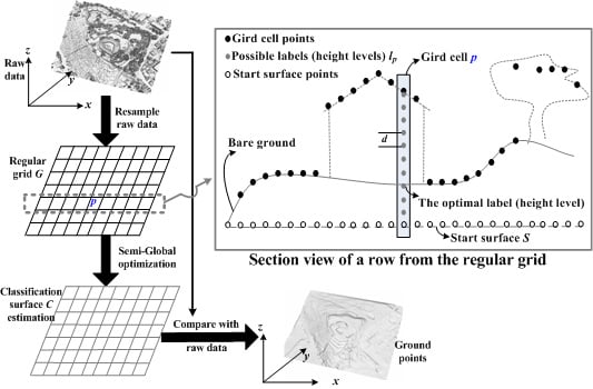
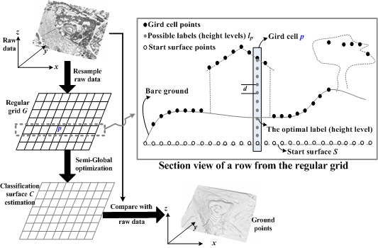
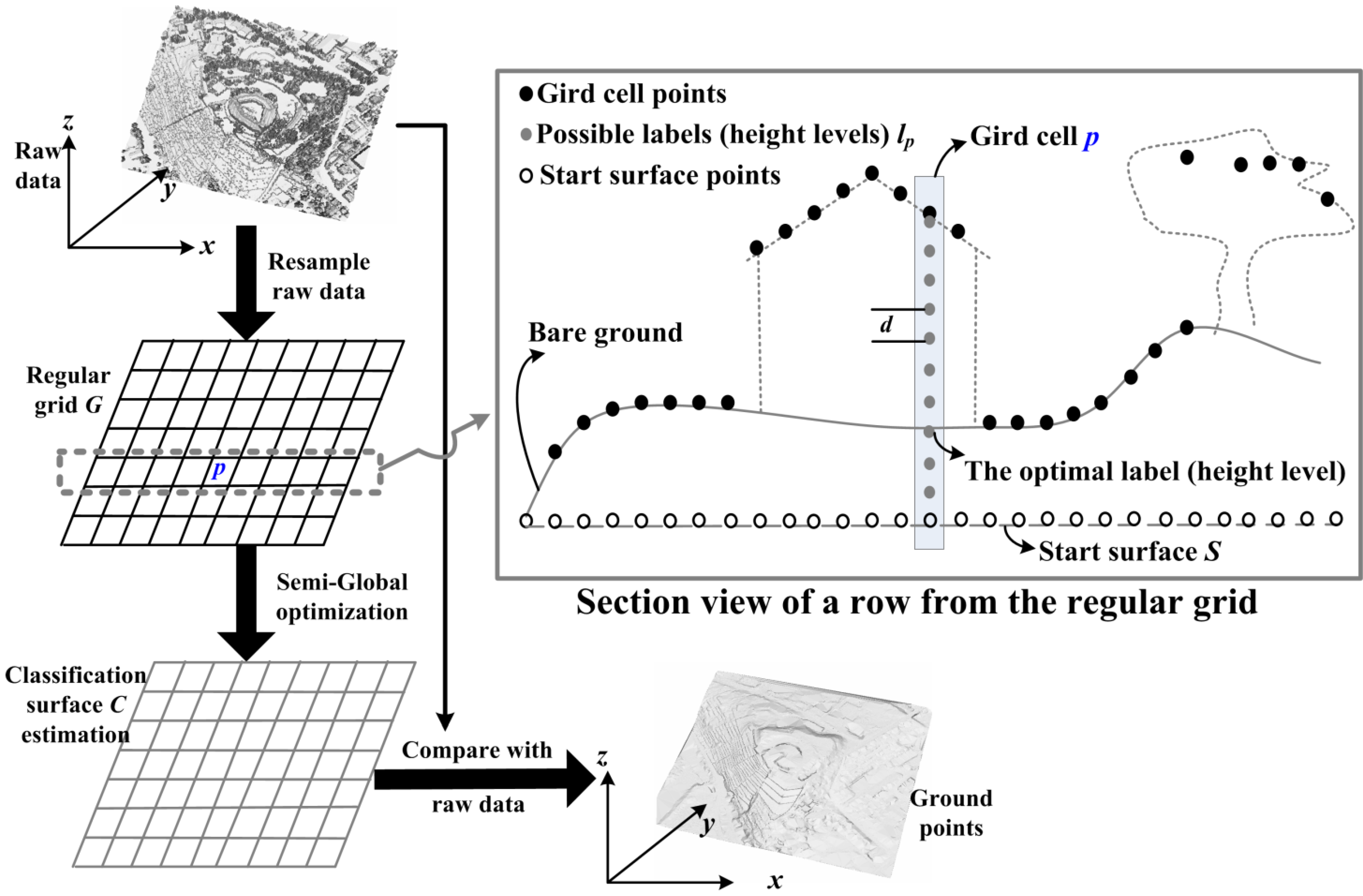
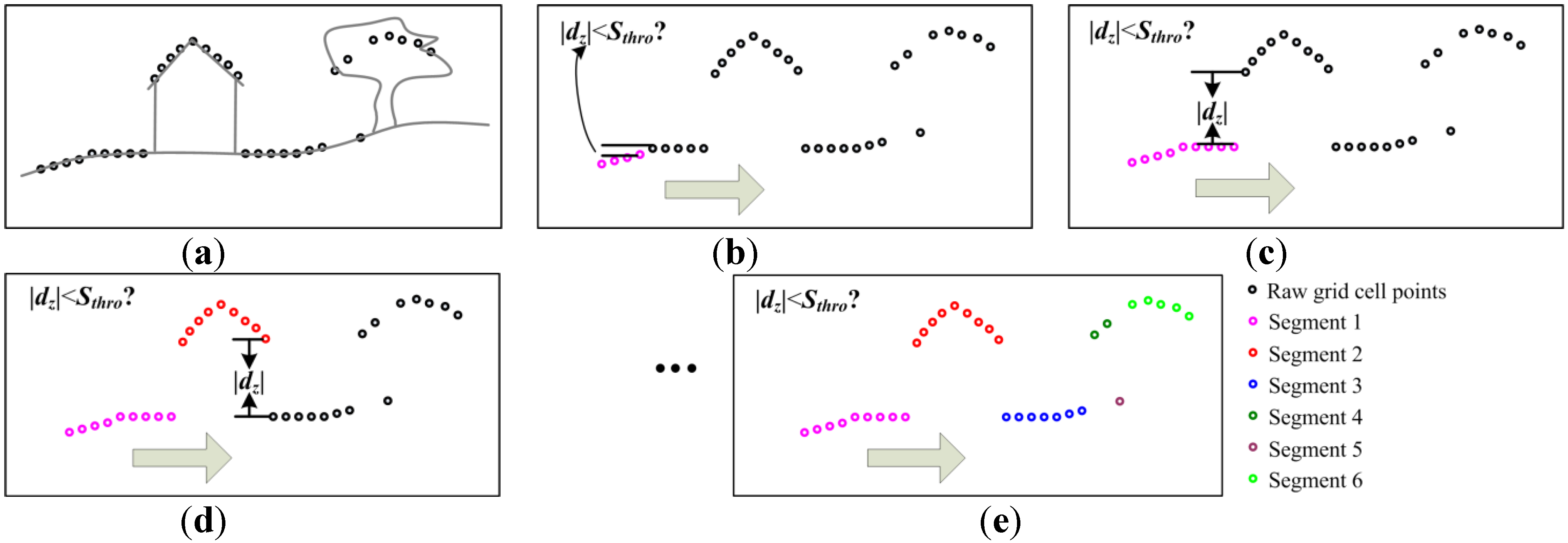
2.1. Algorithm Overview


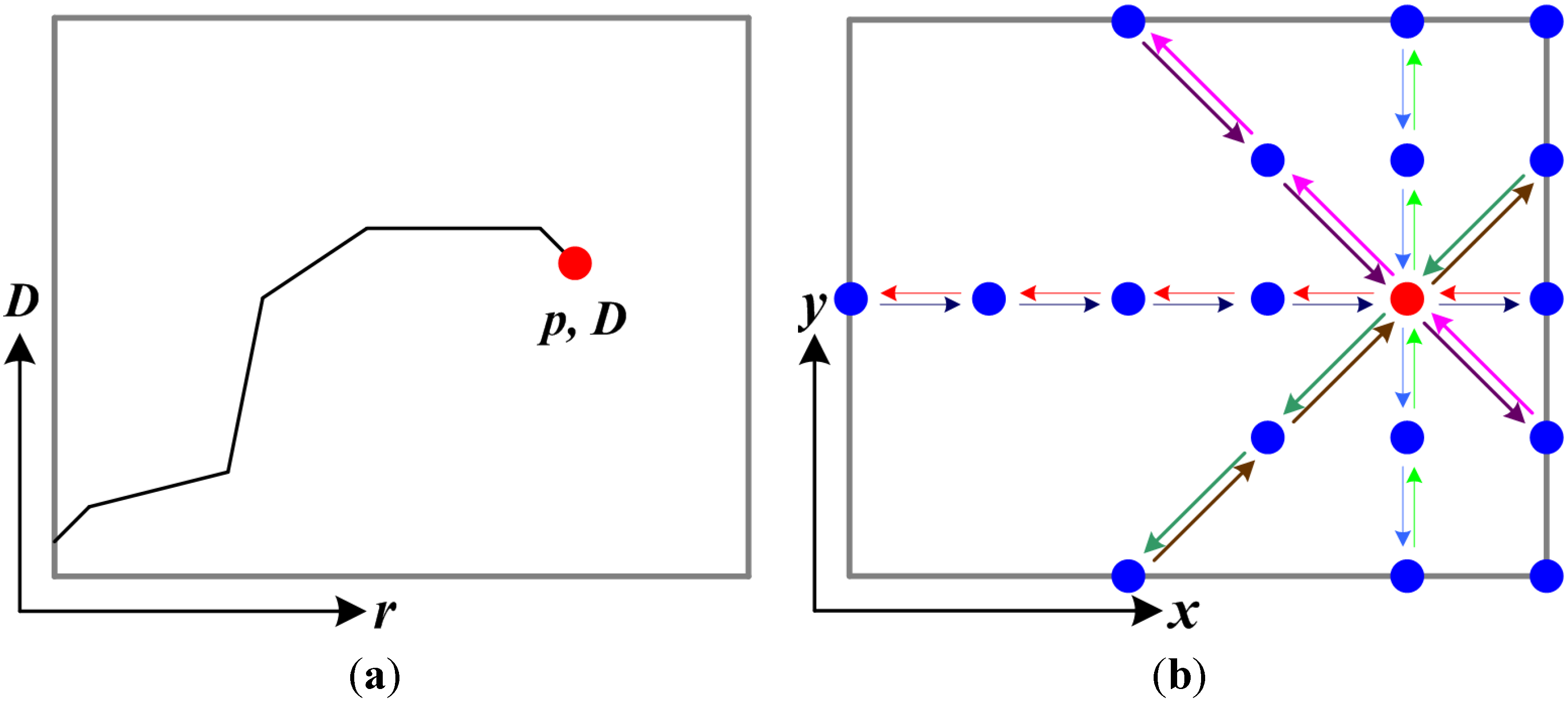
2.2. Computation of Ground Saliency for Adaptively Balancing the Energy Function


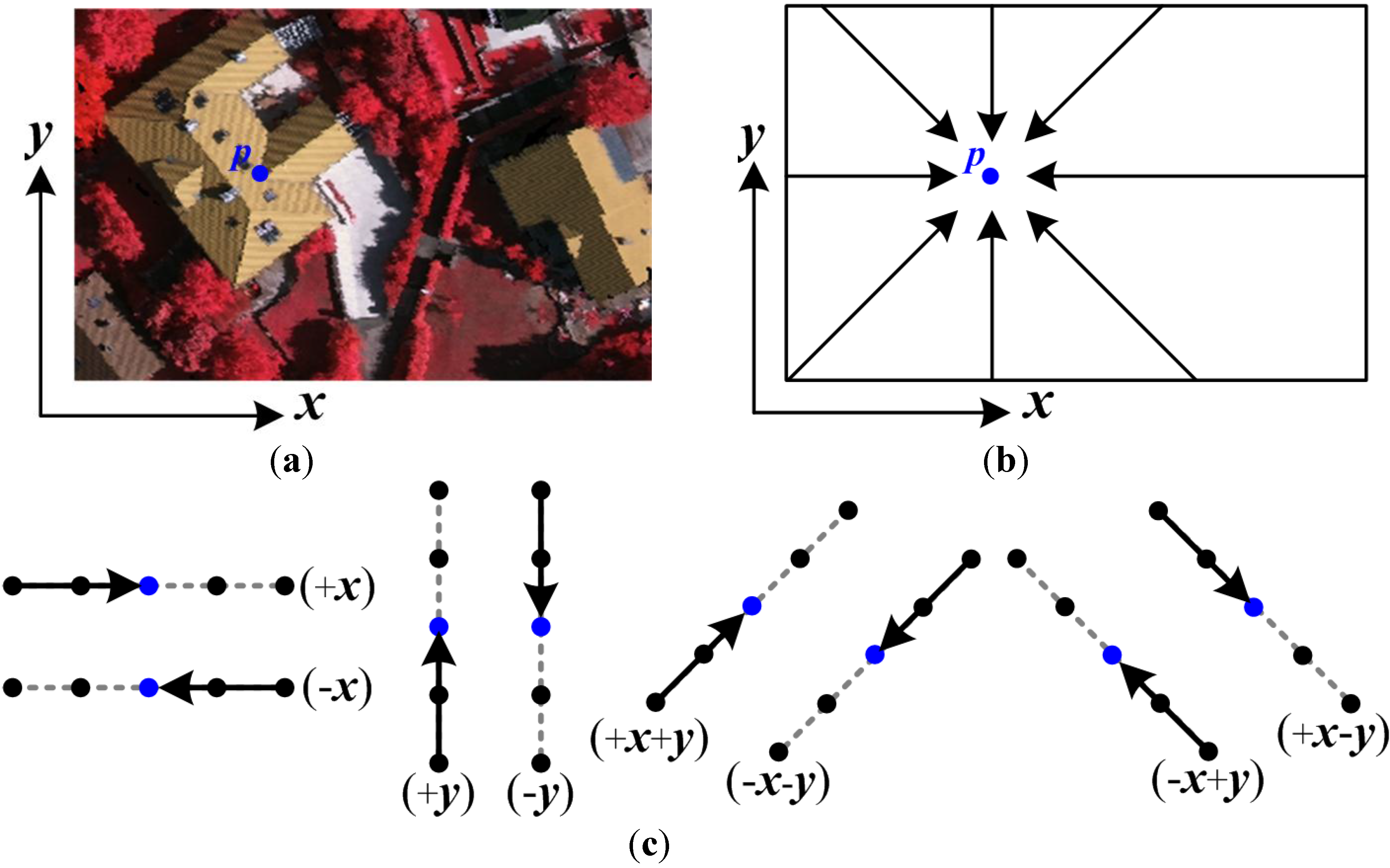
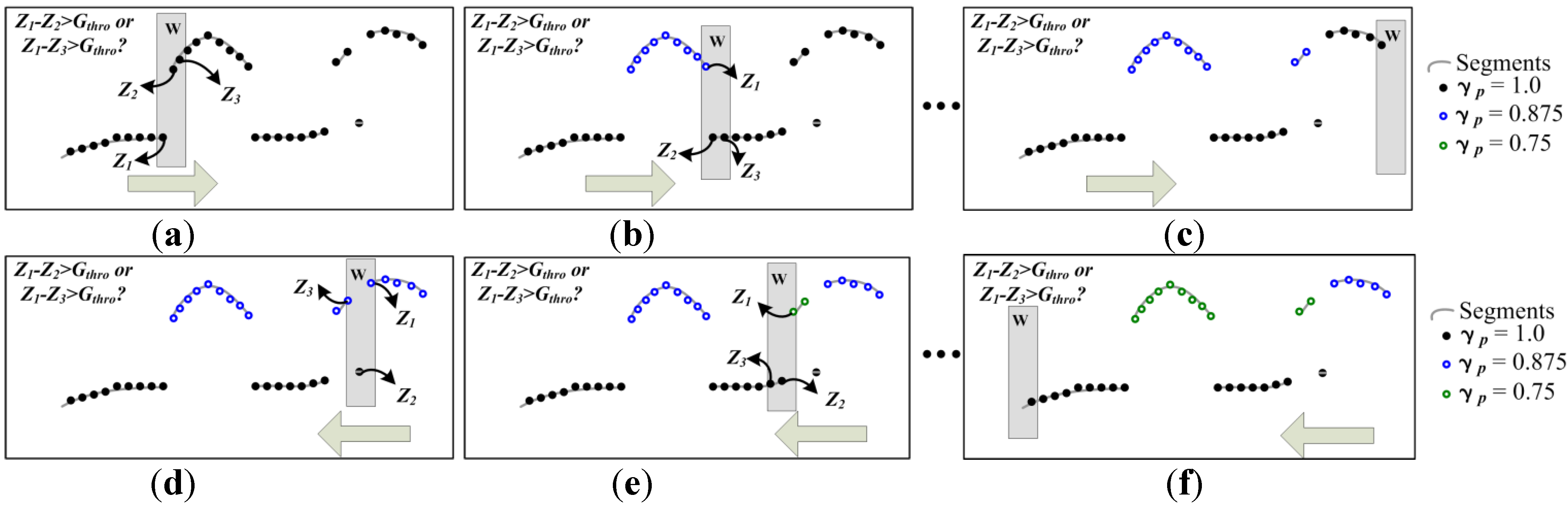
2.3. Semi-Global Optimization
2.3.1. Semi-Global Matching

2.3.2. Cost Aggregation of SGF

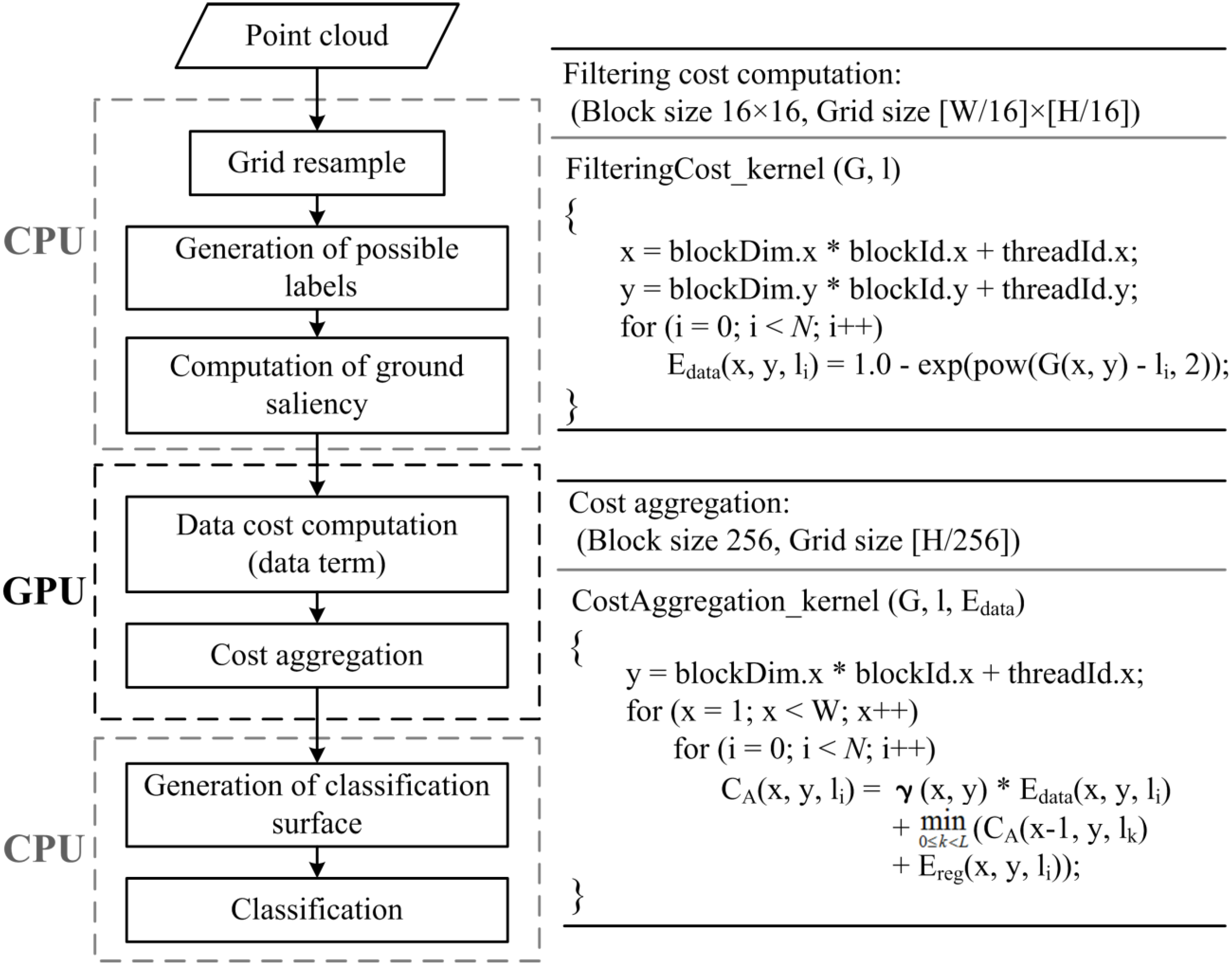
2.4. GPU Acceleration of SGF Algorithm

2.5. Point Filtering and Parameter Setting
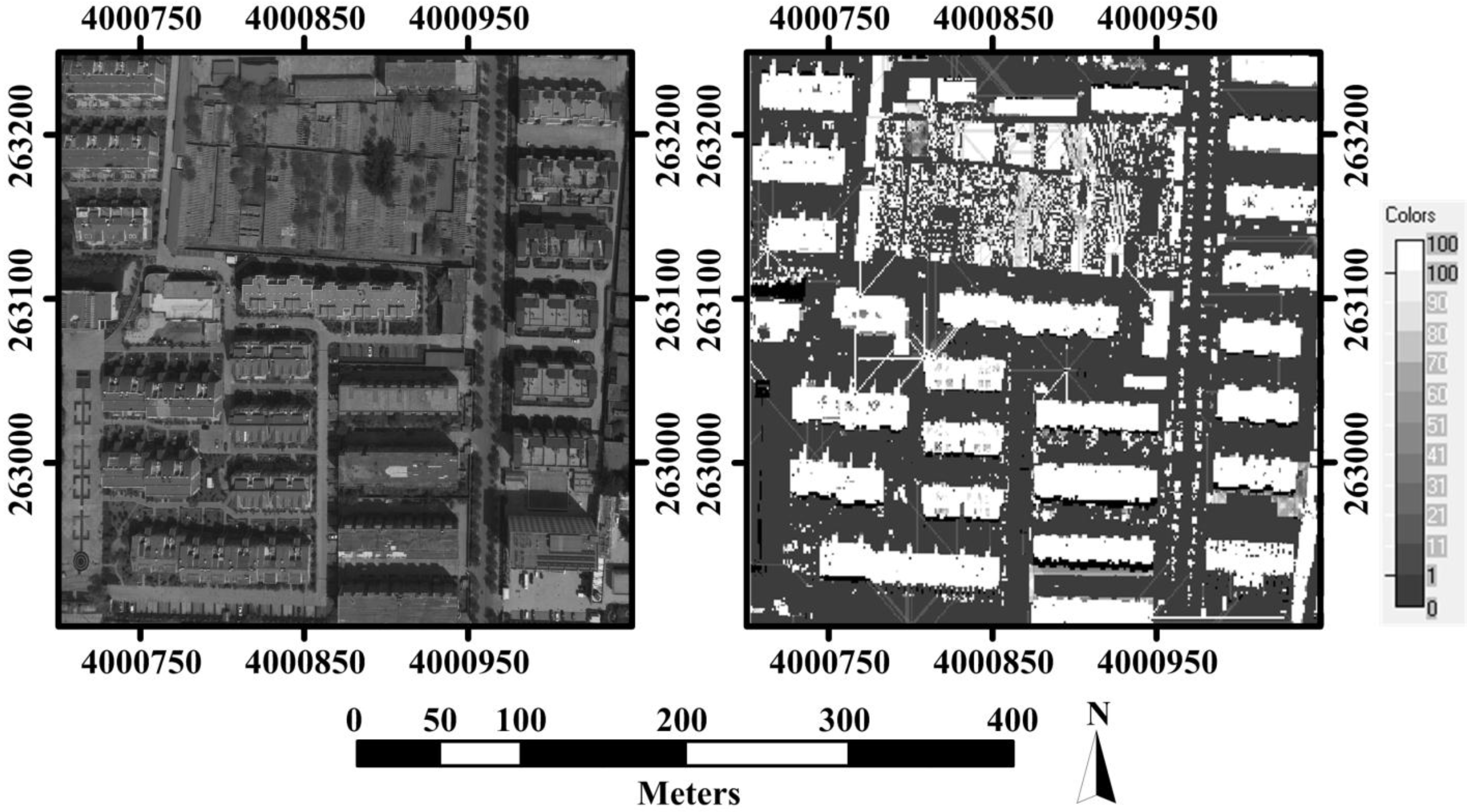
3. Experimental Results and Discussion
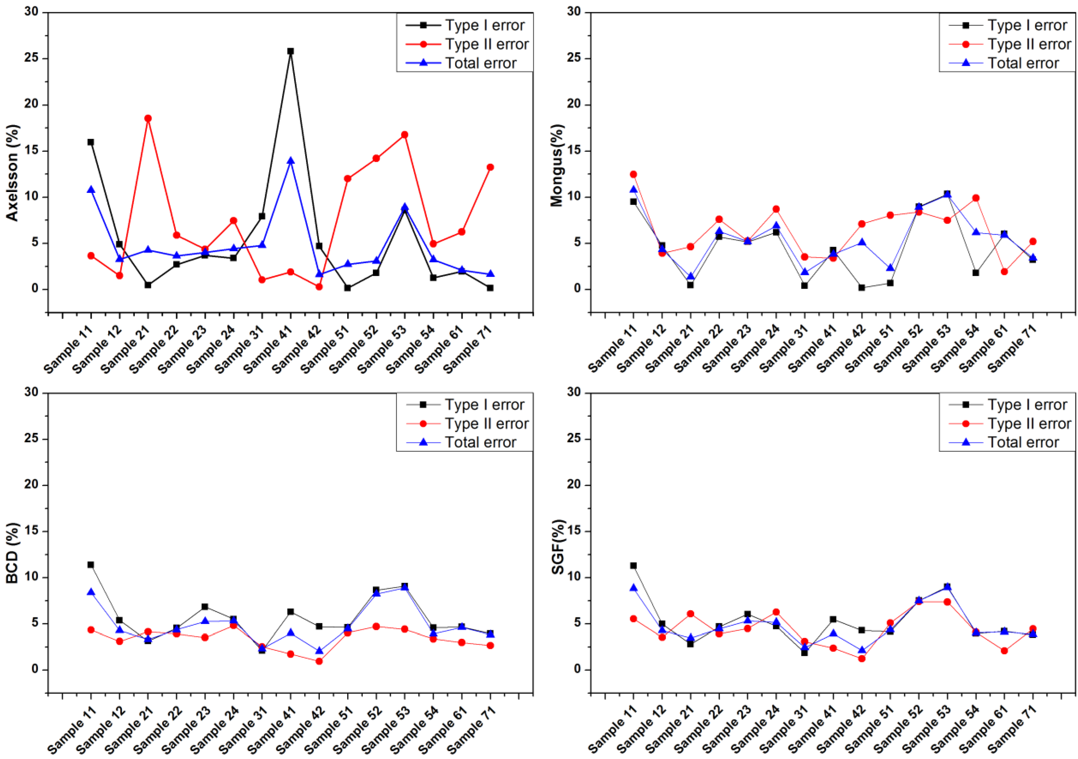
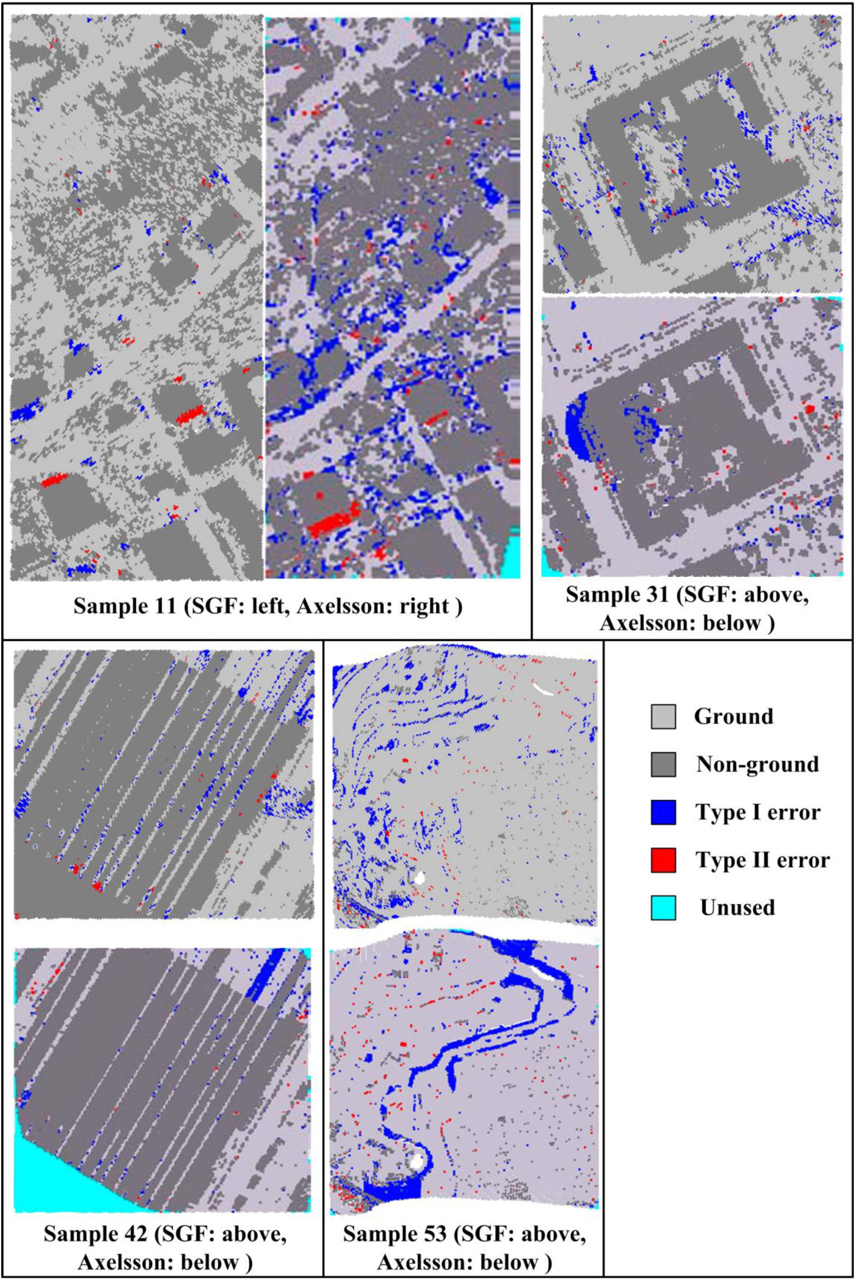
3.1. Quality Assessment on ISPRS Test Data Set

| Type I Error (%) | Type II Error (%) | Total Error (%) | |
|---|---|---|---|
| Elmqvist | 39.43 | 1.96 | 20.73 |
| Sohn | 9.94 | 8.59 | 9.35 |
| Axelsson | 5.55 | 7.46 | 4.82 |
| Pfeifer | 10.82 | 3.32 | 8.02 |
| Brovelli | 36.77 | 1.88 | 25.78 |
| Roggero | 17.12 | 3.11 | 12.35 |
| Wack | 16.52 | 1.58 | 12.04 |
| Sithole | 24.59 | 2.08 | 17.48 |
| Mongus | 4.5 | 6.5 | 5.49 |
| TerraScan | 11.05 | 4.52 | 7.61 |
| BCD | 5.69 | 3.41 | 4.88 |
| SGF | 5.25 | 4.46 | 4.85 |


3.2. Computational Performance
| Test Dataset | Sample | Sample1 | Sample2 | Sample3 | Sample4 | Sample5 |
|---|---|---|---|---|---|---|
| Number of Points (million) | 5.4 | 10.3 | 24.3 | 40.2 | 48.6 | |
| TerraScan | CPU (s) | 15.1 | 31.4 | 75.8 | 115.4 | 140.3 |
| GPU (s) | * | * | * | * | * | |
| BCD | CPU (s) | 28.24 | 60.53 | 148.69 | 224.85 | 278.91 |
| GPU (s) | 5.32 | 9.25 | 22.47 | 32.54 | 41.61 | |
| SGF | CPU (s) | 9.67 | 19.21 | 44.54 | 75.38 | 89.62 |
| GPU (s) | 1.91 | 3.52 | 8.11 | 12.36 | 15.42 |
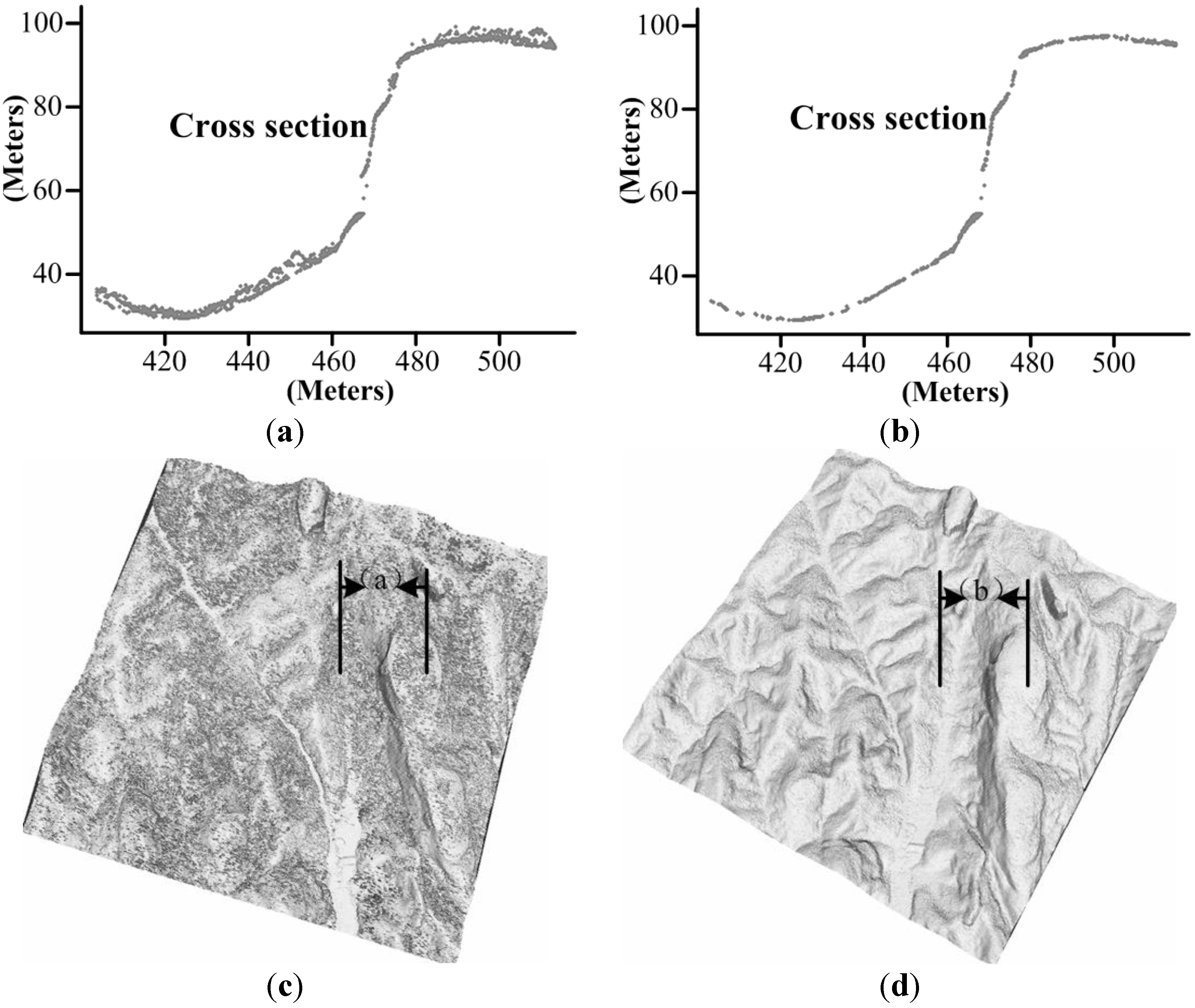
3.3. Discussion


4. Conclusions
Acknowledgments
Author Contributions
Conflicts of Interest
References
- Mongus, D.; Žalik, B. Parameter-free ground filtering of LiDAR data for automatic DTM generation. ISPRS J. Photogramm. Remote Sens. 2012, 67, 1–12. [Google Scholar] [CrossRef]
- Sithole, G.; Vosselman, G. Experimental comparison of filter algorithms for bare-Earth extraction from airborne laser scanning point clouds. ISPRS J. Photogramm. Remote Sens. 2004, 59, 85–101. [Google Scholar] [CrossRef]
- Liu, X. Airborne LiDAR for DEM generation: some critical issues. Prog. Phys. Geog. 2008, 32, 31–49. [Google Scholar]
- Vosselman, G. Slope based filtering of laser altimetry data. Int. Arch. Photogramm. Remote Sens. 2000, 33, 935–942. [Google Scholar]
- Shan, J.; Aparajithan, S. Urban DEM generation from raw LiDAR data. Photogramm. Eng. Remote Sens. 2005, 71, 217–226. [Google Scholar] [CrossRef]
- Meng, X.; Wang, L.; Silván-Cárdenas, J.L.; Currit, N. A multi-directional ground filtering algorithm for airborne LiDAR. ISPRS J. Photogramm. Remote Sens. 2009, 64, 117–124. [Google Scholar] [CrossRef]
- Susaki, J. Adaptive slope filtering of airborne LiDAR data in urban areas for digital terrain model (DTM) generation. Remote Sens. 2012, 4, 1804–1819. [Google Scholar] [CrossRef] [Green Version]
- Kraus, K.; Pfeifer, N. Determination of terrain models in wooded areas with airborne laser scanner data. ISPRS J. Photogramm. Remote Sens. 1998, 53, 193–203. [Google Scholar] [CrossRef]
- Pfeifer, N.; Reiter, T.; Briese, C.; Rieger, W. Interpolation of high quality ground models from laser scanner data in forested areas. Int. Arch. Photogramm. Remote Sens. 1999, 32, 31–36. [Google Scholar]
- Lee, H.S.; Younan, N.H. DTM extraction of LiDAR returns via adaptive processing. IEEE Trans. Geosci. Remote Sens. 2003, 41, 2063–2069. [Google Scholar] [CrossRef]
- Zhang, K.; Chen, S.; Whitman, D.; Shyu, M.; Yan, J.; Zhang, C. A progressive morphological filter for removing nonground measurements from airborne LiDAR data. IEEE Trans. Geosci. Remote Sens. 2003, 41, 872–882. [Google Scholar] [CrossRef]
- Chen, Q.; Gong, P.; Baldocchi, D.; Xie, G. Filtering airborne laser scanning data with morphological methods. Photogramm. Eng. Remote Sens. 2007, 73, 175–185. [Google Scholar] [CrossRef]
- Mongus, D.; Lukač, N.; Žalik, B. Ground and building extraction from LiDAR data based on differential morphological profiles and locally fitted surfaces. ISPRS J. Photogramm. Remote Sens. 2014, 93, 145–156. [Google Scholar] [CrossRef]
- Axelsson, P. DEM generation from laser scanner data using adaptive TIN models. Int. Arch. Photogramm. Remote Sens. 2000, 33, 111–118. [Google Scholar]
- Sohn, G.; Dowman, I.J. Terrain surface reconstruction by the use of tetrahedron model with the MDL criterion. Int. Arch. Photogramm. Remote Sens. 2002, 34, 336–344. [Google Scholar]
- Kang, X.; Liu, J.; Lin, X. Streaming progressive TIN densification filter for airborne LiDAR point clouds using multi-core architectures. Remote Sens. 2014, 6, 7212–7232. [Google Scholar] [CrossRef]
- Sithole, G.; Vosselman, G. Filtering of airborne laser scanner data based on segmented point clouds. Int. Arch. Photogramm. Remote Sens. 2005, 36, 66–71. [Google Scholar]
- Tóvári, D.; Pfeifer, N. Segmentation based robust interpolation-a new approach to laser data filtering. In Proceedings of the ISPRS Workshop Laser scanning 2005, Enschede, The Netherlands, 12–14 September 2005.
- Tolt, G.; Persson, Å.; Landgård, J.; Söderman, U. Segmentation and classification of airborne laser scanner data for ground and building detection. In Proceedings of the Defense and Security Symposium, Orlando, FL, USA, 17 April 2006.
- Meng, X.; Currit, N.; Zhao, K. Ground filtering algorithms for airborne LiDAR data: A review of critical issues. Remote Sens. 2010, 2, 833–860. [Google Scholar] [CrossRef]
- Elmqvist, M. Ground surface estimation from airborne laser scanner data using active shape models. Int. Arch. Photogramm. Remote Sens. 2002, 34, 114–118. [Google Scholar]
- Zhou, Q.; Neumann, U. Complete residential urban area reconstruction from dense aerial LiDAR point clouds. Graph. Models 2013, 75, 118–125. [Google Scholar] [CrossRef]
- Verdie, Y.; Lafarge, F.; Alliez, P. LOD Generation for urban scenes. Acm. Trans. Graph. 2015, 34, 15–29. [Google Scholar] [CrossRef]
- Chen, Q.; Koltun, V. Fast MRF optimization with application to depth reconstruction. In Proceedings of the Computer Vision and Pattern Recognition (CVPR), Columbus, OH, USA, 23–28 June 2014.
- Hirschmuller, H. Stereo Processing by semiglobal matching and mutual information. IEEE Trans. Pattern Anal. 2008, 30, 328–341. [Google Scholar] [CrossRef] [PubMed]
- Szeliski, R.; Zabih, R.; Scharstein, D.; Veksler, O.; Kolmogorov, V.; Agarwala, A.; Tappen, M.; Rother, C. A comparative study of energy minimization methods for markov random fields with smoothness-based priors. IEEE Trans. Pattern Anal. 2008, 30, 1068–1080. [Google Scholar] [CrossRef] [PubMed]
- Hu, X.; Li, X.; Zhang, Y. Fast filtering of LiDAR point cloud in urban areas based on scan line segmentation and GPU acceleration. IEEE Geosci. Remote Sens. 2013, 10, 308–312. [Google Scholar]
- Hirschmuller, H. Accurate and efficient stereo processing by semi-global matching and mutual information. In Proceedings of the Computer Vision and Pattern Recognition (CVPR), San Diego, CA, USA, 20–25 June 2005.
- Boykov, Y.; Veksler, O.; Zabih, R. Fast approximate energy minimization via graph cuts. IEEE Trans. Pattern Anal. Mach. Intell. 2001, 23, 1222–1239. [Google Scholar] [CrossRef]
- Hirschmuller, H. Semi-Global Matching-Motivation, Developments and Applications. Available online: http://hgpu.org/?p=6161 (accessed on 8 May 2015).
- Gehrke, S.; Morin, K.; Downey, M.; Boehrer, N.; Fuchs, T. Semi-global matching: An alternative to LiDAR for DSM generation. In Proceedings of the Canadian Geomatics Conference 2010 and ISPRS Com I Symposium, Calgary, AB, Canada, 15–18 June 2010.
- Drory, A.; Haubold, C.; Avidan, S.; Hamprecht, F.A. Semi-global matching: A principled derivation in terms of message passing. In Pattern Recognition; Springer International Publishing: Cham, Switzerland, 2014; pp. 43–53. [Google Scholar]
- Birchfield, S.; Tomasi, C. Depth discontinuities by pixel-to-pixel stereo. Int. J. Comput. Vision 1999, 35, 269–293. [Google Scholar] [CrossRef]
- Van Meerbergen, G.; Vergauwen, M.; Pollefeys, M.; van Gool, L. A hierarchical symmetric stereo algorithm using dynamic programming. Int. J. Comput. Vis. 2002, 47, 275–285. [Google Scholar] [CrossRef]
- Kolmogorov, V.; Zabih, R. Computing visual correspondence with occlusions using graph cuts. In Proceedings of the Eighth International Conference on Computer Vision, Vancouver, BC, Canada, 7–14 July 2001.
- Klaus, A.; Sormann, M.; Karner, K. Segment-based stereo matching using belief propagation and a self-adapting dissimilarity measure. In Proceedings of the 18th International Conference on Pattern Recognition (ICPR 2006), Hong Kong, China, 20–24 August 2006.
- Yang, Q.; Wang, L.; Yang, R.; Stewénius, H.; Nistér, D. Stereo matching with color-weighted correlation, hierarchical belief propagation, and occlusion handling. IEEE T. Pattern Anal. 2009, 31, 492–504. [Google Scholar] [CrossRef] [PubMed]
- Sun, J.; Li, Y.; Kang, S.B.; Shum, H. Symmetric stereo matching for occlusion handling. In Proceedings of the Computer Vision and Pattern Recognition (CVPR 2005), San Diego, CA, USA, 20–25 June 2005.
- Bleyer, M.; Gelautz, M. A layered stereo matching algorithm using image segmentation and global visibility constraints. ISPRS J. Photogramm. Remote Sens. 2005, 59, 128–150. [Google Scholar] [CrossRef]
- Haller, I.; Nedevschi, S. GPU optimization of the SGM stereo algorithm. In Proceedings of the Intelligent Computer Communication and Processing (ICCP), Cluj-Napoca, Romania, 26–28 August 2010.
- Nvidia, N. CUDA Toolkit Documentation v7.0. Available online: http://developer.download.nvidia.com/compute/cuda/3_2_prod/toolkit/docs/CUDA_C_Programming_Guide.pdf (accessed on 8 May 2015).
- Mongus, D.; Zalik, B. Computationally efficient method for the generation of a digital terrain model from airborne LiDAR data using connected operators. IEEE J. Sel. Top. App. Remote Sens. 2014, 7, 340–351. [Google Scholar] [CrossRef]
© 2015 by the authors; licensee MDPI, Basel, Switzerland. This article is an open access article distributed under the terms and conditions of the Creative Commons Attribution license (http://creativecommons.org/licenses/by/4.0/).
Share and Cite
Hu, X.; Ye, L.; Pang, S.; Shan, J. Semi-Global Filtering of Airborne LiDAR Data for Fast Extraction of Digital Terrain Models. Remote Sens. 2015, 7, 10996-11015. https://0-doi-org.brum.beds.ac.uk/10.3390/rs70810996
Hu X, Ye L, Pang S, Shan J. Semi-Global Filtering of Airborne LiDAR Data for Fast Extraction of Digital Terrain Models. Remote Sensing. 2015; 7(8):10996-11015. https://0-doi-org.brum.beds.ac.uk/10.3390/rs70810996
Chicago/Turabian StyleHu, Xiangyun, Lizhi Ye, Shiyan Pang, and Jie Shan. 2015. "Semi-Global Filtering of Airborne LiDAR Data for Fast Extraction of Digital Terrain Models" Remote Sensing 7, no. 8: 10996-11015. https://0-doi-org.brum.beds.ac.uk/10.3390/rs70810996