
Evaluation of Medium Spatial Resolution BRDF-Adjustment Techniques Using Multi-Angular SPOT4 (Take5) Acquisitions

 ,
,
Abstract
:
1. Introduction
2. The VJB BRDF Method
3. Data


| Sites | View Angles From East Satellite Track | View Angles from West Satellite Track | ||
|---|---|---|---|---|
| Zenith Range | Main Azimuth | Zenith Range | Main Azimuth | |
| Maricopa | (1.4, 8.7) | −105.9 | (21.9, 28.0) | 73.9 |
| ProvLanguedoc (overlap area) | (24.7, 25.3) | −109.6 | (0.2, 0.9) | 70.4 |
| Sudmipy (overlap area) | (12.2,12.6) | −109.7 | (12.8, 14.2) | 70.0 |

4. Methodology
4.1. Coarse Resolution Processing and BRDF Derivation
4.2. Land Cover Classification
4.3. High Resolution BRDF-Adjustment Techniques
| Techniques (short Name) | Reference | BRDF Approach | BRDF Dynamic | Use of Medium Resolution NDVI for Retrieving the BRDF | Use of Moderate Resolution BRDF | Use of Land-Cover Classification |
|---|---|---|---|---|---|---|
| Cst | - | VJB [6] | No BRDF dynamic | No | No | No |
| Av | [18] | Temporal variation with NDVI | Yes | |||
| VI-dis | - | Spatial and temporal variations | MODIS VJB coefficients (aggregated at 1250 m) | |||
| LC-dis | [12] | No | Yes (unsupervised classification) | |||
| LUM | [14] | MCD43 [2] | MODIS (MCD43 at 500 m) | Yes (CDL [32]) |
4.3.1. The Average Technique (Av)
4.3.2. The Land-Cover-Based Disaggregation Technique (LC-dis)
4.3.3. The Constant Technique (Cst)

4.3.4. The NDVI-Based Disaggregation Technique (VI-dis)
4.3.5. The Look-Up-Maps Technique (LUM)
4.4. The Evaluation Method
5. Results
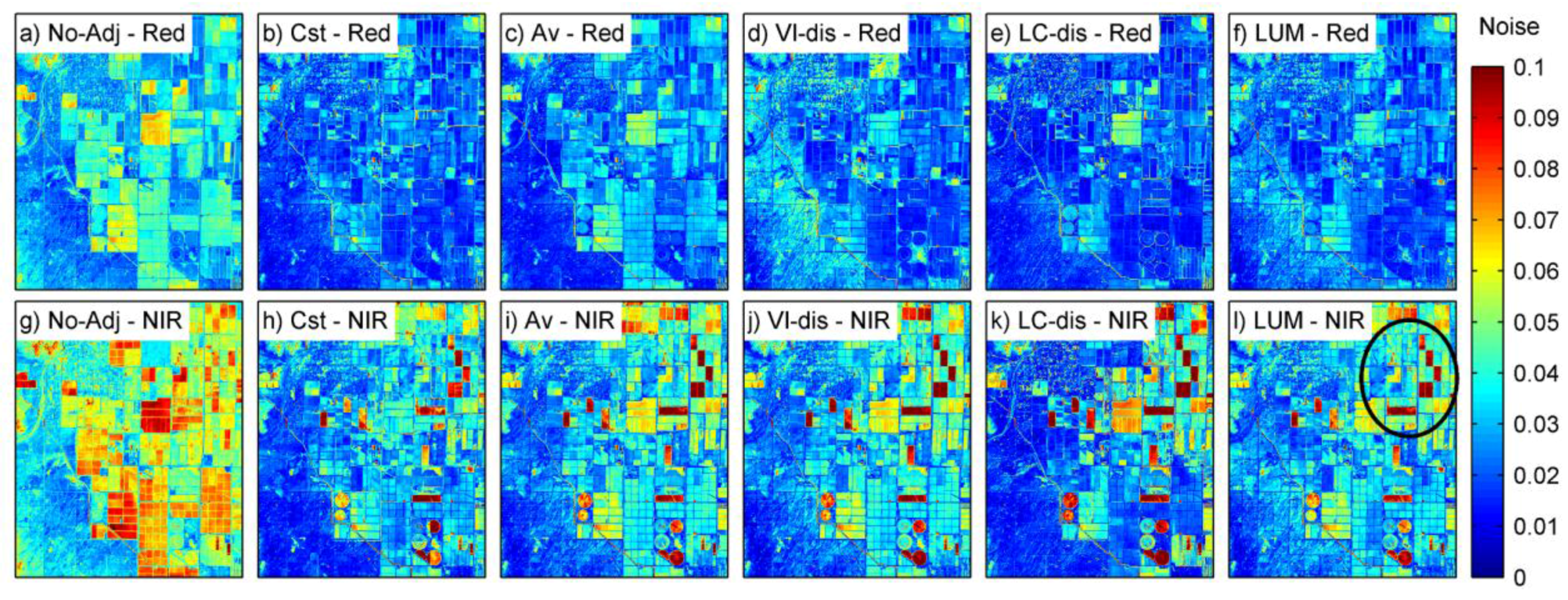
5.1. Maricopa Site


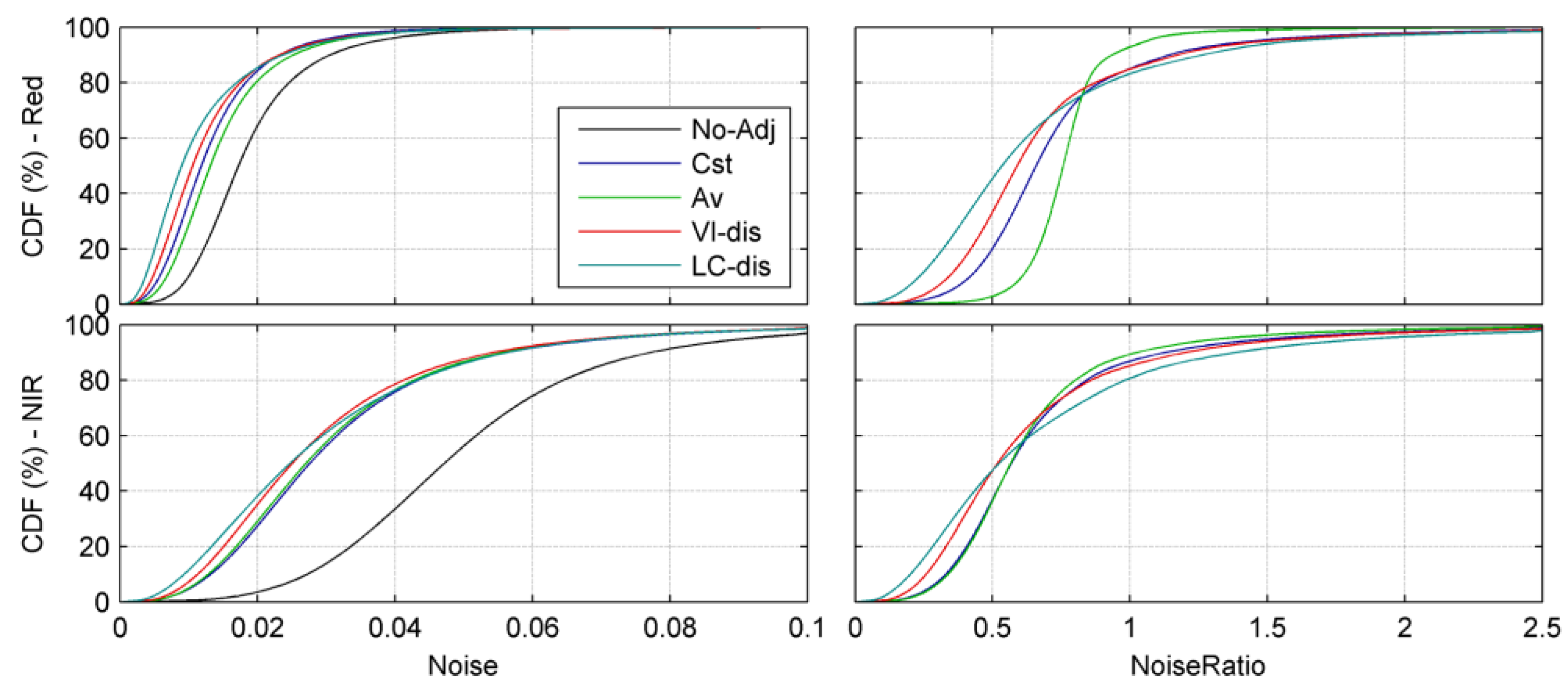
5.2. ProvLanguedoc and SudMipy Sites


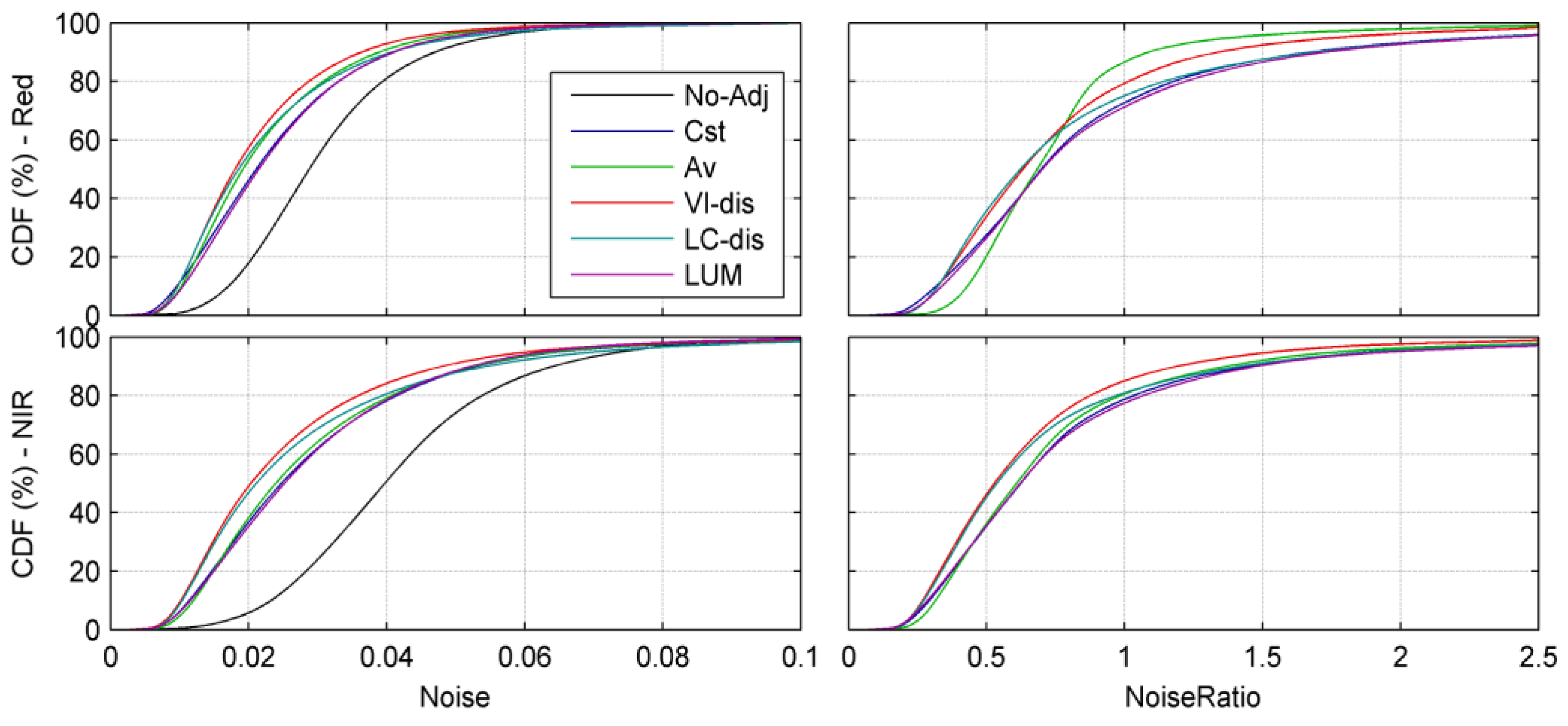
5.3. Overall Results

6. Conclusions
- The constant technique (Cst), which considers a uniform BRDF shape for all surfaces;
- The average technique (Av) which supposes the BRDF should shape vary uniformly for all surfaces with NDVI variations;
- The NDVI-based disaggregation technique (VI-dis) based on the disaggregation BRDF coefficient of the Vermote Justice Bréon (VJB) model using NDVI;
- The Land-cover-based disaggregation technique (LC-dis) based on the disaggregation of the MODIS BRDF coefficients of the VJB model using Land-cover; and
- The LUM technique (LUM) based on BRDF coefficients of the MCD43 products and using the US crop data layer.
Acknowledgments
Author Contributions
Conflicts of Interest
References
- Breon, F.M.; Maignan, F.; Leroy, M.; Grant, I. Analysis of hot spot directional signatures measured from space. J. Geophys. Res.-Atmos. 2002, 107, 4282–4296. [Google Scholar] [CrossRef]
- Lucht, W.; Schaaf, C.B.; Strahler, A.H. An algorithm for the retrieval of albedo from space using semiempirical BRDF models. IEEE Trans. Geosci. Remote Sens. 2000, 38, 977–998. [Google Scholar] [CrossRef]
- Schaaf, C.B.; Gao, F.; Strahler, A.H.; Lucht, W.; Li, X.W.; Tsang, T.; Strugnell, N.C.; Zhang, X.Y.; Jin, Y.F.; Muller, J.P.; et al. First operational BRDF, albedo nadir reflectance products from MODIS. Remote Sens. Environ. 2002, 83, 135–148. [Google Scholar] [CrossRef]
- Martonchik, J.V.; Diner, D.J.; Kahn, R.A.; Ackerman, T.P.; Verstraete, M.E.; Pinty, B.; Gordon, H.R. Techniques for the retrieval of aerosol properties over land and ocean using multiangle imaging. IEEE Trans. Geosci. Remote Sens. 1998, 36, 1212–1227. [Google Scholar] [CrossRef]
- Bacour, C.; Breon, F.M. Variability of biome reflectance directional signatures as seen by polder. Remote Sens. Environ. 2005, 98, 80–95. [Google Scholar] [CrossRef]
- Vermote, E.; Justice, C.O.; Breon, F.-M. Towards a generalized approach for correction of the BRDF effect in MODIS directional reflectances. IEEE Trans. Geosci. Remote Sens. 2009, 47, 898–908. [Google Scholar] [CrossRef]
- Drusch, M.; Del Bello, U.; Carlier, S.; Colin, O.; Fernandez, V.; Gascon, F.; Hoersch, B.; Isola, C.; Laberinti, P.; Martimort, P.; et al. Sentinel-2: ESA’s optical high-resolution mission for GMES operational services. Remote Sens. Environ. 2012, 120, 25–36. [Google Scholar] [CrossRef]
- Vermote, E.; Claverie, M.; Masek, J.; Becker-Reshef, I.; Justice, C. A merged surface reflectance product from the Landsat and Sentinel-2 missions. AGU Fall Meet. Abstr. 2013, 1, 0425. [Google Scholar]
- Roy, D.P.; Ju, J.; Lewis, P.; Schaaf, C.; Gao, F.; Hansen, M.; Lindquist, E. Multi-temporal MODIS-Landsat data fusion for relative radiometric normalization, gap filling, and prediction of Landsat data. Remote Sens. Environ. 2008, 112, 3112–3130. [Google Scholar] [CrossRef]
- Li, F.; Jupp, D.L.B.; Reddy, S.; Lymburner, L.; Mueller, N.; Tan, P.; Islam, A. An evaluation of the use of atmospheric and BRDF correction to standardize Landsat data. IEEE J. Sel. Top. Appl. Earth Obs. Remote Sens. 2010, 3, 257–270. [Google Scholar] [CrossRef]
- Shuai, Y.; Masek, J.G.; Gao, F.; Schaaf, C.B. An algorithm for the retrieval of 30-m snow-free albedo from Landsat surface reflectance and MODIS BRDF. Remote Sens. Environ. 2011, 115, 2204–2216. [Google Scholar] [CrossRef]
- Franch, B.; Vermote, E.F.; Claverie, M. Intercomparison of Landsat albedo retrieval techniques and evaluation against in situ measurements across the USA surfrad network. Remote Sens. Environ. 2014, 152, 627–637. [Google Scholar] [CrossRef]
- Jiao, Z.; Hill, M.J.; Schaaf, C.B.; Zhang, H.; Wang, Z.; Li, X. An anisotropic flat index (AFX) to derive BRDF archetypes from MODIS. Remote Sens. Environ. 2014, 141, 168–187. [Google Scholar] [CrossRef]
- Gao, F.; He, T.; Masek, J.G.; Shuai, Y.; Schaaf, C.B.; Wang, Z. Angular effects and correction for medium resolution sensors to support crop monitoring. Sel. Top. IEEE J. Appl. Earth Obs. Remote Sens. 2014, 7, 4480–4489. [Google Scholar] [CrossRef]
- Roy, D.P.; Borak, J.S.; Devadiga, S.; Wolfe, R.E.; Zheng, M.; Descloitres, J. The MODIS land product quality assessment approach. Remote Sens. Environ. 2002, 83, 62–76. [Google Scholar] [CrossRef]
- Roman, M.O.; Gatebe, C.K.; Shuai, Y.; Wang, Z.; Gao, F.; Masek, J.G.; He, T.; Liang, S.; Schaaf, C.B. Use of in situ and airborne multiangle data to assess MODIS- and Landsat-based estimates of directional reflectance and albedo. IEEE Trans. Geosci. Remote Sens. 2013, 51, 1393–1404. [Google Scholar] [CrossRef]
- Liang, S. Narowband to broadband conversions of land surface albedo. I algorithms. Remote Sens. Environ. 2000, 76, 213–238. [Google Scholar] [CrossRef]
- Breon, F.-M.; Vermote, E. Correction of MODIS surface reflectance time series for BRDF effects. Remote Sens. Environ. 2012, 125, 1–9. [Google Scholar] [CrossRef]
- Pinter, P.J.; Jackson, R.D.; Moran, M.S. Bidirectional reflectance factors of agricultural targets—A comparison of ground-based, aircraft-based, and satellite-based observations. Remote Sens. Environ. 1990, 32, 215–228. [Google Scholar] [CrossRef]
- Hagolle, O.; Sylvander, S.; Huc, M.; Claverie, M.; Clesse, D.; Dechoz, C.; Lonjou, V.; Poulain, V. Spot4 (take5): Simulation of Sentinel-2 time series on 45 large sites. Remote Sens. 2015. submitted. [Google Scholar]
- Tan, B.; Woodcock, C.E.; Hu, J.; Zhang, P.; Ozdogan, M.; Huang, D.; Yang, W.; Knyazikhin, Y.; Myneni, R.B. The impact of gridding artifacts on the local spatial properties of MODIS data: Implications for validation, compositing, and band-to-band registration across resolutions. Remote Sens. Environ. 2006, 105, 98–114. [Google Scholar] [CrossRef]
- Franch, B.; Vermote, E.F.; Sobrino, J.A.; Julien, Y. Retrieval of surface albedo on a daily basis: Application to MODIS data. IEEE Trans. Geosci. Remote Sens. 2014, 52, 7549–7558. [Google Scholar] [CrossRef]
- Claverie, M.; Vermote, E.F.; Franch, B.; Masek, J.G. Evaluation of the Landsat-5 tm and Landsat-7 ETM+ surface reflectance products. Remote Sens. Environ. 2015, 169, 390–403. [Google Scholar]
- Claverie, M.; Vermote, E.F.; Weiss, M.; Baret, F.; Hagolle, O.; Demarez, V. Validation of coarse spatial resolution LAI and FAPAR time series over cropland in southwest France. Remote Sens. Environ. 2013, 139, 216–230. [Google Scholar] [CrossRef]
- De Abelleyra, D.; Verón, S.R. Comparison of different BRDF correction methods to generate daily normalized MODIS 250 m time series. Remote Sens. Environ. 2014, 140, 46–59. [Google Scholar] [CrossRef]
- Roujean, J.L.; Leroy, M.; Deschamps, P.Y. A bidirectional reflectance model of the earths surface for the correction of remote-sensing data. J. Geophys. Res.-Atmos. 1992, 97, 20455–20468. [Google Scholar] [CrossRef]
- Li, X.W.; Strahler, A.H. Geometric-optical bidirectional reflectance modeling of the discrete crown vegetation canopy—Effect of crown shape and mutual shadowing. IEEE Trans. Geosci. Remote Sens. 1992, 30, 276–292. [Google Scholar] [CrossRef]
- Lucht, W. Expected retrieval accuracies of bidirectional reflectance and albedo from Eos-MODIS and MISR angular sampling. J. Geophys. Res.-Atmos. 1998, 103, 8763–8778. [Google Scholar] [CrossRef]
- Campagnolo, M.L.; Montano, E.L. Estimation of effective resolution for daily MODIS gridded surface reflectance products. IEEE Trans. Geosci. Remote Sens. 2014, 52, 5622–5632. [Google Scholar] [CrossRef]
- Breon, F.; Vermote, E.; Murphy, E.; Franch, B. Measuring the directional variations of land surface reflectance from MODIS. IEEE Trans. Geosci. Remote Sens. 2015, 53, 4638–4649. [Google Scholar] [CrossRef]
- Wolfe, R.E.; Nishihama, M.; Fleig, A.J.; Kuyper, J.A.; Roy, D.P.; Storey, J.C.; Patt, F.S. Achieving sub-pixel geolocation accuracy in support of MODIS land science. Remote Sens. Environ. 2002, 83, 31–49. [Google Scholar] [CrossRef]
- USDA. National Agricultural Statistics Service (NASS) Cropland Data Layer (CDL). Available online: http://www.nass.usda.gov/research/Cropland/SARS1a.htm (accessed on 21 May 2015).
- Späth, H. Cluster Dissection and Analysis: Theory, FORTRAN Programs, Examples; Prentice-Hall, Inc: Upper Saddle River, NJ, USA, 1986. [Google Scholar]
- Hagolle, O.; Huc, M.; Villa Pascual, D.; Dedieu, G. A multi-temporal and multi-spectral method to estimate aerosol optical thickness over land, for the atmospheric correction of formosat-2, Landsat, venμs and Sentinel-2 images. Remote Sens. 2015, 7, 2668–2691. [Google Scholar] [CrossRef]
- Hagolle, O.; Dedieu, G.; Mougenot, B.; Debaecker, V.; Duchemin, B.; Meygret, A. Correction of aerosol effects on multi-temporal images acquired with constant viewing angles: Application to formosat-2 images. Remote Sens. Environ. 2008, 112, 1689–1701. [Google Scholar] [CrossRef] [Green Version]
- Comar, A.; Baret, F.; Vienot, F.; Yan, L.; de Solan, B. Wheat leaf bidirectional reflectance measurements: Description and quantification of the volume, specular and hot-spot scattering features. Remote Sens. Environ. 2012, 121, 26–35. [Google Scholar] [CrossRef]
© 2015 by the authors; licensee MDPI, Basel, Switzerland. This article is an open access article distributed under the terms and conditions of the Creative Commons Attribution license (http://creativecommons.org/licenses/by/4.0/).
Share and Cite
Claverie, M.; Vermote, E.; Franch, B.; He, T.; Hagolle, O.; Kadiri, M.; Masek, J. Evaluation of Medium Spatial Resolution BRDF-Adjustment Techniques Using Multi-Angular SPOT4 (Take5) Acquisitions. Remote Sens. 2015, 7, 12057-12075. https://0-doi-org.brum.beds.ac.uk/10.3390/rs70912057
Claverie M, Vermote E, Franch B, He T, Hagolle O, Kadiri M, Masek J. Evaluation of Medium Spatial Resolution BRDF-Adjustment Techniques Using Multi-Angular SPOT4 (Take5) Acquisitions. Remote Sensing. 2015; 7(9):12057-12075. https://0-doi-org.brum.beds.ac.uk/10.3390/rs70912057
Chicago/Turabian StyleClaverie, Martin, Eric Vermote, Belen Franch, Tao He, Olivier Hagolle, Mohamed Kadiri, and Jeff Masek. 2015. "Evaluation of Medium Spatial Resolution BRDF-Adjustment Techniques Using Multi-Angular SPOT4 (Take5) Acquisitions" Remote Sensing 7, no. 9: 12057-12075. https://0-doi-org.brum.beds.ac.uk/10.3390/rs70912057