Interannual Variability in Dry Mixed-Grass Prairie Yield: A Comparison of MODIS, SPOT, and Field Measurements

Abstract

Remote sensing is often used to assess rangeland condition and biophysical parameters across large areas. In particular, the relationship between the Normalized Difference Vegetation Index (NDVI) and above-ground biomass can be used to assess rangeland primary productivity (seasonal carbon gain or above-ground biomass “yield”). We evaluated the NDVI–yield relationship for a southern Alberta prairie rangeland, using seasonal trends in NDVI and biomass during the 2009 and 2010 growing seasons, two years with contrasting rainfall regimes. The study compared harvested biomass and NDVI from field spectrometry to NDVI from three satellite platforms: the Aqua and Terra Moderate Resolution Imaging Spectroradiometer (MODIS) and Système Pour l’Observation de la Terre (SPOT 4 and 5). Correlations between ground spectrometry and harvested biomass were also examined for each growing season. The contrasting precipitation patterns were easily captured with satellite NDVI, field NDVI and green biomass measurements. NDVI provided a proxy measure for green plant biomass, and was linearly related to the log of standing green biomass. NDVI phenology clearly detected the green biomass increase at the beginning of each growing season and the subsequent decrease in green biomass at the end of each growing season due to senescence. NDVI–biomass regressions evolved over each growing season due to end-of-season senescence and carryover of dead biomass to the following year. Consequently, mid-summer measurements yielded the strongest correlation (R² = 0.97) between NDVI and green biomass, particularly when the data were spatially aggregated to better match the satellite sampling scale. Of the three satellite platforms (MODIS Aqua, MODIS Terra, and SPOT), Terra yielded the best agreement with ground-measured NDVI, and SPOT yielded the weakest relationship. When used properly, NDVI from satellite remote sensing can accurately estimate peak-season productivity and detect interannual variation in standing green biomass, and field spectrometry can provide useful validation for satellite data in a biomass monitoring program in this prairie ecosystem. Together, these methods can be used to identify the effects of year-to-year precipitation variability on above-ground biomass in a dry mixed-grass prairie. These findings have clear applications in monitoring yield and productivity, and could be used to support a rangeland carbon monitoring program.

1. Introduction

Rangelands comprise between 26 to 36 percent of the terrestrial land surface [1,2]. They consist of many ecosystems, including shrublands, savannas, tundra, deserts, alpine communities, coastal marshes, meadows, and grasslands [3]. Historically, grasslands covered 300 million ha in the United States and 50 million ha in Canada [4]. The mixed prairie, one grassland type, is located in the brown and dark brown soil regions of southern Alberta and Saskatchewan, Canada, and extends southward into northern Texas [5]. Approximately 7 percent of the area of Alberta is covered by the dry mixed-grass prairie subregion, of which 43 percent remains [6]. Climate is the determining factor for production and health in this ecosystem [1,7,8], and water availability largely controls productivity [1,9,10]. Climate change is expected to increase the amount and duration of growing season drought, as well as alter the frequency and intensity of growing season precipitation [1,11]. Knapp and Smith [10] demonstrated that prairie ecosystems have high production potential and substantial interannual variability, and are likely to be one of the most responsive biomes to future climate change [10]. Human interest in these areas is usually focused on yearly productivity [12] or biomass yields for economic and ecological monitoring purposes. The most common land use in the mixed prairie is ranching, as much of it is too dry to accommodate crop production without irrigation. Consequently, the economy in these regions is dominated by livestock ranching and supporting businesses. An emerging interest in prairie regions is yield assessment for agricultural insurance, which for prairies is limited by the inability to produce a direct, measurable yield; unlike traditional agriculture, a harvested crop yield is not the end product [13]. Prairie vegetation functions to prevent soil erosion and resist landscape degradation, facilitate groundwater recharge, sequester large amounts of carbon dioxide, and support plant and animal diversity [14,15], which are often positively related to productivity [16,17]. Due to the potential for biospheric carbon sequestration and other co-benefits, in a period with deepening concerns about anthropogenically-induced climate change, there is also an emerging possibility of targeted carbon markets and economic incentives for proper land stewardship in these areas. These economic and ecological issues require accurate methods of evaluating prairie biomass yield in response to interannual variations in precipitation, especially given the current climate variability and predictions for future climate change.

Clearly, accurate monitoring methods are necessary for proper management of the mixed prairie. Traditionally, range management has been accomplished through the subjective evaluation and monitoring of large areas by skilled professionals relying on accumulated judgment and experience [18]. This methodology has limitations for widespread application. Quantitative estimates of prairie productivity have also often been conducted through biomass harvests, which are expensive and time-consuming [18,19,20,21]. Biomass harvests are destructive, so repeated sampling of a single plot is not possible, limiting the temporal practicality of the method. The time-consuming nature of manual field sampling, combined with the expansive size of these ecosystems, further limits the utility of biomass harvests for prairie management [19,20,21]. Harvests require measurements to be performed in a representative number of places during a short time period and extrapolated to useful spatial and temporal scales. This often entails measurement errors, inaccuracies inherent in interpolation techniques, and delays in evaluating results that impair effective management.

The requirement for a sampling method that limits error introduced by inadequate sample size and distribution often exacerbated by personal bias [18] has led to the exploration of remote sensing techniques for rangeland monitoring. Spectral reflectance enables non-destructive sampling over a wide range of spatial and temporal scales. Remote sensing data from multiple satellite platforms have been available since the 1970s [18]. Many publicly funded satellites monitor the Earth, including the NASA Terra and Aqua satellites, which carry the MODIS (Moderate Resolution Imaging Spectroradiometer) sensors. These satellite sensors provide 250 m spatial resolution from 36 spectral bands, with daily coverage [18,22]. MODIS products are created from quality-controlled multiband surface radiance and reflectance, and are freely available through websites developed by U.S. government agencies. The availability of quality-controlled satellite data has led to their widespread use and increased practicality for management and science.

Remote sensing data are also readily available for purchase from commercial satellite vendors. For example, the Système Pour l’Observation de la Terre SPOT 5 satellite produces 10 m spatial resolution multispectral imagery (SPOT 4 can also produce 10 m spatial resolution by co-registering a 10 m panchromatic and 20 m colour image) from four bands, two in the visible wavelengths, one in the near infrared and one in the shortwave infrared [23]. The increased spatial resolution limits the possible temporal resolution such that SPOT samples a position on the Earth every 26 days, although the sensor can be pointed off nadir at targets not directly below the satellite, increasing the temporal resolution [18]. Commercial satellites offer several potential advantages over MODIS; the finer spatial resolution of commercial satellites offer the potential of providing data products that more closely match the scales of small management units [24]. However, images from commercial systems are often prohibitively expensive for practical application for range management [18]. Commercial satellites also require tasking requests far in advance, and data gaps can occur with excessive cloud cover or otherwise reduced image quality during the tasking period [3]. Despite these limitations, private satellites represent alternatives to government-funded programs and are also being explored for rangeland monitoring.

Past studies have demonstrated the ability of remote sensing to accurately estimate plant biomass or yield in grasslands [18,20,25,26]. Satellite remote sensing also allows repetitive sampling, i.e., the creation of time series for evaluating growing season phenology and interannual variability in production. These methods enable productivity monitoring in near real time, relatively inexpensively, and with multiple scales of coverage. Many vegetation indices have been established from remotely sensed data. These indices provide proxies for vegetation biophysical properties, and can be used to diagnose rangeland conditions and trends [27,28]. The most commonly used vegetation index is the Normalized Difference Vegetation Index (NDVI) [21,29]. This index compares the low reflectance of photosynthetic materials in the red wavelengths to the high reflectance in the near-infrared to produce an estimation of plant biophysical parameters, including biomass, leaf area index (LAI) and the fraction of absorbed photosynthetically active radiation (f_APAR). Numerous studies have demonstrated that NDVI strongly correlates with green biomass and leaf area index, particularly for grassland ecosystems [19,25,26,30,31]. In grassland ecosystems, NDVI also provides a strong indicator of photosynthetic carbon uptake, typically measured via gas exchange or eddy covariance [16,26,31,32,33], indicating its potential as a useful metric for carbon sequestration. Furthermore, in prairies, NDVI often scales with metrics of species richness and evenness [16,17], so may also provide a useful indicator of biodiversity or other ecosystem co-benefits.

Due to the potential economic benefits of accurate prairie ecosystem monitoring, there is renewed commercial interest in evaluating cost-effective methods of assessing mixed prairie biomass. For example, the agricultural insurance industry has been exploring satellite remote-sensing-based monitoring programs and is interested in evaluating the accuracy of yield estimation in an effort to enhance customer confidence [34]. This interest influenced the goals of this research, which were to evaluate how effectively NDVI from different common satellite sensors can estimate spatial and interannual patterns of grassland yield, and how satellite measurements compare to biomass harvests and NDVI from ground measurement. A common practice in assessing the utility of remote sensing for rangeland management is to conduct studies over a single growing season, such that evaluation of the impacts of year-to-year variability in precipitation is limited [29]. Many other studies forego any intensive ground sampling with field spectrometers and rely only on data derived from broad-band satellite sensors [20], leaving issues of satellite validation unresolved. Furthermore, the lack of a single, universal NDVI formulation due to the many band and sampling configurations of existing satellite sensors requires independent calibrations be conducted. Satellite calibration and validation (“CalVal”) efforts have often focused on a limited number of core sites [35], and have been less concerned with evaluating the management applications of such sensors in the context of environmental change, leaving many aspects of validation to the scientific or end-user community. Consequently, there is an ongoing need to evaluate satellite sensors by comparing their output with field measurements, particularly when accurate data are needed for management regimes, carbon markets, or insurance purposes. Validation efforts comparing satellite measurements and traditional field sampling must, by definition, compare data collected on vastly different scales, necessitating some kind of scaling regime [36], adding to the challenges of quantitative yield estimates from satellites.

In this study we analyzed data from the SPOT, MODIS Terra and Aqua platforms, and ground spectrometry to calculate NDVI. We then compared the resulting NDVI values to harvested biomass from southern Albertan mixed-grass prairies over two consecutive summers (2009 and 2010) having contrasting rainfall regimes. The objectives of the study were to (1) determine whether NDVI time-series from satellite systems that are currently utilized for estimating productivity are comparable to measurements from a ground spectrometer and harvested biomass; (2) determine whether variations in productivity as a result of contrasting weather conditions over two consecutive summers are clearly detectable, which could indicate the utility of remote sensing for monitoring long-term or year-to-year climate variability in prairie systems; and (3) determine the practical utility of NDVI for estimating above-ground biomass (“yield”) in the mixed prairie. Addressing the last objective is an essential foundation for cost-effective satellite-based rangeland insurance or carbon management programs. Since accuracy is crucial for carbon markets and insurance programs, we also considered the relative performance of two satellite sensors, SPOT and MODIS (Aqua and Terra), using ground NDVI measurements as a reference.

2. Materials and Methods

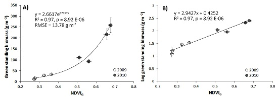
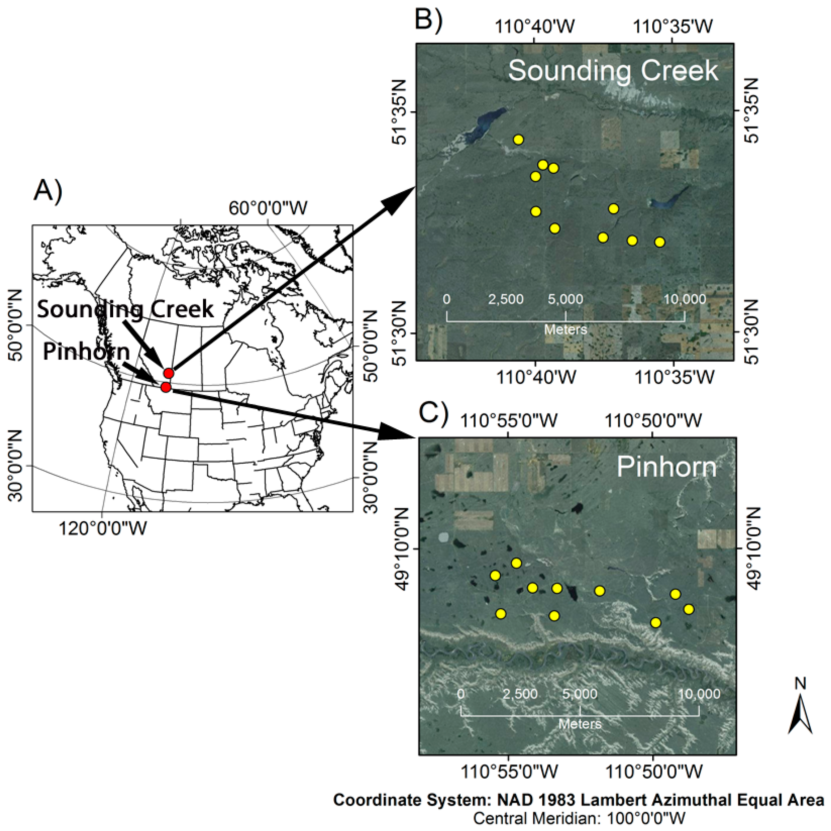
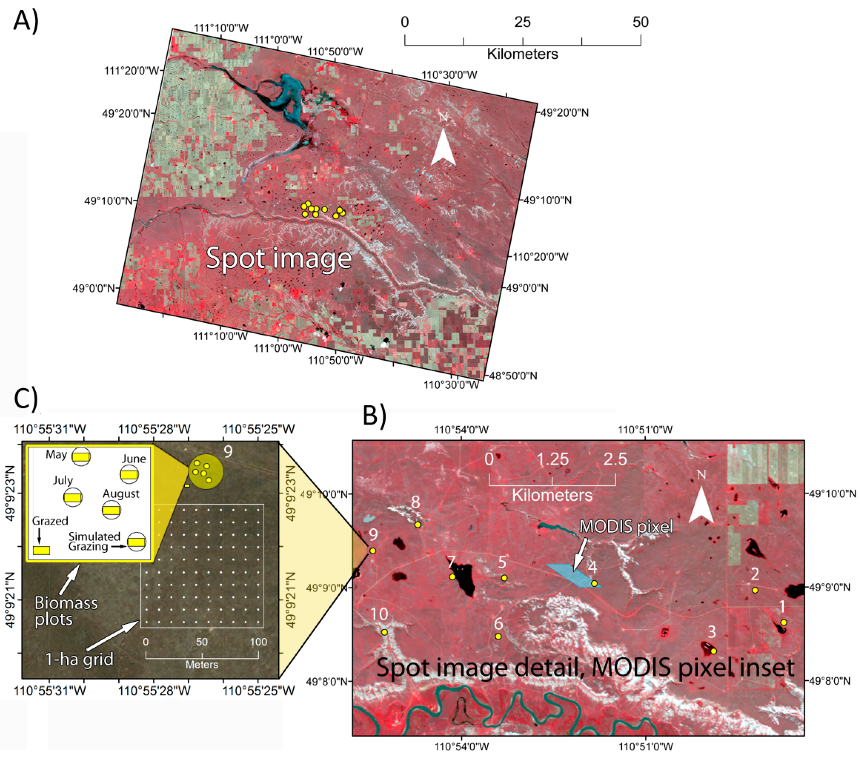
2.1. Study Location and Design

Field sites were located in the dry mixed-grass prairie ecoregion, within the Sounding Creek and Pinhorn Grazing Reserves, in southern Alberta, Canada (Figure 1). The Sounding Creek Grazing Reserve is located near the northern extent of the dry mixed-grass prairie, consequently it is dominated by the Stipa comata–Bouteloua gracilis range type. The Pinhorn Grazing Reserve is dominated by Bouteloua gracilis with some Stipa comata and Agropyron species due to differing edaphic conditions. Management regimes consisted of light, rotational grazing typical of the region (e.g., [31]). Average annual precipitation in these areas is around 325 mm per year [8]. The field data were collected in the summers of 2009 and 2010 in representative areas within the Grazing Reserves. These data were collected from randomly selected sites, located within similar range types and with a density of no more than one site per section (one square mile, or approximately 260 ha). This design created several site replicates at the township level, which allowed us to examine data at several spatial scales, ranging from single plots (1 m²) to whole townships (approx. 93 km²). The data shown in this study were aggregated to the township level by treatment for each month.

2.2. Plot Selection and Sample Design

At each sampling location, three (2009) or four (2010) plots were selected for harvesting, all located within grassland communities (i.e., sites with shrubs or trees were avoided). Within a location, these plots were in close proximity (several meters) to each other, matching vegetation types and landscape positions. To evaluate possible artifacts due to grazing, sample plots consisted of a 1-m diameter grazing exclosure, comprised of a modified wire mesh tree basket secured to the ground with rebar. Each site also had a matching, grazed control plot, which consisted of a similarly-sized sampling plot without an exclosure, located 10 m from a caged plot, and sampled in a different cardinal direction each month (to avoid repeatedly sampling the same location). Preliminary analysis indicated that, due to the light grazing regime, there was no significant difference between the grazed and ungrazed plot results, so these data were combined in the final analyses.

2.3. Biomass Harvests

Plots were sampled on a monthly basis during the growing season (May, June, July, and August; Figure 2), except that the May date was not sampled in 2009. Field sampling dates in 2009 were 10 and 11 June, 18 July, and 14 August for Sounding Creek; and 13 and 14 June, 15 and 16 July, and 11 August for Pinhorn. Field sampling dates in 2010 were 14 and 15 May, 23 and 24 June, 18 July, and 19 and 25 August for Sounding Creek; and 12 and 13 May, 25 and 26 June, 16 and 17 July, and 9 and 10 August for Pinhorn. Harvesting involved removing the exclosure (for ungrazed plots only), laying down a rectangular sampling frame within the center of the plot (Figure 2C), removing the loose litter, and clipping and separately bagging the non-graminoid species (“forbs”) and graminoid components (“grass”). Since graminoids were the dominant canopy component and the primary fodder source, our analysis examined biomass both with graminoids and forbs combined, and without the forb component (i.e., graminoids alone, see

Table 1. The vegetation types included in each category of harvested biomass. Graminoids are designated “grass” and non-graminoids are designated “forbs.”

	Green Forbs	Dead Forbs	Green Grass	Dead Grass
Total Biomass	YES	YES	YES	YES
Green Biomass	YES	NO	YES	NO
Standing Biomass	NO	NO	YES	YES
Green Standing Biomass	NO	NO	YES	NO

). Each harvest area was determined by a 0.5 m² (1 m × ½ m) rectangular metal sampling frame, the length of which closely matched the diameter of the exclosure, positioned in a North–South lengthwise orientation at each sampling location (Figure 2C). In each harvest, the vegetation within the sampling frame was cut close (≤2 cm) to the ground and taken to the lab for further sorting and processing. The different categories of biomass are listed in Table 1 and further explained here. A subset of total biomass from each plot was hand-sorted, with all of the visibly green material removed from the brown, and forbs separated from graminoids. This subset was then oven dried and weighed (g/m²) into separate categories (green, dead, graminoids, and forbs). Correction factors were calculated to express the percent (by dry mass) of each category that was green, yielding a “green fraction” for each plot. This green fraction value was then applied to the total biomass from each plot to estimate green graminoid and total green vegetation (graminoids + forbs) for each site. Total biomass was defined as all of the above-ground material (green + dead) harvested from a plot. Standing biomass was recorded as the total graminoids present, including both green and dead tissues. Green standing biomass was expressed as the standing biomass times the green fraction of the standing biomass.

2.4. NDVI Measurements

The Normalized Difference Vegetation Index (NDVI), a measure of green vegetation derived from measurements of reflected radiation, was calculated several ways. Individual sensor NDVI methods are indicated by distinct subscripts, as listed in

Table 2. Description of the versions of the NDVI derived from the different sensors used in this study.

Type	Description
NDVIG	NDVI from ground spectrometry methods
NDVIT	NDVI from the MODIS Terra platform
NDVIA	NDVI from the MODIS Aqua platform
NDVIS	NDVI calculated from the SPOT system

and explained below.

For ground NDVI (indicated by “NDVI_G”), measurements of the treatment plots were taken immediately before harvesting using a dual-detector field spectrometer (Uni-SpecDC, PP Systems, Amesbury, MA, USA) fitted with fiber optics. One fiber (UNI686, PP Systems, Amesbury, MA, USA) was attached to an upward-looking cosine-corrected foreoptic (UNI435, PP Systems) for downwelling irradiance. The downward-looking fiber (UNI684, PP Systems) was fitted with a field-of-view restrictor (“hypotube”—UNI688, PP Systems) that limited radiance sampling to a field-of-view to approximately 20°, providing a ground sampling diameter (IFOV) of approximately 0.5 m. These two detectors and foreoptics were periodically cross-calibrated by sampling over a 99% reflective reference standard (Spectralon, Labsphere, North Sutton, NH, USA). Reflectance (ρ) at each wavelength (λ) was then calculated from radiance (R) and irradiance (I) using the following equation:

$${\rho }_{\lambda }=\frac{\left(R_{\mathrm{plot},\mathsf{\lambda }}/I_{\mathrm{plot},\mathsf{\lambda }}\right)}{\left(R_{\mathrm{panel},\mathsf{\lambda }}/I_{\mathrm{panel},\mathsf{\lambda }}\right)},$$

(1)

where the subscript “plot” indicates the plot measurement, and the subscript “panel” indicates measurements made over the 99% reflective reference panel. From these reflectance (ρ) measurements, we calculated NDVI for each plot, using reflectance in the red and near-infrared wavebands as follows:

$${\mathrm{NDVI}}_G=\frac{{\rho }_{\mathrm{NIR}}-{\rho }_{\mathrm{RED}}}{{\rho }_{\mathrm{NIR}}+{\rho }_{\mathrm{RED}}},$$

(2)

where the subscript “NIR” indicates the near-infrared waveband (800 nm for NDVI_G) and the subscript “RED” indicates the red waveband (680 nm for NDVI_G).

For a more direct comparison with satellite NDVI, we also collected reflectance from 100 points from a 1-ha sampling grid (Figure 2). In this comparison, we simulated each satellite band from ground spectral reflectance by convolving the reflectance spectra against the band passes for each satellite sensor (MODIS Aqua, Terra, and SPOT). These 100 simulated NDVI values were then averaged to provide an equivalent, ground-measured index to directly compare with the individual satellite pixel NDVI values as indicators of annual grassland productivity.

NDVI values derived from the Moderate Resolution Imaging Spectroradiometer (MODIS) were downloaded as ASCII subsets from the Oak Ridge National Laboratory Distributed Active Archive Center website (http://daac.ornl.gov/MODIS/) for both the Terra (“NDVI_T”) and Aqua (“NDVI_A”) satellite platforms. The Terra platform crosses the equator in the morning from north to south, while the Aqua platform crosses the equator in the afternoon and travels in the opposite direction (south to north). Since our goal was to compare these two detectors, they were treated as two separate sensors rather than combined in our analysis. The data used in this study were derived from a single MODIS pixel (250m) containing the monthly plot sampling locations for each site. These products were 16-day composites created with a combination of bidirectional reflectance distribution function (BRDF) and maximum value composite (MVC) methods, which tend to select the least atmospherically-contaminated (most cloud-free) values, enhancing data accuracy and quality [37].

Images by the Système Pour l’Observation de la Terre (SPOT) satellite network were georeferenced, atmospherically corrected, and processed to reflectance by the Alberta Terrestrial Imaging Center, using identical ground-control points for 2009 and 2010. NDVI was subsequently extracted as follows:

$${\mathrm{NDVI}}_{\mathrm{S}}=\frac{\left(\mathrm{Band}3-\mathrm{Band}2\right)}{\left(\mathrm{Band}3+\mathrm{Band}2\right)}.$$

(3)

The SPOT orbit is polar, circular, sun-synchronous, and phased, so that imagery over a particular area of the Earth is produced at the same time of day, at a constant altitude, every 26 days [23]. The SPOT imagery used in this study was obtained from the SPOT 4 (Summer 2009) and SPOT 5 (summers of 2009 and 2010) platforms and have a 10 m spatial resolution.

Figure 2 illustrates the different sampling scales of SPOT, MODIS, and ground sampling, leading us to derive a scaling methodology for relating ground sampling to the most closely matching satellite pixels. In each case, NDVI was extracted from a satellite pixel most closely matching each ground sampling location and all NDVI values were aggregated (averaged) by date and site (Pinhorn or Sounding Creek) for the summary evaluations shown in this study. The effect of data aggregation on the resulting analyses is further discussed in Figure S1 (Supplementary Materials).

2.5. Meteorological Data

The average daily temperature (°C), average daily precipitation (mm), and the 1961–2008 normal monthly accumulated precipitation (mm) data for each month were downloaded from the Alberta Agriculture and Forestry website, using data from the Onefour weather station (approximately 25 km East of the Pinhorn grazing reserve) and from the Oyen weather station (approximately 20 km East of the Sounding Creek grazing reserve), which were the closest available locations to each grazing reserve. Cumulative monthly precipitation for both grazing reserves was calculated from the daily precipitation average.

2.6. Statistical Tests

Statistical tests included regression analyses and ANCOVA (to compare regression slopes) and t-tests (to compare precipitation regimes between 2009 and 2010). Regression analysis was conducted in Excel (Microsoft Corporation, Redmond, WA, USA). Model fits were evaluated with R², p values, root mean square error (RMSE), and by comparison with 1:1 lines.

3. Results

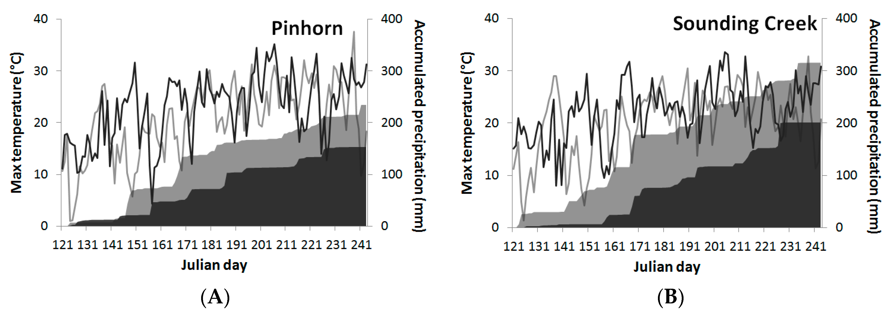
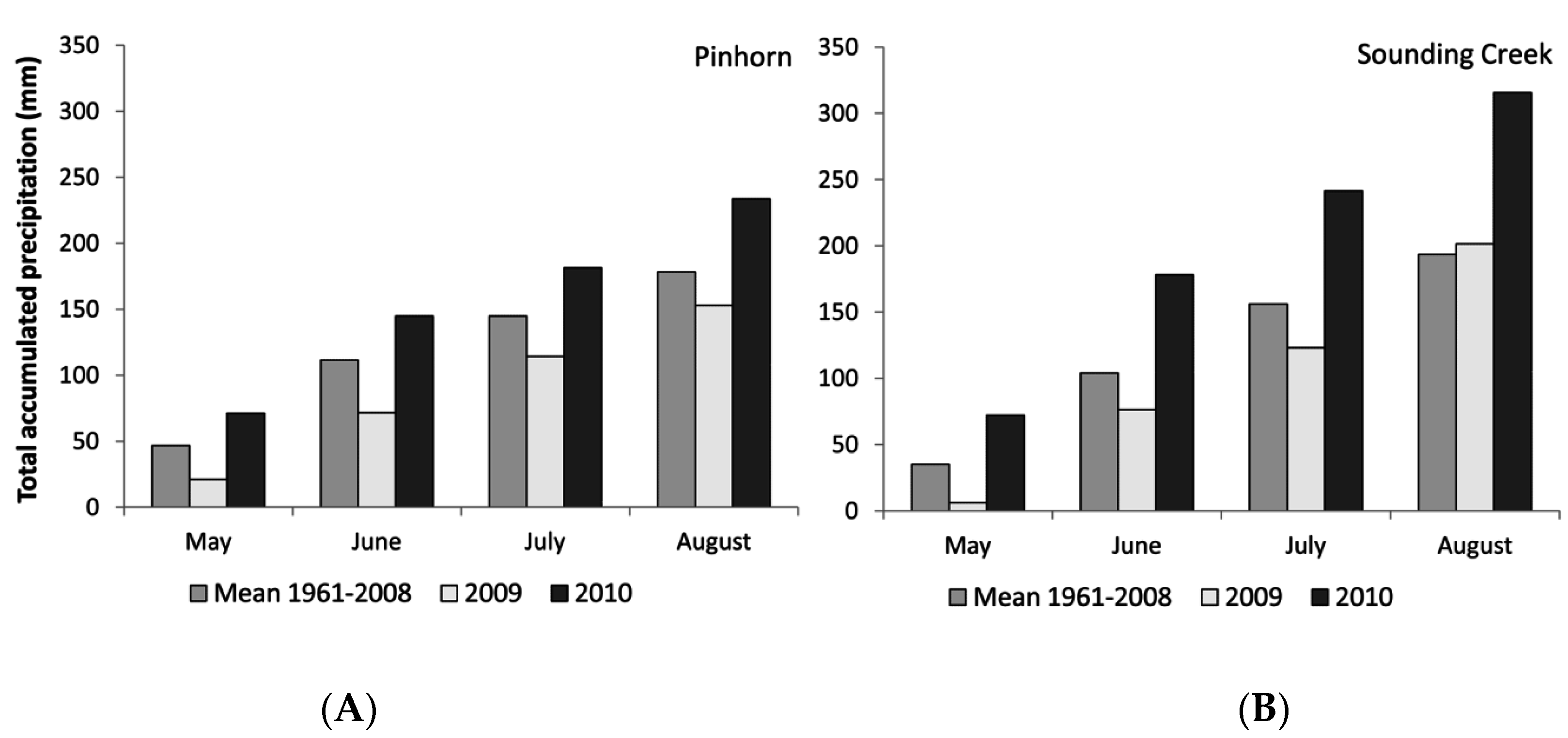
3.1. Precipitation and Temperature Patterns

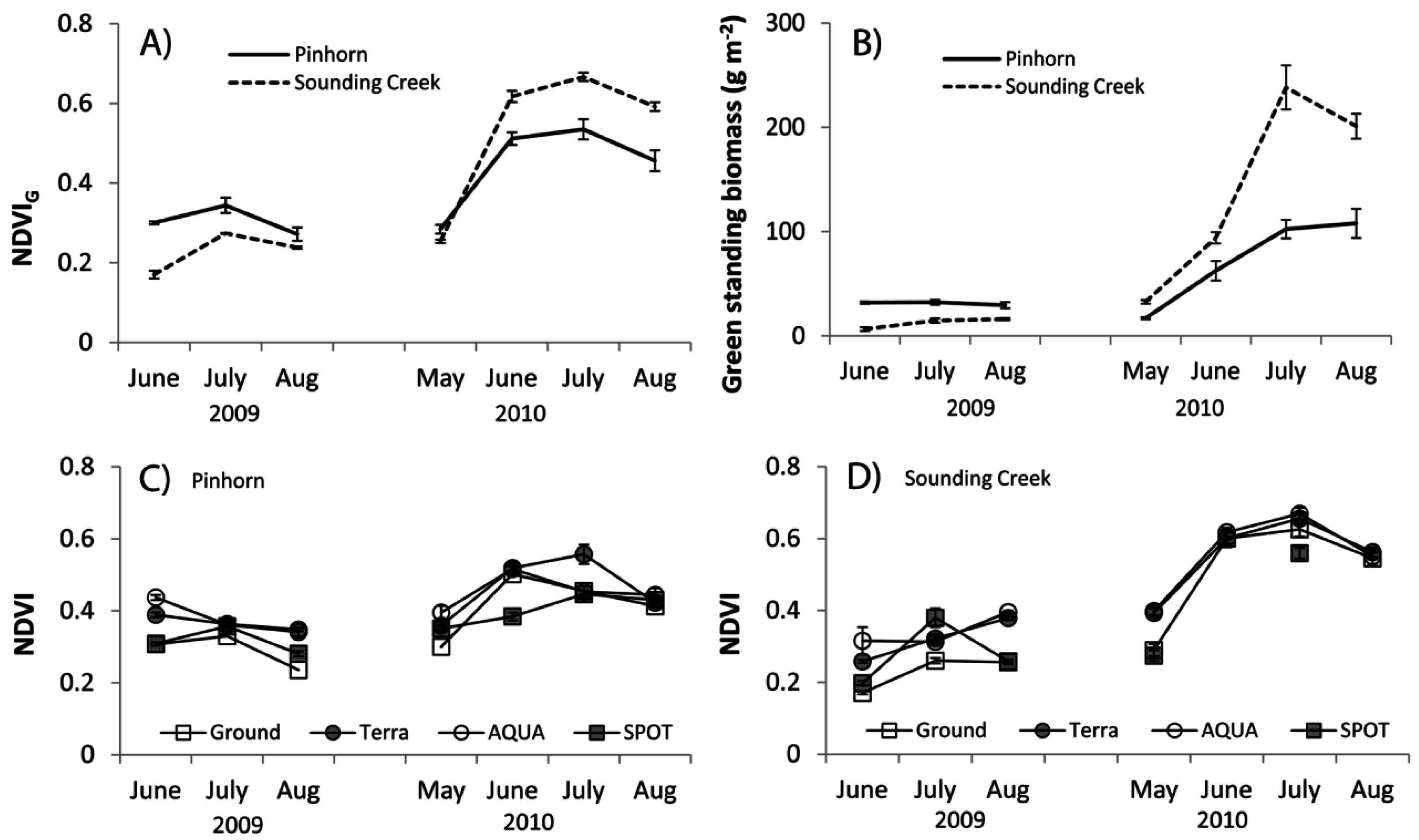
The summers of 2009 and 2010 provided extreme contrasts in weather conditions, with a significant difference in the amount of accumulated precipitation between the two summers (t-test; p < 0.001). The months of May and June were very dry in 2009, with comparatively high early growing season temperatures (Figure 3). The 2010 growing season experienced very wet conditions throughout the summer, with lower temperatures in the early months and much more temperature variability (Figure 3). The differences between the two growing seasons were more extreme in the Sounding Creek grazing reserve than in the Pinhorn. In 2009, the accumulated precipitation was lower than normal for both grazing reserves, with August in Sounding Creek being the only exception (Figure 4). In that year, accumulated precipitation in the early growing season was higher in the Pinhorn than in the Sounding Creek grazing reserve. In 2010 the accumulated precipitation was higher than normal for all months in both grazing reserves, although these differences were greater in Sounding Creek than in Pinhorn. These conditions produced a natural experiment characterized by drought in 2009 and above-normal rainfall in 2010 (relative to the 1961–2008 normal).

3.2. NDVI Patterns

In both grazing reserves, there was high year-to-year variation in NDVI (Figure 5). In 2009 and 2010 peak NDVI_G occurred in July for both locations (Figure 5A). Measurements of green standing biomass (largely graminoids) showed little seasonal variation in 2009 and greatly increased seasonal variation in 2010 (Figure 5B). The higher peak in Sounding Creek in 2010 reflected higher production and greater standing biomass in that year at that site. At Pinhorn, peak green biomass occurred in July in 2009, while in 2010 there was little difference in biomass between July and August (Figure 5B). The year-to-year trends in NDVI_G and green standing biomass both demonstrate greater productivity for both sites in 2010 relative to 2009 (Figure 5A,B). This pattern is also apparent in the satellite NDVI (Figure 5C,D). The MODIS NDVI values were generally higher than the NDVI from the ground spectrometer, particularly for low, early-season NDVI values. SPOT offered the least coverage and its seasonal NDVI patterns and values deviated from the MODIS satellites. In comparison to the MODIS platforms, the offset between the SPOT data and the ground NDVI was more variable (Figure 5).

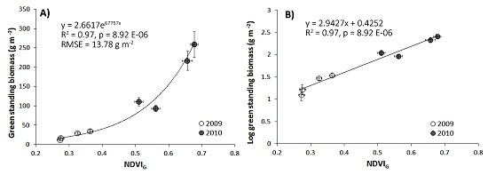
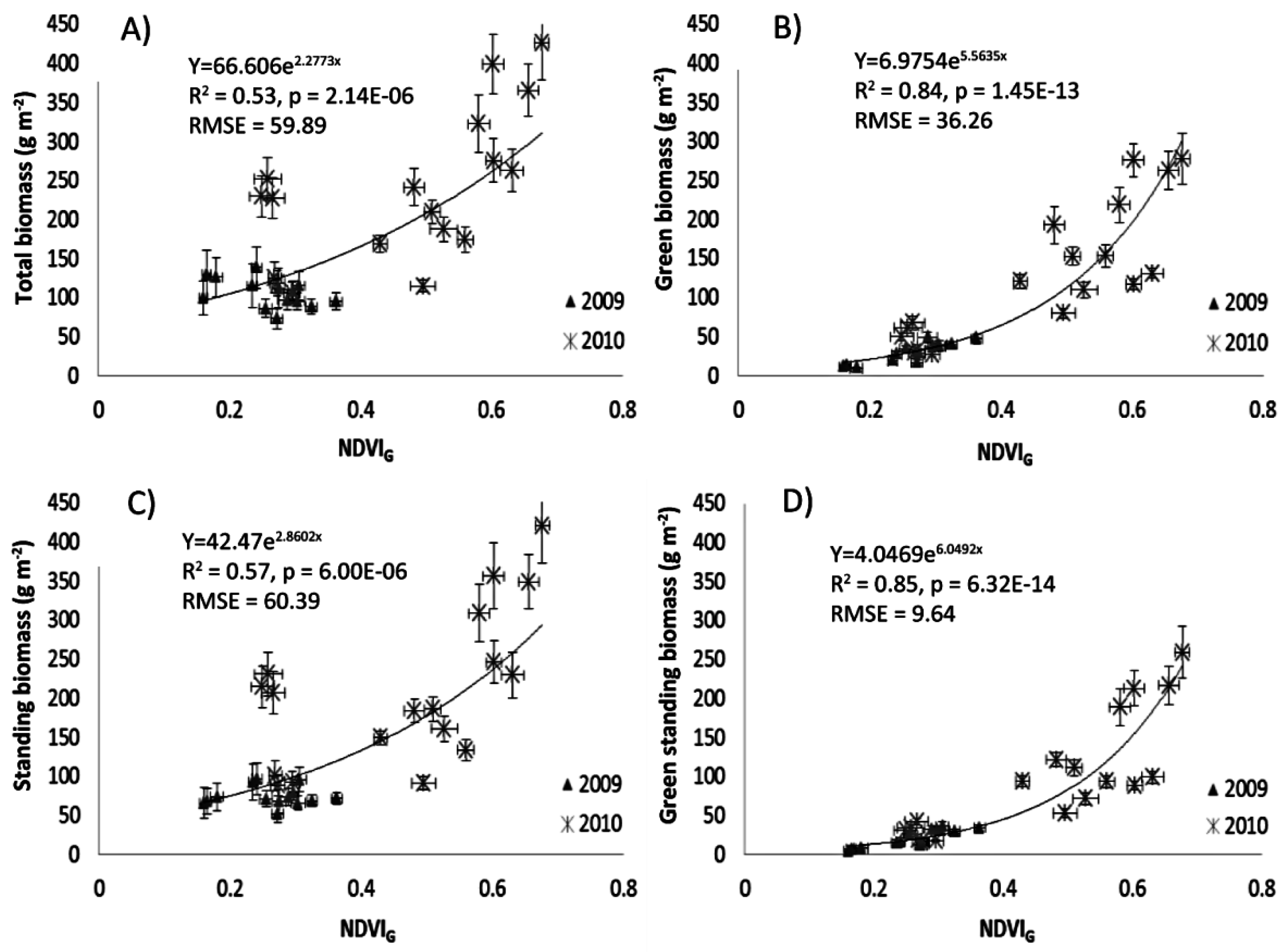
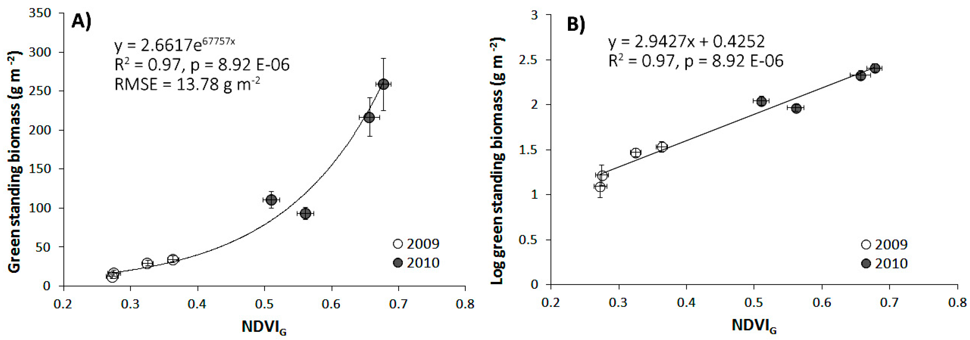
3.3. NDVI–Biomass Comparisons

Comparison of NDVI_G and the different metrics of biomass for all sampling dates and both sites yielded significant non-linear, exponential relationships (Figure 6). The correlations between NDVI_G and the green fraction of the biomass were much stronger than the total biomass and total standing biomass. Of all the biomass metrics, green standing biomass had the strongest correlation with NDVI_G (R² = 0.85).

The NDVI–biomass relationship was also examined for each month. The peak-season results yielded a stronger correlation (R² = 0.97, Figure 7) than the comparable figure using all-season data (R² = 0.85, Figure 6D). The cause of this improved correlation is evident in the seasonal progression in the NDVI-biomass relationship (see Figure S1, Supplementary Materials), and selection of peak-season (July) data greatly improved the overall NDVI–biomass fit (Figure 7). When the biomass data were log-transformed, the relationship between NDVI and green standing biomass became linear (cf. Figure 7A,B).

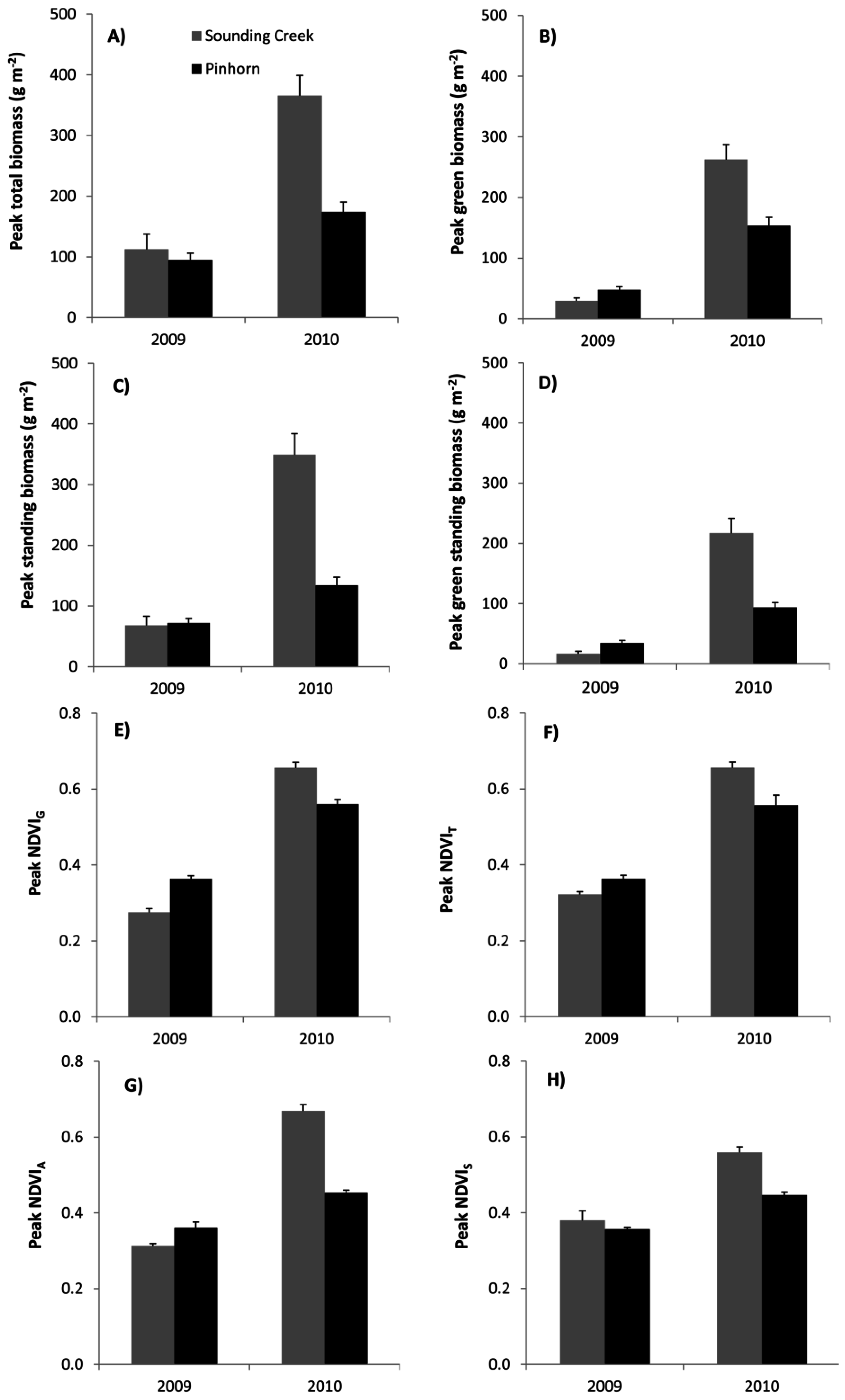
3.4. Interannual Comparisons

To highlight year-to-year differences in productivity, we summarized seasonal peak biomass and NDVI values by extracting the July values from the seasonal data. This choice to select peak values was made after observing a noticeable shift in the NDVI–biomass regressions during the growing season (see Figure S1, Supplementary Materials). Peak (July) biomass and NDVI values for both sites were much higher in 2010 (the wetter year) than in 2009 (the drier year) (Figure 8). In 2009, the Pinhorn grazing reserve had higher peak green biomass values than did the Sounding Creek grazing reserve, while in 2010 Sounding Creek was more productive, reflecting the contrasting precipitation patterns for these sites in these two years. In most cases, the July NDVI values showed the same patterns as peak green biomass. For both sites and years, the MODIS sensors (Aqua and Terra) produced NDVI patterns similar to green biomass and ground NDVI (NDVI_G). However, SPOT NDVI (NDVI_S) displayed slightly different interannual patterns; in 2009, NDVI_S exhibited a higher peak July NDVI for Sounding Creek (Figure 5D), which did not fit the patterns of the ground and MODIS NDVI values. In both growing seasons, NDVI_S indicated that Sounding Creek produced more new biomass than Pinhorn, which deviated from the observations from the MODIS and ground sensors.

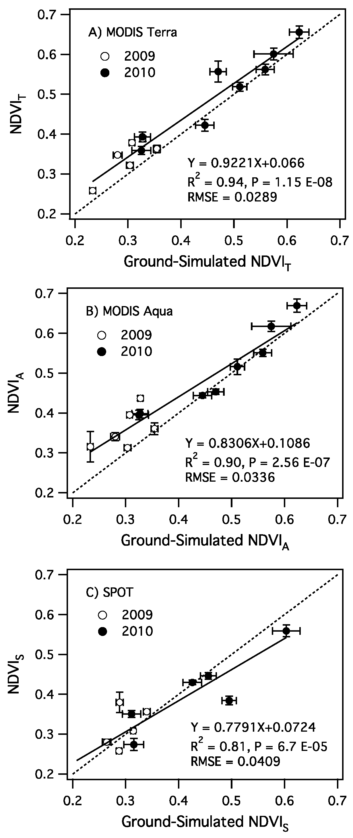
3.5. Sensor Comparisons

To further evaluate the MODIS and SPOT sensors for monitoring rangeland production, the NDVI from the different satellites for different months over both years were compared to the field-measured NDVI (NDVI_G) as a reference (Figure 9). For this comparison, the ground-measured NDVI collected from each 1-ha grid (Figure 2C) was recalculated to simulate each satellite sensor by convolving the spectral reflectance from field measurements against the satellite bands used for NDVI. When compared to these simulated NDVI values from ground measurements, NDVI from both MODIS platforms (NDVI_A and NDVI_T) provided similar offsets from the 1:1 line. The difference between NDVI from the Terra and Aqua platforms and the ground-simulated NDVI was greatest at the lower values, a pattern consistent with Figure 5 (where early-season MODIS values were notably higher than NDVI_G). Relative to the MODIS NDVI values, the SPOT NDVI (NDVI_S) values yielded a different offset pattern, showing higher values at low NDVI and lower values at high NDVI (Figure 9C). The slope of the regression between the ground-simulated NDVI and NDVI_S was significantly different than from the MODIS platforms, indicating clear differences between sensors (Terra vs. Aqua p = 0.645, Terra vs. SPOT p = 0.0004, Aqua vs. SPOT p = 0.0002). The strongest correlation between simulated NDVI and satellite-derived NDVI (and the lowest RMSE) was from the Terra platform (R² = 0.94, RMSE = 0.0289), followed by Aqua (R² = 0.9, RMSE = 0.0336; Figure 9). The SPOT satellite provided the weakest correlation (R² = 0.81) with simulated NDVI and the highest RMSE (RMSE = 0.0409, Figure 9).

4. Discussion

The weather conditions encountered during this study provided a natural experiment that provided a good test of the utility of remote sensing for monitoring interannual variation in yield. The precipitation differences in the two summers resulted in large differences in NDVI and biomass measurements between the two years for the two sites. Relative to single-year measurements, this interannual weather variability allowed a deeper understanding of the growth response of vegetation to varying moisture conditions, and allowed us to evaluate the ability of remote sensing to provide an accurate yield indicator across a wide range of growth responses typical of dry and wet years. Our findings of a large rainfall effect are consistent with the reports of Knapp and Smith (2001) and Camberlin et al. (2007), who observed that grasslands, such as the mixed prairie, have the capacity for large production response to uncommonly high precipitation [10,38]. Clearly, remote sensing methods provide an effective means for tracking year-to-year variation in above-ground green biomass as a result of different weather conditions in this prairie biome.

The time series of the NDVI calculated from the ground spectrometer, SPOT and the MODIS platforms all show trends that are similar to the standing biomass, indicating that there is a clear effect of seasonal and interannual weather patterns on NDVI and biomass, which can be monitored with different remote sensing methods. While the general NDVI trends were similar for the different sampling methods, the exact shapes were not the same, indicating some sensor differences. The two MODIS sensors yielded similar patterns, yet the data from Aqua demonstrate depressed NDVI values in July 2009 and 2010, in comparison to the Terra data. This is more clearly demonstrated by the correlations with ground NDVI (NDVI_G), where the offsets for the two platforms were very similar, yet the correlation was slightly stronger for Terra than Aqua. This slight difference between the two MODIS NDVI responses could be due to a variety of reasons, including specific calibration and instrument or sampling characteristics for each platform. Deering et al. (1992) found that at the FIFE prairie site sensor viewing angle and solar zenith angle had a large effect on vegetation indices [39]. Different viewing and solar zenith angles, in this case, would result from directly comparing data captured at different times of day, such that shadows and effects of surface anisotropy would affect the angular dependent signal due to the geometric configuration of the sun, sensor and target [40]. Independent field measurements [31] have shown a clear diurnal pattern for NDVI for prairie grassland, and this could have partly explained these differences between the two MODIS sensors having different overpass times.

Both MODIS sensors yielded NDVI values that were slightly higher than ground-measured NDVI, particularly at low NDVI values (Figure 5 and Figure 9). This offset did not appear to be a result of sensor band differences, because it was maintained in the comparison to simulated NDVI data that were designed to eliminate possible band configuration differences (Figure 9). The tendency of MODIS to produce values that are higher than the corresponding NDVI_G values calculated from ground spectrometers, has been previously reported for a chaparral site [41]. These authors speculated that this could be an effect of the data processing such as the atmospheric correction, which is applied to all MODIS data, or could be a specific characteristic of the sensor itself [41]; however, further studies need to be conducted to definitively explain this difference.

In comparison to the MODIS time series, the SPOT time series exhibited more scatter and a different offset when compared to ground-simulated NDVI (Figure 9). In July, the SPOT NDVI (NDVI_S) overestimated ground NDVI in 2009 and underestimated in 2010, particularly for Sounding Creek (Figure 5), which is made clearer by comparing the regression with the 1:1 line (Figure 9). This greater scatter in the SPOT NDVI than in the MODIS NDVI would make simple correction for the offset much more difficult and suggests SPOT would be less reliable than MODIS for monitoring variation in rangeland yield. In our study, the utility of the SPOT platform for monitoring year-to-year variability was limited by the inadequate time series capability resulting from restricted temporal coverage along with periodic cloud contamination. ATIC (the local SPOT data distributor) did not distribute SPOT images with greater than 10 percent cloud cover within the image; consequently, cloud-free SPOT imagery was unavailable for Sounding Creek in both June and August 2010 (Figure 5), making extensive, direct comparisons with MODIS and ground NDVI difficult. This reduced availability of SPOT data, combined with its high cost, precluded a fully equivalent sensor comparison.

Some studies [24] have suggested that SPOT is superior to MODIS for rangeland monitoring due to its higher spatial resolution. SPOT satellite imagery has a spatial resolution of 30 m, which resulted in decreased temporal resolution relative to MODIS, as the smaller field of view requires more orbits of the Earth to cover the same position [42]. In comparison to the daily coverage by the MODIS platforms, the 26-day temporal resolution of SPOT appeared to be inadequate to ensure repeat coverage of an area with data quality comparable to MODIS. While MODIS sensors have lower spatial resolution, the daily coverage allows creation of eight-day composites (employing maximum value compositing and bidirectional reflectance distribution function correction [37]), so errors due to clouds and other effects are reduced. The SPOT sensor can be directed off-nadir to increase the temporal coverage [24]; however, this introduces error due to altered sensor angle [42]. Based on the results of our study, we conclude that the MODIS sensor may actually be more effective than SPOT for mixed prairie yield monitoring and management, particularly when continuous time series are required over large areas.

A number of factors can introduce variability into the NDVI–biomass relationship. For example, scatter in the NDVI–green biomass relationship can be a result of different canopy architecture, which has an effect on NDVI [43], and this may lead to seasonal progression in the NDVI-biomass relationship (Figure S1). In May, the variation between NDVI and biomass is partly due to vegetation carryover from the previous year masking new growth. At the beginning of the growing season there had been little or no new green growth, with the initial growth likely to be hidden by the last season’s biomass (the carryover error). The greater variability in August is likely due to senescence, which causes a decline in chlorophyll content (which would affect NDVI); this gradually changing greenness was not fully considered by our harvesting method, which distinguished between green and brown vegetation but did not consider the varying degrees of green associated with changing pigment content at different growth and senescence stages. The effects of dead biomass on reducing the NDVI correlations with biomass are likely to be strongest at the beginning of the season (due to the “carryover” of dead standing biomass from the previous year) and towards the end of the season, when vegetation senescence has begun [44,45]. Our seasonal results could also have been influenced by the different species composition in the two townships, with Pinhorn having greater amounts of drought-resistant C₄ graminoids than the C₃ species dominant in Sounding Creek [46]. Together, these effects undoubtedly contributed to scatter in the NDVI–green biomass relationship when all seasons and sites are combined (R² = 0.85, Figure 6D). Focusing on the midsummer peak (July) values, as suggested by Butterfield and Malmstroem (2009) [45], effectively removed the early-season carryover error and the late-season senescence phase, and resulted in more accurate biomass estimation (R² = 0.97, Figure 8). Interestingly, despite the seasonal NDVI–green biomass shifts, there were strong correlations between peak-season (July) and end-of-season (August) values for NDVI_G (R² = 0.99, not shown) and log green standing biomass (R² = 0.99, not shown), suggesting a potential to estimate end-of-season biomass from peak-season measurements or vice versa.

Another potential source of error in NDVI measurements can be the background contamination from soil, litter, snow, surface wetness, or low-growing vegetation, which can confound satellite-based assessments of prairie productivity and ground cover [24,47]. For instance, Hall-Beyer and Gwyn (1996) determined that the presence of Selaginella densa, a mat-forming member of the fern phylum that is present in dry mixed-grass prairie, can also lead to errors in biomass estimates from optical remote sensing [48]. Selaginella densa mimics sparse grasses in NDVI measurements, yet it does not grow tall enough to be harvested with the methodology used here, so it was not included in our biomass data. Accounting for this effect could reduce scatter in the NDVI–green biomass relationship. By adapting the harvest sampling method to include very low-lying green vegetation in biomass estimates, this “background” green vegetation could be explicitly included in the analysis. Error resulting from this phenomenon would vary with rainfall and productivity. For example, drought could decrease the standing component of the vegetation and could allow more reflectance from lower canopy layers. On the other hand, early in the growing season during a drought year there can be more masking of the slowly emerging green biomass by the litter that is present from previous growing seasons (the carryover effect). This would decrease the amount of green vegetation visible to the spectrometer.

Both spatial aggregation and season affected the NDVI–biomass relationships (Figure S1), and these findings indicate that careful consideration of sample timing and methods of data aggregation is warranted when developing a biomass monitoring program from satellite data. Selection of peak-season data aggregated at the township scale (approximately 93 km²) largely removed these complications, and yielded a very strong agreement between NDVI and standing green biomass (Figure 9), allowing a clear comparison of year-to-year productivity differences (Figure 7). With the exception of SPOT NDVI, interannual changes in NDVI and standing green biomass (yield) were very similar for the different sensors (Figure 7), which indicates that NDVI can be an effective proxy for the standing green biomass in the dry mixed-grass prairie. The different shapes of these seasonal trends for NDVI and standing green biomass can be largely attributable to the non-linear relationship between NDVI and biomass (Figure 6 and Figure 8), which has been reported before [26,32].

The curvilinear relationship between green biomass and NDVI creates an apparent “saturation problem,” where over a certain value NDVI becomes almost invariant to changes in vegetation amount and/or condition [26,30,49]. This saturation, a natural result of the shape of the NDVI-biomass relationship [26], can largely be explained by the exponential extinction of radiation in vegetation canopies [50]. This relationship can be readily linearized by taking the log of biomass (Figure 8), revealing the true nature of the relationship between NDVI and biomass. From the perspective of determining absorbed radiation (f_APAR), a driving variable for production on this grassland ecosystem, there is less of a saturating problem; near-linear NDVI-f_APAR relationships are often obtained for grassland ecosystems, demonstrating that NDVI also provides an effective input for productivity models (e.g., the light-use efficiency model [31]). While our results indicate that NDVI saturation is not a serious constraint for biomass estimation in this mixed-grass prairie, this may not always be the case in more productive ecosystems.

The economic and ecological importance of the mixed prairie creates a need for accurate and cost-effective biomass monitoring. This study has demonstrated that remote sensing can accurately estimate biomass in these areas and that altered productivity due to interannual weather variability can be detected. These results are important for increasing the confidence of data users in the context of economic applications such as insurance payment programs and carbon markets. Ranchers’ perceptions of the accuracy of sampling methods are important for effective adoption and maintenance of remote sensing-based land management programs. Carbon markets would also require accurate monitoring in the mixed prairie, as varying climate and management regimes can undoubtedly influence sequestration. For such purposes, additional sampling (e.g., below-ground sampling) would also be needed. While further work would be required to demonstrate the full utility of NDVI for this purpose, this study strongly supports the use of satellite monitoring for estimating the above-ground component of productivity. Climate change is likely to result in more infrequent, intense precipitation in the areas being studied [1]. This study indicates that satellite methods can accurately monitor above-ground yield changes that are likely to occur with changing precipitation regimes due to interannual variability or as a result of changing climate.

5. Conclusions

Our results demonstrate accurate NDVI-based estimates of biomass production and phenology in a mixed-grass prairie, although seasonal shifts in the NDVI–biomass relationships emerged from temporal patterns of carryover and senescence. These findings indicate that careful consideration of sample timing to consider seasonal effects on the NDVI–biomass relationship is warranted when developing a biomass monitoring program from satellite data. Midsummer peak values avoid the early-season carryover error and the late-season senescence phase, providing the most accurate biomass estimation (R² = 0.97). Similarly, averaging field data to the township level greatly improved the agreement with satellite data, illustrating the importance of spatial aggregation when comparing data from vastly different scales. This approach demonstrates the value of applying experimental methods to remotely sensed data collected in different ways, and at different times and spatial scales. With these methods, the changes in biomass due to variable precipitation between the two years was clearly identifiable; NDVI illustrated that the wetter 2010 growing season had much greater biomass than the drier 2009 season. Clearly, the inter-annual vegetation and NDVI patterns were affected by the moisture regime available for plant growth during the two growing seasons studied. The MODIS Terra platform provided the best estimate of NDVI of the three satellite platforms studied, followed closely by the MODIS Aqua platform, and SPOT provided the least accurate estimates, in part due to the more limited SPOT coverage. We conclude that satellite NDVI, calibrated against field measurements, is a powerful tool for monitoring yield in a dry mixed-grass prairie ecosystem and can benefit ongoing management efforts. Future studies could focus on combining yield monitoring with other co-benefits, including habitat, biodiversity, and carbon sequestration.

References

1. Fay, P.A.; Carlisle, J.D.; Knapp, A.K.; Blair, J.M.; Collins, S.L. Productivity responses to altered rainfall patterns in a C4-dominated grassland. Oecologia 2003, 137, 245–251. [Google Scholar] [CrossRef] [PubMed]
2. Schino, G.; Borfecchia, F.; De Cecco, L.; Dibari, C.; Iannetta, M.; Martini, S.; Pedrotti, F. Satellite estimate of grass biomass in a mountainous range in central Italy. Agrofor. Syst. 2003, 59, 157–162. [Google Scholar] [CrossRef]
3. Kustas, W.P.; Goodrich, D.C.; Moran, M.S.; Amer, S.A.; Bach, L.B.; Blanford, J.H.; Chehbouni, A.; Claassen, H.; Clements, W.E.; Doraiswamy, P.C.; et al. An interdisciplinary field study of the energy and water fluxes in the atmosphere-biosphere system over semiarid rangelands: Description and some preliminary results. Bull. Am. Meteorol. 1991, 72, 1683–1705. [Google Scholar] [CrossRef]
4. Sims, P.L.; Risser, P.G. Grasslands. In North American Terrestrial Vegetation; Barbour, M.G., Billings, W.D., Eds.; Cambridge University Press: Cambridge, UK, 2000; pp. 324–356. [Google Scholar]
5. Coupland, R.T. A reconsideration of grassland classification in the northern great plains of North America. J. Ecol. 1961, 49, 135–167. [Google Scholar] [CrossRef]
6. Adams, B.W.; Poulin-Klein, L.; Moisey, D.; McNeil, R.L. Rangeland Plant Communities and Range Health Assessment Guidelines for The Dry Mixedgrass Natural Subregion of Alberta; Rangeland Management Branch, Public Lands Division, Alberta Sustainable Resource Development: Lethbridge, AB, Canada, 2005. [Google Scholar]
7. Paruelo, J.M.; Lauenroth, W.K. Interannual variability of NDVI and its relationship to climate for North American shrublands and grasslands. J. Biogeogr. 1998, 25, 721–733. [Google Scholar] [CrossRef]
8. Bedard, F.; Crump, S.; Gaudreau, J. A comparison between terra MODIS and NOAA AVHRR NDVI satellite image composites for the monitoring of natural grassland conditions in Alberta, Canada. Can. J. Remote Sens. 2006, 32, 44–50. [Google Scholar] [CrossRef]
9. Churkina, G.; Running, S.W. Contrasting climatic controls on the estimated productivity of global terrestrial biomes. Ecosystems 1998, 1, 206–215. [Google Scholar] [CrossRef]
10. Knapp, A.K.; Smith, M.D. Variation among biomes in temporal dynamics of aboveground primary production. Science 2001, 291, 481–484. [Google Scholar] [CrossRef] [PubMed]
11. Groisman, P.Y.; Karl, T.R.; Easterling, D.R.; Knight, R.W.; Jamason, P.F.; Hennessy, K.J.; Suppiah, R.; Page, C.M.; Wibig, J.; Fortuniak, K.; et al. Changes in the probability of heavy precipitation: Important indicators of climatic change. Clim. Chang. 1999, 42, 243–283. [Google Scholar] [CrossRef]
12. Bernhardt-Roemermann, M.; Roemermann, C.; Sperlich, S.; Schmidt, W. Explaining grassland biomass—The contribution of climate, species and functional diversity depends on fertilization and mowing frequency. J. Appl. Ecol. 2011, 48, 1088–1097. [Google Scholar] [CrossRef]
13. Rowley, R.J.; Price, K.P.; Kastens, J.H. Remote sensing and the rancher: Linking rancher perception and remote sensing. Rangel. Ecol. Manag. 2007, 60, 359–368. [Google Scholar] [CrossRef]
14. Hunt, E.R.; Everitt, J.H.; Ritchie, J.C.; Moran, M.S.; Booth, D.T.; Anderson, G.L.; Clark, P.E.; Seyfried, M.S. Applications and research using remote sensing for rangeland management. Photogramm. Eng. Remote Sens. 2003, 69, 675–693. [Google Scholar] [CrossRef]
15. Svejcar, T.; Angell, R.; Bradford, J.A.; Dugas, W.; Emmerich, W.; Frank, A.B.; Gilmanov, T.; Haferkamp, M.; Johnson, D.A.; Mayeux, H.; et al. Carbon fluxes on North American rangelands. Rangel. Ecol. Manag. 2008, 61, 465–474. [Google Scholar] [CrossRef]
16. Wang, R.; Gamon, J.A.; Emmerton, C.A.; Li, H.; Nestola, E.; Pastorello, G.Z.; Menzer, O. Integrated analysis of productivity and biodiversity in a southern Alberta prairie. Remote Sens. 2016, 8, 214. [Google Scholar] [CrossRef]
17. Wang, R.; Gamon, J.A.; Montgomery, R.A.; Townsend, P.A.; Zygielbaum, A.I.; Bitan, K.; Tilman, D.; Cavender-Bares, J. Seasonal variation in the NDVI-species richness relationship in a prairie grassland experiment (Cedar Creek). Remote Sens. 2016. [Google Scholar] [CrossRef]
18. Booth, D.T.; Tueller, P.T. Rangeland monitoring using remote sensing. Arid Land Res. Manag. 2003, 17, 455–467. [Google Scholar] [CrossRef]
19. Tucker, C.J.; Miller, L.D.; Pearson, R.L. Shortgrass prairie spectral measurements. Photogramm. Eng. Remote Sens. 1975, 41, 1157–1162. [Google Scholar]
20. Bork, E.W.; West, N.E.; Price, K.P.; Walker, J.W. Rangeland cover component quantification using broad (TM) and narrow-band (1.4 nm) spectrometry. J. Range Manag. 1999, 52, 249–257. [Google Scholar] [CrossRef]
21. Pineiro, G.; Oesterheld, M.; Paruelo, J.M. Seasonal variation in aboveground production and radiation-use efficiency of temperate rangelands estimated through remote sensing. Ecosystems 2006, 9, 357–373. [Google Scholar] [CrossRef]
22. Reeves, M.C.; Winslow, J.C.; Running, S.W. Mapping weekly rangeland vegetation productivity using MODIS algorithms. J. Range Manag. 2001, 54, A90–A105. [Google Scholar]
23. SPOT Satellite Imagery. EARTH Observation, Satellite and Geo-Information. Available online: http://www.webcitation.org/6h5b1pN83 (accessed on 18 January 2012).
24. Grant, K.M.; Johnson, D.L.; Hildebrand, D.V.; Peddle, D.R. Quantifying biomass production on rangeland in southern Alberta using SPOT imagery. Can. J. Remote Sens. 2012, 38, 695–708. [Google Scholar] [CrossRef]
25. Tucker, C.J.; Vanpraet, C.L.; Sharman, M.J.; Vanittersum, G. Satellite remote-sensing of total herbaceous biomass production in the Senegalese Sahel—1980–1984. Remote Sens. Environ. 1985, 17, 233–249. [Google Scholar] [CrossRef]
26. Gamon, J.A.; Field, C.B.; Goulden, M.L.; Griffin, K.L.; Hartley, A.E.; Joel, G.; Penuelas, J.; Valentini, R. Relationships between NDVI, canopy structure, and photosynthesis in three Californian vegetation types. Ecol. Appl. 1995, 5, 28–41. [Google Scholar] [CrossRef]
27. Huete, A.R.; Tucker, C.J. Investigation of soil influences in AVHRR red and near-infrared vegetation index imagery. Int. J. Remote Sens. 1991, 12, 1223–1242. [Google Scholar] [CrossRef]
28. Washington-Allen, R.A.; West, N.E.; Ramsey, R.D.; Efroymson, R.A. A protocol for retrospective remote sensing-based ecological monitoring of rangelands. Rangel. Ecol. Manag. 2006, 59, 19–29. [Google Scholar] [CrossRef]
29. Guo, X.; Price, K.P.; Stiles, J.M. Modeling biophysical factors for grasslands in eastern Kansas using Landsat TM data. Trans. Kans. Acad. Sci. 2000, 103, 122–138. [Google Scholar] [CrossRef]
30. Frank, A.B.; Karn, J.F. Vegetation indices, CO2 flux, and biomass for northern plains grasslands. J. Range Manag. 2003, 56, 382–387. [Google Scholar] [CrossRef]
31. Nestola, E.; Calfapietra, C.; Emmerton, C.A.; Wong, C.Y.; Thayer, D.R.; Gamon, J.A. Monitoring grassland seasonal carbon dynamics, by integrating MODIS NDVI, proximal optical sampling, and eddy covariance measurements. Remote Sens. 2016. [Google Scholar] [CrossRef]
32. Gamon, J.A.; Field, C.B.; Roberts, D.A.; Ustin, S.L.; Valentini, R. Functional patterns in an annual grassland during an AVIRIS overflight. Remote Sens. Environ. 1993, 44, 239–253. [Google Scholar] [CrossRef]
33. Gamon, J.A.; Cheng, Y.F.; Claudio, H.; MacKinney, L.; Sims, D.A. A mobile tram system for systematic sampling of ecosystem optical properties. Remote Sens. Environ. 2006, 103, 246–254. [Google Scholar] [CrossRef]
34. Rao, K.N. Index based crop insurance. In Proceedings of the International Conference on Agricultural Risk and Food Security 2010, Beijing, China, 10–12 June 2010.
35. Morisette, J.T.; Privette, J.L.; Justice, C.O. A framework for the validation of MODIS land products. Remote Sens. Environ. 2002, 83, 77–96. [Google Scholar] [CrossRef]
36. Cohen, W.B.; Justice, C.O. Validating MODIS terrestrial ecology products: Linking in situ and satellite measurements. Remote Sens. Environ. 1999, 70, 1–3. [Google Scholar] [CrossRef]
37. NASA (National Aeronautics and Space Administration). MODISWeb. Available online: http://MODIS.gsfc.nasa.gov/about/ (accessed on 18 January 2012).
38. Camberlin, P.; Martiny, N.; Philippon, N.; Richard, Y. Determinants of the interannual relationships between remote sensed photosynthetic activity and rainfall in tropical Africa. Remote Sens. Environ. 2007, 106, 199–216. [Google Scholar] [CrossRef]
39. Deering, D.W.; Middleton, E.M.; Irons, J.R.; Blad, B.L.; Waltershea, E.A.; Hays, C.J.; Walthall, C.; Eck, T.F.; Ahmad, S.P.; Banerjee, B.P. Prairie grassland bidirectional reflectances measured by different instruments at the FIFE site. J. Geophys. Res. Atmos. 1992, 97, 18887–18903. [Google Scholar] [CrossRef]
40. Huete, A.; Justice, C.; Liu, H. Development of vegetation and soil indices for MODIS-EOS. Remote Sens. Environ. 1994, 49, 224–234. [Google Scholar] [CrossRef]
41. Cheng, Y.F.; Gamon, J.A.; Fuentes, D.A.; Mao, Z.Y.; Sims, D.A.; Qiu, H.L.; Claudio, H.; Huete, A.; Rahman, A.F. A multi-scale analysis of dynamic optical signals in a southern California chaparral ecosystem: A comparison of field, AVIRIS and MODIS data. Remote Sens. Environ. 2006, 103, 369–378. [Google Scholar] [CrossRef]
42. Tueller, P.T. Remote-sensing technology for rangeland management applications. J. Range Manag. 1989, 42, 442–453. [Google Scholar] [CrossRef]
43. Sellers, P.J. Canopy reflectance, photosynthesis and transpiration. Int. J. Remote Sens. 1985, 6, 1335–1372. [Google Scholar] [CrossRef]
44. Cyr, L.; Bonn, F.; Pesant, A. Vegetation indices derived from remote sensing for an estimation of soil protection against water erosion. Ecol. Model. 1995, 79, 277–285. [Google Scholar] [CrossRef]
45. Butterfield, H.S.; Malmstrom, C.M. The effects of phenology on indirect measures of aboveground biomass in annual grasses. Int. J. Remote Sens. 2009, 30, 3133–3146. [Google Scholar] [CrossRef]
46. Davidson, A.; Csillag, F. A comparison of three approaches for predicting C4 species cover of northern mixed grass prairie. Remote Sens. Environ. 2003, 86, 70–82. [Google Scholar] [CrossRef]
47. Smith, A.M.; Hill, M.J.; Zhang, Y.Q. Estimating ground cover in the mixed prairie grassland of southern Alberta using vegetation indices related to physiological function. Can. J. Remote Sens. 2015, 41, 51–66. [Google Scholar] [CrossRef]
48. Hall-Beyer, M.; Gwyn, Q.H.J. Selaginella densa reflectance: Relevance to rangeland remote sensing. J. Range Manag. 1996, 49, 470–473. [Google Scholar] [CrossRef]
49. Walthall, C.L.; Middleton, E.M. Assessing spatial and seasonal-variations in grasslands with spectral reflectances from a helicopter platform. J. Geophys. Res. Atmos. 1992, 97, 18905–18912. [Google Scholar] [CrossRef]
50. Sellers, P.J. Canopy reflectance, photosynthesis, and transpiration 2: The role of biophysics in the linearity of their interdependence. Remote Sens. Environ. 1987, 21, 143–183. [Google Scholar] [CrossRef]
Figure 1. Location of study, showing the Sounding Creek and Pinhorn grazing reserves in Southern Alberta, Canada (A); Each grazing reserve contained 10 sampling locations (yellow circles, (B,C)).
Remotesensing 08 00872 g001
Figure 2. Sample SPOT image (A), showing field sampling sites (yellow dots) for the Pinhorn grazing reserve in 2009. (B) A detailed image of these sites, along with the single MODIS pixel (parallelogram) best corresponding to the centermost field sampling site. Each sampling site contained several 1-m diameter optical sampling plots (circles) (C) coincident with biomass harvestings sites (rectangles) (C) that were used for NDVI calibration against biomass. Each sampling site also included a 1-hectare (100 m × 100 m) sampling grid (C) that was used for comparison of ground NDVI to satellite NDVI measurements. See Section 2.2, Section 2.3 and Section 2.4 for field sampling protocols.
Remotesensing 08 00872 g002
Figure 3. Maximum air temperature (lines) and accumulated precipitation (shadow) versus Julian day for the months of May, June, July and August in 2009 (black lines and shading) and 2010 (grey lines and shading) for the Pinhorn grazing reserve (A) and the Sounding Creek grazing reserve (B). The meteorological data are courtesy of Alberta Agriculture and Forestry.
Remotesensing 08 00872 g003
Figure 4. Comparison of the normal accumulated precipitation (mean calculated over 1961 to 2008) to the accumulated precipitation measured at the Pinhorn grazing reserve (A) and the Sounding Creek grazing reserve (B) in the 2009 and 2010 growing seasons. The meteorological data are courtesy of Alberta Agriculture and Forestry.
Remotesensing 08 00872 g004
Figure 5. Time series of NDVI derived from ground spectrometry (NDVIG) (A) and harvested green fraction of the standing biomass (B) from both grazing reserves as well as the time series of NDVI from ground spectrometer data, MODIS data from the Terra and Aqua platforms, and SPOT data from the Pinhorn grazing reserve (C) and Sounding Creek grazing reserve (D) during the summers of 2009 and 2010. Note that SPOT coverage was missing in June and August 2010 for Sounding Creek. For comparison, average NDVI values for bare soil were approximately 0.1 at these sites. Error bars denote the standard error of the mean.
Remotesensing 08 00872 g005
Figure 6. Relationship between NDVI and biomass for the Sounding Creek and Pinhorn grazing reserves in the 2009 and 2010 combined growing seasons. Regressions between NDVIG (X variable) and several expressions of biomass (Y variables), including Total Biomass (A); Green Biomass (B); Standing Biomass (C); and Standing Green Biomass (D). Exponential fits and regression statistics (R2, p, and RMSE values) are also shown. Error bars are the standard error of the mean. See Table 1 for further explanation of biomass metrics.
Remotesensing 08 00872 g006
Figure 7. Relationships between peak (July) NDVIG and peak (July) green standing biomass for the combined Sounding Creek and Pinhorn grazing reserves in 2009 and 2010 (A); Also shown is the effect of log transformation on the form of the relationship (B). Data have been aggregated to the township level by averaging 10 sites per township. Error bars denote standard error of the mean.
Remotesensing 08 00872 g007
Figure 8. July (peak) values for total biomass (A); green biomass (B); standing biomass (C); green standing biomass (D); NDVI from ground spectrometry (E); and NDVI derived from the Terra (F); Aqua (G) and SPOT (H) satellites from the Sounding Creek and Pinhorn grazing reserves in the 2009 and 2010 growing seasons. Error bars denote the standard error of the mean.
Remotesensing 08 00872 g008
Figure 9. Ground-simulated NDVI vs. satellite NDVI for MODIS Terra (A); MODIS Aqua (B); and SPOT (C). Data from 2009 and 2010 are distinguished by different symbols, as indicated on each panel. Ground-simulated NDVI was derived using MODIS or SPOT band passes, as described in Section 2. Also shown are the 1:1 lines (dotted lines) and the best-fit regression lines (solid lines) for each comparison, along with regression equations, relevant statistics, and RMSE values. Error bars indicate the standard error of the mean.
Remotesensing 08 00872 g009