The Effects of Spatiotemporal Changes in Land Degradation on Ecosystem Services Values in Sanjiang Plain, China

Abstract

Sanjiang Plain has undergone dramatic land degradation since the 1950s, which has caused negative effects on ecosystems services and sustainability. In this study, we used trajectory analysis as well as the Lorenz curve, Gini coefficient and relative land use suitability index (R) to analyze spatiotemporal changes of land degradation from 1954 to 2013 and to make a preliminary estimation of the role of human activities in observed environmental changes using a five-stage LULC data. This study also explored the effect of land degradation on the values and structure of ecosystem services. Our results indicated that more than 70% of marsh area originally present in the study area has been lost, whereas less than 30% was preserved. Dry farmland and paddy increased rapidly at the expense of marsh, forest and grassland. Land use structure became more unsuitable during the past 60 years. Compared with natural factors, human activities played a dominant role (89.67%) in these changes. This dramatic land degradation caused the significant loss of ecosystem services values and the changes in the structure of ecosystem services. These results confirmed the effectiveness of combining temporal trajectory analysis, the Lorenz curve/Gini coefficient and the R index in analyzing spatiotemporal changes in progressive land degradation. Also, these findings highlight the necessity of separating dry farmland from paddy when studying land degradation changes and the effects on ecosystem services in regions where dry farmland has often been converted to paddy.

1. Introduction

As one of the most important indicators in understanding the interactions between human activities and the environment [1,2], land use and land cover change (LULCC) plays a pivotal role in global ecological and environmental changes [3,4,5,6,7]. LULCC analysis is an important tool for assessing global change at various spatial and temporal scales [3]. LULCC could have significant impacts on a number of interrelated biogeochemical processes and eventually lead to global change [8]. Human activities play a pivotal role in LULCC [9]. Both anthropogenic factors and natural factors play an important role in LULCC; however, anthropogenic LULCC is now unprecedentedly large, profoundly affecting the Earth’s ecological systems [1,9]. Human-induced LULCC affects key aspects of earth system functioning and it has a significant negative impact on ecosystems [5]. For instance, it influences the global carbon cycle, and contributes to the increase in atmospheric CO₂ [10]. It is therefore important to study LULCC, so that its effects on terrestrial ecosystems can be discerned and sustainable land use planning can be carried out [11]. Additionally, quantification of the role of humans in LULCC is important for predicting land use changes as well as promoting the sustainable use of land resources [12,13,14], especially in ecologically fragile regions. However, research that quantifies of the role of humans in LULCC is still rare.

Previous studies typically used the bitemporal detection method to analyze spatiotemporal changes between pairs of time periods [5,6,7,8]. Trajectory analysis can recover the history of land cover change and can also relate the spatiotemporal pattern of such changes to other environmental and human factors [15,16]. It can also effectively analyze the trends of land use and land cover change over time [17,18]. Attempts have been made to apply a trajectory analysis method for assessing LULCC over multiple points in time [15,16,17,18,19,20,21]. To better understand land degradation progress and study the impact of human activities on the changes in natural environment, trajectory analysis was used in this study.

Land use structure could reflect the geographic configuration and comparison of different land use types [22]. Analyzing land use structure could help us better understand the relationship between land use and ecosystems, as well as the regional differences in the proportions of certain land use types [22,23]. Many methods have been used in studying land use structure, such as the artificial neural networks (ANN) [24,25], information entropy [26], optimal linear programming methods [27], and the Lorenz curve and the associated Gini coefficient [28,29]. The Lorenz curve originated from economics models and has been applied in many fields. 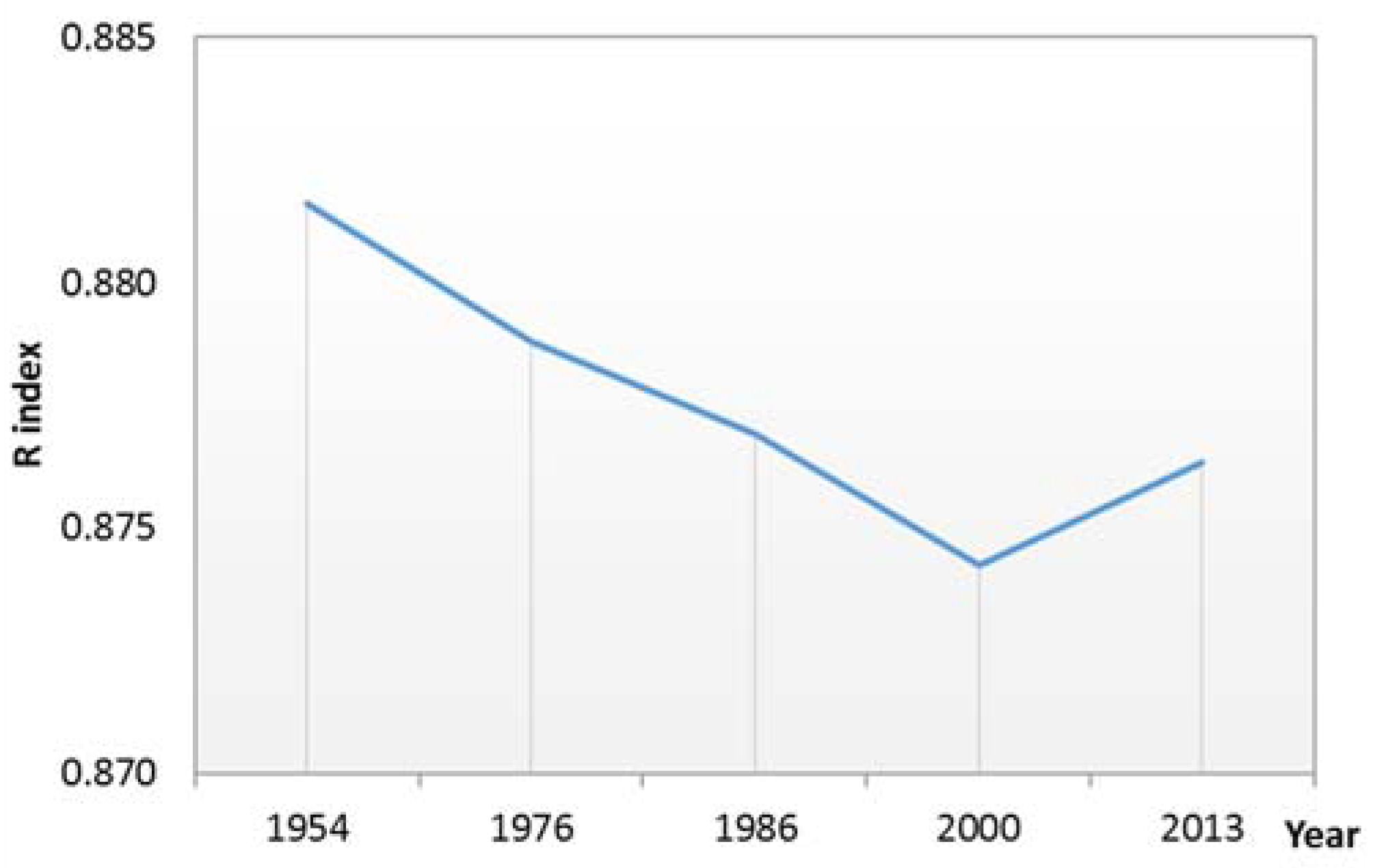The Lorenz curve and Gini coefficient can reveal and quantify the changes in land use structure and are simpler than other methods [22,29]. 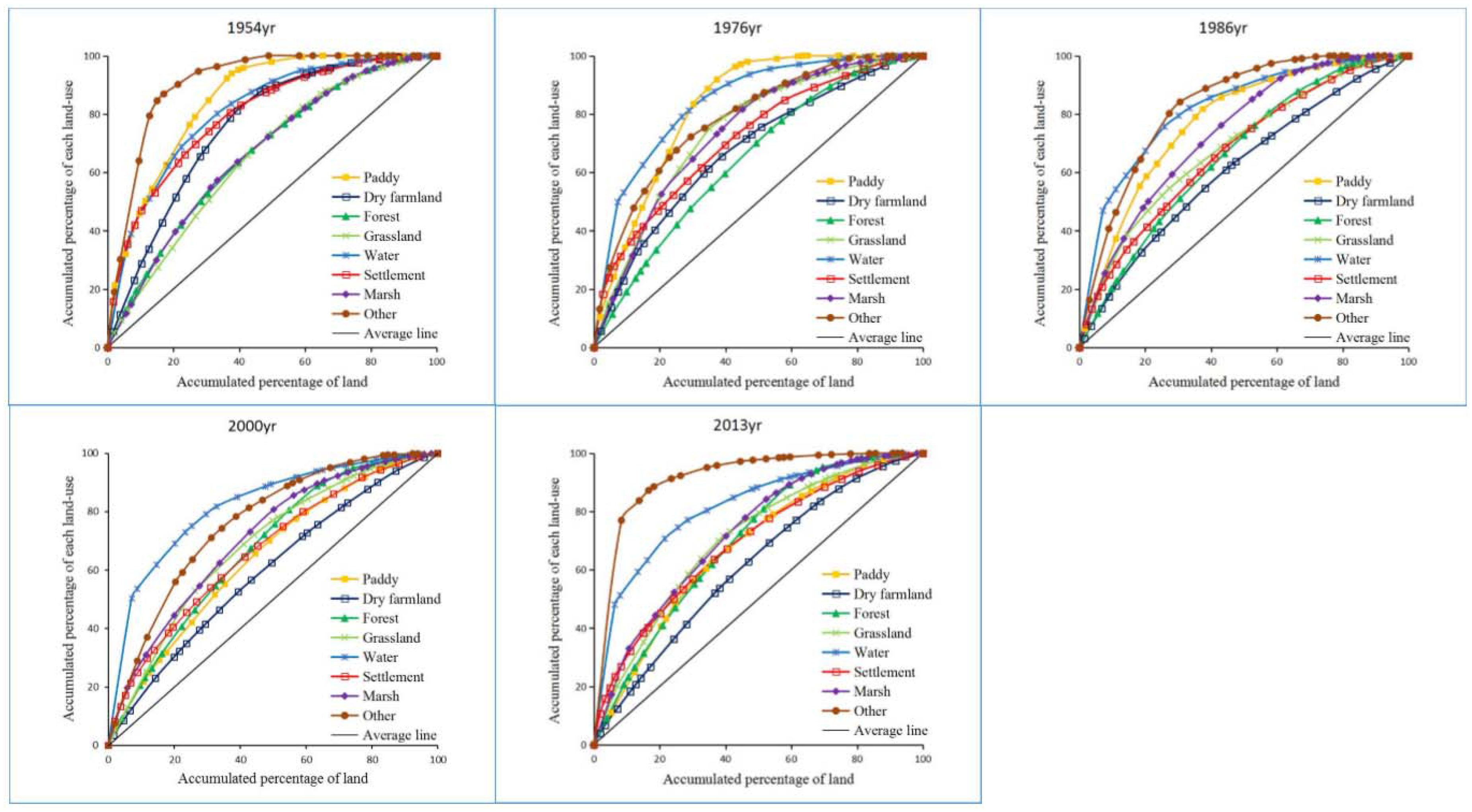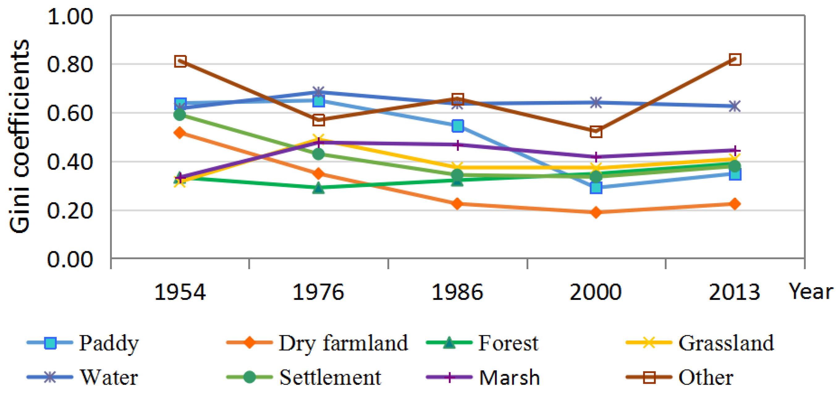The relative land-use suitability index (R) [16,30] can be used to assess the suitability of land-use structure. Larger R-values mean that the land use structure is more suitable than lower values. In this study, the Lorenz curve, Gini coefficient and R index were combined to analyze the land use structure of Sanjiang Plain.

Ecosystem services represent the benefits that living organism derived from ecosystem functions, which are necessary for human well-being, health, livelihoods, and survival [31,32,33,34]. Ecosystems supply goods that are necessary for human survival; maintain the earth’s life support systems; and provide entertainment for human beings [35,36]. Since the United Nations published its Millennium Ecosystem Assessment, many ecologists and economists have paid greater attention to the concept of ecosystem services [37,38] and interest in ecosystem services values (ESV) has grown quickly [38,39]. Various methods have been developed to estimate ESV [23,40,41,42,43,44]. By summarizing literature, Costanza et al. [31] grouped the ecosystem services into 10 biomes and classified the ecosystem services into 17 types to calculate global ESV. This method provides a reference for assessing ESV comprehensively [45] and has been applied successfully to specific areas, species, and ecosystems [37,46]. By surveying more than 200 ecologists from China, Xie et al. [43,47,48] modified the evaluation model proposed by Costanza to meet China’s specific situation. The table of ESV per unit area of different ecosystems proposed by Xie et al. is comprehensive and specific to China [34,45]. As a type of human-made wetland, the ESV of paddy field are quite different from those of dry farmland. However, there are still no standard estimates of ESV per unit area for paddy or dry farmland. Considering this situation and the specific condition of Sanjiang Plain, we modified Xie’s table based on net primary productivity (NPP) [34,49].

Dramatic land degradation often affects ecosystems services negatively [50]. Few studies have evaluated the impact of LULCC on ESV with the goal of providing useful insights into landscape planning and sustainable use of land resources [51,52]. Integrating LULCC and ESV into landscape planning for sustainable development is still a challenge [51,53,54,55]. As the largest freshwater marsh in China, Sanjiang Plain is vulnerable to global change and human disturbance. High-intensity human activities, especially large-scale reclamation, have led to intensive land degradation since the 1950s in this region [56,57,58,59]. Meanwhile, climate change [60], elevated atmospheric CO₂ [61], and other natural factors [59] have also caused some degree of land degradation in this region. Many studies [56,57,58,62,63] have examined spatiotemporal changes in land degradation and its driving factors over part or all of Sanjiang Plain. However, information on the land use structure changes and quantitative analysis of human impacts are still lacking for this area. Song et al. [56] found that paddy and dry farmland had different change processes by analyzing social statistics data and Liu et al. [64] found that paddy and dry farmland were frequently changed to other LULC types in northeast China. However, important characteristics of LULCC between paddy, dry farmland and other LULC types remain uncertain, especially the spatial pattern of these changes. Also, separating dry farmland from paddy is needed to estimate the values and structure of ecosystem services in this region. The objectives of this study include: (1) to analyze the spatiotemporal changes and changes in spatial structure of land degradation in the study area; (2) to estimate the role of human activities on land degradation in Sanjiang Plain quantitatively; and (3) to discuss the effects of land degradation on ESV change in the study area in order to provide scientific information to inform sustainable use of land resources.

2. Materials and Methods

2.1. Study Area

This work was conducted in the Sanjiang Plain (Figure 1) (45°01′05″N–48°27′56″N，130°13′10″E–135°05′26″E), northeast of China. The Sanjiang Plain is built up of sediment deposited by the Amur, Ussuri and Songhua Rivers. It includes the largest freshwater marshy wetland in China. Sanjiang Plain has 23 counties and covers an area of 108,900 km². The average annual precipitation ranges from 500 to 650 mm and the average annual temperature is between 1.4 and 4.3 °C; the warmest month is July, which has a maximum monthly average temperature of 22 °C while the minimum monthly average temperature is about −21 °C in January. Because the Sanjiang Plain is located at middle to high latitudes, it is sensitive to global climate change.

2.2. Data Sources and Handling

ArcGIS, ArcView, and ENVI software were used to process data and we used the Beijing 1954 Krasovsky_Albers projection to integrate different spatial data. The LULC map for 1954 was reconstructed based on topographic maps and other auxiliary data including terrain, climate, geology, soil, vegetation, hydrology, and socioeconomic statistical data [65]. Landsat MSS (Multispectral Scanner) images with a resolution of 80 m were used to produce LULC maps for 1976, whereas LULC maps for 1986 and 2000 were reconstructed using Landsat TM (Thematic Mapper) images with a resolution of 30 m. Landsat OLI (Operational Land Imager) images with a resolution of 30 m were used to update the data to 2013.

Cellular Automata (CA) model which consists of five modules—spatial analysis module, sensitivity analysis module, diagnostic module for arable land distribution, demand analysis module, and spatial layout module [65]—was used to produce the LULC map in 1954. All auxiliary data included spatial and attribute information, and was processed by digitization using the Beijing 1954 Krasovsky_Albers projection. Based on 1:100,000 scale topographic maps and other auxiliary data, our research team reconstructed the spatio-temporal distribution of LULC in 1954 and validated the accuracy with aerial photos. The detailed methodology for data processing can be found in our previous publications [22,65]. The standard methodology for image processing and interpretation [66,67,68,69,70] was used to reconstruct LULC maps from remote sensing images in other years. Standard false color combination (a band combination of red, near infrared, and green) method was used to get preliminary maps for visual interpretation. Using ground control points, these Landsat images were geo-referenced and ortho-rectified with the mean location errors less than 1.5 pixels [70]. LULC maps for 1976, 1986, 2000 and 2013 were generated by visual interpretation and digitization of Landsat images onto a base provided by topographic maps with a scale of 1:100,000. The outline of LULCC is delimited by comparison of Landsat data in different periods [71]. For example, the outline of LULC in 2000 is delimited by comparison of TM data in 1986 and 2000, with the references from land-use background in 1986.

The classification accuracy was checked against extensive field surveys and historical records including aerial photos, Statistical Yearbook, and tabular data from a large number of field sites [66]. Additionally, we interviewed many local people as well as experts to test the interpretation accuracy. For example, a large number of field photos were taken using cameras to conduct ground truth checking during 1999–2000 [72] and 2013–2014. Field photos were not taken in the middle of the 1970s and the middle of the 1980s, but evaluation against historical records including aerial photos, Statistical Yearbook and tabular data in a large number of field sites was taken to test the validity of our interpretations [66,69,72,73]. Also, interviews with local people as well as experts were taken to ensure the classification accuracy. The average interpretation accuracy for LULC classification and LULCC detection was not less than 90% after applying corrections from field sampling. Compared with automatic classification, visual interpretation of Landsat imagery is labor intensive and time consuming, but it can ensure high accuracy value of LULC classification. For example, the average interpretation accuracy is 92.9% for LULC classification and 97.6% for LULCC detection during 1990–2000 [72]. By validation with field surveys, the interpretation accuracy in 2013 for paddy, dry farmland, forest land, grassland, water bodies, settlement, marsh, and other unused land was 92.5%, 90.1%, 90.9%, 88.9%, 94.2%, 95.1%, 89.6%, and 88.2%, respectively. In this study, we aggregated LULC types into eight categories based on the specific characteristics of Sanjiang Plain and the predominant land use classification system used in China [68]. These land use types are paddy fields and dry farmland (rainfed cropland); forest land (including deciduous forest, coniferous forest, low pinewood, orchards, etc.); grassland (including natural grassland and pasture); water bodies (including rivers, lakes, and ponds); settlement (built-up urban areas, rural settlements and other built-up land); marsh; and other unused land (including sand, bottomland, bare soil and bare rock). All the LULC data in different periods were resampled to a resolution of 80 m in order to compare between different years.

2.3. Data Analyses

2.3.1. Transition Probabilities Index

Transition probabilities matrix for LUCC was used to analyze the dynamic change in different land use types between periods. It was calculated as [22]:

$$P_{ij}^t=(S_{ij}^t/S_i^t)\times 100\%,$$

(1)

where $P_{ij}^t$ is the transition probability that LULCC from category i to j during the study period; i and j are the land use types; $S_{ij}^t$ is the area that changes from category i to j between times t and t + 1; and $S_i^t$ is the area of type LULC i at time t. Equation (1) helps us to understand the transitions between land use types. However, it does not permit comparison of the land use intensities associated with different land use types because different land use types occupied different fractions of the whole study area. In this situation, we used (Equation (2)) to calculate transition probabilities:

$$P_{ij}^t\prime =(S_{ij}^t/S_T)\times 100\%,$$

(2)

where S_T is the total area. To obtain spatial distribution, we divided the study area into 95 columns and 151 rows of cells that were 4 km on a side and calculated the spatial distribution of $P_{ij}^t$’ in each grid cell using ArcGIS software and the AML language. Considering LULCC has the inverse transition during different times, the cumulative transition probability (Equation (3)) was used [22]:

$$p_{ij}=({\sum }_{i=1}^n\frac{S_{ij}^t}{S_T})\times 100\%,$$

(3)

where n is the number of time intervals and is equal to 4 in this study.

2.3.2. Trajectory Analysis

Trajectory codes (Equation (4)) can be used to express the change trajectory [16,18,73] of the time series of LULCC:

$$Y_i={(G1)}_i\times {10}^{n-1}+{(G2)}_i\times {10}^{n-2}+\cdots {(Gn)}_i\times {10}^{n-n}$$

(4)

where Y_i is the trajectory code of the parcel i; n is the number of time nodes, which is equal to 5 in this study; (G1)_i, (G2)_i, and (Gn)_i are the codes corresponding to the LULC types that exist in a given parcel at a particular time.

In this study, the following codes represent each LULC type: “1” stands for “Paddy field”; “2” stands for “Dry farmland”; “3” stands for “Forest land”; “4” stands for “Grassland”; “5” stands for“Water”; “6” stands for “Settlement”; “7” stands for “Marsh”; and “8” stands for “Other unused land”. For example, in our trajectory analysis, “74422” indicates that the parcel changed from marsh to grassland during 1954–1976 and then the grassland was converted to dry farmland from 1986 to 2013.

Additionally, LULCC were grouped into three classes based on their trajectory codes: unchanged, human-induced, and natural evolution-induced changes. To distinguish the human-induced type from the natural evolution-induced type [16,22], we defined them as human-induced as long as at least one of the observed land-use changes is the human-induced type as defined in

Table 1. Land use change types.

Human-Induced Types				Naturally Induced Types
1→2	1→3	1→4	1→6	1→5	1→7	1→8
2→1	2→3	2→4	2→6	2→5	2→7	2→8
3→1	3→2	3→6	4→1	3→4	3→5	3→7
4→2	4→3	4→6	5→1	3→8	4→5	4→7
5→2	5→3	5→6	6→1	4→8	5→4	5→7
6→2	7→1	7→2	7→3	5→8	7→4	7→5
7→6	8→1	8→2	8→3	7→8	8→4	8→5
8→6				8→7

, no matter when it happens. For example, “74422”, “72211” and “24322” are defined as human-induced types, whereas “74488”, “57748” and “45744” are defined as naturally-induced types.

2.3.3. Structure Change

The Lorenz curve, Gini coefficient and relative land use suitability index (R) were used to analyze the changes in land use structure.

The Lorenz curve can be drawn in three steps. First, calculating each county’s location entropy as [28,29]:

Q = (A1/A2)/(A3/A4),

(5)

where Q is location entropy; A1 is the area of a certain type of land use in a county; A2 is the total area of the same land use type in Sanjiang Plain; B1 is the total area of the same county; and B2 is the total area of Sanjiang Plain. Second, we sorted the location entropies for a given land use type from smallest to largest and then the cumulative percentages of each county’s area to the total land area were calculated. Third, we used the X-coordinate and Y-coordinate to represent the cumulative percentage of a total land area and the cumulative percentage of the land use type, respectively. Then, the spatial Lorenz curves were plotted. On these plots, a straight line with no bending represents perfect equality and curved lines indicate the degree of spatial concentration of land use spatial distribution in the study area.

The Gini coefficient (Equation (6)) quantifies the change in the spatial Lorenz curve [28,29]:

$$G={\sum }_{i=1}^{n-1}(M_i{Q}_{i+1}-M_{i+1}{Q}_i),$$

(6)

where G is the Gini coefficient; M_i is the cumulative percentage of a given land use type in a given county; Q_i is the cumulative percentage of each county’s land area to the total land area; and n is the number of counties in the study area, which is 23 in this study. The distribution characteristics of land use can be estimated by Gini coefficient as follows: when 0 < G ≤ 0.2, absolute decentralization is indicated; 0.2 < G ≤ 0.3 represents decentralization; 0.3 < G ≤ 0.4 indicates appropriate concentration; 0.4 < G ≤ 0.5 means concentration; and 0.5 < G ≤ 1 corresponds to absolute concentration [16].

Relative land use suitability index (R) is calculated as Equation (7) [16,30]:

$$\mathrm{R}={\sum }_{j=1}^n(({\sum }_{i=1}^m(L_i\times S_i))\times r_i),$$

(7)

where R is relative land use suitability index, 0 ≤ R ≤1; Li is the ratio that the land use type i takes on the slope grade j; S_i is the weight of suitability of the land use type i on slope grade j, between 0 and 1, in which 1 stands for the most suitable, while 0 means the least suitable; m is the number of land use types; and n is the number of slope grades. r_i was set to be the weight coefficient for slope grade i. R can be used to assess the suitability of land-use structure.

2.3.4. Estimating Ecosystem Services Value

Ecosystem Services Value is calculated by Equation (8) [47,48]:

$$ESV=\sum A_i\times V{C}_i,$$

(8)

where ESV is the ecosystem services value; A_i is the area of the i-th land ecosystem and VC_i is the ecosystem services value per unit area of i-th land ecosystem. However, the average value on a national scale in Xie’s table [47] is not appropriate for calculating value on a regional scale, so we modified the table of correction coefficients based on the net primary productivity (NPP) of Sanjiang Plain. We then determined the ESV per unit area of different land ecosystems in Sanjiang Plain (

Table 2. The ecosystem value coefficients of eight ecosystems in Sanjiang Plain (unit: yuan).

Ecosystem Function	Forest	Grassland	Paddy	Dry Farmland	Marsh	Water	Other
Gas regulation	2,878.0	1,254.8	481.5	403.3	1,592.7	0.0	0.0
Climate regulation	2,220.2	1,408.5	857.1	717.9	15,130.9	407.0	0.0
Water 1	2,631.3	1,254.8	577.8	484.0	13,715.2	18,033.2	26.5
Soil 2	3,206.9	3,058.6	1,406.1	1,177.7	1,513.1	8.8	17.7
Waste disposal	1,077.2	2,054.8	1,579.5	1,322.9	16,086.6	16,086.6	8.8
Biodiversity 3	2,680.7	1,709.7	683.7	572.7	2,212.2	2,203.3	300.8
Food production	82.2	470.6	963.1	806.7	88.5	88.5	8.8
Raw material	2,137.9	78.3	96.3	80.7	8.8	8.8	0.0
Total	1,052.5	62.8	9.6	8.0	4,910.9	3,840.2	8.8

¹ Water means “Water conservation”; ² Soil means “Soil formation & protection”; ³ Biodiversity means “Biodiversity protection”.

). The equation used to calculate correction coefficients was as follows [34]:

CC_i = (NPP_i)/(NPP_wi),

(9)

where CC_i is the correction coefficient of the i-th land ecosystem, NPP_i is the net primary productivity of the i-th land ecosystem in China as a whole and NPP_wi is the net primary productivity of the i-th land ecosystem in Sanjiang Plain.

Additionally, in order to estimate uncertainties, the ecosystem value coefficients of eight ecosystems were adjusted by 50%. We then calculated a coefficient of sensitivity using Equation (10) [34,47]:

CS = |((ESV_j − ESV_i)/ESV_i)/((VC_jk − VC_ik)/VC_ik)|,

(10)

where CS is the coefficient of sensitivity, ESV is the ecosystem services value, VC_k is the ecosystem services value per unit area of k-th land ecosystem, i represents initial values and j represents adjusted values. The coefficient of sensitivity relates the dependence of ESV to its coefficient; a value <1 means that estimated ESV is elastic with respect to that coefficient, while a value >1 represents an inelastic ESV. A greater coefficient of sensitivity for a given type of ecosystem indicates that the use of an accurate coefficient is key for obtaining accurate results.

3. Results

3.1. Spatiotemporal Changes in Land Degradation

Spatiotemporal Properties

We found that land degradation was significant (Figure 2 and Figure 3) during the study period in Sanjiang Plain. In 1954–2013, dry farmland, forest and marsh dominated the landscape and occupied more than 70% of the total area. Paddy and settlement increased continuously from 1954 to 2013 while forest, grassland and marsh showed declining trends. Dry farmland expanded first from 1954 to 1986 and then declined from 1986 to 2013, which had a great relationship with the government policy “to develop paddy and to promote conversion from dry farmland to paddy” in northeast China in 1990s [57,58]. During the past 60 years, dry farmland had the largest increase (21.5%), followed by paddy field (16.0%) while marsh and grassland decreased significantly by 25.9% and 9.9%, respectively. The proportional area of water bodies changed slightly, fluctuating from 3.1% in 1954 to 2.4% in 2013.

Comparison of our maps showing the spatial distributions of different LULCC types allowed us to identify six main LULCC types, which proceeded in four stages (Figure 3). During 1954–1976, the main LULCC types included transformation from marsh, grassland, and forest to dry farmland as well as from grassland to forest, from mash to grassland or paddy. Conservation from forest to grassland and from grassland to marsh became the main LULCC types during 1976–1986, replacing changes from grassland to forest and from marsh to paddy during 1976–1986. Transformations from paddy to dry farmland and from dry farmland to marsh became the main LULC types during 1986–2000 and 2000–2013, respectively. These changes in LULCC types were mainly caused by government policies “to develop paddy and to promote conversion from dry farmland to paddy” in northeastern China in the 1990s. The government began to take action to protect wetlands in northeastern China in the 2000s. The transformation from other land use types to croplands, especially dry farmland, were the dominant LULCC types over the last 60 years.

Figure 4 shows the spatial distribution of the transition probability index P_ij of the main LULCC types during 1954–2013. Although our statistical analysis indicated that more marsh area was converted to paddy in 1954 than was converted to dry farmland in 2013,

Table 3. The cumulative transition probability P_ij in the study period.

1954–2013	Paddy	Dry Farmland	Forest	Grassland	Water	Settlement	Marsh	Other	Total
Paddy	0.0	6.3	0.1	0.3	0.0	0.2	0.7	0.1	7.8
Dry farmland	15.6	0.0	3.0	1.8	0.2	2.1	2.6	0.9	26.1
Forest	0.5	11.0	0.0	4.9	0.2	0.4	3.6	0.3	20.8
Grassland	2.2	10.9	7.1	0.0	0.2	0.3	4.2	1.1	26.1
Water	0.1	0.2	0.2	0.3	0.0	0.0	0.8	0.4	2.1
Settlement	0.2	1.0	0.1	0.1	0.0	0.0	0.0	0.0	1.5
Marsh	5.1	17.4	4.8	8.2	0.6	0.3	0.0	2.5	38.9
Other	0.1	0.7	0.2	0.7	0.3	0.0	1.1	0.0	3.1

shows that the P_ij of the transition from marsh to paddy was much smaller than that associated with the transition from marsh to paddy. This result occurred mainly because of the subsequent transformation from dry farmland to paddy. That is, large areas of marsh were converted to dry farmland and then to paddy. Additionally, the spatial distribution of P_ij (Figure 5a,b) shows clearly that conversion of land from marsh to dry farmland occurred almost everywhere within the Sanjiang Plain, whereas marsh to paddy was relatively concentrated. The change from forest to dry farmland mostly occurred in the south of Sanjiang Plain. More grassland was converted to dry farmland than to paddy during the last 60 years. Conversions from dry farmland to paddy mostly occurred near the Songhua River due to the accessibility of water resources there.

During the four periods, marsh had the largest cumulative transition probability (38.9%), followed by grassland and dry farmland. Marsh mainly became croplands (22.5%) and these changes were caused by human reclamation and environmental deterioration. Grassland mostly transformed to dry farmland and forest whereas dry farmland mostly changed to paddy, and these changes were caused by reclamation, forestation and government policies “to develop paddy and to promote conversion from dry farmland to paddy” in the 1990s, respectively [57,58]. Transformations between dry farmland and paddy occurred frequently in the study area. Table 3 shows that the cumulative transition probability from paddy to dry farmland was 6.3% of total land area while change from dry farmland to paddy occupied 15.6% of total land area.

3.2. Trajectory Computing

Figure 6 shows the trajectories of land use changes. During the study period, unchanged land occupied 35.08% of the total area, and one-step, two-steps, and three-steps changed land occupied 25.57%, 21.37%, 13.73% and 4.25%, respectively (Figure 6a). Taking LULC data in 1954 as a baseline, 64.34% of forest, 56.92% of dry farmland, 52.75% of water bodies and 43.12% of settlement remained the same during the study period, whereas only 0.29% of grassland and 9.74% of marsh remained unchanged during the past 60 years (Figure 6b and Table S1). These trajectories indicated that forest, dry farmland, water bodies, and settlements had relatively strong stability and certainty in the spatial distributions, while grassland and marsh had weak stability in the study area.

One-step land changes (Tables S2 and S3) mainly including the changes from other LULC types to cultivated land (16.75%). Moreover, among these one-step changed trajectories, “42222” (transformation from grassland to dry farmland) contributed the largest percentage (3.49%), followed by “72222” (transformation from marsh to dry farmland, 3.39%), “43333” (transformation from grassland to forest, 2.52%), and “32222” (transformation from forest to dry farmland, 2.03%). The percentage of changes from cultivated land to other LULC types was 1.01%, and mostly converted to settlement (0.71%) and forest (0.19%). Above analyses illustrated that people reclaimed intensely during 1954–1976, and people would not easily give up their reclaimed land unless an irresistible force exists. These one step changes also indicated that on the observed time scales, land degradation was usually irreversible. Two-steps changes (Tables S2 and S4) mainly including the degradation of marsh (12.46%), forest (3.82%), and grassland (3.35%). Among these two-steps changed trajectories, “72211” contributed the largest percentage (1.69%), followed by “72221” (1.44%), “77221” (1.05%), and “77211” (1.00%), which indicated that marsh was changed to dry farmland and then converted to paddy. There were many types of three-step and four-step changes, all with small percentages of the areas. Among these changed trajectories (Table S2), the degradation of marsh still contributed the largest percentage, with percentages of 6.99% (three-step changes) and 1.96% (four-step changes), respectively.

In Figure 6c, we show the main trajectory codes according to their area and we found that cultivation and forestation accounted for large percentages of the study area. Figure 6d shows the results of our trajectory analysis of land cover, which displays the history of land use change and its relationship to different driving forces over the study period. During the 60-year study period, unchanged land occupied 35.08% of the total area, human-induced changes occupied 58.21%, and naturally induced changes occupied 6.71%, respectively. Human-induced changes occurred over almost the entire Sanjiang Plain, and large areas began to be cultivated along the banks of the Songhua River and other rivers. This development occurred because the fertile flood plain on the river’s banks allowed the land to be cultivated easily and produce a high grain yield. Large cultivated areas are also distributed in areas near the marsh, caused by immigration into the region since the 1950s. Natural changes mainly distributed in regions along the Songhua River and area along the Muling River and these changes was likely to be caused by the fluctuations between floods and droughts. The results suggested that human activities (89.67%) played a more important role than natural factors in land degradation of the study area.

3.3. Structural Changes in LULC

The Lorenz curves for the various LULC types are shown in Figure 7. The curves of dry farmland were always the nearest to the perfect equality line over the study period, followed by forest. The curves of water were always the farthest from the perfect equality line, followed by other unused land. These characteristics illustrated that dry land showed the most decentralized distribution among the eight land use types, followed by forest. Meanwhile, water bodies exhibited the most concentrated distribution, especially in 2000, followed by other unused land. Paddy, grassland, settlement and marsh showed distinctly distinct concentrated distribution at the five time nodes. Figure 7 qualitatively demonstrates the respective distribution of land use structure between 1954 and 2005, whereas the Gini coefficients for the study area (

Table 4. The changes of Gini coefficients of different land use types in different years.

Year	Paddy	Dry Farmland	Forest	Grassland	Water	Settlement	Marsh	Other
1954	0.6382	0.5167	0.3324	0.3143	0.6163	0.5908	0.3327	0.8125
1976	0.6494	0.3481	0.2906	0.4888	0.6836	0.4290	0.4763	0.5687
1986	0.5462	0.2243	0.3211	0.3732	0.6356	0.3428	0.4676	0.6565
2000	0.2900	0.1884	0.3477	0.3702	0.6408	0.3348	0.4166	0.5228
2013	0.3483	0.2238	0.3893	0.4080	0.6257	0.3786	0.4444	0.8206
Average	0.4944	0.3002	0.3362	0.3909	0.6404	0.4152	0.4275	0.6762

and Figure 8) quantitatively measures changes of land use structure in the study period. From 1954 to 2013, there were large changes in the Gini coefficients, especially those for dry farmland and paddy. The average Gini coefficient of dry farmland is 0.3002, which is the smallest among the Gini coefficients of the eight land use types. The results indicated that, during the study period, cultivated land became more decentralized, as shown by the decreasing Gini coefficients for those LULC types. The average Gini coefficients of forest and grassland are 0.3362 and 0.3909, respectively, indicating that these two types of land use types were distributed in decentralized manners, with different change trends. Other unused land had the highest average Gini coefficient at 0.6762, showing absolute concentration and fluctuated the least of any LULC type in the study. Water bodies exhibited absolute concentration, with an average Gini coefficient of 0.6404. Settlement showed a concentrated distribution and Gini coefficient increased by 0.2122, changing from absolute concentration to appropriate concentration. These changes in the Gini coefficients are consistent with the observed changes in LULC area. The area of arable land and settlement increased during the study period, whereas their corresponding Gini coefficients decreased and the spatial distributions became more even. Increases of cultivated land were consistent with the result of population growth and excessive reclamation of land, which could be reflected by increasing settlement. The growth of other unused land and the decrease of grassland and wetland reflected the deterioration of the eco-environment [15,51], and therefore, indicated that the quality of the ecological environment declined over the past few decades.

The R index (Equation (7)) was used to evaluate the relative land use suitability of Sanjiang Plain. Digital Elevation Data (SRTM 90 m) were used to delineate topographic slopes over the study area and the map of slope are shown in Figure 9. The suitability weight for different land use types on different slope grades are listed in

Table 5. Suitability weights for different land use types on different slope values.

Slope	Paddy	Dry Farmland	Forest	Grassland	Marsh
0–3°	1	1	1	0.5	0.5
3–8°	0.75	1	1	0.5	0.5
8–15°	0.5	0.75	1	0.4	0.4
15–25°	0.25	0.5	1	0.3	0.3
>25°	0	0.25	1	0.3	0.3

. On the whole, R values (Figure 10) were relatively high at the five time nodes in the study area, indicating that Sanjiang Plain had a relatively suitable land-use structure. However, the R index values declined from 1954 to 1986 and then increased from 2000 to 2013, indicating that human activities caused a decline in land use suitability and some policies (e.g., returning farmland to forests) slowed down this trend.

3.4. Ecosystem Services Value

3.4.1. Changes in Ecosystem Services Values

We calculated the ESV in Sanjiang Plain at five points in time using Equation (8). Total ESV showed a decreasing trend especially from 1954 to 1986. Overall, the ecosystem services value decreased by nearly 155.55 billion yuan during the study period (Figure 11), indicating a sharp deterioration of the environment and a decline in ecosystem service function. The ESV of all ecosystem functions, except for food production and raw material production during the last 60 years (

Table 6. Ecosystem services values and percentages of total ESV (unit: million yuan).

Ecosystem Function	1954		1976		1986		2000		2013
	ESV	%	ESV	%	ESV	%	ESV	%	ESV	%
Gas regulation	19,505	6.18	17,505	7.23	15,192	8.77	14,113	8.58	13,830	8.65
Climate regulation	68,769	21.80	49,161	20.30	29,547	17.05	27,937	16.99	26,744	16.72
Water 1	70,398	22.31	50,651	20.92	33,071	19.09	30,823	18.75	29,950	18.73
Soil 2	24,183	7.67	22,484	9.29	21,250	12.26	20,478	12.46	20,029	12.52
Waste disposal	74,991	23.77	53,182	21.96	33,927	19.58	32,821	19.96	31,768	19.86
Biodiversity 3	22,720	7.20	19,672	8.12	16,960	9.79	15,900	9.67	15,598	9.75
Food production	2,456	0.78	3,577	1.48	4,508	2.60	5,168	3.14	5,205	3.25
Raw material	8,509	2.70	8,800	3.63	8,328	4.81	7,557	4.60	7,531	4.71
Entertainment 4	23,961	7.59	17,122	7.07	10,487	6.05	9,604	5.84	9,292	5.81

¹ Water means “Water conservation”; ² Soil means “Soil formation & protection”; ³ Biodiversity means “Biodiversity protection”; ⁴ Entertainment means “Entertainment & cultural”.

). The ESV of food production increased by 112% while raw material production initially increased from 1954 to 1976 and then decreased from 1976 to 2013. The ESV changes of raw material were consistent with changes in forest area because raw materials are mainly contributed by forest ecosystems. Generally, food production increased dramatically at the expense of other ecosystem functions. Although the proportion of each type of ESV fluctuated, the structure of ESV did not fundamentally change; that is, the percentage ranks of the different ecosystem functions remained almost unchanged over the study period. For example, the percentage of total ESV associated with the climate regulation remained the largest of all the ecosystem functions.

Table 7. Changes in ecosystem services values and their percentages in different periods (unit: million yuan).

Ecosystem Function	1954–1976		1976–1986		1986–2000		2000–2013
	ESV	%	ESV	%	ESV	%	ESV	%
Gas regulation	−2,000	1.05	−2,313	1.54	−1,080	−0.18	−283	0.06
Climate regulation	−19,609	−1.50	−19,613	−3.25	−1,610	−0.06	−1,193	−0.27
Water 1	−19,747	−1.40	−17,580	−1.83	−2,248	−0.34	−873	−0.02
Soil 2	−1,699	1.62	−1,234	2.98	−772	0.19	−449	0.07
Waste disposal	−21,809	−1.81	−19,255	−2.38	−1,106	0.38	−1,053	−0.10
Biodiversity 3	−3,047	0.92	−2,712	1.66	−1,060	−0.12	−302	0.08
Food production	1,121	0.70	931	1.12	660	0.54	37	0.11
Raw material	291	0.94	−472	1.17	−772	−0.21	−26	0.11
Entertainment 4	−6,839	−0.52	−6,635	−1.02	−883	−0.21	−312	−0.03

¹ Water means “Water conservation”; ² Soil means “Soil formation & protection”; ³ Biodiversity means “Biodiversity protection”; ⁴ Entertainment means “Entertainment & cultural”.

showed that during 1954–1976, the greatest changes in ESV (−21.8 billion yuan) and proportional value (−1.81%) were for waste disposal while the smallest changes in ESV (0.3 billion yuan) and proportional value (−0.52%) were for raw material and entertainment & cultural value, respectively. During 1976–1986, climate regulation experienced the greatest change in ESV (−19.6 billion yuan) and proportional value (−3.25%), while raw material and entertainment & cultural value experienced the smallest change in ESV (0.5 billion yuan) and proportional value (−1.02%), respectively. The changes in both ESV and percentage of total ESV were small during 1986–2000 and 2000–2015. This result suggests that the value of different ecosystem functions did not change in step when overall land use changed. Therefore, when planning and reconstructing ecosystems, we should consider not only the maximization of ESV but also attempt to maintain reasonable structure of ecosystem services in order to develop sustainable environments.

3.4.2. The Effect of LULCC on ESV

In 1954, the total value of ecosystem services in Sanjiang Plain was 315.49 billion yuan, principally contributed by marsh ecosystem and forest ecosystem, especially the marsh ecosystem (

Table 8. Ecosystem services values of different ecosystems in different stages (unit: million yuan).

Year	Paddy	Dry Farmland	Forest	Grassland	Water	Marsh	Other
1954	394	7,054	69,326	16,816	13,656	208,242	3
1976	2,694	15,784	71,035	8,197	9,694	134,720	28
1986	3,841	21,915	66,264	8,481	11,020	61,643	106
2000	9,401	21,788	59,244	6,456	10,135	57,326	49
2013	11,952	20,033	59,035	4,686	10,671	53,471	98

). Although the total area of forest was larger than marsh, the service value provided by the marsh ecosystem was the largest among all categorized ecosystems in 1954 because the ESV per unit area of marsh was the greatest. The contributions of forest and marsh in ESV in the study area were almost the same in 1986. However, the positive effects of marsh on total ESV have been replaced by forest ecosystems since 1986 because of the loss of marsh area. In 2013, the total value of ecosystem services in Sanjiang Plain was 159.95 billion yuan, contributed mainly by forest (59.04 billion yuan) and marsh ecosystems (53.47 billion yuan). Although farmland ecosystems have lower ESV per unit area, the large area given over to farmland ensured that farmland ecosystems also contributed significantly to ESV (32.0 billion yuan) in 2013.

During the study period, the estimated changes in ESV (

Table 9. Values and percentage changes of ecosystem services, 1954–2013 (unit: million yuan).

Category	1954		2013		Value Change	Percentage Change (%)
	Value	Percentage (%)	Value	Percentage (%)
Paddy	394	0	11,952	7	11,558	7
dry farmland	7,054	2	20,033	13	12,980	10
Forest	69,326	22	59,035	37	−10,291	15
Grassland	16,816	5	4,686	3	−12,130	−2
Water	13,656	4	10,671	7	−2,985	2
Marsh	208,242	66	53,471	33	−154,771	−33
Other	3	0	98	0	95	0
Total	315,491	100	159,946	100	−155,545	0

) were consistent with the area change of different LULC types; that is, marsh, grassland, forest and water decreased while other land use types increased. However, the percentage changes were not consistent with the value changes. Marsh had the largest percentage change (−33%), followed by paddy (15%), dry farmland (10%) and paddy (7%). Although forest area decreased, its percentage contribution to ESV increased as a result of the dramatic loss of marsh’s area.

By comparing the percentage of each type of ESV at different times (Figure 12), we found that climate regulation was the most vulnerable to LULCC in the study area, followed by soil formation & protection. This is mainly because the fact that marsh and forest ecosystems are the chief contributor of climate regulation and soil formation & protection, respectively. The largest changes in these percentages were occurred during 1954–1976 and 1976–1986, especially during 1976–1986. The dramatic loss of marsh from 1954 to 1986 and the increase of forest area slowed down the percentage changes during 1954–1976 while the decrease of forest area enhanced these changes during 1976–1986.

3.4.3. Sensitivity Analysis

In this study, the coefficients of sensitivity for each type of ecosystem were adjusted by 50% to examine the dependence of our estimations of changes in ESV on the applied value coefficients. (

Table 10. Coefficient of sensitivity for each ecosystem.

Category	Paddy	Dry Farmland	Forest	Grassland	Water	Marsh	Other
CS	0.03	0.08	0.27	0.04	0.05	0.39	0.00

). Results showed that coefficients of sensitivity for all ecosystem types were smaller than 0.4, indicating that the ESVs in the study area were inelastic to the coefficients of ESV and that our results are credible. The coefficients of sensitivity for marsh (0.39) and forest ecosystems (0.3) were much higher than other ecosystems, indicating that marsh and forest ecosystems occupy a very important position among Sanjiang Plain ecosystems. Dry farmland had a higher coefficient of sensitivity than paddy, mainly because of its larger area.

4. Discussion

Our study shows that integrating multi sources of data, including topographic maps, Landsat MSS/TM/OLI images, vegetation map, and soil maps etc., is a useful and economically feasible way to reconstruct historical LULCC maps and estimate changes in ESV at the regional level. In many cases, satellites data may be the most inexpensive way to gather information for historical LULC maps with high spatial, spectral resolution. 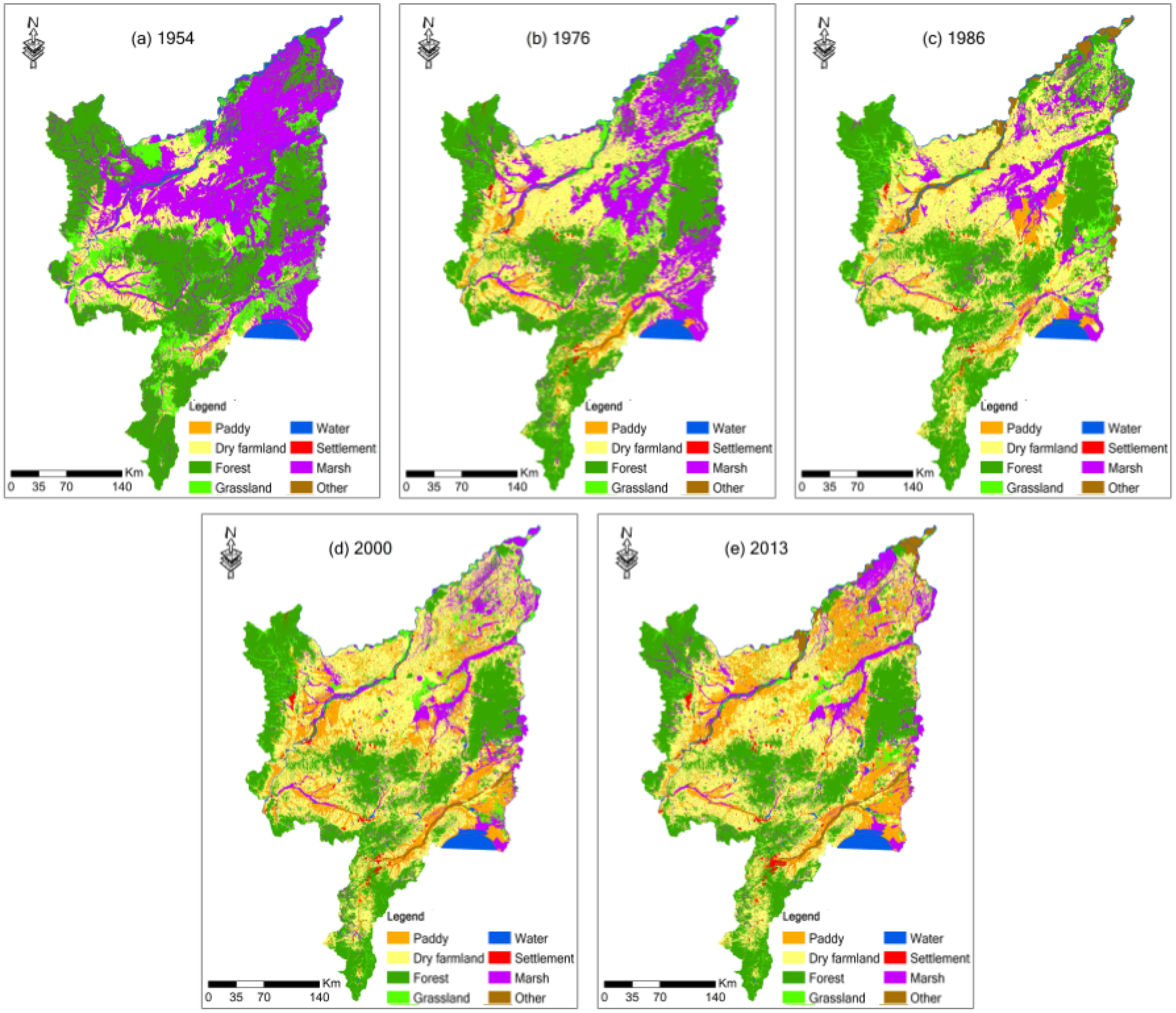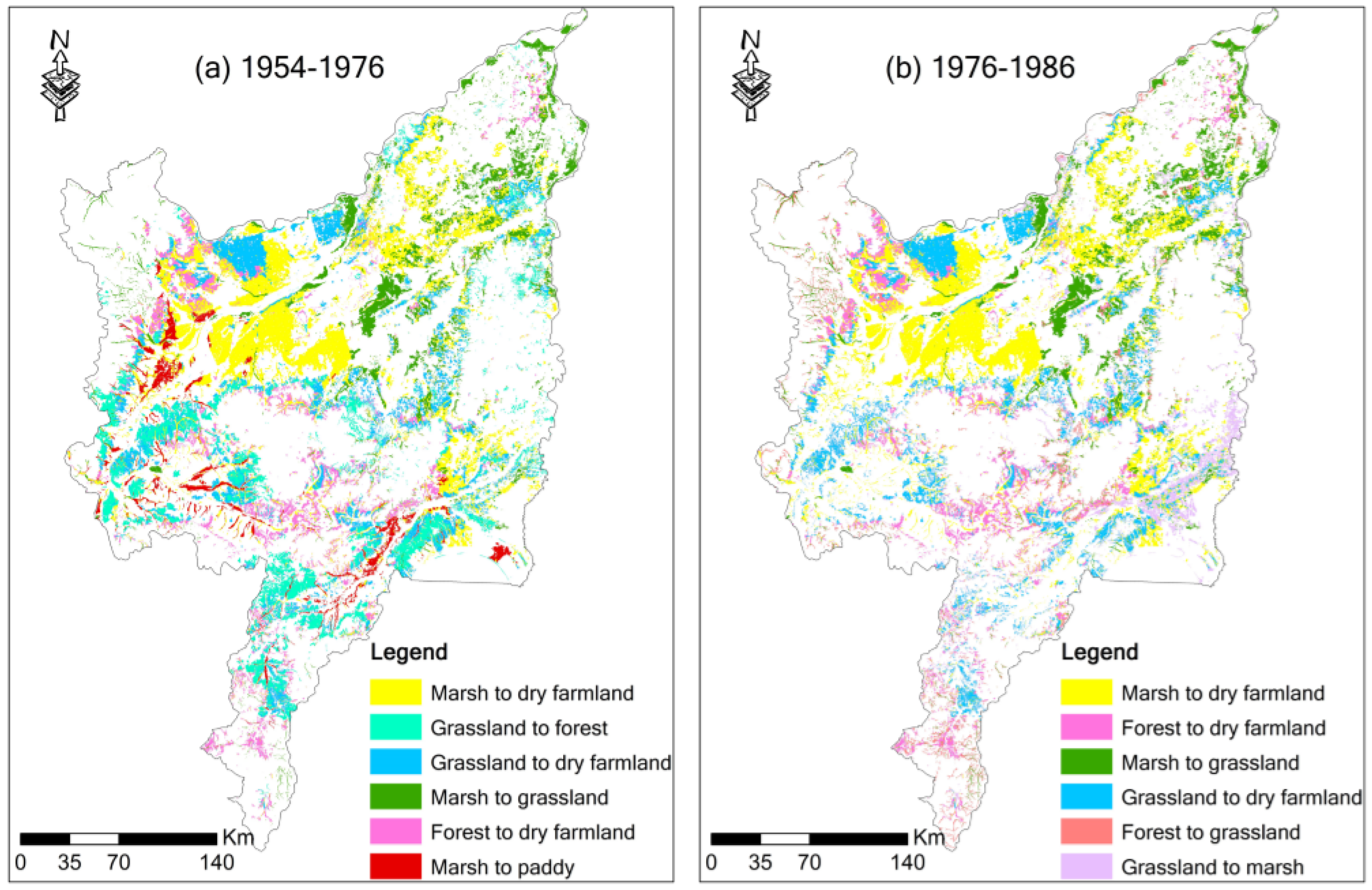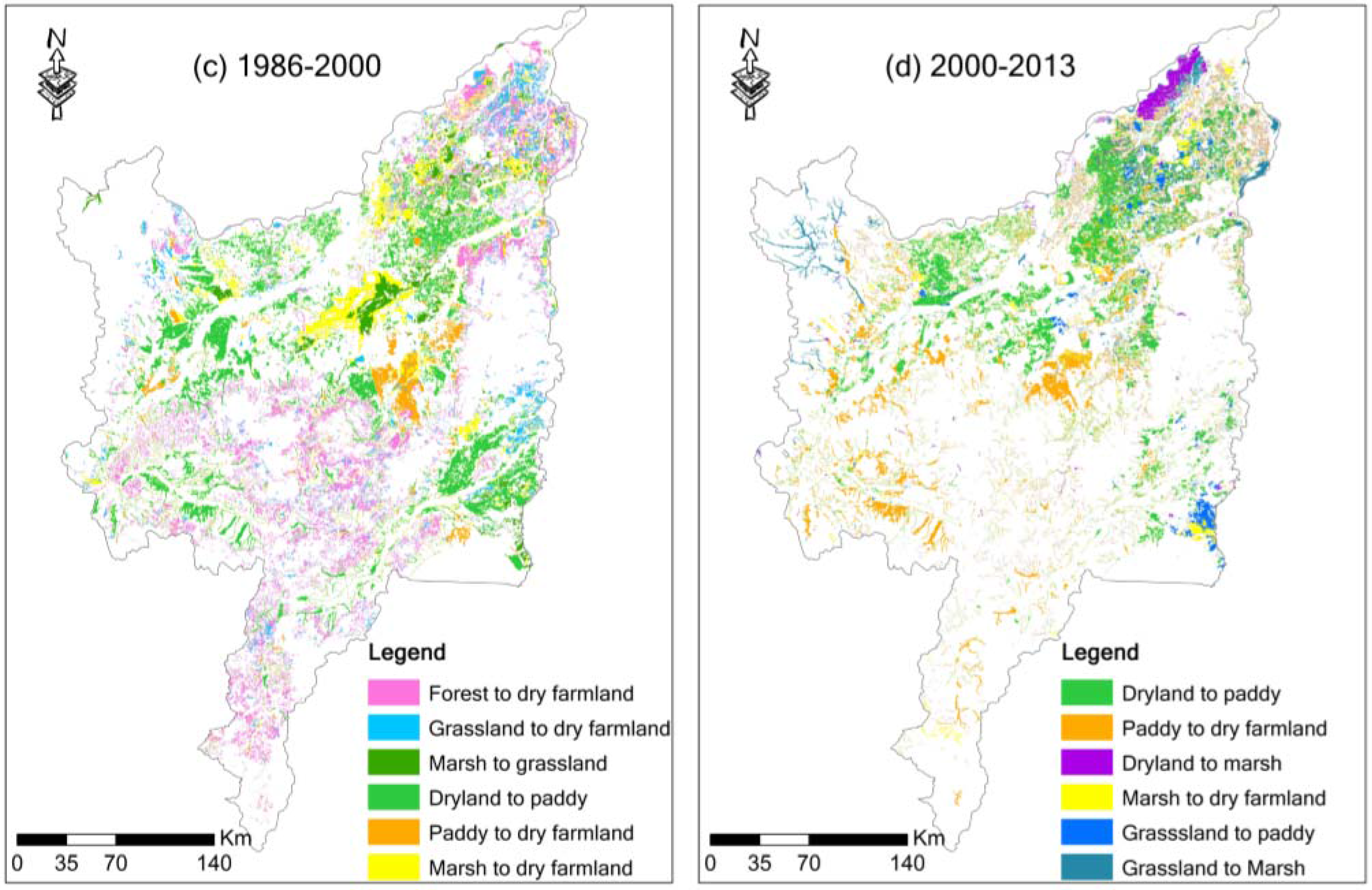One problem in estimating the accuracy of LULC classification is the lack of historical LULC data [9]. In this study, extensive field surveys were performed in the year 2000 and the year 2013 to ensure the accuracy of our maps. Meanwhile, historical records including aerial photos, tabular data in a large number of field sites and statistic data of Heilongjiang Province were used to estimate the interpretation results. Additionally, we interviewed many local people as well as experts to test the interpretation accuracy. In order to reduce error caused by post classification, the outline of LULCC is delimited by comparison of Landsat data in different periods. For example, the outline of LULC in 2000 is delimited by comparison of TM data in 1986 and 2000, with the references from land-use background in 1986. Even though they contain some uncertainties, the classification system and LULC maps reported by this study are credible.

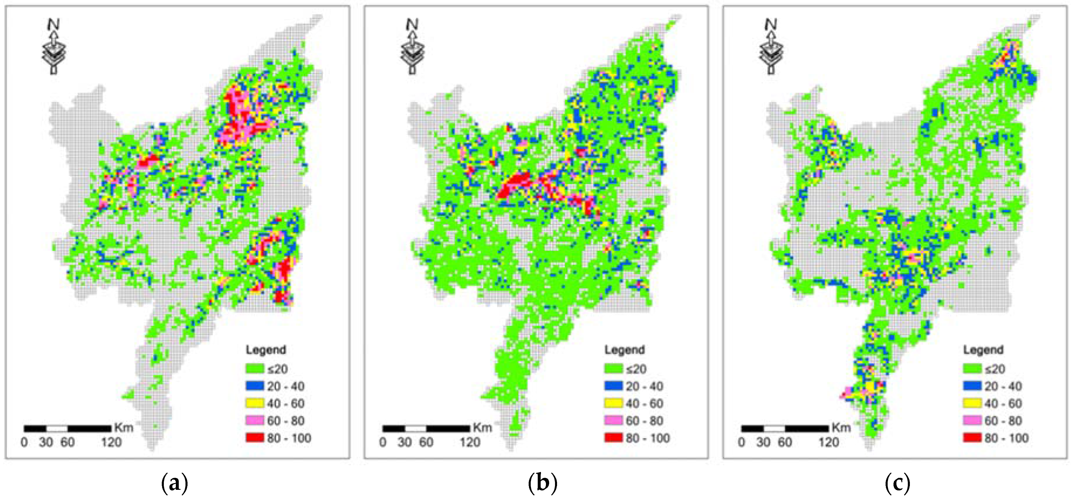
Human activities play a significant role in land degradation [56,57,58], and land degradation is particularly related to increases in population and intensive agriculture [64]. Our study showed that human activities (89.67%) were the dominant factors responsible for land degradation in the study area. In Sanjiang Plain, the population increased from 1.40 million in the 1950s to 9.74 million in the 2010s [56,62], which accounts for the growth of farmland and settlement area. Several other studies have also shown that population growth is an important factor in LULC. Government policies also had a substantial effect on the observed spatiotemporal changes in land degradation. In Sanjiang Plain, the “Great Leap Forward” movement [30,74] in the 1950s promoted the immigration of about 81,500 veterans to reclaim wetlands for farmland to produce more food [58]. Promoted by the “Going to the Countryside and Settling in the Communes” policy, approximately 450,000 educated youth moved to Sanjiang Plain and participated in agricultural activities in the early 1970s [9,58]. From 1978 to 1985, advanced agricultural machinery was introduced by the “Agricultural Modernization” [62] policy, promoting large-scale reclamation. From 1992 to 1995, the policy of “to promote conversion from dry farmland to paddy” in northeast China promoted conversion of dry farmland to paddy [75,76]. In the late 1990s, as the great ecological value of wetlands was recognized, the government began to take action to protect wetlands and some policies such as “returning farmland to wetland” were published [75,77,78] Additional, some policies such as "returning farmland to forestland", and "returning farmland to grassland" were put into place. All these policies affected the LULCC pattern in this region. The dramatic land degradation and the changes of land use structure that have taken place in this region will affect the water cycle, carbon balance and other biogeochemical processes. Future studies should investigate these questions.

The ESV estimation method used in this study was developed by Costanza et al. [31] and Xie et al. [47,48], and has been significant in estimating changes in ESV in response to human disturbance [34,79]. Based on NPP, we modified the value coefficients for the study area. The method used in this study was just one of many methods used to calculate ESV and the results are subject to some uncertainties such as limitations of economic valuation [31] and the possibility of double-counting [80,81]. As discussed in the Introduction, there are important differences between the ESV of paddy field and dry farmland. The trends in total ESV that we obtained were consistent with those from previous studies. However, our study captured a smaller ESV change between the 1980s and 2000s than previous studies. This result occurred mainly because we separated paddy and dry farmland in our study of ESV, whereas previous studies grouped paddy and dry farmland together as cropland. As a result, we captured ESV changes caused by the large changes in area from dry farmland to paddy during this period. We estimated the coefficients of these land use types using NPP and the coefficient cropland, which may include some degree of uncertainty. In the future, more accurate value coefficients for paddy and dry farmland are needed to produce better estimates of ESV. However, by estimating and comparing the ESV in different time periods in our study, uncertainties could be reduced or offset [34]. Additionally, our sensitivity analysis in our study indicated that our results are robust, despite these uncertainties.

Despite some shortcomings, ESV has the potential to provide policy-makers with scientifically sound information in order to achieve sustainable development. For example, C. Estoque et al. offered important insights for achieving more successful urban planning in an analysis of landscape and ESV change in Baguio City [51]. Based on analysis of ESV change in Chongming Island, Zhao et al. suggested that conservation of the wetlands and tidal flats should take precedence over the single-minded, uncontrolled reclamation of these areas for economic purposes in the future land use policies [23]. In this study, we found that the ESV decline caused by marsh and forest degradation decreased during 2000–2013 while the decline caused by grassland degradation was still severe. This result occurred mainly because the policies such as “returning farmland to wetlands”, ”returning farmland to wetland” and establishing reserves for wetlands in China limited the degradation of wetlands and forest to some extent. Therefore, the policy-makers should pay attention to changing other LULC types to grassland in addition to the protection of current grassland.

5. Conclusions

In the past 60 years, Sanjiang Plain has been significantly disturbed by human activities especially the large-scale reclamation. These activities have led to dramatic land degradation and major changes in land use structure. These changes also caused decreases in ecosystem service values and affected the structure of ecosystem services. Climate regulation and soil formation and protection were vulnerable to land degradation during the study period.

According to our analysis of ESV changes of different ecosystem functions, we found that the ESV of food production increased rapidly at the expense of almost all other ecosystem functions. If this trend continues, it will surely cause further deterioration of the ecological environment. Sensitivity analysis indicated that marsh ecosystems have the largest coefficient of sensitivity, followed by forest ecosystems. Since food production is no longer the most pressing concern in Sanjiang Plain, protecting current grassland, marsh and forest, and returning croplands to grassland, marsh and forest should be prioritized in the future.

References

1. Dewan, A.M.; Yamaguchi, Y.; Rahman, M.Z. Dynamics of land use/cover changes and the analysis of landscape fragmentation in Dhaka Metropolitan, Bangladesh. GeoJournal 2012, 77, 315–330. [Google Scholar] [CrossRef]
2. Dewan, A.M.; Yamaguchi, Y. Land use and land cover change in greater Dhaka, Bangladesh: Using remote sensing to promote sustainable urbanization. Appl. Geogr. 2009, 29, 390–401. [Google Scholar] [CrossRef]
3. Lambin, E.F. Modelling and monitoring land-cover change processes in tropical regions. Prog. Phys. Geogr. 1997, 21, 375–393. [Google Scholar] [CrossRef]
4. Gragson, T.L.; Bolstad, P.V. Land use legacies and the future of southern Appalachia. Soc. Nat. Resour. 2006, 19, 175–190. [Google Scholar] [CrossRef]
5. Lambin, E.F.; Turner, B.L.; Geist, H.J.; Agbola, S.B.; Angelsen, A.; Bruce, J.W.; Coomes, O.T.; Dirzo, R.; Fischer, G.; Folke, C. The causes of land-use and land-cover change: Moving beyond the myths. Glob. Environ. Chang. 2001, 11, 261–269. [Google Scholar] [CrossRef]
6. Dewan, A.M.; Yamaguchi, Y. Using remote sensing and GIS to detect and monitor land use and land cover change in Dhaka Metropolitan of Bangladesh during 1960–2005. Environ. Monit. Assess. 2009, 150, 237–249. [Google Scholar] [CrossRef] [PubMed]
7. Dewan, A.M.; Kabir, M.H.; Nahar, K.; Rahman, M.Z. Urbanisation and environmental degradation in Dhaka Metropolitan area of Bangladesh. Int. J. Environ. Sustain. Dev. 2012, 11, 118–147. [Google Scholar] [CrossRef]
8. DeFries, R.; Eshleman, K.N. Land-use change and hydrologic processes: A major focus for the future. Hydrol. Process. 2004, 18, 2183–2186. [Google Scholar] [CrossRef]
9. Wang, Z.; Zhang, B.; Zhang, S.; Li, X.; Liu, D.; Song, K.; Li, J.; Li, F.; Duan, H. Changes of land use and of ecosystem service values in Sanjiang Plain, Northeast China. Environ. Monit. Assess. 2006, 112, 69–91. [Google Scholar] [CrossRef] [PubMed]
10. Alves, D.S.; Skole, D.L. Characterizing land cover dynamics using multi-temporal imagery. Int. J. Remote Sens. 1996, 17, 835–839. [Google Scholar] [CrossRef]
11. Muttitanon, W.; Tripathi, N. Land use/land cover changes in the coastal zone of Ban Don Bay, Thailand using Landsat 5 TM data. Int. J. Remote Sens. 2005, 26, 2311–2323. [Google Scholar] [CrossRef]
12. Turner, B.L.; Lambin, E.F.; Reenberg, A. The emergence of land change science for global environmental change and sustainability. Proc. Natl. Acad. Sci. USA 2007, 104, 20666–20671. [Google Scholar] [CrossRef] [PubMed]
13. Foster, D.; Swanson, F.; Aber, J.; Burke, I.; Brokaw, N.; Tilman, D.; Knapp, A. The importance of land-use legacies to ecology and conservation. BioScience 2003, 53, 77–88. [Google Scholar] [CrossRef]
14. Chauchard, S.; Carcaillet, C.; Guibal, F. Patterns of land-use abandonment control tree-recruitment and forest dynamics in Mediterranean mountains. Ecosystems 2007, 10, 936–948. [Google Scholar] [CrossRef]
15. Zhou, Q.; Li, B.; Kurban, A. Trajectory analysis of land cover change in arid environment of China. Int. J. Remote Sens. 2008, 29, 1093–1107. [Google Scholar] [CrossRef]
16. Wang, D.; Gong, J.; Chen, L.; Zhang, L.; Song, Y.; Yue, Y. Comparative analysis of land use/cover change trajectories and their driving forces in two small watersheds in the western Loess Plateau of China. Int. J. Appl. Earth Obs. Geoinf. 2013, 21, 241–252. [Google Scholar] [CrossRef]
17. Mertens, B.; Lambin, E.F. Land-cover-change trajectories in southern Cameroon. Ann. Assoc. Am. Geogr. 2000, 90, 467–494. [Google Scholar] [CrossRef]
18. Wang, D.; Gong, J.; Chen, L.; Zhang, L.; Song, Y.; Yue, Y. Spatio-temporal pattern analysis of land use/cover change trajectories in Xihe watershed. Int. J. Appl. Earth Obs. Geoinf. 2012, 14, 12–21. [Google Scholar] [CrossRef]
19. Swetnam, R.D. Rural land use in England and Wales between 1930 and 1998: Mapping trajectories of change with a high resolution spatio-temporal dataset. Landsc. Urban Plan. 2007, 81, 91–103. [Google Scholar] [CrossRef]
20. Zhou, Q.; Li, B.; Kurban, A. Spatial pattern analysis of land cover change trajectories in Tarim Basin, northwest China. Int. J. Remote Sens. 2008, 29, 5495–5509. [Google Scholar] [CrossRef]
21. Bai, S.; Zhang, S. A study on the spatial-temporal land use conversion in county region–Taking Duerbete County as an example. J. Arid Land Resour. Environ. 2005, 1, 252–255. (In Chinese) [Google Scholar]
22. Yang, Y.; Zhang, S.; Wang, D.; Yang, J.; Xing, X. Spatiotemporal changes of farming-pastoral ecotone in Northern China, 1954–2005: A case study in Zhenlai County, Jilin Province. Sustainability 2014, 7, 1–22. [Google Scholar] [CrossRef]
23. Zhao, B.; Kreuter, U.; Li, B.; Ma, Z.; Chen, J.; Nakagoshi, N. An ecosystem service value assessment of land-use change on Chongming Island, China. Land Use Policy 2004, 21, 139–148. [Google Scholar] [CrossRef]
24. Isong, M.; Eyo, E.; Eyoh, A.; Nwanekezie, O.; Olayinka, D.N.; Udoudo, D.O.; Ofem, B. GIS cellular automata using artificial neural network for land use change simulation of Lagos, Nigeria. J. Geogr. Geol. 2012, 4, 94–101. [Google Scholar]
25. Lin, Y.P.; Chu, H.J.; Wu, C.F.; Verburg, P.H. Predictive ability of logistic regression, auto-logistic regression and neural network models in empirical land-use change modeling—A case study. Int. J. Geogr. Inf. Sci. 2011, 25, 65–87. [Google Scholar] [CrossRef] [Green Version]
26. Lin, Z.; Xia, B.; Dong, W. Analysis on temporal-spatial changes of land-use structure in Guangdong province based on information entropy. Trop. Geogr. 2011, 31, 266–271. [Google Scholar]
27. Henseler, M.; Wirsig, A.; Herrmann, S.; Krimly, T.; Dabbert, S. Modeling the impact of global change on regional agricultural land use through an activity-based non-linear programming approach. Agric. Syst. 2009, 100, 31–42. [Google Scholar] [CrossRef]
28. Huang, Y.; Xia, B.; Yang, L. Relationship study on land use spatial distribution structure and energy-related carbon emission intensity in different land use types of Guangdong, China, 1996–2008. Sci. World J. 2013, 2013, 1–15. [Google Scholar] [CrossRef] [PubMed]
29. Zheng, X.; Xia, T.; Yang, X.; Yuan, T.; Hu, Y. The land Gini coefficient and its application for land use structure analysis in China. PLoS ONE 2013, 8, e76165. [Google Scholar] [CrossRef] [PubMed]
30. Chen, L.; Wang, J.; Fu, B.; Qiu, Y. Land-use change in a small catchment of northern Loess Plateau, China. Agric. Ecosyst. Environ. 2001, 86, 163–172. [Google Scholar] [CrossRef]
31. Costanza, R.; d’Arge, R.; de Groot, R.; Faber, S.; Grasso, M.; Hannon, B.; Limburg, K.; Naeem, S.; O’neill, R.V.; Paruelo, J.; et al. The value of the world’s ecosystem services and natural capital. Nature 1997, 387, 253–260. [Google Scholar] [CrossRef]
32. Daily, G. Nature’s Services: Societal Dependence on Natural Ecosystems; Island Press: Washington, WA, USA, 1997. [Google Scholar]
33. Ouyang, Z.; Wang, R.; Zhao, J. Ecosystem services and their economic valuation. Chin. J. Appl. Ecol. 1999, 10, 635–640. (In Chinese) [Google Scholar]
34. Fei, L.; Shuwen, Z.; Jiuchun, Y.; Kun, B.; Qing, W.; Junmei, T.; Liping, C. The effects of population density changes on ecosystem services value: A case study in Western Jilin, China. Ecol. Indic. 2016, 61, 328–337. [Google Scholar] [CrossRef]
35. Brauman, K.A.; Daily, G.C.; Duarte, T.K.E.; Mooney, H.A. The nature and value of ecosystem services: An overview highlighting hydrologic services. Annu. Rev. Environ. Resour. 2007, 32, 67–98. [Google Scholar] [CrossRef]
36. Kozak, J.; Lant, C.; Shaikh, S.; Wang, G. The geography of ecosystem service value: The case of the Des Plaines and Cache River wetlands, Illinois. Appl. Geogr. 2011, 31, 303–311. [Google Scholar] [CrossRef]
37. Costanza, R.; Cumberland, J.H.; Daly, H.; Goodland, R.; Norgaard, R.B.; Kubiszewski, I.; Franco, C. An Introduction to Ecological Economics; CRC Press: Boca Raton, FL, USA, 2014. [Google Scholar]
38. Costanza, R.; Kubiszewski, I. The authorship structure of “ecosystem services” as a transdisciplinary field of scholarship. Ecosyst. Serv. 2012, 1, 16–25. [Google Scholar] [CrossRef]
39. Braat, L.C.; de Groot, R. The ecosystem services agenda: Bridging the worlds of natural science and economics, conservation and development, and public and private policy. Ecosyst. Serv. 2012, 1, 4–15. [Google Scholar] [CrossRef]
40. Peters, C.; Gentry, A.; Mendelsohn, R. Valuation of an Amazonian rainforest. Nature 1989, 339, 655–656. [Google Scholar] [CrossRef]
41. Pimentel, D.; Harvey, C.; Resosudarmo, P.; Sinclair, K.; Kurz, D.; McNair, M.; Crist, S.; Shpritz, L.; Fitton, L.; Saffouri, R. Environmental and economic costs of soil erosion and conservation benefits. Science 1995, 267, 1117–1122. [Google Scholar] [CrossRef] [PubMed]
42. Björklund, J.; Limburg, K.E.; Rydberg, T. Impact of production intensity on the ability of the agricultural landscape to generate ecosystem services: An example from Sweden. Ecol. Econ. 1999, 29, 269–291. [Google Scholar] [CrossRef]
43. Xie, G.; Zhen, L.; Lu, C.; Xiao, Y.; Chen, C. Expert knowledge based valuation method of ecosystem services in China. J. Nat. Resour. 2008, 23, 911–919. [Google Scholar]
44. Sherrouse, B.C.; Clement, J.M.; Semmens, D.J. A GIS application for assessing, mapping, and quantifying the social values of ecosystem services. Appl. Geogr. 2011, 31, 748–760. [Google Scholar] [CrossRef]
45. Xiao, Y.; Xie, G.; An, K. Economic value of ecosystem services in Mangcuo Lake drainage basin. J. Appl. Ecol. 2003, 14, 676–680. (In Chinese) [Google Scholar]
46. Rönnbäck, P. The ecological basis for economic value of seafood production supported by mangrove ecosystems. Ecol. Econ. 1999, 29, 235–252. [Google Scholar] [CrossRef]
47. Xie, G.; Lu, C.; Xiao, Y.; Zheng, D. The economic evaluation of grassland ecosystem services in Qinghai-Tibet plateau. J. Mt. Sci. 2003, 21, 50–55. [Google Scholar]
48. Xie, G.D.; Lu, C.X.; Leng, Y.F.; Zheng, D.; Li, S. Ecological assets valuation of the Tibetan Plateau. J. Nat. Resour. 2003, 18, 189–196. [Google Scholar]
49. Xie, G.D.; Xiao, Y.; Zhen, L.; Lu, C.X. Study on ecosystem services value of food production in China. Chin. J. Eco-Agric. 2005, 3, 10–13. (In Chinese) [Google Scholar]
50. Kreuter, U.P.; Harris, H.G.; Matlock, M.D.; Lacey, R.E. Change in ecosystem service values in the San Antonio area, Texas. Ecol. Econ. 2001, 39, 333–346. [Google Scholar] [CrossRef]
51. Estoque, R.C.; Murayama, Y. Landscape pattern and ecosystem service value changes: Implications for environmental sustainability planning for the rapidly urbanizing summer capital of the Philippines. Landsc. Urban Plan. 2013, 116, 60–72. [Google Scholar] [CrossRef]
52. Cen, X.; Wu, C.; Xing, X.; Fang, M.; Garang, Z.; Wu, Y. Coupling intensive land use and landscape ecological security for urban sustainability: An integrated socioeconomic data and spatial metrics analysis in Hangzhou city. Sustainability 2015, 7, 1459–1482. [Google Scholar] [CrossRef]
53. Wu, K.Y.; Ye, X.Y.; Qi, Z.F.; Zhang, H. Impacts of land use/land cover change and socioeconomic development on regional ecosystem services: The case of fast-growing Hangzhou metropolitan area, China. Cities 2013, 31, 276–284. [Google Scholar] [CrossRef]
54. Su, S.; Xiao, R.; Jiang, Z.; Zhang, Y. Characterizing landscape pattern and ecosystem service value changes for urbanization impacts at an eco-regional scale. Appl. Geogr. 2012, 34, 295–305. [Google Scholar] [CrossRef]
55. Ng, C.N.; Xie, Y.J.; Yu, X.J. Integrating landscape connectivity into the evaluation of ecosystem services for biodiversity conservation and its implications for landscape planning. Appl. Geogr. 2013, 42, 1–12. [Google Scholar] [CrossRef]
56. Song, K.; Liu, D.; Wang, Z.; Zhang, B.; Jin, C.; Li, F.; Liu, H. Land use change in Sanjiang Plain and its driving forces analysis since 1954. Acta Geogr. Sin. Chin. Ed. 2008, 63, 93–104. (In Chinese) [Google Scholar]
57. Song, K.; Wang, Z.; Du, J.; Liu, L.; Zeng, L.; Ren, C. Wetland degradation: Its driving forces and environmental impacts in the Sanjiang Plain, China. Environ. Manag. 2014, 54, 255–271. [Google Scholar] [CrossRef] [PubMed]
58. Wang, Z.; Song, K.; Ma, W.; Ren, C.; Zhang, B.; Liu, D.; Chen, J.M.; Song, C. Loss and fragmentation of marshes in the Sanjiang Plain, Northeast China, 1954–2005. Wetlands 2011, 31, 945–954. [Google Scholar] [CrossRef]
59. Zhou, D.; Gong, H.; Wang, Y.; Khan, S.; Zhao, K. Driving forces for the marsh wetland degradation in the honghe national nature reserve in sanjiang plain, northeast China. Environ. Model. Assess. 2009, 14, 101–111. [Google Scholar] [CrossRef]
60. Yan, M.H.; Deng, W.; Ma, X.H. Climate variation in the Sanjiang Plain disturbed by large scale reclamation during the last 45 years. Acta Geogr. Sin. Chin. Ed. 2001, 56, 170–179. [Google Scholar]
61. Wang, L.; Tian, H.; Song, C.; Xu, X.; Chen, G.; Ren, W.; Lu, C. Net exchanges of CO2, CH4 and N2O between marshland and the atmosphere in northeast China as influenced by multiple global environmental changes. Atmos. Environ. 2012, 63, 77–85. [Google Scholar] [CrossRef]
62. Liu, X.; Dong, G.; Wang, X.; Xue, Z.; Jiang, M.; Lu, X.; Zhang, Y. Characterizing the spatial pattern of marshlands in the Sanjiang Plain, northeast China. Ecol. Eng. 2013, 53, 335–342. [Google Scholar] [CrossRef]
63. Liu, H.; Zhang, S.; Li, Z.; Lu, X.; Yang, Q. Impacts on wetlands of large-scale land-use changes by agricultural development: The small Sanjiang Plain, China. AMBIO 2004, 33, 306–310. [Google Scholar] [CrossRef] [PubMed]
64. Liu, Y.; Peng, L.; Chen, Y. Conversion of land use types and ecological effect in Northeast China. Trans. Chin. Soc. Agric. Eng. 2005, 21, 175–178. (In Chinese) [Google Scholar]
65. Zhang, S.; Zhang, Y.; Li, Y.; Chang, L. Temporal Characteristics Analysis of Land Use/Land Cover in Northeast China; Science Press: Beijing, China, 2006. [Google Scholar]
66. Liu, J.; Liu, M.; Tian, H.; Zhuang, D.; Zhang, Z.; Zhang, W.; Tang, X.; Deng, X. Spatial and temporal patterns of China’s cropland during 1990–2000: An analysis based on Landsat TM data. Remote Sens. Environ. 2005, 98, 442–456. [Google Scholar] [CrossRef]
67. Liu, J.; Zhan, J.; Deng, X. Spatio-temporal patterns and driving forces of urban land expansion in China during the economic reform era. AMBIO 2005, 34, 450–455. [Google Scholar] [CrossRef] [PubMed]
68. Liu, J.; Zhang, Z.; Xu, X.; Kuang, W.; Zhou, W.; Zhang, S.; Li, R.; Yan, C.; Yu, D.; Wu, S. Spatial patterns and driving forces of land use change in China during the early 21st century. J. Geogr. Sci. 2010, 20, 483–494. [Google Scholar] [CrossRef]
69. Liu, J.Y.; Liu, M.L.; Deng, X.Z.; Zhang, D.F.; Zhang, Z.X.; Luo, D. The land use and land cover change database and its relative studies in China. J. Geogr. Sci. 2002, 12, 275–282. [Google Scholar]
70. Zhuang, D.; Liu, J.; Liu, M. Research activities on land-use/cover change in the past ten years in China using space technology. Chin. Geogr. Sci. 1999, 9, 330–334. [Google Scholar] [CrossRef]
71. Liu, J.; Liu, M.; Zhuang, D.; Zhang, Z.; Deng, X. Study on spatial pattern of land-use change in China during 1995–2000. Sci. China Ser. D Earth Sci. 2003, 46, 373–384. [Google Scholar]
72. Liu, J.; Tian, H.; Liu, M.; Zhuang, D.; Melillo, J.M.; Zhang, Z. China’s changing landscape during the 1990s: Large-scale land transformations estimated with satellite data. Geophys. Res. Lett. 2005, 32, 1–5. [Google Scholar] [CrossRef]
73. Bai, S.Y.; Zhang, S.W. The discussion of the method of land utilization spatial information reappearance of history period. J. Arid Land Resour. Environ. 2004, 18, 77–80. (In Chinese) [Google Scholar]
74. Verburg, P.H.; Bouma, J. Land use change under conditions of high population pressure: The case of Java. Glob. Environ. Chang. 1999, 9, 303–312. [Google Scholar] [CrossRef]
75. Seto, K.C.; Fragkias, M. Quantifying spatiotemporal patterns of urban land-use change in four cities of China with time series landscape metrics. Landsc. Ecol. 2005, 20, 871–888. [Google Scholar] [CrossRef]
76. Huang, N.; Liu, D.; Wang, Z. Study on mutual transformation characteristics between paddy field and dry land in Sanjiang Plain from 1986 to 2005. Resour. Sci. 2009, 2, 324–329. [Google Scholar]
77. Gong, P.; Niu, Z.; Cheng, X.; Zhao, K.; Zhou, D.; Guo, J.; Liang, L.; Wang, X.; Li, D.; Huang, H. China’s wetland change (1990–2000) determined by remote sensing. Sci. China Earth Sci. 2010, 53, 1036–1042. [Google Scholar] [CrossRef]
78. Huang, N.; Liu, D.; Wang, Z.; Zhang, B.; Song, K.S.; Ren, C.Y. Spatial decision analysis on returning farmland to wetland based on GIS in the Sanjiang Plain. Sci. Geogr. Sin. 2009, 29, 874–879. [Google Scholar]
79. Liu, Y.G.; Zeng, X.X.; Xu, L.; Tian, D.L.; Zeng, G.M.; Hu, X.J.; Tang, Y.F. Impacts of land-use change on ecosystem service value in Changsha, China. J. Cent. South Univ. Technol. 2011, 18, 420–428. [Google Scholar] [CrossRef]
80. Fu, B.J.; Su, C.H.; Wei, Y.P.; Willett, I.R.; Lü, Y.H.; Liu, G.H. Double counting in ecosystem services valuation: Causes and countermeasures. Ecol. Res. 2011, 26, 1–14. [Google Scholar] [CrossRef]
81. Konarska, K.M.; Sutton, P.C.; Castellon, M. Evaluating scale dependence of ecosystem service valuation: A comparison of NOAA-AVHRR and Landsat TM datasets. Ecol. Econ. 2002, 41, 491–507. [Google Scholar] [CrossRef]
Figure 1. The study area.
Remotesensing 08 00917 g001
Figure 2. Percentage of area of each land category, 1954–2013.
Remotesensing 08 00917 g002
Figure 3. (ae) LULCC maps in different periods.
Remotesensing 08 00917 g003
Figure 4. (ad) Main LULCC types in different stages.
Remotesensing 08 00917 g004aRemotesensing 08 00917 g004b
Figure 5. Spatial distribution of the transition probability index ( P i j t ) between 1954 and 2013 of different LULCC types (a) marsh to paddy; (b) Marsh to dry farmland; (c) forest to dry farmland; (d) grassland to dry farmland; (e) grassland to paddy; (f) dry farmland to paddy.
Remotesensing 08 00917 g005aRemotesensing 08 00917 g005b
Figure 6. Trajectories of LULCC, 1954–2013. (a) LULC change types with different steps; (b) Unchanged land; (c) Trajectory codes, 0 represents all other trajectory codes; (d) LULC change types.
Remotesensing 08 00917 g006
Figure 7. Lorenz curves of various LULC types.
Remotesensing 08 00917 g007
Figure 8. Gini coefficients for the different LULC types examined in this study from 1954 to 2013.
Remotesensing 08 00917 g008
Figure 9. DEM (a) and slopes (b) of Sanjiang Plain.
Remotesensing 08 00917 g009
Figure 10. R index values from 1954 to 2013.
Remotesensing 08 00917 g010
Figure 11. Changes in ecosystem services values.
Remotesensing 08 00917 g011
Figure 12. Effects of LULCC on percentage of ecosystem services values.
Remotesensing 08 00917 g012