Radiometric Resolution Analysis and a Simulation Model

Abstract

Total power radiometer has a simple configuration and the best theoretical resolution. Gain fluctuations and calibration errors, however, can induce severe errors in the solved scene brightness temperature. To estimate the overall radiometer performance we present a numerical simulation tool that can be used to determine the radiometric resolution. Our model considers three main components that degrade the radiometric resolution: thermal noise, 1/f noise and calibration errors. These error sources have long been known to exist, but comprehensive models able to account all these effects quantitatively and accurately in a practical manner have been missing. We have developed a radiometer simulation model that is able to produce radiometer signals that incorporate realistic radiometer effects that show up as noise and other errors in the radiometer video signal. Our simulation tool integrates the fundamental radiometer theories numerically and allows the investigation of different calibration schemes and receiver topologies. The model can be used as a guide for design and optimization as well as for verification of the radiometer performance. Moreover, it can be extended to a much larger and more complex radiometer systems allowing better system level performance estimation and optimization with minimal bread-board implementations. The model mimics real radiometer video data and thus the complete data analysis pipeline can be developed and verified before the real video data is available. In this paper, the model has been applied to a total power radiometer operating in the 52 GHz frequency range.

1. Introduction

Radiometers have been used in remote sensing to measure various properties related to the atmosphere and the surface of the Earth. The usual radiometer equation considering only the white noise and gain fluctuations reveals qualitative relations between the receiver noise power at the radiometer input, detection bandwidth, integration time and gain fluctuations, but is poorly suited to quantitative estimation of a total power radiometer resolution. Recent efforts [1] present a convenient modification to the ideal radiometer equation that account the errors from a cyclic calibration. This can be used to optimize the integration times and the calibration load temperatures with a given scene brightness temperature. However, the model neglects the receiver gain fluctuations which usually seriously degrade the radiometer resolution. In [2], the calibration errors and the gain fluctuations are considered analytically. Our approach considers the same underlying principles, but we describe an accessible simulation model where a time domain video signals are created for each measured load. These signals include the thermal noise as well as the receiver gain fluctuations. These time domain data streams are used to compute the radiometric resolution of an unknown scene. As such the model mimics real radiometer measurements. Moreover, the simulation tool is easily modifiable to different load and receiver configurations.

The paper is organized as follows: in Section 2 we describe the underlying theoretical principles and sources that determine the radiometer resolution. In Section 3 we present the instrumentation used for an example simulation and for the corresponding verification measurement. In Section 4 the developed simulation model is explained which is followed by an example simulation and a verification measurement in Section 5. Section 6 is the discussion and Section 7 concludes the paper.

2. Background

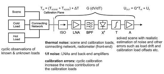
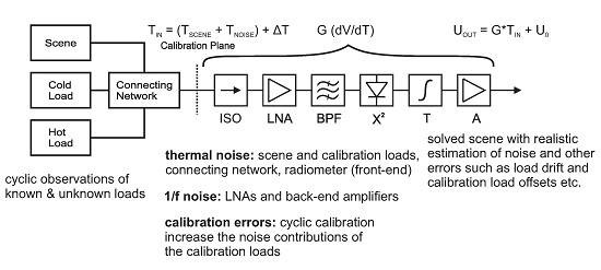
2.1. Total Power Radiometer

The output voltage of a total-power radiometer is a sum of a DC component and a time-varying fluctuation. The DC component is proportional to $T_{scene}+T_{noise}$. The measured voltage from the radiometer output and the radiometer input power are related by

$$U_{out}=G{\left(T_{scene}+T_{noise}\right)}^{\beta }+U_0$$

(1)

where $U_0$ is the combined offset of the video amplifier and the power detector, the gain of the radiometer is $G=kB\gamma G_{FE}A$ where k is the Boltzmann constant, B is the predetection bandwidth, $G_{FE}$ is the radiometer front-end gain, γ is the diode detector sensitivity and A is the video amplifier gain. The main source of offset is the video amplifier and the power detector. The $G{T}_{noise}$ term is not relevant here and therefore it can be sinked in the offset term $U_0$. Additionally, if we assume that the radiometer response is perfectly linear i.e., $\beta =1$, the Equation (1) reduces to

$$U_{out}=G{T}_{scene}+{\widehat{U}}_0$$

(2)

where ${\widehat{U}}_0=G{T}_{noise}+U_0$. Now we have two unknowns, the gain and the combined offset value ${\widehat{U}}_0$. Thus the needed amount of calibration points for a total power radiometer is two.

The standard deviation of the fluctuating part of the output voltage of a total power radiometer (after being reduced to the radiometer input) is the radiometric resolution $\Delta T$. According to [2] it consists of three terms:

• $\Delta T_S$, the thermal noise floor
• $\Delta T_G$, gain instability
• $\Delta T_C$, errors from the calibration

These three error sources jointly determine the obtainable radiometric resolution.

Total power radiometer can be considered as a cascade of the front-end (FE) and the back-end (BE) as shown in Figure 1. FE comprises an isolator, a low noise amplifier (LNA) and a band-pass filter (BPF). The FE provides sufficient gain for the detection as well as the frequency selectivity. The BE consists of a square law detector (X${}^2$) and a video amplifier (A) and it rectifies the high frequency signal to a DC signal. The video amplifier is used for the post detection amplification required before the analog-digital-converter (ADC). Both the FE and the BE contribute to the fluctuating part of the radiometer output via thermal noise and 1/f noise contributions.

When a radiometer is calibrated, it cyclically views calibration loads and a scene. Each of these measurements are affected by the noise created in the FE an BE in the same way. When these calibration measurements are used to solve the scene brightness temperature the radiometric resolution is degraded further due to the noise present in these calibration load measurements. This constitutes the term $\Delta T_C$.

We will discuss the noise contributions of the FE, BE and cyclic calibration to the radiometric resolution the remaining of this section.

Figure 1. Simplified total power radiometer block diagram.

Figure 1. Simplified total power radiometer block diagram.

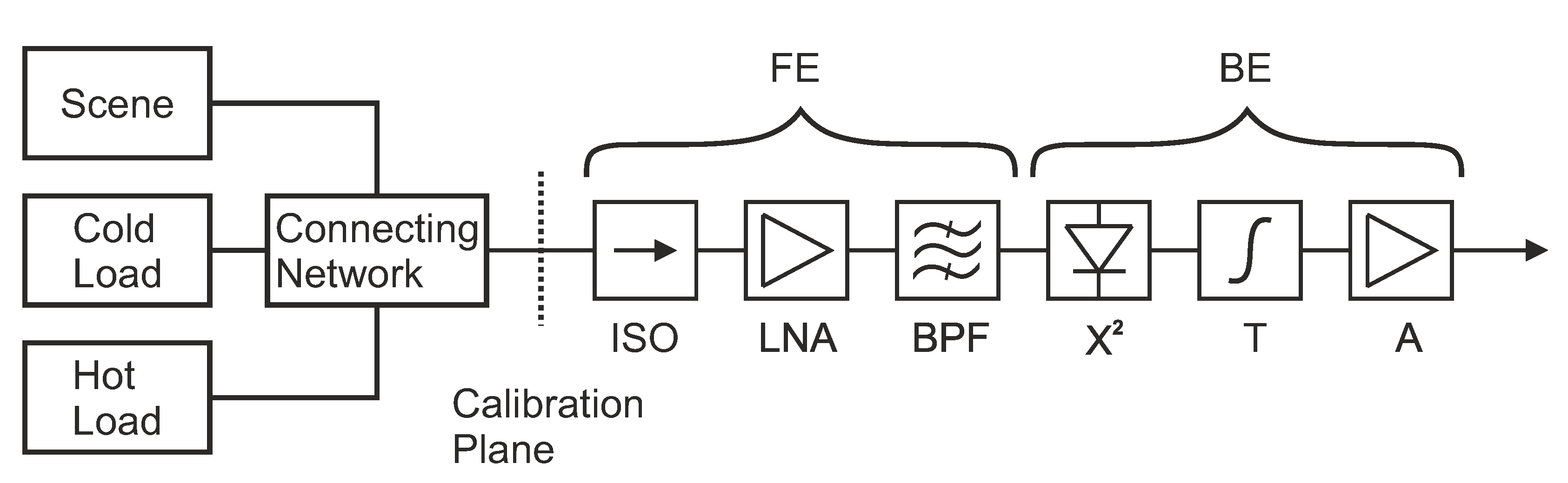
2.2. Noise Contribution of the FE

Radiometer noise (when one load is viewed) is usually modeled with two types of noise sources, white Gaussian distributed (non-correlated) and 1/f (correlated) noise [3]. These are caused by unrelated mechanisms and may be considered statistically independent. Therefore the practical radiometer equation is given by $\Delta T=\sqrt{\Delta T_{S,FE}^2+{(\Delta G_{FE}/G_{FE})}^2}$ which is a square root of the sum of variances of both noise components [4] where the non-correlated white noise in the total power radiometer FE is the commonly known ideal radiometric resolution

$$\Delta T_{S,FE}=\frac{T_{scene}+T_{noise}}{\sqrt{B\tau }}$$

(3)

where B is the pre-detection noise bandwidth and τ is the integration time of the video data. This equation gives the resolution of an ideal radiometer looking at the scene.

If the radiometer noise was white, the resolution could be improved indefinitely with longer integration times. In practice, the radiometer gain fluctuations, mainly arising from the LNA, hinder the ability to reduce the noise by integrating the video signal.

An empirical model describing the power spectral density (PSD) of the gain fluctuations is given in [5]. This model has a fixed PSD slope α, α = 1. We relax this assumption and allow α to have any value and then the PSD of the amplifier gain fluctuations reads

$$\frac{\Delta G_{FE}\left(f\right)}{G_{FE}}=\frac{2C\sqrt{N_S}}{f^{\alpha }}$$

(4)

where $N_S$ is the number of amplifier stages and C is a normalization constant. The normalization constant can vary considerably [5]. The model is only one possible alternative and others can be easily included to the model. Then the amplitude spectral density (ASD) of the FE noise contribution reduced to the radiometer input is

$$AS{D}_{FE}=\Delta T\left(f\right)=\left(T_{scene}+T_{noise}\right)\sqrt{\frac{1}{B}+{\left(\frac{\Delta G_{FE}\left(f\right)}{G_{FE}}\right)}^2}$$

(5)

2.3. Noise Contribution of the BE

The BE noise arises from the video amplifier noise and the thermal noise of the detectors internal resistance. To refer this noise, $v_n$, to the radiometer input we need to compute the radiometer gain G from the input brightness temperature to the video amplifier output voltage. Then the noise contribution from the BE reduced at the input of the radiometer can be expressed as

$$AS{D}_{BE}=\Delta T_{S,BE}=\frac{1}{\sqrt{2}}\frac{v_n}{G}$$

(6)

Here the $\sqrt{2}$ factor arises because $v_n$ is a one-sided spectral density. With a proper BE design with a low noise video amplifiers and a sufficient FE gain, the BE noise contribution is negligible. Additionally quantization noise of the analog-to-digital conversion contributes to the overall noise spectral density. The noise coming from the video amplifier, however, is usually several orders of magnitude higher than the quantization noise if a high resolution converter is used and thus the quantization noise can usually be omitted.

2.4. Noise Contribution of the Calibration Procedure

The limited resolution of the calibration load measurements degrades the overall radiometer resolution even if the calibration load brightness temperatures are ideally constant. Above we described how the radiometer resolution is affected by the random nature of the measured signal and the gain fluctuations when a scene is observed. These same limitations are present when the radiometer views the calibration loads. This measurement uncertainty leads the radiometer response to have an error in its slope and the error is different with consecutive calibration cycles [1]. Our simulation model incorporates this effect since the full calibration cycle with the known and unknown observations are included. This allows to determination of the optimal calibration load brightness temperatures for any scene brightness temperature.

3. Instrumentation

The radiometer is calibrated with two known calibration loads, a cryogenic load (CL) and a hot load (HL). These loads are connected to the radiometer through a lossy connecting network. We describe the uncertainty and stability of these loads and the effect of the connecting network in [6]. In the measurements and in the example simulation presented in this paper the scene is a matched load (ML) inside a temperature stabilized radiometer box with a set brightness temperature of $T_{ML}$ = 300.15 K.

A simplified block diagram of the radiometer is shown in Figure 1. The LNA block has 3 LNA chips and each of them contain three transistors. The radiometer center frequency is 52 GHz and the bandwidth is 4.2 GHz. Before the radiometer can be calibrated all noise sources need to be referenced to the calibration plane. The solved scene is then also given at the calibration plane from where it needs to be converted to the scene terminals. We describe these conversions in [6] and here we only consider the analysis at the calibration plane.

4. Simulation Model

4.1. Simulation Model Steps

• Generate one long block of a radiometer video signal including the FE and the BE noise contributions at the calibration plane with a specific integration time τ.
• Generate a video signal for each load that the radiometer views cyclically from the above generated long video signal with a brightness temperature offset that presents a specific load. The result is a set of cycles where each cycle contain one averaged brightness temperature estimate for each measured load.
• Solve the unknowns from above determined cycle using the information derived from the known calibration load video signals. One scene brightness temperature estimate is obtained from each cycle. The result is a time stream of a solved scene brightness temperatures with a specified τ.

4.2. Radiometer Video Signal

Our radiometer simulation requires realizations of the time-domain video signals for each load that the radiometer views. ADS’s of the radiometer FE and BE were given earlier in this paper (Equations (5) and (6)). Both ASD’s are referenced to the radiometer input.

First a time-domain noise signal realization that corresponds a given spectrum was generated. The spectrum bin amplitudes of each frequency bin were multiplied with an independent zero-mean complex Gaussian random variable of unit variance. Then an inverse-FFT of the randomized spectrum was computed and the real part was taken which is the time-domain noise signal realization. Using this approach and assuming a fixed load noise temperature we computed long time domain realizations of the FE and BE spectra. The lengths of the sequences represented the entire time of the simulated measurement session including all loads which are measured consecutively.

To represent the actual viewed loads during the measurement cycle we rescaled the subsections of the FE noise and added offsets to match each subsections overall noise temperature to the $T_{load}+T_{noise}$. This was achieved by adding first an offset of 290 K + $T_{noise}$ to the FE noise signal realization. Then the FE sequence was multiplied with ($T_{load}$ + $T_{noise}$)/(290 K + $T_{noise}$) to adjust the level of the offset and the noise correctly for each load with different brightness temperature. Finally we added the resulting sequence to the BE noise sequence which had zero offset. This signal presents the radiometer signal reduced to the input of the radiometer. When the data needs to be referenced to the output of the radiometer, it is multiplied with radiometer G.

The raw FE and BE noise sequences were generated with a sampling rate that was significantly larger than the integration times considered in the radiometer. In the simulation the raw sequences were averaged to the required integration time before they were applied in the data post-processing.

4.3. Cyclic Observations

The radiometer views cyclically three loads: CL, HL and Scene. The CL and the HL are known calibration loads and the scene is unknown. This measurement cycle has three possible observations. There is two known brightness temperatures $T_{hot}$ and $T_{cold}$ and one unknown $T_{scene}$. There are three unknowns to be solved from the radiometer observations: the radiometer gain G, the offset ${\widehat{U}}_0$ and the brightness temperature $T_{scene}$. Each measured load is averaged over the load dwell time. Therefore we have three measured observations for each cycle which are denoted as $U_1\dots U_3$.

In the observations the $T_{scene}$ is multiplied with the unknown gain G. Therefore a new variable has to be defined to keep the system linear as $U_{scene}=G{T}_{scene}$. The unknowns are solved first and then the brightness temperature $T_{scene}$ is obtained by dividing it with the solved gain estimate. The calibration equations can be presented in the following compact form:

$$\overline{u}=\left(\begin{array}{c}{U}_1\\ U_2\\ U_3\end{array}\right)=\left(\begin{array}{ccc}{T}_{hot}& 1& 0\\ T_{cold}& 1& 0\\ 0& 1& 1\end{array}\right)\left(\begin{array}{c}G\\ {\widehat{U}}_0\\ U_{scene}\end{array}\right)=M\overline{b}$$

(7)

The vector $\overline{u}$ contains the measured voltages and the vector b contains the unknowns. These vectors together with the matrix M determine the system.

5. Results

5.1. Simulation Model Parameter Extraction

We validated our simulation model by performing a 97-h test. All measured brightness temperatures were converted to the radiometer input i.e., to its calibration plane [6]. We make the comparison between the simulation and the measurement at this plane. To verify the model and discount any discrepancy arising from the erroneous input parameter estimation, we measured all parameters of our instruments required for the simulation that corresponds the verification measurement. All parameters used for the simulation are presented in Table 1.

Table 1. Parameters used in the simulation. The type refers to whether or not the parameter is known to the simulator. the brightness temperatures are given at the calibration plane of the radiometer.

Parameter	Value	Type
T${}_{hot}$	342 K	known by design
T${}_{cold}$	110 K	known by design
T${}_{scen{e}^{*}}$	300 K	unknown and solved
G${}^{*}$	1.44 mV/K	unknown and solved
U${}_0$	0	unknown and solved
T${}_{noise}$	670 K	known by measurement
B	4.2 GHz	known by measurement
C	0.73e-5	known by measurement
N${}_s$	9	known by design
α	1.0916	known by measurement
A	961	known by design
$v_n$	8 nV/rtHz	known by measurement
τ	200 s	known by design

Table 1. Parameters used in the simulation. The type refers to whether or not the parameter is known to the simulator. the brightness temperatures are given at the calibration plane of the radiometer.

Parameter	Value	Type
T${}_{hot}$	342 K	known by design
T${}_{cold}$	110 K	known by design
T${}_{scen{e}^{*}}$	300 K	unknown and solved
G${}^{*}$	1.44 mV/K	unknown and solved
U${}_0$	0	unknown and solved
T${}_{noise}$	670 K	known by measurement
B	4.2 GHz	known by measurement
C	0.73e-5	known by measurement
N${}_s$	9	known by design
α	1.0916	known by measurement
A	961	known by design
$v_n$	8 nV/rtHz	known by measurement
τ	200 s	known by design

5.1.1. Calibration Load Parameters

The brightness temperatures of the calibration loads are known by design and are used as such as known values. The $T_{scene}$ is solved from the measurement and is used as an input value for the simulator. This is not told to the simulator and it is solved as unknown. Similarly, the G and ${\widehat{U}}_0$ are solved from the measurement and used as input values in the verification simulation (again the values are not told to the simulator).

5.1.2. FE Parameters

The thermal noise model parameters $T_{noise}$ and B are required to estimate the white noise contribution of the FE. These were measured with a network analyzer without the diode detector. We do not expect the diode detector to deviate the measured results as it has significantly wider bandwidth than the radiometer and the FE noise is determined by the LNAs.

The gain fluctuation model requires only two parameters for defining the radiometer PSD. We placed a matched load at the input of the radiometer and recorded the radiometer video signal. Then the video signal was reduced to the radiometer input by dividing it by the radiometer gain G. From this data we computed the ASD with an FFT and extracted the parameters C and α. The measured ASD and the resulting model fit is shown in Figure 2a. Our averaged sample frequency was 1 Hz and therefore the white noise contribution as well as the knee frequency (1/f and white noise have equal power spectral densities) is not visible although it is included in the model as explained in Section 2. The extracted parameters can then be plugged into the $AS{D}_{FE}$ (Equation (5)).

5.1.3. BE Parameters

By measuring the BE stage (diode detector + video amplifier) individually an estimate for the white noise spectral density of the BE $v_n=8$$nV/\sqrt{Hz}$ was obtained. Reducing this noise to the input of the radiometer revealed that the FE noise contribution is significantly larger and the BE has negligible impact on the overall performance.

5.1.4. Integration Time

The same video signal measurement that was used to compute the PSD and extract the gain fluctuation parameters was used for the Allan deviation computation as well. The Allan deviation measurement and the simulation comparison is shown in Figure 2b. The Allan deviation is descending at small integration times which is a result of the white noise floor dominance at the high frequencies of the spectrum. This is not shown in the figure due to 1 Hz sample frequency. The slightly increasing part is a result of 1/f noise. Since the PSD slope is larger than 1 (ASD slope larger than 0.5) the Allan deviation is increasing at larger integration times. We can see a clear increase in the Allan deviation at about 1000 s. If we model the PSD with a simple straight line (in log-log scale) we are unable to predict this increase. However, we are not restricted to any particular shaped PSD. It is clear from the video signal measurement that at lower frequencies the PSD slope is clearly increasing. A step-wise fit of the measured PSD (Figure 2a) leads to a correct prediction of the Allan deviation at longer integration times as well.

Figure 2. (a) Amplitude spectral density of the radiometer noise. The noise represents 300 K scene brightness temperature. Note that the noise spectra are referred to the input of the radiometer (to its calibration plane); (b) Allan deviation of the radiometer video signal reduced to the input of the radiometer. τ is the integration time of the video signal.

Figure 2. (a) Amplitude spectral density of the radiometer noise. The noise represents 300 K scene brightness temperature. Note that the noise spectra are referred to the input of the radiometer (to its calibration plane); (b) Allan deviation of the radiometer video signal reduced to the input of the radiometer. τ is the integration time of the video signal.

We chose a dwell time for each load to be 200 s. The dwell time presents a single measurement of a particular load and thus the integration time is 200 s. We use this for the simulation and for the measurement when we investigate the radiometric resolution with full cyclic calibration. In our chosen integration time the Allan deviation is not yet strongly increasing and both simple linear fit as well as the step wise fit result in a similar radiometric resolution predictions.

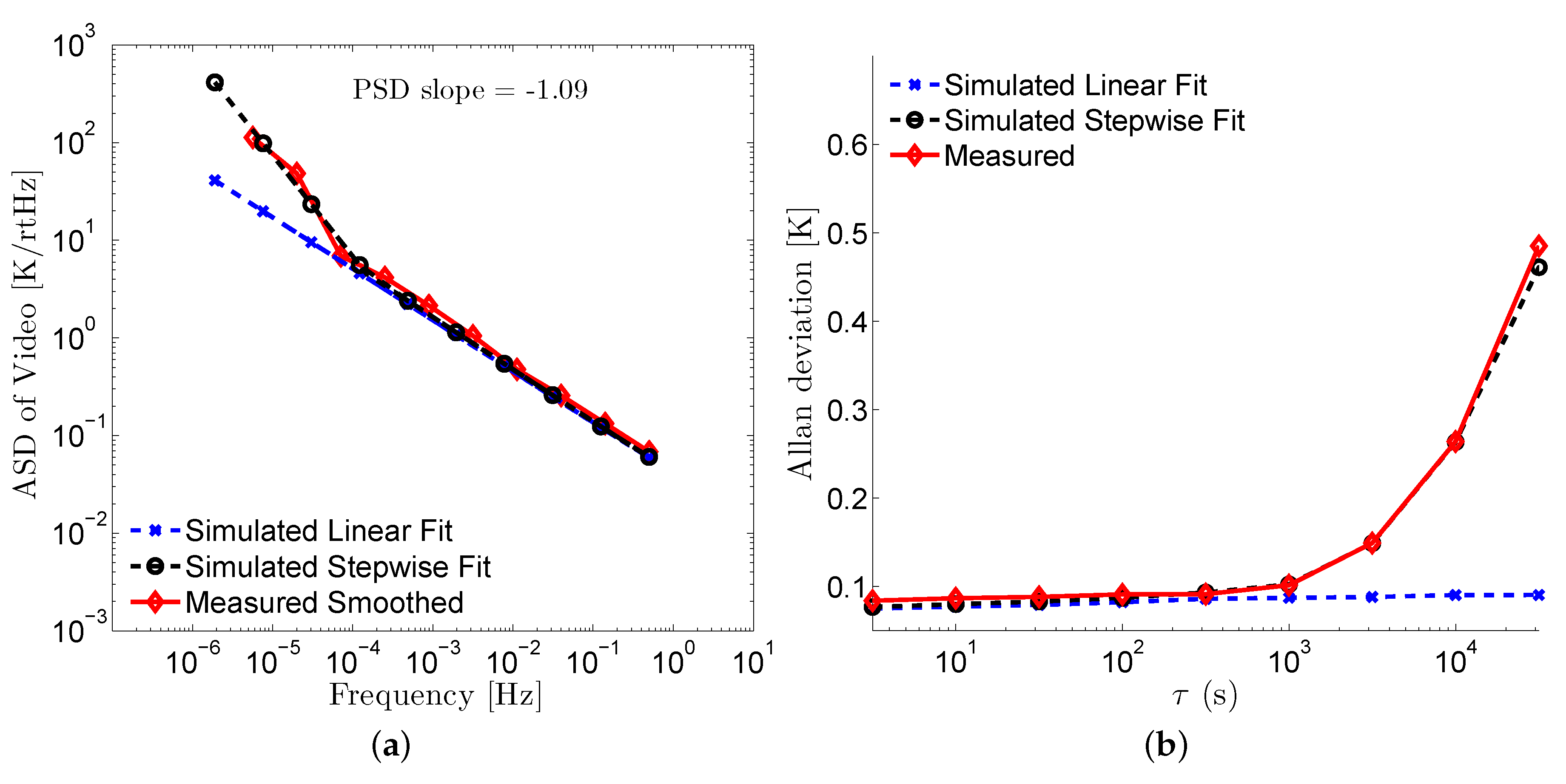
5.2. Radiometric Resolution

The radiometer can only be calibrated when the cryogenic load is cooled. Our load has a cool time period of about 5 h. Cool-down was done once per working day during the validation test. The cool-down allowed us to solve all three unknowns.

In Figure 3 we show the simulated and the measured solved $T_{scene}$. In the simulation we have solved the resolution for entire duration of the simulation. This simply yields more data points in the simulation compared to the measurement. Computing the resolution from both data sets reveal a good agreement between the simulation and the measured values in the same setup. The nominal brightness temperature estimation is practically perfect. The simulation and measurement radiometric resolution are in good agreement with ${\sigma }_{ML}$ = 0.158 K and 0.144 K respectively. The calibration loads have small, but known, drift in them and the number of samples varies between different cryogenic load cool-downs. Therefore we solved the experimental radiometric resolution using a standard deviation where the mean was independently computed for each cool-down.

Figure 3. Simulated (a) and measured (b) radiometer brightness temperatures and the corresponding resolutions. The scene is a temperature stabilized matched load. The brightness temperature and the resolution is solved for entire 97 h in the simulation. In the measurement it is solved during the five cryogenic load cool-downs, each lasting about five hours.

Figure 3. Simulated (a) and measured (b) radiometer brightness temperatures and the corresponding resolutions. The scene is a temperature stabilized matched load. The brightness temperature and the resolution is solved for entire 97 h in the simulation. In the measurement it is solved during the five cryogenic load cool-downs, each lasting about five hours.

6. Discussion

We presented an approach to estimate the overall resolution of a total power radiometer video signal. Our approach integrates the effect of the white noise, 1/f noise and the error induced by the calibration into a convenient numerical simulation tool. We showed an example simulation for the radiometric resolution when a temperature stabilized matched load was viewed. By measuring our radiometer FE and BE separately we were able to extract all parameters required for the simulation. The simulated radiometer performance agrees well with the measured results. However, if all parameters, especially the 1/f performance is not known, estimates need to be used in the simulation. Simulation based on estimates from [5] ($C=2E-5$ and α = 1) predicts resolution of 0.307 K, more than double than the measured due to the over estimation of the normalization constant. If one were to include only calibration errors and white noise, the resolution is about two orders of magnitude better than measured. Calibration error increases the resolution prediction approximately by half compared to the ideal radiometer equation. The simulation shows that the commonly used ideal radiometer equation is only suitable for qualitative prediction of the radiometer performance.

Many radiometer parameters are difficult to predict purely by theory and thus the model is partly based on theoretical assumptions and measurement results. The LNA 1/f noise degrades the radiometer resolution significantly and is particularly difficult to estimate. A theoretical model has been proposed in [5] but it also contains an amplifier specific normalization constant that can vary significantly. Additionally the 1/f slope variation of the LNAs have a strong impact on the radiometer resolution which is difficult to predict for a particular LNA without measuring it. Only two parameters, however, are required to model the noise characteristics of the LNAs. The used model is flexible and it can be updated with an appropriate measurement results when they become available to have more accurate system performance simulation.

7. Conclusions

We developed a model able to estimate the overall resolution and performance of a total power radiometer video signal. Our approach integrates the effect of white and 1/f noise as well as the errors induced by the calibration into a convenient numerical simulation tool. Previous attempts have dealt with extending the ideal radiometer equation to include the calibration errors [1], but omitted gain fluctuations which are the most prominent factor determining the obtainable resolution. Gain fluctuations are included in [2] with a cyclic calibration, but the approach is not flexible nor easily extendable for larger and more complex radiometer systems. Models able to produce realistic signals flexibly on different receiver and calibration load configurations has not been developed before. Our radiometer simulation model produces realistic radiometer video signals which can predict the overall radiometer performance. The model mimics real radiometer video data and thus the complete data analysis pipeline can be developed and verified before the real video data is available. We incorporated the essential noise sources and calibration errors. The tool, however, is not limited to these sources of error and e.g., drifts in calibration loads and offset errors are easily included. The model can be used for design optimization and performance evaluation of the radiometer and it is modifiable to any calibration load or receiver configuration as long as the underlying theoretical principles remain the same. It is expected that using the presented tool the time and the cost of a radiometer design can be significantly reduced. The benefit is even greater for larger and more complex systems since the minimization of hardware prototyping has greater impact.

References

1. Racette, P.; Lang, R.H. Radiometer design analysis based upon measurement uncertainty. Radio Sci. 2005, 40. [Google Scholar] [CrossRef]
2. Hersman, M.S.; Poe, G.A. Sensitivity of the total power radiometer with periodic calibration. IEEE Trans. Microw. Theory Tech. 1981, 29, 32–40. [Google Scholar] [CrossRef]
3. Poutanen, T. Map-Making and Power Spectrum Estimation for Cosmic Microwave Background Temperature Anisotropies. Ph.D Thesis, University of Helsinki, Helsinki, Finland, 2005. [Google Scholar]
4. Ulaby, F.T.; Moore, R.K.; Fung, A.K. Microwave Remote Sensing: Active and Passive; Artech House: Norwood, MA, USA, 1981; Volume 1. [Google Scholar]
5. Seiffert, M.; Mennella, A.; Burigana, C.; Mandolesi, N.; Bersanelli, M.; Meinhold, P.; Lubin, P. 1/f noise and other systematic effects in the Planck-LFI radiometers. Astrophysics 2002. [arXiv:astro-ph/0206093]. [Google Scholar] [CrossRef]
6. Kaisti, M.; Altti, M.; Poutanen, T. Uncertainty of radiometer calibration loads and its impact on radiometric measurements. IEEE Trans. Microw. Theory Tech. 2014, 62, 2435–2446. [Google Scholar] [CrossRef]