
Real-Time Classification of Seagrass Meadows on Flat Bottom with Bathymetric Data Measured by a Narrow Multibeam Sonar System

Abstract
:
1. Introduction
2. Materials and Methods
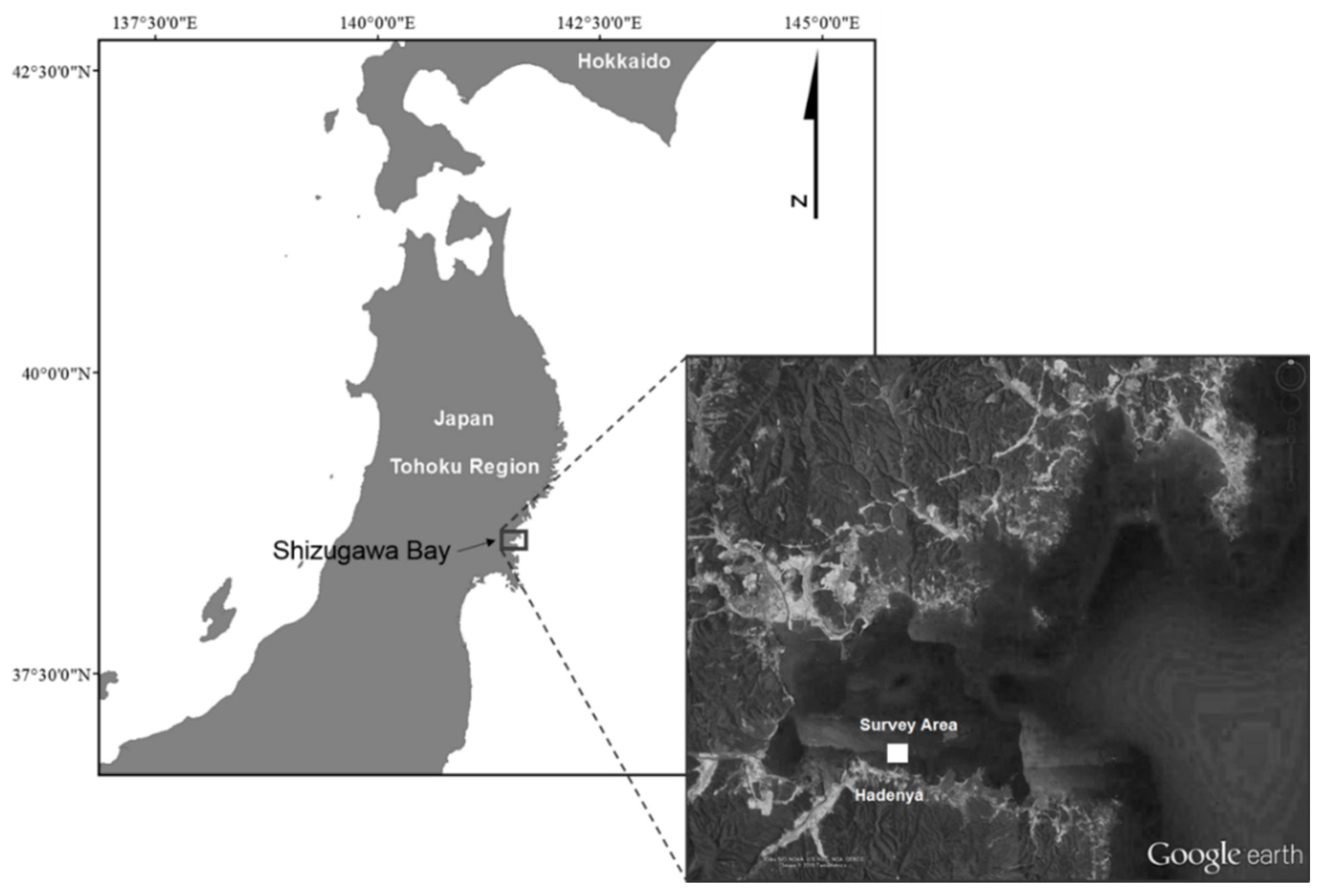
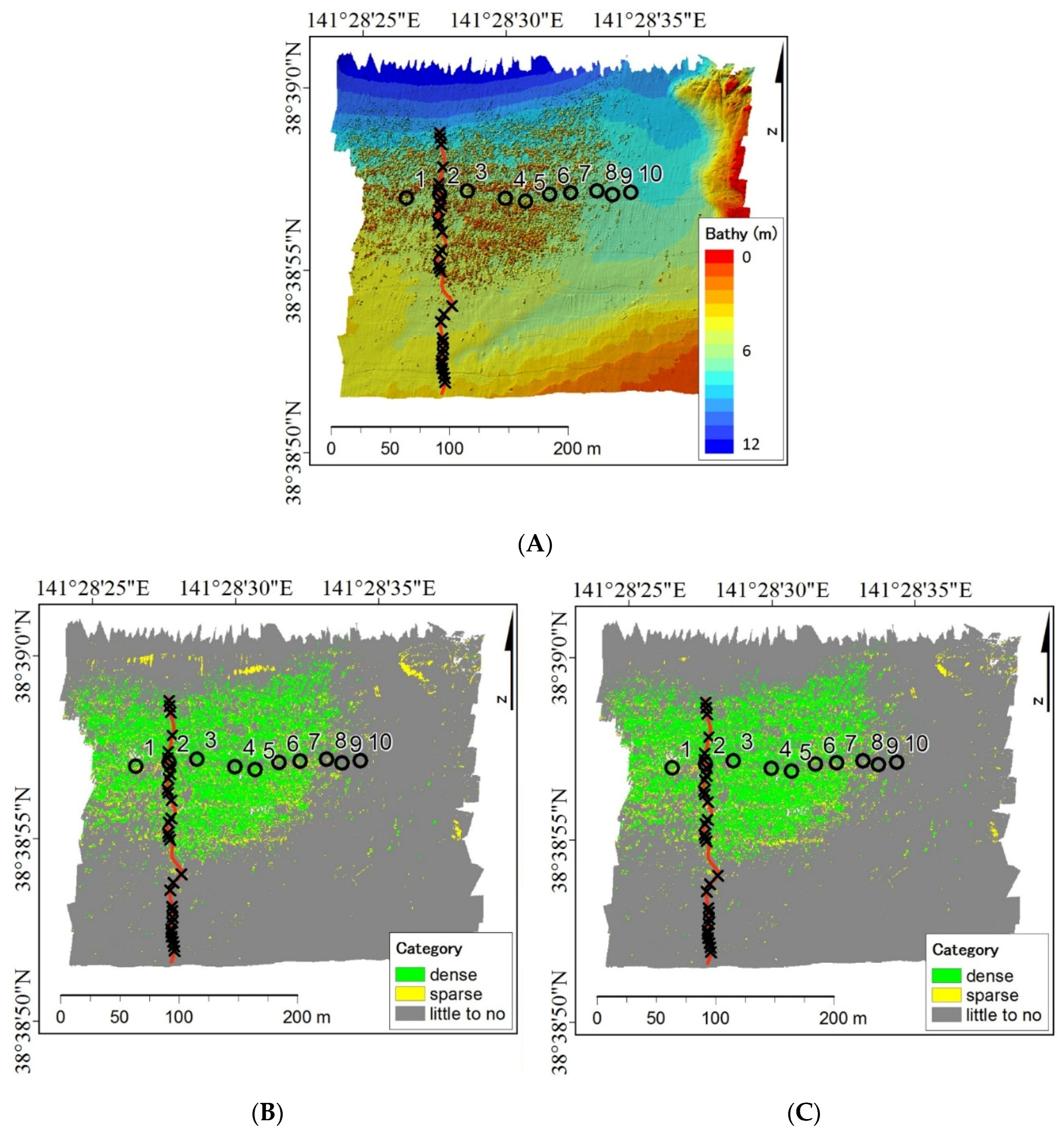
2.1. Survey Area

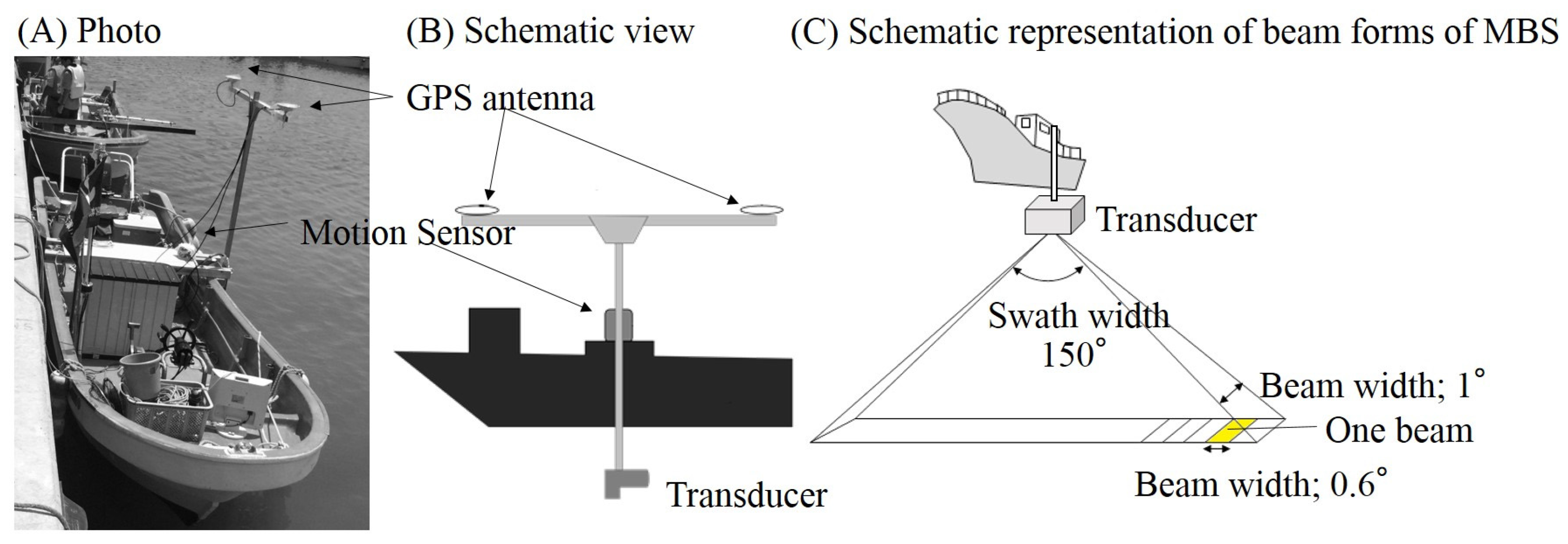
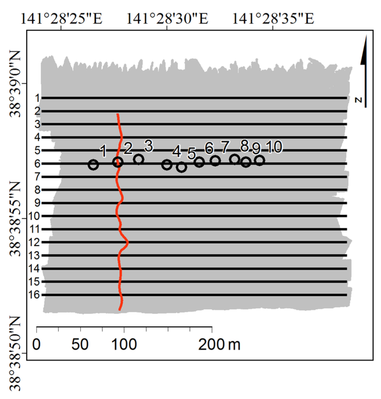
2.2. Data Acquisition


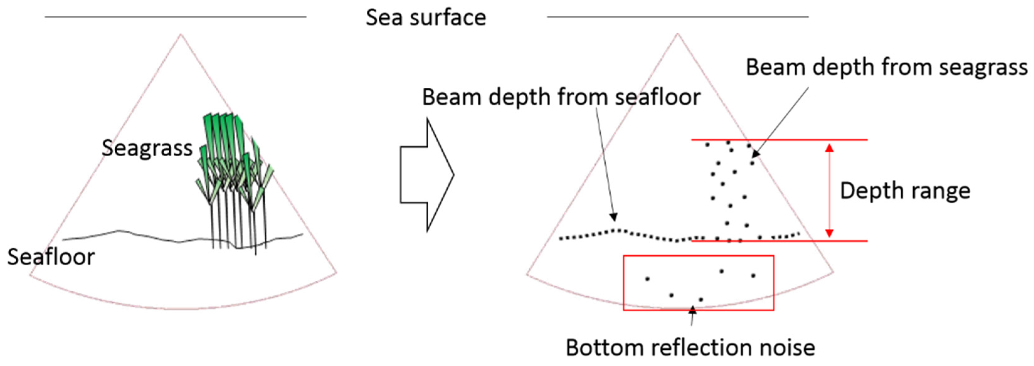
2.3. Data Analysis

3. Results
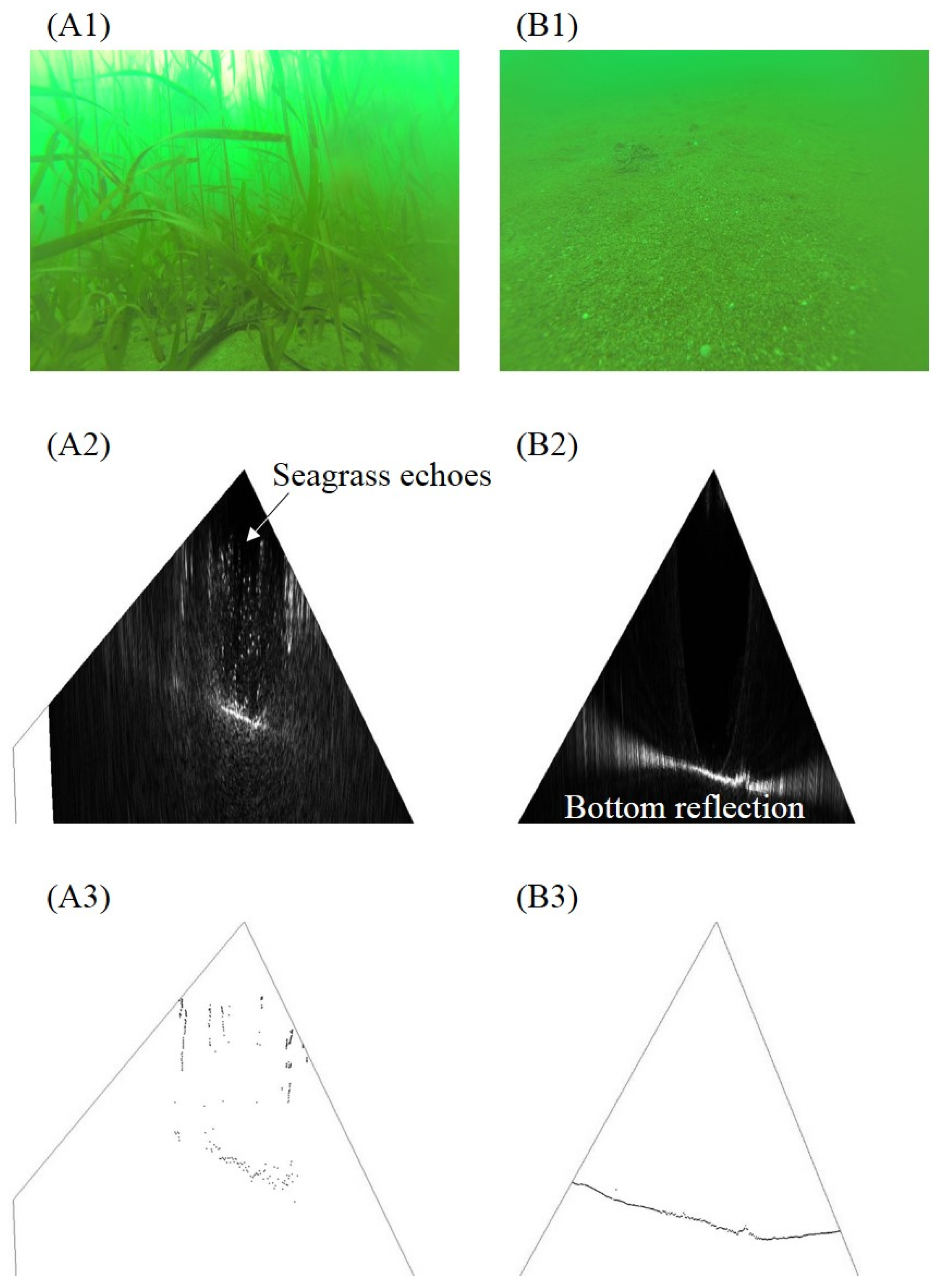
3.1. Comparison of Water Column Acoustic Images (WCIs) with the Underwater Images

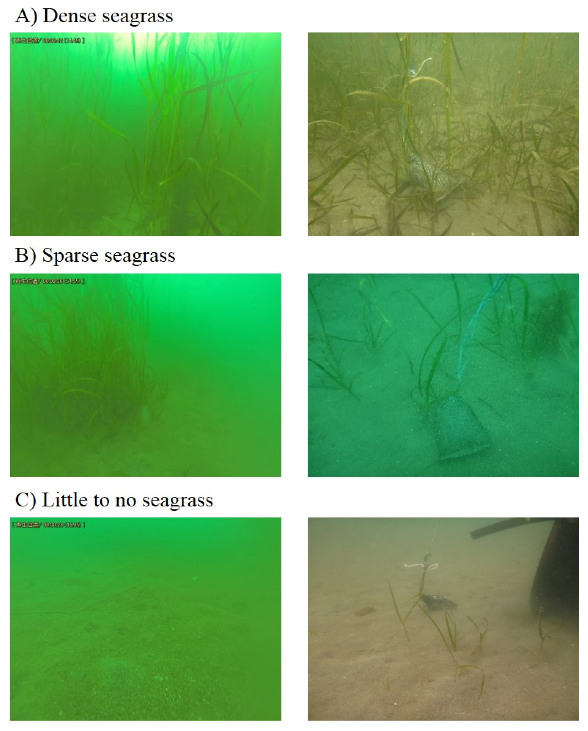
3.2. Classification of Stations into Three Categories of Seagrass Relative Abundance


| Underwater Photo | Acoustic Data (Beam Depth) | |||||
|---|---|---|---|---|---|---|
| Categories | Stns. | 95% Confidence Level | Depth Range (m) | Mean Bottom Depth (m) | ||
| Mean | S.D. | Mean | S.D. | |||
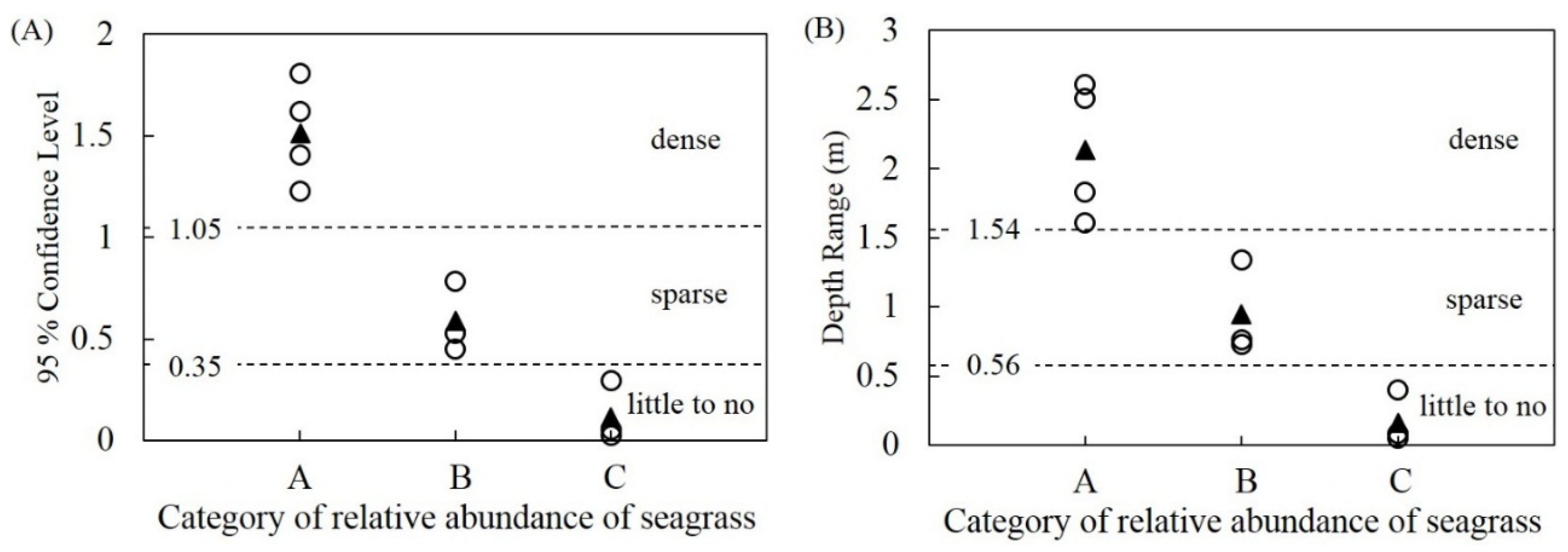
| A | 2, 3, 4, 5 | 1.51 | 0.22 | 2.14 | 0.43 | 5.74 |
| B | 1, 6, 8 | 0.59 | 0.14 | 0.95 | 0.28 | 5.77 |
| C | 7, 9, 10 | 0.11 | 0.12 | 0.16 | 0.16 | 6.02 |
3.3. 95% CL and Depth Range and Relative Abundance of Seagrass

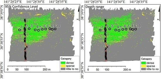
3.4. Distribution of Seagrass Meadows

| (A) 95% Confidence Level | Reference Data | User Accuracy | |||
| Dense | Sparse | No | |||
| Classified | Dense | 6 | 1 | 0 | 0.86 |
| Sparse | 1 | 1 | 0 | 0.50 | |
| Little to No | 4 | 0 | 17 | 0.81 | |
| Producer accuracy | 0.55 | 0.50 | 1.00 | Overall accuracy 0.80 | |
| (B) Depth Range | Reference Data | User Accuracy | |||
| Dense | Sparse | No | |||
| Classified | Dense | 8 | 1 | 1 | 0.80 |
| Sparse | 1 | 1 | 0 | 0.50 | |
| Little to No | 2 | 0 | 16 | 0.89 | |
| Producer accuracy | 0.73 | 0.50 | 0.94 | Overall accuracy 0.83 | |
4. Discussion
5. Conclusions
Acknowledgments
Author Contributions
Conflicts of Interest
References
- Boudouresque, C.F. Les Herbiers à Posidonia oceanica. In Préservation et Conservation des Herbiers à Posidonia Oceanica; Boudouresque, C.-F., Bernard, G., Bonhomme, P., Charbonnel, E., Diviacco, G., Meinesz, A., Pergent, G., Pergent-Martini, C., Ruitton, S., Tunesi, L.L., Eds.; Ramoge Publication: Monaco, 2006; pp. 10–24. [Google Scholar]
- Díaz-Almela, E.; Duarte, C.M. Management of Natura 2000 habitats. 1120* Posidonia beds (Posidonion oceanica); European Commission: Brussels, Belgium, 2008. [Google Scholar]
- Buchet, V. Impact Assessment of Invasive Flora Species in Posidonia Oceanica Meadows on Fish Assemblage: an Influence on Local Fisheries?: The Case Study of Lipsi Island, Greece. Master’s Thesis, University of Akureyri, Akureyri, Island, 31 March 2015. [Google Scholar]
- Duarte, C.M. The future of seagrass meadows. Environ. Conserv. 2002, 29, 192–206. [Google Scholar]
- Orth, R. J.; Carruthers, T.J.B.; Dennison, W.C.; Duarte, C.M.; Fourqurean, J.W.; Heck, K.L., Jr.; Randall, A.H.; Kendrick, G.A.; Kenworthy, W.J.; Olyarnik, S.; et al. A global crisis for seagrass ecosystems. Bioscience 2006, 56, 978–996. [Google Scholar] [CrossRef]
- Jackson, E.L.; Rowden, A.A.; Attrill, M.J.; Bossey, S.; Jones, M. The importance of seagrass beds as a habitat for fishery species. Oceanogr. Mar. Biol. 2001, 39, 269–304. [Google Scholar]
- Bertelli, C.M.; Unsworsth, R.K.F. Protecting the hand that feeds us: Seagrass (Zostera marina) serves as commercial juvenile fish habitat. Mar. Pollut. Bull. 2014, 83, 425–429. [Google Scholar] [CrossRef] [PubMed]
- Short, F.T.; Beth, P.; Livingstone, S.R.; Carpenter, K.E.; Salomão, B.; Bujang, J.S.; Calumpong, H.P.; Carruthers, T.J.B.; Coles, R.G.; Dennison, W.C.; et al. Extinction risk assessment of the world‘s seagrass species. Biol. Conserv. 2011, 144, 1961–1971. [Google Scholar] [CrossRef] [Green Version]
- Ward, L.G.; Kemp, W.M.; Boyton, W.R. The influence of waves and seagrass communities on suspended particulates in an estuarine embayment. Mar. Geol. 1984, 59, 85–103. [Google Scholar] [CrossRef]
- Jeudy de Grissac, A.; Boudouresque, C.-F. Rôle des herbiers de Phanérogames marines dans les mouvements des sédiments côtiers: Les herbiers à Posidonia oceanica. In Acte du Colloque Pluridisciplinaire Franco-Japonais d'Océanographie Fiscicule 1; Ceccaldi, H.J., Champalbert, G., Eds.; Société Franco-japonaise d’Océanographie, Marseille: Marseille, France, 1985; pp. 143–151. [Google Scholar]
- Komatsu, T. Influence of a Zostera bed on the spatial distribution of water flow over a broad geographical area. In Proceedings of an International Workshop Conference on Seagrass Biology, Nedlands, Australia, 25–29 January 1996; pp. 111–116.
- Komatsu, T.; Yamano, H. Influence of seagrass vegetation on bottom topography and sediment distribution on a small spatial scale in the Dravuni Island Lagoon, Fiji. Biol. Mar. Mediterr. 2000, 7, 243–246. [Google Scholar]
- Cullen-Unsworth, L.C.; Mtwana Nordlund, L.; Paddock, J.; Baker, S.; McKenzie, L.J.; Unsworth, R.K.F. Seagrass meadows globally as a coupled social-ecological system: Implications for human well-being. Mar. Pollut. Bull. 2014, 83, 387–397. [Google Scholar] [CrossRef] [PubMed]
- Costanza, R.D.; Arge, D.; de Groot, R.; Farber, S.; Grasso, M.; Hannon, B.; Limburg, K.; Naeem, S.; O‘Neill, R.V.; Paruelo, J.; et al. The value of the world’s ecosystem services and natural capital. Nature 1997, 387, 253–260. [Google Scholar] [CrossRef]
- Vassallo, P.; Paoli, C.; Rovere, A.; Montefalcone, M.; Morri, C.; Bianchi, C.N. The value of the seagrass Posidonia oceanica: A natural capital assessment. Mar. Pollut. Bull. 2013, 75, 157–167. [Google Scholar] [CrossRef] [PubMed]
- Meyer, W.B.; Turner, B.L. Human population growth and global land-use/cover change. Ann. Rev. Ecol. Syst. 1992, 23, 39–61. [Google Scholar] [CrossRef]
- World Bank. World Development Report 2003: Sustainable Development in a Dynamic World—Transforming Institutions, Growth, and Quality of Life; World Bank: New York, NY, USA, 2003. [Google Scholar]
- Tunesi, L.; Boudouresque, C.-F. Les Causes de la Régression Des Herbiers à Posidonia oceanica. In Préservation et Conservation Des Herbiers à Posidonia Oceanica; Boudouresque, C.-F., Bernard, G., Bonhomme, P., Charbonnel, E., Diviacco, G., Meinesz, A., Pergent, G., Pergent-Martini, C., Ruitton, S., Tunesi, L., Eds.; Ramoge Publication: Monaco, 2006; pp. 32–47. [Google Scholar]
- Komatsu, T. Long-term changes in the Zostera bed area in the Seto Inland Sea (Japan), especially along the coast of the Okayama Prefecture. Oceanol. Acta 1997, 20, 209–216. [Google Scholar]
- Komatsu, T.; Sagawa, T.; Sawayama, S.; Tanoue, H.; Mohri, A.; Sakanishi, Y. Mapping Is a Key for Sustainable Development of Coastal Waters: Examples of Seagrass Beds and Aquaculture Facilities in Japan with Use of ALOS Images. In Sustainable Development; Ghenai, C., Ed.; Tech Publishing Co.: Rijeka, Croatia, 2012; pp. 145–160. [Google Scholar]
- Kirkman, H. Seagrass distribution and mapping. Seagrass research methods. Monogr. Oceanogr. Methodol. 1990, 9, 19–25. [Google Scholar]
- Komatsu, T.; Mikami, A.; Sultana, S.; Ishida, K.; Hiraishi, T.; Tatsukawa, K. Hydro-acoustic methods as a practical tool for cartography of seagrass beds. Otsuchi Mar. Sci. 2003, 28, 72–79. [Google Scholar]
- Hashim, M.; Yahya, N.N.; Ahmad, S.; Komatsu, T.; Misbari, S.; Reba, M.N. Determination of seagrass biomass at Merambong Shoal in Straits of Johor using satellite remote sensing technique. Malay. Nat. J. 2014, 66, 20–37. [Google Scholar]
- Sagawa, T.; Boisnier, E.; Komatsu, T.; Mustapha, K.B.; Hattour, A.; Kosaka, N.; Miyazaki, S. Using bottom surface reflectance to map coastal marine areas: A new application method for Lyzenga’s model. Int. J. Remote Sens. 2010, 31, 3051–3064. [Google Scholar] [CrossRef]
- Phinn, S.; Roelfsema, C.; Dekker, A.; Brando, V.; Anstee, J. Mapping seagrass species, cover and biomass in shallow waters: An assessment of satellite multispectral and airborne hyper-spectral imaging systems in Moreton Bay (Australia). Remote Sens. Environ. 2008, 112, 3413–3425. [Google Scholar] [CrossRef]
- Kotchenova, S.Y.; Song, X.; Shabanov, N.V.; Potter, C.S.; Knyazikhin, Y.; Myeni, R.B. Lidar remote sensing for modeling gross primary production of deciduous forests. Remote Sens. Environ. 2004, 92, 158–172. [Google Scholar] [CrossRef]
- Maltamo, M.; Eerikainen, K.; Pitkainen, J.; Hyppa, J.; Vemas, M. Estimation of timber volume and stem density based on scanner laser altimetry and expected size distribution functions. Remote Sens. Environ. 2004, 90, 319–330. [Google Scholar] [CrossRef]
- Hamilton, L.J. Real-time echosounder based acoustic seabed segmentation with two first echo parameters. Methods Oceanogr. 2014, 11, 13–28. [Google Scholar] [CrossRef]
- Komatsu, T.; Tatsukawa, K. Mapping of Zostera marina L. beds in Ajino Bay, Seto Inland Sea, Japan, by using echosounder and global positioning systems. J. Rech. Oceanogr. 1998, 23, 39–46. [Google Scholar]
- Sabol, B.M.; Melton, R.E.; Chamberlain, R.; Doering, P.; Haunert, K. Evaluation of a digital echo sounder system for detection of submersed aquatic vegetation. Estuaries 2002, 25, 133–141. [Google Scholar] [CrossRef]
- Newton, R.S.; Stefanon, A. Application of side scan sonar in marine biology. Mar. Biol. 1975, 31, 287–291. [Google Scholar] [CrossRef]
- Meinesz, A.; Cuvelier, M.; Laurent, R. Méthode récentes de cartographie et de surveillance des herviers de Phanérogames marines. Vie Milieu 1981, 31, 27–34. [Google Scholar]
- Lefèvre, J.R.; Meinesz, A.; Gloux, B. Premières Données sur la Comparaison de Trois Méthôdes de Cartographie des Biocénoses Marines; Commission Internationale pour L’Exploration Scientifique de la Mer Méditerranée (CIESM): Monaco, 1984. [Google Scholar]
- Gloux, B. Méthode Acoustiques et Informatiques Appliquées à la Cartographie Rapide et Détaillée Des Herbiers. In International Workshop on Posidonia oceanica Beds; Boudouresque, C.-F., Jeudy de Grissac, A., Olivier, J., Eds.; GIS Posidonie Press: Marseille, France, 1984; pp. 45–48. [Google Scholar]
- Ramos, M.A.; Ramos-Espla, A. Utilization of acoustic methods in the cartography of the Posidonia oceanica bed in the bay of Alicante (SE, Spain). Pos. Newslett. 1989, 2, 17–19. [Google Scholar]
- Pasqualini, V.; Pergent-Martini, C.; Clabaut, P.; Pergent, G. Mapping of Posidonia oceanica using aerial photographs and side scan sonar: Application off Island of Corsica (France). Estuar. Coast. Shelf Sci. 1998, 47, 359–367. [Google Scholar] [CrossRef]
- Komatsu, T.; Igarashi, C.; Tatsukawa, K.; Matsuoka, Y.; Harada, S.; Sultana, S. Use of multi-beam sonar to map seagrass beds in Otsuchi Bay, on the Sanriku Coast of Japan. Aquat. Living Resour. 2003, 16, 223–230. [Google Scholar] [CrossRef]
- Komatsu, T.; Ben Mustapha, K.; Shibata, K.; Hantani, K.; Ohmura, T.; Sammari, C.; Igarashi, C.; El Abed, A. Mapping Posidonia Meadows on Messioua Bank off Zarzis, Tunisia, Using Multi-Beam Sonar and GIS. In GIS/Spatial Analyses in Fisheries and Aquatic Sciences; Nishida, T., Kaiola, P.J., Hollingworth, C.E., Eds.; Fishery-Aquatic GIS Research Group: Saitama, Japan, 2004; pp. 83–100. [Google Scholar]
- Parnum, I.M.; Gavrilov, A.N. High-frequency multibeam echo-sounder measurements of seafloor backscatter in shallow water: Part 1–Data acquisition and processing. Underw. Technol. 2011, 30, 3–12. [Google Scholar] [CrossRef]
- Tecchiato, S.; Collins, L.; Parnum, I.; Stevens, A. The influence of geomorphology and sedimentary processes on benthic habitat distribution and littoral sediment dynamics: Geraldton, Western Australia. Mar. Geol. 2015, 359, 148–162. [Google Scholar] [CrossRef]
- De Falco, G.; Tonielli, R.; di Martino, G.; Innangi, S.; Simeone, S.; Michael Parnum, I. Relationships between multibeam backscatter, sediment grain size and Posidonia oceanica seagrass distribution. Cont. Shelf Res. 2010, 30, 1941–1950. [Google Scholar] [CrossRef]
- Parnum, I.M. Benthic Habitat Mapping Using Multibeam Sonar System. PhD Thesis, Department of Imaging and Applied Physics, Curtin University of Technology, Perth, Australia, 2007; p. 213. [Google Scholar]
- Lyons, A.P.; Abraham, D.A. Statistical characterization of high-frequency shallow-water seafloor backscatter. J. Acoust. Soc. Am. 1999, 106, 1307–1315. [Google Scholar] [CrossRef]
- Riegl, B.; Moyer, R.P.; Morris, L.; Virnstein, R.; Dodge, R.E. Determination of the distribution of shallow-water seagrass and drift algae communities with acoustic searfloor discrimination. Rev. Biol. Trop. 2005, 53, 165–174. [Google Scholar] [PubMed]
- Wilson, P.S.; Dunton, K.H. Laboratory investigation of the acoustic response of seagrass tissue in the frequency band 0.5–2.5 kHz. J. Acoust. Soc. Am. 2009, 125, 1951–1959. [Google Scholar] [CrossRef] [PubMed]
- Anderson, J.T.; van Holliday, D.; Kloser, R.; Reid, D.G.; Simard, Y. Acoustic seabed classification: Current practice and future directions. ICES J. Mar. Sci. J. Cons. 2008, 65, 1004–1011. [Google Scholar] [CrossRef]
- Di Maida, G.; Tomasello, A.; Luzzu, F.; Scannavino, A.; Pirrotta, M.; Orestano, C.; Calvo, S. Discriminating between Posidonia oceanica meadows and sand substratum using multibeam sonar. ICES J. Mar. Sci. J. Cons. 2011, 68, 12–19. [Google Scholar] [CrossRef]
- Lurton, X. An Introduction to Underwater Acoustics: Principles and Applications; Springer: Berlin, Germany, 2002; p. 347. [Google Scholar]
- Komatsu, T.; Ohtaki, T.; Sakamoto, S.; Sawayama, S.; Hamana, Y.; Shibata, M.; Shibata, K.; Sasa, S. Impact of the 2011 Tsunami on Seagrass and Seaweed Beds in Otsuchi Bay, Sanriku Coast, Japan. In Marine Productivity: Perturbations and Resilience of Socio-Ecosystems; Ceccaldi, H.J., Hénocque, Y., Koike, Y., Komatsu, T., Stora, G., Tusseau-Vuillemin, M.-H., Eds.; Springer International Publishing AG: Cham, Switzerland, 2015; pp. 43–53. [Google Scholar]
- Sakamoto, S.X.; Sasa, S.; Sawayama, S.; Tsujimoto, R.; Terauchi, G.; Yagi, H.; Komatsu, T. Impact of huge tsunami in March 2011 on seaweed bed distributions in Shizugawa Bay, Sanriku Coast, revealed by remote sensing. Proc. SPIE 2012. [Google Scholar] [CrossRef]
- Sasa, S.; Sawayama, S.; Sakamoto, S.; Tsujimoto, R.; Terauchi, G.; Yagi, H.; Komatsu, T. Did huge tsunami on 11 March 2011 impact seagrass bed distributions in Shizugawa Bay, Sanriku Coast, Japan? Proc. SPIE 2012. [Google Scholar] [CrossRef]
- Applanix Corp. POS MV V5 Installation and Operation Guide. Document # PUBS-MAN-004291, Revision: 11, Date: 8-December-2015. Available online: www.applanix.com/products/marine/pos-mv/423-operations-manual-v5-.html (accessed on 22 January 2016).
- Short, F.T.; McKenzie, L.J.; Coles, R.G.; Vidler, K.P. Seagrassnet Manual for Scientific Monitoring of Seagrass Habitat; Queensland Department of Primary Industry, Queensland Fisheries Service: Cairns, Australia, 2002; p. 56.
- Almar, H. How to Total Propagated Uncertainty. from QPS. Available online: https://confluence.qps.nl/s/-wQfAg (accessed on 21 August 2015).
- Almar, H. Tips and Tricks. Retrieved 16 September 2015, from QPS. Available online: https://confluence.qps.nl/x/3QwfAg (accessed on 16 September 2015).
- IHO (International Hydrographic Organization). IHO Standards for Hydrographic Surveys; IHO: Monaco, 2008; p. 17. [Google Scholar]
- Innangi, S.; Barra, M.; di Martino, G.; Parnum, I.M.; Tonielli, R.; Mazzola, S. Reson SeaBat 8125 backscatter data as a tool for seabed characterization (Central Mediterranean, Southern Italy): Results from different processing approaches. Appl. Acoust. 2015, 87, 109–122. [Google Scholar] [CrossRef]
© 2016 by the authors; licensee MDPI, Basel, Switzerland. This article is an open access article distributed under the terms and conditions of the Creative Commons by Attribution (CC-BY) license (http://creativecommons.org/licenses/by/4.0/).
Share and Cite
Hamana, M.; Komatsu, T. Real-Time Classification of Seagrass Meadows on Flat Bottom with Bathymetric Data Measured by a Narrow Multibeam Sonar System. Remote Sens. 2016, 8, 96. https://0-doi-org.brum.beds.ac.uk/10.3390/rs8020096
Hamana M, Komatsu T. Real-Time Classification of Seagrass Meadows on Flat Bottom with Bathymetric Data Measured by a Narrow Multibeam Sonar System. Remote Sensing. 2016; 8(2):96. https://0-doi-org.brum.beds.ac.uk/10.3390/rs8020096
Chicago/Turabian StyleHamana, Masahiro, and Teruhisa Komatsu. 2016. "Real-Time Classification of Seagrass Meadows on Flat Bottom with Bathymetric Data Measured by a Narrow Multibeam Sonar System" Remote Sensing 8, no. 2: 96. https://0-doi-org.brum.beds.ac.uk/10.3390/rs8020096