Comparing Near Coincident Space Borne C and X Band Fully Polarimetric SAR Data for Arctic Sea Ice Classification

Abstract

This work compares the polarimetric backscatter behavior of sea ice in spaceborne X-band and C-band Synthetic Aperture Radar (SAR) imagery. Two spatially and temporally coincident pairs of fully polarimetric acquisitions from the TerraSAR-X/TanDEM-X and RADARSAT-2 satellites are investigated. Proposed supervised classification algorithm consists of two steps: The first step comprises a feature extraction, the results of which are ingested into a neural network classifier in the second step. Based on the common coherency and covariance matrix, we extract a number of features and analyze the relevance and redundancy by means of mutual information for the purpose of sea ice classification. Coherency matrix based features which require an eigendecomposition are found to be either of low relevance or redundant to other covariance matrix based features, which makes coherency matrix based features dispensable for the purpose of sea ice classification. Among the most useful features for classification are matrix invariant based features (Geometric Intensity, Scattering Diversity, Surface Scattering Fraction). This analysis reveals analogous results for all four acquisitions, in both X-band and C-band frequencies. The subsequent classification produces similarly promising results for all four acquisitions. In particular, the overlapping image portions exhibit a reasonable congruence of detected ice types.

1. Introduction

Over more than three decades, researchers have been utilizing Synthetic Aperture Radar (SAR) to monitor ice covered maritime regions. The major advantages of satellite borne SAR over optical imaging is its applicability, irrespective of clouds and daylight. Satellite borne SAR is capable of covering almost any region on earth with short recurrence periods (at least daily), even during rough weather conditions. This last point is particularly helpful in the surveillance of sea ice, which is mostly encountered in remote latitudes. Spaceborne SAR platforms such as RADARSAT-1 and RADARSAT-2 (RS-2), ERS or ENVISAT in C-band, ALOS PALSAR in L-band, and Cosmo-Skymed or TerraSAR-X/TanDEM-X (TS-X) in X-band have demonstrated the added benefit SAR sensors can give in the investigation of sea ice in Arctic and Antarctic regions ([1,2,3,4]). A single acquisition of a SAR sensor can cover a stretch on the ground of up to a few hundred kilometers in azimuth and range: 100 km × 150 km (range, azimuth) in the case of ScanSAR TS-X, and 500 km × 500 km in case of ScanSAR Wide RS-2. Such wide area coverage is particularly useful during field campaigns in the marginal ice zone (Office of Naval Research Marginal Ice Zone campaign, 2015). When detailed information is of greater interest than large coverage (as is for this work), other SAR modes with several polarimetric image channels and high resolution (at the price of large ground coverage) can meet this demand as well. Some special topics in sea ice research are ice drift ([5,6]), ice concentration ([7]), iceberg detection ([8,9]), and sea state and wave propagation into sea ice ([10,11]). Most research published so far on SAR based sea ice classification concentrates on single polarimetric data (e.g., [12,13,14,15,16,17,18,19,20,21]). Mentioned work on sea ice classification naturally concentrates on classical image analysis in one channel: By inspection of image intensity or higher order statistics of local image intensities, one strives to characterize each pixel or neighborhood, possibly after segmenting the image. Popular techniques are texture analysis (second order statistics of neighborhoods) via Gray Level Co-occurrence Matrices (GLCM), (cf. [12,13,14,15,17,18,22,23]), autocorrelation methods ([24]), wavelet based features ([10,25,26]), Gabor wavelet techniques ([12]), and Markov random fields (MRF) ([16]). Efforts have been undertaken to improve the classification quality based on single pol SAR data by data fusion with scatterometer data ([27]) from AMSR-2 or by model data based on previously known ice drift ([5]), where model output is fused with SAR classification by segmentation/texture analysis. Despite the usefulness and success of such tools, certain major issues in sea ice classification still defy a solution in any of the mentioned approaches. Most notably, different ice types exhibit high variation in gray scale and texture depending on incidence angle [28], weather conditions, geography and season (see [29] and references therein).

Polarimetric data (i.e., complex linear dual-polarimetric of full-polarimetric images) may be able to overcome some of the mentioned obstacles, due to the higher information content of multiple channels in different polarizations compared to single polarimetric data. The earliest works of SAR based sea ice research already took advantage of polarimetric SAR imagery. Namely the works of [22,30] describe a neural network based, iterative classification on airborne C-, L-, and P-band full-polarimetric images, using intensities and phase differences to discriminate ice into 3 classes. Similarly, [31] used such airborne C-, L-, and P-band full-polarimetric SAR data with channel intensity ratios and phase differences for a decision tree-based classification. Given that longer wavelengths have greater penetration depths into ice, [32] was able to relate ice thickness to airborne L-band SAR backscatter, employing phase differences and intensity ratios. The twin publication of [33,34] discussed the theoretical aspects of SAR backscatter in ice and related this discussion to ice classification of (airborne) C- and L-band polarimetric SAR data. A review of these earlier SAR-based sea ice classification approaches on polarimetric data can be found in [35]. The most powerful recurring feature in all these works prove to be intensity ratios, which are even used in dual polarimetric scatterometer data for open water—sea ice discrimination, see [36]. With the advent of new spaceborne polarimetric SAR sensors, investigation in the field of sea ice classification was continued. The work of [29,37] which compare JERS-1 L-band polarimetric data with C-band ERS data shows the suitability and differences of SAR for identification of sea ice structures. The features used for discrimination (in a decision tree) used in [29,37] comprise intensities, phase differences and intensity ratios. In the same fashion, relying on intensity ratios with stunning success, [38] classify the sea ice types in a number of Envisat ASAR images.

Despite all the success which mentioned research on sea ice has produced, more elaborate analytical ideas, most notably the H/A/α analysis by [39], allows the user to gain deeper insight into the backscatter behavior of sea ice types. This path of enriching the feature set by features derived from scattering matrix invariants, we strive to follow in this publication. The most popular analysis is the Eigen-decomposition based H/A/α approach ([39,40,41]), which derives polarimetric features and electromagnetic properties of the scattering surface from the Pauli scattering matrix (commonly called coherency matrix). Whereas [40] concentrates on L-band data, we are concerned with the comparison of C-band and X-band data. The underlying datasets were acquired with high temporal and spatial correlation (see

Table 1. Description of TerraSAR-X (Quadpol) and RADARSAT-2 (Quadpol) images used in this study. * DRA—Dual Receive Antenna (Experimental Mode), SM—StripMap, FQ—FineQuad, Asc.—Ascending pass.

Date, Time (UTC)	Sensor	Inc.	Pass	Imaging	Slant Rg./	Footpr. Az.	Number
		Ang.	Mode	Mode	Az. Res. (m)	Rg. per Frame	of Frames
2015/04/19, 14:51	TS-X *	39${}^{°}$–40${}^{°}$	Asc.	SM	1.2 m/6 m	55 km/18.5 km	2
2015/04/19, 13:19	RS-2	21${}^{°}$–23${}^{°}$	Asc.	FQ	5.2 m/7.6 m	35 km/27 km	3
2015/04/23, 13:43	TS-X *	27${}^{°}$–29${}^{°}$	Asc.	SM	1.2 m/6 m	55 km/18.5 km	3
2015/04/23, 14:42	RS-2	36${}^{°}$–38${}^{°}$	Asc.	FQ	5.2 m/7.6 m	35 km/27 km	2

, Figure 1). One common method to classify a generic SAR image (not only for sea ice) based on polarimetric features is the unsupervised Wishart classification ([41,42]), a more recent method ([43]) uses Riemannian manifold classification, that does not rely on particular parametric assumptions on the distributions. In addition to quad polarimetric SAR, compact polarimetry has been found to offer a good compromise between the number of polarization channels and coverage (see [44]). A recent study by Dabboor et al. ([45]) presents simulations of compact polarimetric response from sea ice for the purpose of sea ice classification with promising results. In the works of Moen et al. ([46,47]), polarimetric SAR imagery in C-band data was investigated using a segmentation prior to an automated, statistical-distance based labeling of the segments for sea ice classification. The automatic segmentation is juxtaposed with manual segmentations, yielding improved quality over manual classification. Above mentioned works mostly focused on relating physical scattering behavior with particular polarimetric features. The analyses of [46,47] qualitatively examined the plausibility of the different outcomes of manual and automatic classification approaches. Our work has a different focus by contributing first a comprehensive quantification of the information content of Eigen-decomposition based polarimetric features (H/A/α) and other polarimetric features derived from the scattering matrix (see [48]) in X-band and in C-band individually. Afterwards, the two results are compared in the overlapping portions of the C-band and X-band images.

The underlying datasets are two pairs of near-coincident (temporally and spatially) acquisitions of quad-polarimetric images in X-band (TerraSAR-X) and in C-band (RADARSAT-2). Until now, no such direct comparison on near-coincident, quad-polarimetric spaceborne SAR data acquired over the Arctic has been conducted. This temporal and spatial correlation of C and X-band quad polarimetric data allows us to make statements on the backscatter behavior which can be regarded as rather unaffected by any uncertainty related to space and time variation impact. In our research, we are motivated by establishing an automated sea ice classification algorithm for navigational ice charting. This also justifies a deeper analysis of the information content of the features before we perform classification. Directly linking clusters in the feature space to certain ice types (or physical properties of ice types) is a rather cumbersome endeavor in high dimensions. Therefore, we train an artificial neural network (ANN) classifier, which reflects such nonlinear relationships between features and ice type. Such an ANN has been utilized in the field of sea ice classification before (see [17,18,21]). For details about the classifier, in particular its implementation, the reader is referred to [21,49].

Above discussions guide the structure of our publication: We will first introduce our datasets and the polarimetric features. Followed by an information theoretic analysis of the polarimetric features on all samples of training datasets. The key statistical technique will rely on the concept of mutual information (cf. [50]). By this analysis, we can quantify the redundancy and relevance of polarimetric features for our purposes of identifying different ice types. In the third section, we present the output of our subsequent pixel-based neural network classification and cross-compare the results for the simultaneous, overlapping image portions. For the classification, we take advantage of an open source neural network library (FANN, see [49]), wherefore the reader is referred to standard literature on the theory and application of neural networks or to consult [18] for successful use of neural network sea ice classification on SAR images.

2. Experimental Dataset

In this work we want to explore sea ice classification on full-polarimetric SAR data in high resolution, where the latter naturally comes at the price of a smaller footprint for both satellites TS-X and RS-2. A list of the SAR acquisitions with the respective technical parameters can be found in Table 1. We remark that each acquisition consists of two or three frames (Frame refers to standard acquisition coverage, see Figure 1 and Table 1). In case of the RS-2 acquisitions, the mode is fine quadpol (FineQuad, FQ). In case of TS-X, the images are StripMap images.

The images were located between the latitudes 82.4 and 83.4 North and longitudes 11 and 23 East, in the Arctic Ocean. Precise coordinates will be displayed in the result Section 5.

These X-band quad pol datasets were acquired using Dual Receive Antenna (DRA) configuration mode, which is not yet commercially available. The X- band fully polarimetric data which were acquired over the study area are quite unique over ice infested regions (during science phase, [51]). For each day of data acquisition, one sensor was capturing in near range and the other in far range, with reversed roles of TS-X and RS-2 for the two dates. This enables us to assess the ice classification quality in far and near range for both sensors (see Table 1 for incidence angle ranges). As training dataset we chose small image patches from all four acquisitions from each of the dominant ice types. The variation in backscatter behavior of the four acquisitions differ due to different sensors or incidence angle range, such that it is not advisable to apply a classifier generated on training data from one acquisition to any other acquisition (cf. [46,47]). To add more plausibility to the choice of dominant ice types, the reader may consider the coarse resolution ice thickness for the area on 15 April 2015 according to L3C SMOS data (icdc.zmaw.de/daten/cryosphere/l3c-smos-sit.html), which is corroborated by ice concentration for the area reported by the Norwegian Ice Services. According to NASA MODIS data from 15 April 2015 to 23 April 2015 (OB.DAAC, see Section of Acknowledgments), the sea surface temperature in the region of acquisitions stayed below $-8^{°}$ Celsius (apart from open water portions), which indicates that freezing conditions persisted from 15 April 2015 to 23 April 2015. Based on these ancillary data, training data rectangles in the image were determined by visual interpretation of feature images in conjunction with archive data of usual ice situation for the location and time of the year. Ice concentration charts of the Norwegian ice service reported a local average sea ice concentration of 100%. According to NASA MODIS data on 19 April 2015 and 23 April 2015 (OB.DAAC, see Section of Acknowledgments), the sea surface temperature in the region of acquisitions is below $-{10}^{°}$ Celsius (apart from open water portions), wherefore we conclude that thaw onset can be has not occurred for our dataset. The regime of dominant ice classes found were Open Water/nilas (OW), Young Ice (YI), Smooth First Year (SFYI) ice and a mixture of rough first-year and multi-year ice (RFYMYI). Since open water and nilas are rather difficult to discriminate in many features, and since we work towards an operational ice chart for navigation, we find it appropriate to merge these two ice types. To sketch the reasonings for picking characteristic ice types in the images, we consider the feature images of the TS-X acquisition in Figure 2: open water portions are known to be detectable by the co-pol power ratio ([29]). A higher value in the geometric intensity μ indicates older ice (RFYMYI, yellow-red textured ice portions) that has undergone more deformations than first year ice (SFYI) with lower geometric intensity values (blue areas in geometric intensity, Figure 2). Broken up leads, where the co-pol power ratio indicates ice coverage rather than open water are likely to be refrozen open water and are thus categorized as young ice (see greenish portions of leads in 2, eigenvalue 2).

3. Polarimetric Features

Research on C-band and L-band and X-band SAR backscatter behavior was conducted before (e.g., [29,46,47,52,53]). In particular due to similar frequencies of X-band and C-band, we expected to find analogous behavior of TS-X and RS-2 for similar incidence angles. Preceding our discussion of the expected behavior in C-band and X-band, we propose our quad-polarimetric and dual-polarimetric definition for the features. Even though for the latter category of features, we discarded some information, we computed the dual-polarimetric features in order to sound out the added value of full polarimetry over dual polarimetry in sea ice classification. Such insight with respect to quality is in particular important for TS-X based operational purposes, since quad-pol imagery is commercially not available for this sensor. The dual polarimetric version of features is denoted with a $\left(d\right)$ superscript, the $\left(q\right)$ superscript is the quad-polarimetric version of the feature. We note that every feature is derived for each acquisition and sensor.

Delivered data were calibrated according to the respective specification of the sensor by the formula. In case of TS-X, this was done by

$$S_{XY}\left(x\right)=\sqrt{k·sin\left(\beta \right(x\left)\right)}·D{N}_{XY}\left(x\right)$$

(1)

where $\beta \left(x\right)$ denotes the incidence angle at pixel location x, k denotes the calibration factor, and $D{N}_{XY}\left(x\right)$ the delivered complex pixel value of the $XY$ polarization (in slant range), $X,Y\in \{H,V\}$. The complex backscatter return is denoted by $S_{XY}$. For RS-2, the calibration was carried out through

$$S_{XY}=DN\left(x\right)·Gains\left(x\right)$$

(2)

where $Gains\left(x\right)$ denotes a delivered calibration matrix, accounting for incidence angle and other technical constants. ${\sigma }_{XY}$ denotes the absolute of $S_{XY}$ and ${\varphi }_{XY}$ denotes the phase angle of $S_{XY}$, with $X,Y\in \{H,V\}$, i.e.,

$$S_{XY}={\sigma }_{XY}exp\left(i{\varphi }_{XY}\right)$$

(3)

The brackets $\langle ·\rangle$ symbolize the local averaging process during polarimetric feature extraction. (The spatial averaging window size was chosen to be 11 pixels for our sample dataset throughout this publication.) The scattering vector is commonly analyzed with respect to the lexicographic basis and the Pauli basis. The resulting scattering matrices (averaged covariances) are the well-known coherency matrix $T_3$ and covariance matrix $S_3$:

$$T_3=\frac{1}{\sqrt{2}}\left(\begin{array}{ccc}\langle {|S_{HH}+S_{VV}|}^2\rangle & \langle (S_{HH}+S_{VV}){(S_{HH}-S_{VV})}^{*}\rangle & \langle (S_{HH}+S_{VV}){\left(2S_{HV}\right)}^{*}\rangle \\ \langle {(S_{HH}+S_{VV})}^{*}(S_{HH}-S_{VV})\rangle & \langle {|S_{HH}-S_{VV}|}^2\rangle & \langle (S_{HH}-S_{VV}){\left(2S_{HV}\right)}^{*}\rangle \\ \langle {(S_{HH}+S_{VV})}^{*}\left(2S_{HV}\right)\rangle & \langle {(S_{HH}-S_{VV})}^{*}\left(2S_{HV}\right)\rangle & \langle {\left|2\left(S_{HV}\right)\right|}^2\rangle \end{array}\right)$$

(4)

$$S_3=\left(\begin{array}{ccc}\langle {\left|S_{HH}\right|}^2\rangle & \langle \left(S_{HH}\right){\left(S_{VV}\right)}^{*}\rangle & \langle \left(S_{HH}\right){\left(S_{HV}\right)}^{*}\rangle \\ \langle {\left(S_{HH}\right)}^{*}\left(S_{VV}\right)\rangle & \langle {\left|S_{VV}\right|}^2\rangle & \langle \left(S_{VV}\right){\left(S_{HV}\right)}^{*}\rangle \\ \langle {\left(S_{HH}\right)}^{*}\left(S_{HV}\right)\rangle & \langle {\left(S_{VV}\right)}^{*}\left(S_{HV}\right)\rangle & \langle {\left|S_{HV}\right|}^2\rangle \end{array}\right)$$

(5)

The dual-polarimetric versions were then defined as

$$T_2=\left(\begin{array}{cc}{T}_3(1,1)& T_3(1,2)\\ T_3(2,1)& T_3(2,2)\end{array}\right)$$

(6)

and

$$S_2=\left(\begin{array}{cc}{S}_3(1,1)& S_3(1,2)\\ S_3(2,1)& S_3(2,2)\end{array}\right)$$

(7)

The particular features were inspired by the ones outlined in [39,48,54].

The (quad-polarimetric) eigenvalues ${\lambda }_1^{\left(q\right)}$,${\lambda }_2^{\left(q\right)}$, and ${\lambda }_3^{\left(q\right)}$ of $T_3$ and the (dual-polarimetric) eigenvalues ${\lambda }_1^{\left(d\right)}$, and ${\lambda }_2^{\left(d\right)}$ of $T_2$ were used to compute $p_j^{\left(q\right)}={\lambda }_j^{\left(q\right)}/({\lambda }_1^{\left(q\right)}+{\lambda }_2^{\left(q\right)}+{\lambda }_3^{\left(q\right)})$ and $p_j^{\left(d\right)}={\lambda }_j^{\left(d\right)}/({\lambda }_1^{\left(d\right)}+{\lambda }_2^{\left(d\right)})$. This was the input for deriving entropy

$$H^{\left(q\right)}=-\left(p_1^{\left(q\right)}{log}_3\left(p_1^{\left(q\right)}\right)+p_2^{\left(q\right)}{log}_3\left(p_2^{\left(q\right)}\right)+p_3^{\left(q\right)}{log}_3\left(p_3^{\left(q\right)}\right)\right)$$

(8)

and

$$H^{\left(d\right)}=-\left(p_1^{\left(d\right)}{log}_2\left(p_1^{\left(d\right)}\right)+p_2^{\left(d\right)}{log}_2\left(p_2^{\left(d\right)}\right)\right)$$

(9)

and anisotropy

$$A^{\left(q\right)}=\frac{(p_2^{\left(q\right)}-p_3^{\left(q\right)})}{(p_2^{\left(q\right)}+p_3^{\left(q\right)})}$$

(10)

and

$$A^{\left(d\right)}=\frac{(p_1^{\left(d\right)}-p_2^{\left(d\right)})}{(p_1^{\left(d\right)}+p_2^{\left(d\right)})}$$

(11)

From the eigenvectors $v_1^{\left(q\right)},v_2^{\left(q\right)},v_3^{\left(q\right)}$ of $T_3$ one obtains

$${\alpha }_i^{\left(q\right)}=arccos(v_j^{\left(q\right)}\left(1\right)),j=1,2$$

(12)

For comparison we also computed from the $T_2$ matrix the ${\alpha }^{\left(d\right)}$ angles (defined analogously with eigenvectors $v_j^{\left(d\right)}$ of $T_2$ instead of $v_j^{\left(q\right)}$), simply for the sake of comparison of quad-polarimetric and dual-polarimetric data.The average α angle we defined by

$${\alpha }^{\left(q\right)}={\alpha }_1^{\left(q\right)}{p}_1^{\left(q\right)}+{\alpha }_2^{\left(q\right)}{p}_2^{\left(q\right)}+{\alpha }_3^{\left(q\right)}{p}_3^{\left(q\right)}$$

(13)

and analogously for the dual-polarimetric case

$${\alpha }^{\left(d\right)}={\alpha }^{\left(d\right)}{p}_1^{\left(d\right)}+{\alpha }_2^{\left(d\right)}{p}_2^{\left(d\right)}$$

(14)

whereas the classical $H^{\left(q\right)}/A^{\left(q\right)}/{\alpha }^{\left(q\right)}$ features (cf. [39]) in the fully polarimetric case have a well-established physical interpretation (e.g., about predominant scattering mechanisms), such interpretation cannot be expected to hold for our dual-polarimetric adaptions $H^{\left(d\right)}/A^{\left(d\right)}/{\alpha }^{\left(d\right)}$. Nonetheless, the dual-polarimetric Pauli based features bear statistical information (possibly without physical meaning) that can characterize different types of sea ice surfaces.

From $S_2$ and $S_3$ we derived a number of features, inspired by [54] and by [48]:

Copolarization power ratio:

$$\gamma =\frac{\langle {\left|S_{HH}\right|}^2\rangle }{\langle {\left|S_{VV}\right|}^2\rangle }$$

(15)

Copol phase difference:

$$\Delta \varphi ={\varphi }_{HH}-{\varphi }_{VV}$$

(16)

Real part of the copolarization cross product:

$$\rho =\left|\Re \langle S_{HH}{S}_{VV}^{*}\rangle \right|$$

(17)

Correlation:

$$\epsilon =\frac{\langle S_{HH}{S}_{VV}^{*}\rangle }{\sqrt{\langle {\left|S_{HH}\right|}^2\rangle \langle {\left|S_{VV}\right|}^2\rangle }}$$

(18)

Span of $T_2$ and $T_3$:

$$spa{n}^{\left(d\right)}=\mathrm{trace}\left(T_2\right)$$

(19)

and

$$spa{n}^{\left(q\right)}=\mathrm{trace}\left(T_3\right)$$

(20)

Scattering diversity (where ${\parallel ·\parallel }_F$ denotes the matrix Frobenius norm):

$$\delta =\frac{3}{2}\left(1-{\left(\frac{{\parallel T_3\parallel }_F}{spa{n}^{\left(q\right)}}\right)}^2\right)$$

(21)

Surface scattering fraction:

$$\tau =\frac{\langle {|S_{HH}+S_{VV}|}^2\rangle }{span}$$

(22)

Geometric Intensity μ:

$$\mu ={\left(det\left(T_3\right)\right)}^{(1/3)}$$

(23)

As a filtering of feature matrices, we employed a 5 by 5 pixel median filter to reduce noise effects. Both the C-band and the X-band co-pol power ratio have have been proven to be an excellent measure to distinguish open water and all other ice types, in particular older and thicker ice types ([29], [38], or [52]), given the incidence angle is not too low (according to [38] above 27${}^{°}$ for C-band) and low to moderate wind speeds (less than 14m/s in C-band according to [38]). In case of the younger ice types, the co-pol power ratio is not as powerful in discriminating such thin ice from open water. The C-band copolarized phase difference $\Delta \varphi$ was found to be useful for discriminating certain thinner ice types ([29,46,53]). For L-band, quad-polarimetric entropy $H^{\left(q\right)}$ is known to discriminate open water from ice types generally well and also thin ice from thick ice types due to the underlying different scattering mechanisms ([40]). (Quad-polarimetric) L-band anisotropy $A^{\left(q\right)}$ is known to be sensitive to surface roughness ([40]). In the dual-pol case, the classical physical meaning of anisotropy $A^{\left(d\right)}$ does not hold in general. $A^{\left(d\right)}$ is nearly equivalent to $H^{\left(d\right)}$ for purely mathematical reasons (see [55]).

4. Mutual Information, Relevance and Redundancy of Features

Since we want to study the suitability of polarimetric features for sea ice classification, we will first roughly discuss by visual impression the information content of some features. The limitations of such impression then lead us to rigorously analyze the information content of each feature and their redundancy with respect to sea ice classification.

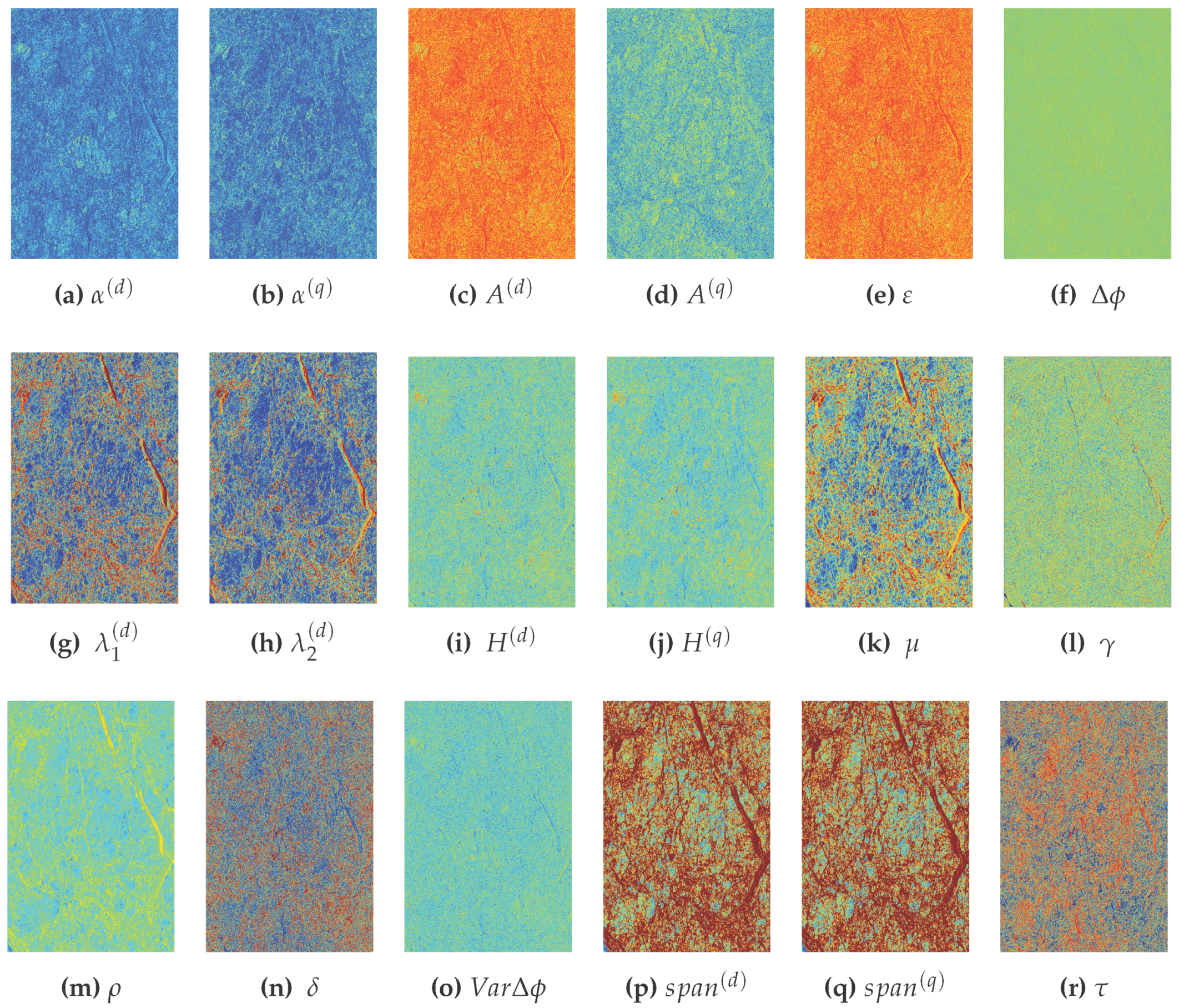
In order to obtain a first impression about the predictive quality of the different features, i.e., their capacity to predict the ice class, we display all of them in Figure 2 and Figure 3. The images are depicted in slant range (and thus without gridding), since in this format, the features are extracted and classification is performed. In this section we are concerned with graphic information content and its processing, so the reader is cautioned to notice that the images in later sections are displayed in ground range, and thus, necessarily appear slightly distorted (due to the ground range projection). Some features (e.g., γ, μ, δ, τ) can already be seen to contain a lot of structure of the ice scene. For preliminary visual interpretation, we juxtapose certain frames of TS-X and RS-2 where there is a clear spatial overlap (for a hint in recognizing matching ice structures see the figures in Section 5 at the end of this work).

In the TS-X case of 23 April 2015 (Figure 2), the co-pol power ratio allows us to clearly and sharply discern open water/nilas (OW) portions. The corresponding feature image the RS-2 case in Figure 3 is similarly sharply distinguished. Similarly, the structure rich features of δ, τ, ${\lambda }_i^{\left(d\right)}$, and μ allow us to directly discriminate different ice floes and ice types, in contrast to the respective RS-2 feature images, which again appear strongly affected by noise and speckle. Nonetheless, the polarimetric features which subjectively have the richest visual information content in TS-X are also the (subjectively) richest in the RS-2 case.

In the feature images of 23 April 2015, Figure 2 and Figure 3, similar observations regarding information-rich features can be made, where the reader is cautioned to note visible noise impact in the vertical margins of the near range acquisition of TS-X on 23 April 2015.

To arrive at a rigorous quantification of the information content, we apply the concept of mutual information from information theory, which has become a rather central measure in the analysis of informational content and discriminative power (cf. [50,56]). Our set of features is manageable in terms of number of features. In our case the major challenge lies in the mere image size at full resolution: In the case of TerraSAR-X one full-resolution purely complex image layer occupies about 1400 MB of RAM per complex image channel, i.e., 6.3 GB for the full scattering matrix. For RS-2, the scattering matrix is about 500 MB in size. Minding that this memory consumption multiplies with the number of (real-valued) polarimetric features, the advantage of analyzing the relevance and redundancy of features and accordingly decimating the feature set before classification is clear.

Given two random variables $X,Y$, the mutual information $\mathcal{I}$ of these variables is defined as

$$\mathcal{I}\left(X\right|Y)=\mathcal{H}(X)-\mathcal{H}(X\left|Y\right)$$

(24)

where $\mathcal{H}\left(\mathcal{X}\right)$ denotes the entropy and $\mathcal{H}\left(X\right|Y)$ denotes the conditional entropy of X given Y. Details can be found in [50,56]. The intuitive concept behind this definition of $\mathcal{I}$ describes the fraction of information that is shared mutually by both X and Y, i.e., their “the information overlap”. In other words, a higher value of $\mathcal{I}\left(X\right|Y)$ allows us to infer more information about X from prior knowledge of Y. Thus, one can quantify, in an information theoretical sense, the (nonlinear) information correlation of X and Y. As one would expect for the intuitive concept of “shared information”, the mutual information $\mathcal{I}\left(\mathcal{X}\right|\mathcal{Y}$ is symmetric in X and Y also in a strictly mathematical sense, i.e., $\mathcal{I}\left(X\right|Y)=\mathcal{I}(Y\left|X\right)$. Since $\mathcal{I}$ is dimensionless, we employ it only to juxtapose and rank different features. We will therefore not investigate the absolute value of $\mathcal{I}$ in our work.

Henceforth, we will employ the following parlance for particular choices of X and Y: In case X is the class information and Y is a feature (X attains e.g., OW,YI,SFYI, RFYMYI), a (relatively) high mutual information $\mathcal{I}$ implies a strong predictive value of feature Y for telling the class X. Utilizing the symmetry of $\mathcal{I}$, class X can reliably foretell the predictive value of feature Y. When X is set to only attain a pair of classes (i.e., only data from two classes are used for computing $\mathcal{I}\left(X\right|Y)$), the resulting $\mathcal{I}$ measures the suitability of Y to discriminate those two particular classes. Such a configuration (Y feature, X all classes or two classes a and b) we then use to rank the features according to relevance (all-class-relevance, two-class-relevance). The notation shall be $\mathcal{I}\left(Y\right|Class\left(all\right))$ or $\mathcal{I}\left(Y\right|Class(a,b))$ for named configurations.

For a different purpose, we let X and Y be two different features. In case $\mathcal{I}\left(X\right|Class\left(all\right))$ and $\mathcal{I}\left(Y\right|Class\left(all\right))$ are roughly the same (i.e., have equal relevance), high mutual information $\mathcal{I}\left(X\right|Y)$ we define to imply high redundancy. This redundancy can then be used to prudently decimate the set of features that is used for classification in operational purposes. In this particular publication, we will, however, not present any neural network that ingests only a pruned feature set, but set up the neural network topology with all available features. Pruned feature sets will be exploited further in future work (see also elaboration in Section 5).

We normalize $\mathcal{I}\left(X\right|Y)$ to arrive at $\sqrt{\mathcal{H}\left(X\right)}$, in order to achieve increased comparability.

Before ingesting in a neural network, all features must be rescaled into the range adapted to the support of the $[-1.0,1.0]$. A common nonlinear rescaling method involves the tanh function:

$$\tilde{x}=tanh\left(\frac{x-\overline{X}}{{\nu }_X}\right)$$

(25)

where $\overline{X}$ denotes the mean of all values of feature X in the training data and ${\nu }_X$ denotes the standard deviation of all values of feature X in the training data. After a neural network has been trained on data rescaled with these particular training data statistical parameters $\mathcal{P}=\{\overline{X},{\nu }_X\}$, any feature vector that is fed into this network for classification must be rescaled in the same fashion with these parameters $\mathcal{P}$ before classification. The entire statistical analysis will be conducted on the rescaled feature values, since they determine the behavior of the classifier.

The all-class-relevance $\mathcal{I}\left(X\right|class\left(all\right))$ for the four acquisitions can be found in

Table 2. TS-X, 2014/04/23: Relevance for distinguishing all different classes (all-class-relevance) . ${\mathcal{I}}_0$ denotes $\mathcal{I}\left(X\right|Class\left(all\right))$ and ${\mathcal{I}}_1$ denotes $\mathcal{I}\left(X\right|Class\left(all\right))/\sqrt{\mathcal{H}\left(X\right)}$.

Feature	${\mathcal{I}}_{\mathbf{0}}$	${\mathcal{I}}_{\mathbf{1}}$
μ	1.3635708	0.60913923
${\lambda }_2^{\left(d\right)}$	1.2285331	0.55949960
$spa{n}^{\left(q\right)}|$	1.1587440	0.52137681
$spa{n}^{\left(d\right)}$	1.1129884	0.50038898
${\lambda }_1^{\left(d\right)}$	1.0819300	0.48587239
ρ	1.0567431	0.47151782
${\alpha }^{\left(d\right)}$	0.59614894	0.26298944
τ	0.54526351	0.23836438
δ	0.54208546	0.23706035
$H^{\left(q\right)}$	0.54048539	0.23628059
γ	0.53959473	0.23586858
$H^{\left(d\right)}$	0.45829822	0.20007110
$A^{\left(d\right)}$	0.45059895	0.19712118
ε	0.43204658	0.18899272
${\alpha }^{\left(q\right)}$	0.37065470	0.16282919
$Var\Delta \varphi$	0.30063544	0.13106913
$A^{\left(q\right)}$	0.25256445	0.11036983
$\Delta \varphi$	0.12366594	0.054047010

and

Table 3. RS-2, 2014/04/23: Relevance for distinguishing all different classes (all-class-relevance) . ${\mathcal{I}}_0$ denotes $\mathcal{I}\left(X\right|Class\left(all\right))$ and ${\mathcal{I}}_1$ denotes $\mathcal{I}\left(X\right|Class\left(all\right))/\sqrt{\mathcal{H}\left(X\right)}$.

Feature	${\mathcal{I}}_{\mathbf{0}}$	${\mathcal{I}}_{\mathbf{1}}$
μ	1.4806964	0.66542139
γ	1.3671528	0.60990508
${\lambda }_2^{\left(d\right)}$	1.1640816	0.53844836
$spa{n}^{\left(q\right)}$	1.0852977	0.48434103
$spa{n}^{\left(d\right)}$	1.0297341	0.45971247
${\lambda }_1^{\left(d\right)}$	0.93950698	0.41949996
τ	0.90193178	0.39727478
δ	0.88441547	0.39229324
$H^{\left(q\right)}$	0.88034648	0.39075012
ε	0.83700203	0.37439732
ρ	0.83573659	0.36992619
$H^{\left(d\right)}$	0.83530432	0.36860522
$A^{\left(d\right)}$	0.83205494	0.36761808
${\alpha }^{\left(d\right)}$	0.78898681	0.34549254
$Var\Delta \varphi$	0.51236715	0.22434141
${\alpha }^{\left(q\right)}$	0.49780736	0.21746125
$\Delta \varphi$	0.41248008	0.18015181
$A^{\left(q\right)}$	0.14857843	0.064895696

. We observe in these tables that the features μ, ${\lambda }_i^{\left(d\right)}$, $spa{n}^{\left(d\right)}$, and $spa{n}^{\left(q\right)}$ are in the upper third of the all-class-relevance ranking in all four acquisitions, and with some exception, this applies also to ρ and τ. The features $H^{\left(q\right)}$ and δ, which always appear as direct successors in mentioned tables, range in the mid-field. Mostly of rather low all-class-relevance we find $H^{\left(d\right)},A^{\left(d\right)},A^{\left(q\right)},{\alpha }^{\left(q\right)},{\alpha }^{\left(d\right)},\Delta \varphi ,Var\Delta \varphi ,\epsilon$. The feature γ alternates rather strongly depending on the incidence angle, with high all-class-relevance for far range acquisitions and lower relevance with decreasing incidence angle (cf. [38]).

When discriminating only two classes, we gather from

Table 4. TS-X, 2014/04/23: Two-class-relevance in descending order for different pairs of classes. Class indices are: 1: OW, 2: YI, 3: SFYI, 4: RFYMYI.

1 vs. 2	1 vs. 3	1 vs. 4	2 vs. 3	2 vs. 4	3 vs. 4
μ	γ	${\lambda }_2^{\left(d\right)}$	$spa{n}^{\left(q\right)}$	${\alpha }^{\left(d\right)}$	μ
${\lambda }_2^{\left(d\right)}$	μ	μ	$spa{n}^{\left(d\right)}$	μ	$spa{n}^{\left(q\right)}$
$spa{n}^{\left(q\right)}$	$spa{n}^{\left(q\right)}$	γ	ρ	$spa{n}^{\left(q\right)}$	$spa{n}^{\left(d\right)}$
γ	ρ	$spa{n}^{\left(q\right)}$	μ	ρ	${\lambda }_1^{\left(d\right)}$
$spa{n}^{\left(d\right)}$	${\lambda }_1^{\left(d\right)}$	${\alpha }^{\left(q\right)}$	${\lambda }_1^{\left(d\right)}$	$spa{n}^{\left(d\right)}$	${\lambda }_2^{\left(d\right)}$
${\lambda }_1^{\left(d\right)}$	$spa{n}^{\left(d\right)}$	$spa{n}^{\left(d\right)}$	${\lambda }_2^{\left(d\right)}$	${\lambda }_1^{\left(d\right)}$	ρ
ρ	${\lambda }_2^{\left(d\right)}$	${\lambda }_1^{\left(d\right)}$	δ	τ	${\alpha }^{\left(d\right)}$
${\alpha }^{\left(d\right)}$	$H^{\left(d\right)}$	ρ	$H^{\left(q\right)}$	$H^{\left(d\right)}$	${\alpha }^{\left(q\right)}$
τ	δ	$A^{\left(q\right)}$	τ	$A^{\left(d\right)}$	$H^{\left(q\right)}$
$H^{\left(q\right)}$	$A^{\left(d\right)}$	$H^{\left(d\right)}$	$H^{\left(d\right)}$	ε	δ
δ	$H^{\left(q\right)}$	$A^{\left(d\right)}$	$A^{\left(d\right)}$	δ	$A^{\left(q\right)}$
$H^{\left(d\right)}$	τ	ε	ε	$H^{\left(q\right)}$	τ
ε	ε	τ	$Var\Delta \varphi$	${\lambda }_2^{\left(d\right)}$	$H^{\left(d\right)}$
$A^{\left(d\right)}$	${\alpha }^{\left(d\right)}$	δ	${\alpha }^{\left(q\right)}$	$Var\Delta \varphi$	$A^{\left(d\right)}$
$Var\Delta \varphi$	$Var\Delta \varphi$	$H^{\left(q\right)}$	$A^{\left(q\right)}$	${\alpha }^{\left(q\right)}$	ε
$A^{\left(q\right)}$	${\alpha }^{\left(q\right)}$	${\alpha }^{\left(d\right)}$	${\alpha }^{\left(d\right)}$	γ	$Var\Delta \varphi$
${\alpha }^{\left(q\right)}$	$A^{\left(q\right)}$	$Var\Delta \varphi$	γ	$\Delta \varphi$	$\Delta \varphi$
$\Delta \varphi$	$\Delta \varphi$	$\Delta \varphi$	$\Delta \varphi$	$A^{\left(q\right)}$	γ

and

Table 5. RS-2, 2014/04/23: Two-class-relevance in descending order for different pairs of classes. Class indices are: 1: OW, 2: YI, 3: SFYI, 4: RFYMYI.

1 vs. 2	1 vs. 3	1 vs. 4	2 vs. 3	2 vs. 4	3 vs. 4
μ	γ	γ	${\lambda }_1^{\left(d\right)}$	γ	μ
γ	${\lambda }_1^{\left(d\right)}$	δ	μ	${\alpha }^{\left(d\right)}$	$spa{n}^{\left(q\right)}$
${\lambda }_2^{\left(d\right)}$	$spa{n}^{\left(q\right)}$	$H^{\left(q\right)}$	${\lambda }_2^{\left(d\right)}$	μ	${\lambda }_2^{\left(d\right)}$
δ	$spa{n}^{\left(d\right)}$	$H^{\left(d\right)}$	$spa{n}^{\left(d\right)}$	${\lambda }_2^{\left(d\right)}$	$spa{n}^{\left(d\right)}$
$H^{\left(q\right)}$	ρ	$A^{\left(d\right)}$	$spa{n}^{\left(q\right)}$	$spa{n}^{\left(q\right)}$	${\lambda }_1^{\left(d\right)}$
τ	$H^{\left(d\right)}$	${\lambda }_2^{\left(d\right)}$	ρ	$spa{n}^{\left(d\right)}$	ρ
$A^{\left(d\right)}$	δ	μ	${\alpha }^{\left(d\right)}$	${\lambda }_1^{\left(d\right)}$	${\alpha }^{\left(q\right)}$
$H^{\left(d\right)}$	$A^{\left(d\right)}$	ε	γ	τ	δ
ε	$H^{\left(q\right)}$	τ	τ	ρ	$H^{\left(q\right)}$
$\Delta \varphi$	ε	$Var\Delta \varphi$	ε	$\Delta \varphi$	τ
$Var\Delta \varphi$	μ	${\alpha }^{\left(q\right)}$	$H^{\left(q\right)}$	ε	$A^{\left(q\right)}$
${\alpha }^{\left(d\right)}$	τ	${\alpha }^{\left(d\right)}$	δ	${\alpha }^{\left(q\right)}$	ε
${\alpha }^{\left(q\right)}$	$Var\Delta \varphi$	$\Delta \varphi$	${\alpha }^{\left(q\right)}$	$A^{\left(q\right)}$	$H^{\left(d\right)}$
$spa{n}^{\left(q\right)}$	${\alpha }^{\left(d\right)}$	${\lambda }_1^{\left(d\right)}$	$\Delta \varphi$	δ	$A^{\left(d\right)}$
$spa{n}^{\left(d\right)}$	$\Delta \varphi$	$A^{\left(q\right)}$	$A^{\left(d\right)}$	$H^{\left(d\right)}$	${\alpha }^{\left(d\right)}$
${\lambda }_1^{\left(d\right)}$	${\alpha }^{\left(q\right)}$	$spa{n}^{\left(d\right)}$	$H^{\left(d\right)}$	$A^{\left(d\right)}$	$Var\Delta \varphi$
ρ	${\lambda }_2^{\left(d\right)}$	$spa{n}^{\left(q\right)}$	$Var\Delta \varphi$	$H^{\left(q\right)}$	$\Delta \varphi$
$A^{\left(q\right)}$	$A^{\left(q\right)}$	ρ	$A^{\left(q\right)}$	$Var\Delta \varphi$	γ

that μ, ${\lambda }_i^{\left(d\right)}$, $spa{n}^{\left(d\right)}$, and $spa{n}^{\left(q\right)}$ are generally of high two-class-relevance, with the limitation to TS-X acquisitions also ρ. In the mid-field of two-class-relevance we find τ and the pair δ/$H^{\left(q\right)}$, where $H^{\left(d\right)}/A^{\left(d\right)}$ rank similarly to δ/$H^{\left(q\right)}$ but mostly below. Again, mostly of rather low all-class-relevance we find $A^{\left(q\right)},{\alpha }^{\left(q\right)},{\alpha }^{\left(d\right)},\Delta \varphi ,Var\Delta \varphi$ and ε. The feature γ scores rather high with the exception of the RS-2 near range acquisition of 19 April 2015.

For the evaluation of the feature redundancy, a glance at the Figure 4 and Figure 5 reveals two very strong information theoretic correlations, namely between $H^{\left(q\right)}$ and δ and between $H^{\left(d\right)},A^{\left(d\right)}$. The first pair corroborates quite well the theoretical predictions of ([48], [III.B]). In fact, since

$$\delta =\frac{3}{2}(1-({(p_1^{(q)})}^2+{(p_2^{(q)})}^2+{(1-(p_1^{(q)}+p_2^{(q)}))}^2))$$

(26)

can be regarded as an approximation of

$$H^{\left(q\right)}=-p_1^{\left(q\right)}{log}_3(p_2^{\left(q\right)})-p_2^{\left(q\right)}{log}_3(p_2^{\left(q\right)})-(1-p_1^{\left(q\right)}-p_2^{\left(q\right)}){log}_3(1-p_2^{\left(q\right)}-p_2^{\left(q\right)})$$

(27)

(see also Figure 6). To see the $(p_1^{\left(q\right)},p_2^{\left(q\right)})$ domain and given $\sum p_i^{\left(q\right)}=1$, one has to infer that

$$0.0\le p_3^{\left(q\right)}\le p_2^{\left(q\right)}\le p_1^{\left(q\right)}\le 1.0$$

(28)

is equivalent to

$$p_1^{\left(q\right)}+p_2^{\left(q\right)}\le 1.0,p_2^{\left(q\right)}\ge \frac{1}{2}(1-p_1^{\left(q\right)}),p_2^{\left(q\right)}\le p_1^{\left(q\right)},p_1^{\left(q\right)}\le 1.0$$

(29)

which bounds a triangle within the unit square (see image in Figure 6).

One can also see that the deviation of δ from $H^{\left(q\right)}$ is only strong for the case when the scattering matrix is close to degenerate, which in the practice of sea ice does not occur very often.

The second feature pair with high correlation is due to the fact that $(1-A^{\left(d\right)})=2-2p_1^{\left(d\right)}$ is a linear approximation of $H^{\left(d\right)}=-p_1^{\left(d\right)}{log}_2\left(p_1^{\left(d\right)}\right)-(1-p_1^{\left(d\right)}){log}_2(1-p_1^{\left(d\right)})$.

The observation that γ is important for the discrimination of open water from thick ice types has been made before for different bands (cf. e.g., [52]). For the purpose of navigation through ice-infested waters, this discrimination is of crucial importance. Hence, γ can be considered indispensible in our classification.

We summarize our findings and state the essence of our relevance and redundancy analysis: For both RS-2 and TS-X acquisitions we found similarly high relevance for a number of lexicographic features and likewise rather low relevance for Pauli based features. Additionally, when a Pauli feature of at least mediocre relevance, namely $H^{\left(q\right)}$, was found to contain information so similar to other lexicographic feature, namely δ, that $H^{\left(q\right)}$ is dispensable with high likelihood. We could even prove mathematically, that this close information relationship between $H^{\left(q\right)}$ and δ is true in general and not just for our datasets. This finding about the suitability and unsuitability of features for sea ice classification can then be used when discarding some features in the classification process.

In the following section about classification results, we have conducted the classification with all features, i.e., we have included all features despite possible redundancies we found. For future field applications, we will more rigorously investigate the performance of different subsets of features.

As hinted to during the discussion of the visual impression of the feature images, we emphasize again that our findings about relevance and redundancy and possible recommendations for feature choice could not have been easily and reliably obtained without the mutual analysis based treatment. By the spatial coincidence of both TS-X and RS-2 acquisitions, any randomness in the findings due to different locations and hence dominant ice types can be precluded. This underscores the general validity of the observed similarity for TS-X and RS-2 images concerning the redundancy and relevance for ice classification (despite different incidence angles).

5. Classification Results

As mentioned in the introduction, we performed a pixelwise supervised classification using a neural network. The feature set we used contained all features plus their respective local variances, which was computed for each center pixel of a 11 × 11 submatrix sliding over the entire feature image. Thus, we extracted for each pixel outlined polarimetric features and then ingested the feature vectors into the classifier. The implementation was carried out in the Exelis IDL programming language (image ingestion, calibration, feature extraction, statistical analysis) and in C (FANN library classifier). The hardware specifications used were: 11 GB RAM, Intel Core i-7 3740 QM, virtual linux OS. The processing time was 20 min in total for feature extraction and classification.

In order to validate the stability of the training process, we randomly split the initial training data patches into two disjoint subsets and generated 10 different classifiers. The classification results compared to reference data samples (as presented in

Table 6. Classification results compared to reference data samples from each class, averaged over different neural network topologies, TS-X acquisition 19 April 2015.

	Reference Ice Class
ANN Classification	OW	YI	SFYI	RFYMYI
OW	100.0%	%	0%	0%
YI	0%	97.3%	0%	0%
SFYI	0%	0%	100%	3.0%
RFYMYI	0 %	2.7%	0%	97.0%

) exhibit a very promising accuracy (using averaged accuracies over different classifiers), which underscores the stability of our algorithm. The percentages in the matrix indicate the proportion of samples of one reference class that were assigned to the respective ice type by the classifier. Therefore columns add up to 100%. The test was carried out for all four acquisitions with variations of less than 4% in the following accuracy matrix. We therefore only include the results for the TS-X acquisition of 19 April 2015.

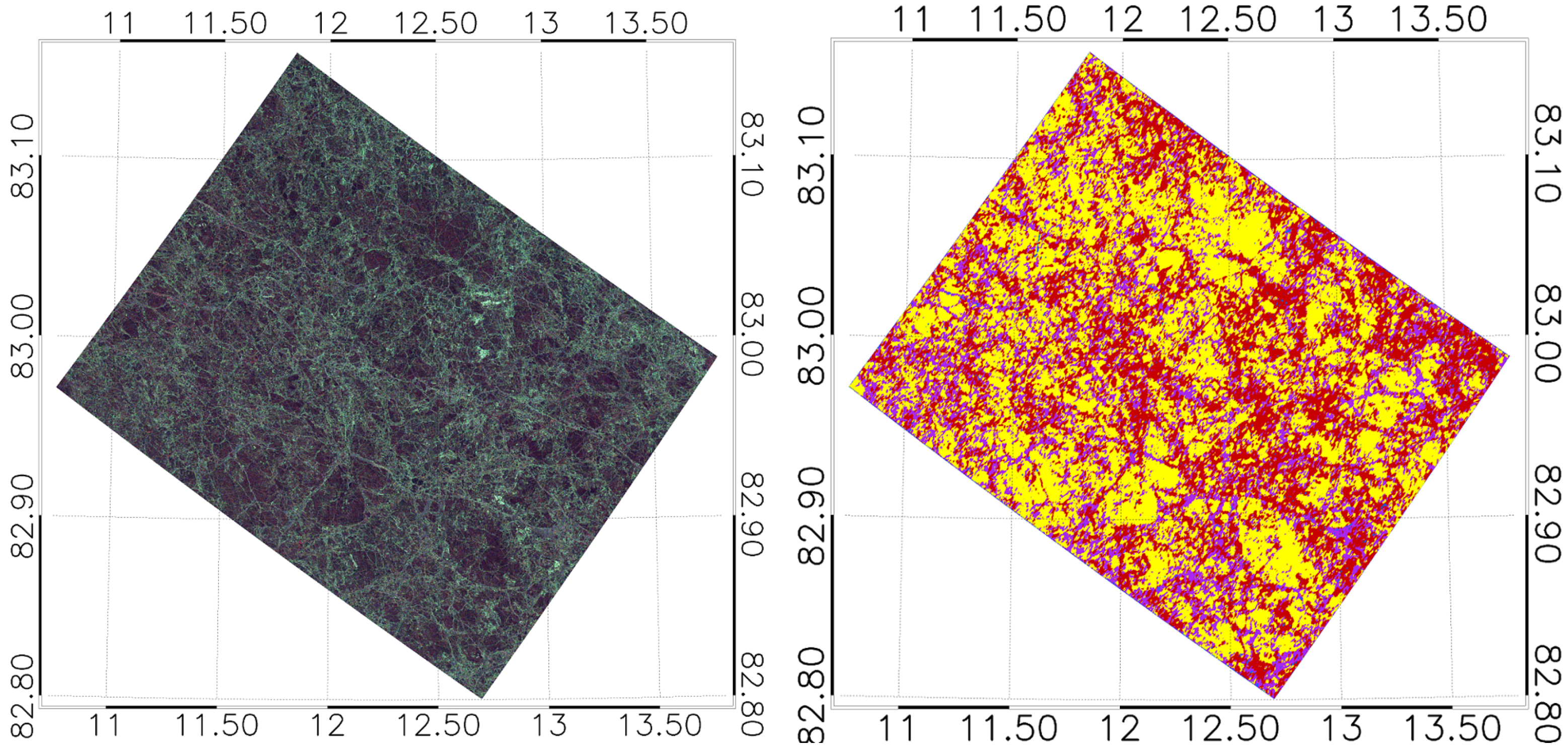
The distinction of all classes of ice are quite promising (see Table 6 ). Noting that both training and validation data are from the same ice situation (i.e., same time, location and incidence angle), our approach can be considered to be consistent in itself and stable in terms of the choice of the training data. When the ice situation does not vary significantly, our method can be expected to produce very reasonable results. To visually assess the classification, we juxtaposed all images in Figure 7 and Figure 8 (and Figure A1, Figure A2, Figure A3, Figure A4, Figure A5, Figure A6, Figure A7, Figure A8, Figure A9 and Figure A10 in the appendix for all other frames).

In Figure 1, one can see that only some of the frames for each acquisition day overlap. To ease the orientation when directly comparing the outcome of the classification results for the same ice structures, we included some examples in Figure 9 and Figure 10 with highlighted matching ice floe structures. Due to a lack of actual ground truth, we do not discuss in this juxtaposition which sensor offers the more plausible result. However, we do observe that for 19 April 2015 the TS-X image overstates the occurrence of RFYMYI at the expense of YI and SFYI, relative to the RS-2 classification (Figure 10). This behavior of the sensors appears to be reversed for the image of 23 April 2015 (Figure 9). We also note that the water portions that appear in the highlighted part of the (mid incidence angle range) RS-2 figure of 19 April 2015 (Figure 10) are practically absent in the (far range) TS-X image. The reversed behavior we observe in Figure 9, where the near range image (TS-X) shows detections of open water in the highlighted area whereas in the far range image there are no such detections. We also notice in the TS-X image of 23 April 2015 that RFYMYI (and also OW) tends to be overstated in the classification towards the vertical margins. Such tendencies we do not obersve in the far range TS-X image, nor any of the RS-2 images. So we summarize that for the locations of recognizably identical ice structures (black ellipse area and neighborhood in Figure 9 and Figure 10), we deem it justified to observe significant general match in the classified ice types with a possible incidence angle induced bias for certain ice types. This bias we observe similarly for X-band and C-band. The noticeable noise pattern (especially on the vertical margins) of the TS-X near range image of 23 April 2015 suggests the preferred use higher incidence angle acquisitions (i.e., above ${30}^{°}$). Such incidence angle biases certainly need to be addressed when establishing the classifier. This also stresses the necessity to establish a library of robust classifiers for different incidence angle ranges.

6. Conclusions

In this work, we conducted a thorough, quantitative comparison of spatially and temporarily near coincident quad-polarimetric images in X-band and C-band in terms of feature suitability for sea ice classification.

In order to judge in a rigorous and quantitative way on the suitability of different polarimetric features, we performed a mutual information based analysis of the data from all four acquisitions. Based on this analysis we arrived at the conclusion that, for our purposes, features involving eigendecomposition of the scatter coherency matrix $T_3$ do not provide informational benefit over features purely based on the covariance matrix $S_3$. Given the spatial and time correlation, in our findings we can preclude any impact of ice scene variability. The findings about the relevance and redundancy of particular features turned out to be similar for either of the SAR frequency bands. All extracted features were then used to train a neural network classifier. Numerical and visual analysis of results are rather promising in terms of providing inputs into the creation of operational ice charts. Future efforts will be devoted to refining the proposed methodology and testing our automated sea ice classification algorithm on pruned feature sets, in particular omitting eigendecomposition based features, excluding phase related information, or working with HH-VV information only. The generalizability and limitations of our method will be tested on a more extensive dataset and compared with ground truth.

References

1. Rigor, I.G.; Wallace, J.M. Variations in the age of Arctic sea-ice and summer sea-ice extent. Geophys. Res. Lett. 2004, 31, L09401. [Google Scholar] [CrossRef]
2. Maslanik, J.A.; Fowler, C.; Stroeve, J.; Drobot, S.; Zwally, J.; Yi, D.; Emery, W. A younger, thinner Arctic ice cover: Increased potential for rapid, extensive sea-ice loss. Geophys. Res. Lett. 2007, 34, 1–5, L24501. [Google Scholar] [CrossRef]
3. Stroeve, J.; Holland, M.M.; Meier, W.; Scambos, T.; Serreze, M. Arctic sea ice decline: Faster than forecast. Geophys. Res. Lett. 2007, 34, 1–5. [Google Scholar] [CrossRef]
4. Perovich, D.; Gerland, S.; Hendricks, S.; Meier, W.; Nicolaus, M.; Tschudi, M. Sea Ice; NOAA: Washington, DC, USA, 2014. [Google Scholar]
5. Karvonen, J. Operational SAR-based sea ice drift monitoring over the Baltic Sea. Ocean Sci. 2012, 8, 473–483. [Google Scholar] [CrossRef]
6. Kwok, R.; Spreen, G.; Pang, S. Arctic sea ice circulation and drift speed: Decadal trends and ocean currents. J. Geophys. Res.: Oceans 2013, 118, 2408–2425. [Google Scholar] [CrossRef]
7. Karvonen, J.; Vainio, J.; Marnela, M.; Eriksson, P.; Niskanen, T. A comparison between high-resolution EO-based and ice analyst-assigned sea ice concentrations. IEEE J. Sel. Top. Appl. Earth Obs. Remote Sens. 2015, 8, 1799–1807. [Google Scholar] [CrossRef]
8. Dierking, W.; Wesche, C. C-Band radar polarimetry—-Useful for detection of icebergs in sea ice? IEEE Trans. Geosci. Remote Sens. 2014, 52, 25–37. [Google Scholar] [CrossRef]
9. Hamidi, D.; Lehner, S.; König, T.; Pleskachevsky, A. On the sea ice motion estimation with synthetic aperture radar. In Proceedings of the 4th TerraSAR-X Meeting 2011, Oberpfaffenhofen, Germany, 14–16 February 2011; Volume Vortrags-Nr. CAL0166, pp. 1–10.
10. Liu, A.K.; Holt, B.; Vachon, P.W. Wave propagation in the marginal ice zone: Model predictions and comparisons with buoy and synthetic aperture radar data. J. Geophys. Res. 1991, 96, 4605–4621. [Google Scholar] [CrossRef]
11. Vachon, P.W.; Monaldo, F.M.; Holt, B.; Lehner, S. Ocean surface waves and spectra. In Synthetic Aperture Radar (SAR) Marine User’s Manual; Jackson, C.R., Apel, J.R., Eds.; NOAA NESDIS Office of Research and Applications: Washington, DC, USA, 2004; pp. 139–169. [Google Scholar]
12. Clausi, D.A. Comparison and fusion of co-occurrence, Gabor and MRF texture features for classification of SAR sea-ice imagery. Atmosphere-Ocean 2000, 39, 183–194. [Google Scholar] [CrossRef]
13. Clausi, D.A.; Zhao, Y. Rapid extraction of image texture by co-occurrence using a hybrid data structure. Comput. Geosci. 2002, 28, 763–774. [Google Scholar] [CrossRef]
14. Clausi, D.A.; Zhao, Y. Grey level co-occurrence integrated algorithm (GLCIA): A superior computational method to rapidly determine co-occurrence probability texture features. Comput. Geosci. 2003, 29, 837–850. [Google Scholar] [CrossRef]
15. Clausi, D.; Yue, B. Comparing cooccurrence probabilities and Markov random fields for texture analysis of SAR sea ice imagery. IEEE Trans. Geosci. Remote Sens. 2004, 42, 215–228. [Google Scholar] [CrossRef]
16. Ochilov, S.; Clausi, D. Operational SAR sea-ice image classification. IEEE Trans. Geosci. Remote Sens. 2012, 50, 4397–4408. [Google Scholar] [CrossRef]
17. Zakhvatkina, N.Y.; Alexandrov, V.; Johannessen, O.M.; Sandven, S.; Frolov, I. Classification of sea ice types in ENVISAT synthetic aperture radar images. IEEE Trans. Geosci. Remote Sens. 2013, 51, 2587–2600. [Google Scholar] [CrossRef]
18. Bogdanov, A.V.; Sandven, S.; Johannessen, O.M.; Alexandrov, V.Y.; Bobylev, L.P. Multisensor approach to automated classification of sea ice image data. IEEE Trans. Geosci. Remote Sens. 2005, 43, 1648–1664. [Google Scholar] [CrossRef]
19. Dierking, W. Sea ice monitoring by synthetic aperture radar. Oceanography 2013, 26, 100–111. [Google Scholar] [CrossRef]
20. Leigh, S.; Wang, Z.; Clausi, D. Automated ice-water classification using dual polarization SAR satellite imagery. IEEE Trans. Geosci. Remote Sens. 2014, 52, 5529–5539. [Google Scholar] [CrossRef]
21. Ressel, R.; Frost, A.; Lehner, S. A neural network based classification for sea ice types on X-band SAR images. IEEE J. Sel. Top. Appl. Earth Obs. Remote Sens. 2015, 8, 3672–3680. [Google Scholar] [CrossRef]
22. Kwok, R.; Rignot, E.; Holt, B.; Onstott, R. Identification of sea ice types in spaceborne synthetic aperture radar data. J. Geophys. Res.: Oceans 1992, 97, 2391–2402. [Google Scholar] [CrossRef]
23. Soh, L.K.; Tsatsoulis, C. Texture analysis of SAR sea ice imagery using gray level co-occurrence matrices. IEEE Trans. Geosci. Remote Sens. 1999, 37, 780–795. [Google Scholar] [CrossRef]
24. Karvonen, J.; Simila, M.; Makynen, M. Open water detection from Baltic Sea ice Radarsat-1 SAR imagery. IEEE Geosci. Remote Sens. Lett. 2005, 2, 275–279. [Google Scholar] [CrossRef]
25. Yu, Q.; Moloney, C.; Williams, F.M. SAR sea-ice texture classification using discrete wavelet transform based methods. In Proceedings of the 2002 IEEE International Geoscience and Remote Sensing Symposium, 2002, Toronto, Japan, 24–28 June 2002; Volume 5, pp. 3041–3043.
26. Dokken, S.; Håkansson, B.; Askne, J. Inter-comparison of arctic sea ice concentration using RADARSAT, ERS, SSM/I and in-situ data. Can. J. Remote Sens. 2000, 26, 521–536. [Google Scholar] [CrossRef]
27. Karvonen, J. A sea ice concentration estimation algorithm utilizing radiometer and SAR data. Cryosphere 2014, 8, 1639–1650. [Google Scholar] [CrossRef]
28. Shokr, M. Compilation of a radar backscatter database of sea ice types and open water using operational analysis of heterogeneous ice regimes. Can. J. Remote Sens. 2009, 35, 369–384. [Google Scholar] [CrossRef]
29. Dierking, W.; Skriver, H.; Gudmandsen, P. On the improvement of sea ice classification by means of radar polarimetry. In Proceedings of the 23rd EARSeL Symposium, Remote Sensing in Transition, Gent, Belgium, 2–5 June 2003; pp. 203–209.
30. Kwok, R.; Hara, Y.; Atkins, R.; Yueh, S.; Shin, R.; Kong, J. Application of neural networks to sea ice classification using polarimetric SAR images. In Proceedings of the Geoscience and Remote Sensing Symposium, Helsinki, Finland, 3–6 June 1991; Volume 1, pp. 85–88.
31. Drinkwater, M.R.; Kwok, R.; Winebrenner, D.P.; Rignot, E. Multifrequency polarimetric synthetic aperture radar observations of sea ice. J. Geophys. Res.: Oceans 1991, 96, 20679–20698. [Google Scholar] [CrossRef]
32. Winebrenner, D.P.; Farmer, L.D.; Joughin, I.R. On the response of polarimetric synthetic aperture radar signatures at 24-cm wavelength to sea ice thickness in Arctic leads. Radio Sci. 1995, 30, 373–402. [Google Scholar] [CrossRef]
33. Nghiem, S.; Kwok, R.; Yueh, S.; Drinkwater, M. Polarimetric signatures of sea ice: 1. Theoretical model. J. Geophys. Res.: Oceans (1978–2012) 1995, 100, 13665–13679. [Google Scholar] [CrossRef]
34. Nghiem, S.; Kwok, R.; Yueh, S.; Drinkwater, M. Polarimetric signatures of sea ice, 2, experimental observations. J. Geophys. Res.: Oceans (1978–2012) 1995, 100, 13681–13698. [Google Scholar] [CrossRef]
35. Tsatsoulis, C.; Kwok, R. Analysis of SAR Data of the Polar Oceans: Recent Advances; Springer: Berlin, Germany, 2012. [Google Scholar]
36. Yueh, S.H.; Kwok, R.; Lou, S.H.; Tsai, W.Y. Sea ice identification using dual-polarized Ku-band scatterometer data. IEEE Trans. Geosci. Remote Sens. 1997, 35, 560–569. [Google Scholar] [CrossRef]
37. Dierking, W.; Busche, T. Sea ice monitoring by L-band SAR: An assessment based on literature and comparisons of JERS-1 and ERS-1 imagery. IEEE Trans. Geosci. Remote Sens. 2006, 44, 957–970. [Google Scholar] [CrossRef]
38. Geldsetzer, T.; Yackel, J.J. Sea ice type and open water discrimination using dual co-polarized C-band SAR. Can. J. Remote Sens. 2009, 35, 73–84. [Google Scholar] [CrossRef]
39. Cloude, S.R.; Pottier, E. An entropy based classification scheme for land applications of polarimetric SAR. IEEE Trans. Geosci. Remote Sens. 1997, 35, 68–78. [Google Scholar] [CrossRef]
40. Wakabayashi, H.; Matsuoka, T.; Nakamura, K.; Nishio, F. Polarimetric characteristics of sea ice in the Sea of Okhotsk observed by airborne L-band SAR. IEEE Trans. Geosci. Remote Sens. 2004, 42, 2412–2425. [Google Scholar] [CrossRef]
41. Scheuchl, B.; Hajnsek, I.; Cumming, I. Sea ice classification using multi-frequency polarimetric SAR data. In Proceedings of the Geoscience and Remote Sensing Symposium, Toronto, Japan, 24–28 June 2002; Volume 3, pp. 1914–1916.
42. Lee, J.S.; Grunes, M.R.; Kwok, R. Classification of multi-look polarimetric SAR imagery based on complex Wishart distribution. Int. J. Remote Sens. 1994, 15, 2299–2311. [Google Scholar] [CrossRef]
43. Yang, F.; Gao, W.; Xu, B.; Yang, J. Multi-frequency polarimetric SAR classification based on Riemannian manifold and simultaneous sparse representation. Remote Sens. 2015, 7, 8469–8488. [Google Scholar] [CrossRef]
44. Atteia, G.; Collins, M.J. On the use of compact polarimetry SAR for ship detection. ISPRS J. Photogramm. Remote Sens. 2013, 80, 1–9. [Google Scholar] [CrossRef]
45. Dabboor, M.; Geldsetzer, T. Towards sea ice classification using simulated RADARSAT Constellation Mission compact polarimetric SAR imagery. Remote Sens. Environ. 2014, 140, 189–195. [Google Scholar] [CrossRef]
46. Moen, M.A.N.; Doulgeris, A.P.; Anfinsen, S.N.; Renner, A.H.H.; Hughes, N.; Gerland, S.; Eltoft, T. Comparison of automatic segmentation of full polarimetric SAR sea ice images with manually drawn ice charts. Cryosphere Discuss. 2013, 7, 2595–2634. [Google Scholar] [CrossRef]
47. Moen, M.A.N.; Anfinsen, S.; Doulgeris, A.; Renner, A.; Gerland, S. Assessing polarimetric SAR sea-ice classifications using consecutive day images. Ann. Glaciol. 2015, 56, 285. [Google Scholar] [CrossRef]
48. Praks, J.; Koeniguer, E.; Hallikainen, M. Alternatives to target entropy and alpha angle in SAR polarimetry. IEEE Trans. Geosci. Remote Sens. 2009, 47, 2262–2274. [Google Scholar] [CrossRef]
49. Nissen, S. Neural Networks made simple. Available online: http://www.software20.org (accessed on 10 May 2015).
50. Peng, H.; Long, F.; Ding, C. Feature selection based on mutual information criteria of max-dependency, max-relevance, and min-redundancy. IEEE Trans. Pattern Anal. Mach. Intell. 2005, 27, 1226–1238. [Google Scholar] [CrossRef] [PubMed]
51. Hajnsek, I.; Busche, T.; Krieger, G.; Zink, M.; Moreira, A. Announcement of Opportunity: TanDEM-X Science Phase; DLR: Oberpfaffenhofen, Germany, 2014. [Google Scholar]
52. Brekke, C.; Holt, B.; Jones, C.; Skrunes, S. Discrimination of oil spills from newly formed sea ice by synthetic aperture radar. Remote Sens. Environ. 2014, 145, 1–14. [Google Scholar] [CrossRef]
53. Thomsen, B.B.; Nghiem, S.; Kwok, R. Polarimetric C-band SAR observations of sea ice in the Greenland Sea. In Proceedings of the 1998 IEEE International Geoscience and Remote Sensing Symposium, Seattle, 6–10 July 1998; pp. 2502–2504.
54. Skrunes, S.; Brekke, C.; Eltoft, T. Characterization of Marine Surface Slicks by Radarsat-2 Multipolarization Features. IEEE Trans. Geosci. Remote Sens. 2014, 52, 5302–5319. [Google Scholar] [CrossRef] [Green Version]
55. Ressel, R.; Frost, A.; Lehner, S. Investigating the potential of different polarimetric features based on dual polarimetric TerraSAR-X data for automated sea ice classification. In Proceedings of the 2015 POLINSAR, Frascati, Italy, 26–30 January 2015; pp. 1–6.
56. Yu, L.; Liu, H. Feature selection for high-dimensional data: A fast correlation-based filter solution. In Proceedings of the 20th International Conference on Machine Learning (ICML-03), Washington, DC, USA, 21–24 August 2003; pp. 856–863.
Figure 1. Sea ice thickness on 15 April 2015 according to L3C SMOS data provided by ZMAW, Hamburg). Rectangles indicate the footprint of the acquisitions. The left image cluster was acquired on 19 April 2015 with temporal distance of 94 min, the right image cluster was acquired on 23 April 2015 with temporal distance of 59 min. The slim, long acquisitions are TS-X image (shown in white rectangles), the wider shorter ones are RS-2 images (shown in black rectangles).
Remotesensing 08 00198 g001
Figure 2. Images of different features for TS-X 23 April 2015, frame 1: (a) α ( d ) ; (b) α ( q ) ; (c) A ( d ) ; (d) A ( q ) ; (e) ε; (f) Δ ϕ ; (g) λ 1 ( d ) ; (h) λ 2 ( d ) ; (i) H ( q ) ; (j) H ( q ) ; (k) μ; (l) γ;, (m) ρ; (n) δ; (o) V a r Δ ϕ ; (p) s p a n ( d ) ; (q) s p a n ( q ) ; (r) τ.
Remotesensing 08 00198 g002
Figure 3. Images of different features for RS-2 23 April 2015, frame 1: (a) α ( d ) ; (b) α ( q ) ; (c) A ( d ) ; (d) A ( q ) ; (e) ε; (f) Δ ϕ ; (g) λ 1 ( d ) ; (h) λ 2 ( d ) ; (i) H ( q ) ; (j) H ( q ) ; (k) μ; (l) γ; (m) ρ; (n) δ; (o) V a r Δ ϕ ; (p) s p a n ( d ) ; (q) s p a n ( q ) ; (r) τ.
Remotesensing 08 00198 g003
Figure 4. Normalized mutual information for TS-X image of 23 April 2015, I ( Y 1 , Y 2 ) / H ( Y 1 ) H ( Y 2 ) . Features are: 1: γ, 2: Δ ϕ , 3: ρ, 4: ε, 5: μ , 6: τ , 7: s p a n ( q ) , 8: δ, 9: H ( q ) , 10: A ( q ) , 11: α ( q ) , 12: s p a n ( d ) , 13: H ( d ) , 14: A ( d ) , 15: α ( d ) , 16: λ 1 ( d ) , 17: λ 2 ( d ) , 18: V a r Δ ϕ .
Remotesensing 08 00198 g004
Figure 5. Normalized mutual information for RS-2 image of 23 April 2015, I ( Y 1 , Y 2 ) / H ( Y 1 ) H ( Y 2 ) . Features are: 1: γ, 2: Δ ϕ , 3: ρ, 4: ε, 5: μ , 6: τ , 7: s p a n ( q ) , 8: δ, 9: H ( q ) , 10: A ( q ) , 11: α ( q ) , 12: s p a n ( d ) , 13: H ( d ) , 14: A ( d ) , 15: α ( d ) , 16: λ 1 ( d ) , 17: λ 2 ( d ) , 18: V a r Δ ϕ .
Remotesensing 08 00198 g005
Figure 6. (Top Left) Plot of the domain of admissible ( p 1 ( q ) , p 2 ( q ) ) pairs. (Top Right) plot of pairs ( p 1 ( q ) , p 2 ( q ) ) , where the relative deviation | δ H ( q ) | / H 10 % . (Bottom): relative deviation | δ H ( q ) | / H .
Remotesensing 08 00198 g006
Figure 7. (Left) Geocoded Pauli RGB composite (Red: HH-VV Green: HV+VH Blue: HH+VV) of the TS-X acquisition on 23 April 2015, frame 1; (Right) ice classification. Blue: open water/nilas (OW), purple: young ice (YI), yellow: first year ice (SFYI), red: rough first year ice/multi-year ice (RFYMYI).
Remotesensing 08 00198 g007
Figure 8. (Left) Geocoded Pauli RGB composite (Red: HH-VV Green: HV+VH Blue: HH+VV) of the RS-2 acquisition on 23 April 2015, frame 1; (Right) ice classification. Blue: open water/nilas (OW), purple: young ice (YI), yellow: first year ice (SFYI), red: rough first year ice/multi-year ice (RFYMYI).
Remotesensing 08 00198 g008
Figure 9. Comparison of classification results. For orientation, black ellipses indicate same ice structures. (Left) ice classification of TS-X acquisition on 23 April 2015; (Right) ice classification of RS-2 acquisition on 23 April 2015. Blue: open water/nilas (OW), purple: young ice (YI), yellow: first year ice (SFYI), red: rough first year ice/multi-year ice (RFYMYI).
Remotesensing 08 00198 g009
Figure 10. Comparison of classification results. For orientation, black ellipses indicate same ice structures. (Left) ice classification of TS-X acquisition on 19 April 2015; (Right) ice classification of RS-2 acquisition on 19 April 2015. Blue: Open Water/nilas (OW), purple: Young Ice (YI), yellow: first year ice (SFYI), red: rough first year ice/multi-year ice (RFYMYI).
Remotesensing 08 00198 g010