1. Introduction
In a paper recently published in this journal, Sun and Schulz found that the addition of the thermal band in Landsat improves the overall accuracy (OA) of land cover classification [
2]. In a subsequent comment, Johnson [
3], surprised by the high accuracy they obtained (up to 99% OA with four classes) and by the contrast between their findings and those of other recent research, correctly identified a flaw in the accuracy assessment, namely the lack of independence between training and validation pixels. In essence, the authors, who had delineated a number of individual polygons of each class for use as ‘ground truth’ (446 polygons in total, of 5 ha mean size), were separating reference pixels into training (90%) and validation (10%) in a way that placed most validation pixels adjacent to training pixels, which in the case of the thermal band meant that they had overlapping footprints. In their response to Johnson’s comment, Sun and Schulz [
4] acknowledged this problem and implemented the solution suggested by Johnson; that is, reserving all the pixels of some of the reference polygons for validation, so that training and validation pixels would be distant from each other. With the corrected method, OA decreased about 5%, but the inclusion of thermal band still improved classification performance.
Intrigued by the rarity of a formal comment on the accuracy assessment of a paper about land cover mapping, a topic in which I am interested (e.g., [
5,
6]), I read the original paper, comment, and response [
2,
3,
4]. Alas, I came to the conclusion that there were still some issues, and felt that if they were left undiscussed, one could be left with the impression that the accuracy assessment in [
4] was correct. I contacted both the authors and the editors. The former kindly provided me with further explanations on their methods, shared with me part of their data, and gave me permission to use them in a comment. The latter welcome my inquiry and encouraged me to write a comment.
In this comment, I point out and discuss those further issues, following the good-practices framework by Olofsson
et al. [
1], which uses the classical partition of accuracy assessment into sampling design, response design, and analysis [
7]. But first, two caveats: (i) for the sake of brevity, I will focus my comment on the accuracy assessment of the level 2 classification (seven classes: agriculture; grassland; built-up; deciduous, conifer and mixed forests; and water) of the July 2013 Landsat-8 image classification for the 288 km
2 study area based on the k-NN method with all 10 bands, which I obtained from the authors; and (ii) by pointing at the issues, I do not wish to lay any blame on the authors; on the contrary, from our interactions, I can attest to their candor and openness. Furthermore, I could very well find flaws in some accuracy assessments I’ve done in the past, so my intention is calling for more rigor in our accuracy assessments.
2. Issues Regarding the Sampling Design
The sampling design is the protocol for selecting the subset of pixels where the land cover class is ascertained by more accurate means, which forms the basis of the accuracy assessment. Olofsson
et al. [
1] strongly recommend that sampling design be probability based, such as simple random and stratified random, so that appropriate formulas for estimating statistical parameters can be used. Unfortunately, the authors of [
2] used a purposive sampling protocol where they strove to delineate areas so that: (i) they looked homogeneous in the Landsat image; (ii) they were fully inside one of the polygons of the reference map they used for assigning labels; (iii) they had a size in the range 1–30 ha; and (iv) they were evenly distributed across the study area and across classes. In doing so, the authors forfeited the possibility of producing confidence intervals for the area totals of each land cover class or for their estimated overall accuracy. This is because the inclusion probability (of selecting a given pixel as part of the validation sample) is largely unknown for any given pixel in the study area, whereas inclusion probabilities are employed as inverse weights in the estimation of those parameters, even though they may not appear explicitly in the formulas [
1]. The outcome of the purposive sampling protocol can be seen as limiting the sample frame (
i.e., the set of selectable pixels) to those within the delineated reference polygons, in which case the inclusion probability in each run of the 10-fold cross-validation is 10% for all pixels inside. However, pixels outside the reference polygons had a zero inclusion probability; therefore, the results of the accuracy assessment cannot be validly extrapolated to 92% of the study area not covered by reference polygons. Put another way, purposive selection of reference areas is warranted for training the classifier, but it drastically reduces the usefulness of the classifier performance statistics as measures of accuracy for a map derived from that classifier.
Notwithstanding, this issue alone does not forfeit the authors’ conclusion that the addition of the thermal band improves the performance of the tested classifiers. We just don’t know how much this improvement increases the accuracy of the resulting maps. However, this would have been possible if instead of a sampling approach the authors had resorted to a census, which indeed they could because the land cover map they used for labeling the reference polygons was actually available for their entire study area. That is, they could have still used the reference polygons they delineated for training, but for validation they could have used all pixels outside them (but see the next section).
3. Issues Regarding the Response Design
The response design includes all steps, procedures and materials leading to the assignment of a reference land cover class in each of the selected sampling units (
i.e., in the validation pixels). Contrary to what the remote sensing jargon ‘ground truth’ conveys, these reference values are themselves subject to uncertainty and errors that should be accounted for and discussed [
1]. For example, to label their reference polygons, the authors of [
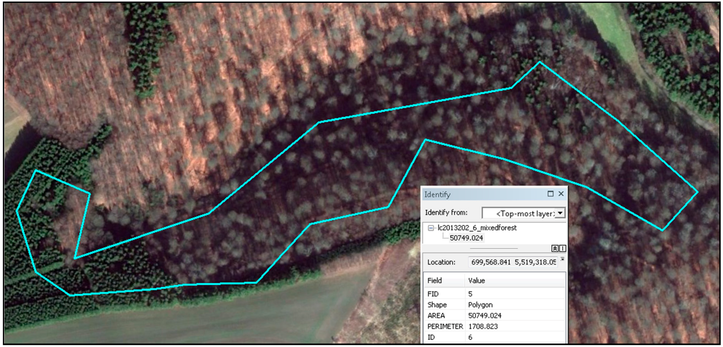
2] used the OBS map (Occupation Biophysique du Sol, a polygon inventory of land cover and biotopes in Luxembourg derived from photo-interpretation of aerial photography of 1:10,000 scale). Even the best maps contain errors, and a possible example is shown
Figure 1, which corresponds to a reference polygon that was assigned to the mixed forest class. In contrast, in the image acquired on 1 March 2011 that currently appears in Google Earth, most trees seem to be deciduous. I speculate that a possible source of this error is that the photography used for the OBS map was leaf-on, plus the polygon corresponds to a shady hillside that would yield a darker tone in the leaf-on ortho-photo, suggesting some trees were conifer.
There were some apparent errors also for the grassland class, where some of the reference polygons had clear signs of agricultural practices (not shown). Whenever faulty reference polygons are selected for validation in the corrected method of [
4], all pixels inside them count as correctly classified in the confusion matrix, whereas in reality most are wrong (an exception in the faulty polygon of
Figure 1 are the few 30-m pixels corresponding to the uppermost corner of the shape, which indeed appears to be mixed forest). I asked the authors if they had used Google Earth to verify the label of reference polygons; they said that only in very few instances where the appearance in the Landsat image was doubtful. While it is warranted to use the same Landsat imagery that will later be classified for delineating homogeneous training areas, it would have been preferable to systematically ascertain the assigned class by inspecting every reference polygon in Google Earth, because it has submetric resolution imagery available for the study area and it allows overlaying polygons in
kml format. If after this exercise too many errors are detected in the reference map (or if there are too many gaps of a different land cover inside the polygons that were not captured in the map due to minimum mapping unit constraints), then the census approach would be neither practical nor reliable, and a probability-based sampling design would be necessary. For example, after running a 3 by 3 majority filter on the output raster, 50 pixels of each class could be randomly selected from a list, and then assigned a reference class based on the appearance in Google Earth of the terrain encompassed within a 90-m square centered at the pixel.
4. Issues Regarding the Analysis
The final component of the assessment is the analysis of the agreement between reference and map in validation pixels so as to derive accuracy statistics. A common error in the analysis is to use pixel counts instead of proportions to estimate accuracy, which the authors seem to have done (given the confusion matrices and respective overall accuracies they shared with me). Using raw pixel counts assumes that all the validation pixels have the same inclusion probability and thus the same weight, whereas this is seldom the case. For example, if we randomly selected 50 pixels of each class and the proportion
Wi of area mapped as class
i differed among classes, then the sampling intensity we would be applying to each class is obviously different. If a predominant class (hence undersampled when compared to others) happens to be the class with most errors, or if a less common (hence oversampled) class is also the most accurately mapped, then we are overestimating overall accuracy. This doesn’t seem to be of concern in the case of [
2], because the proportion
wi. of validation pixels belonging to class
i is close to
Wi given that the authors took care that the total area of reference polygons of each class was proportional to that in the OBS map. But in the ‘polygon cross-validation’ of [
4], the
wi. can differ considerably from their respective
Wi depending on what particular reference polygons get selected for validation in each run. See [
1] for an explanation of how to correctly estimate the proportion of map area that has class
i in the map and class
j in the reference, for each possible pair (
i,
j) including (
i,
i).
Another aspect that is often neglected is that unless the validation set contained the entire population of pixels in our map, the accuracy estimates we derive from the confusion matrix are subject to uncertainty. Different samples will yield different results; consequently, we must provide a range within which the true value (
i.e., that which would be obtained from a census of all pixels in the map) is likely to fall, which is known as confidence interval. The latter can be derived if the sampling design is probability based, that is, if the inclusion probability is greater than zero for all pixels in the map and can be known. Olofsson
et al. [
1] recommend stratified random sampling as a good choice, because it is practical, easy to implement, and affords the option to increase the sample size. The latter is desirable in situations where there are requirements such that “the producer must defend in a statistically valid manner that the overall accuracy of the map exceeds 75% with a 95% confidence level”, which implicitly dictates the sampling effort required to achieve that confidence once the estimate is available (the 75% is the lower limit of the confidence interval).
5. Conclusion and Recommendations
There were other relevant issues in the accuracy assessment of [
2] beyond that pointed out in [
3]. Regrettably, I suspect this is more the norm than the exception: I speculate that if we randomly picked a sample of recent articles describing land cover mapping efforts and scrutinized their accuracy assessments, the majority would have some issue, or at least incomplete information to judge if there are issues. I do not have data to support this claim other than my own experience as reader and reviewer, hence I may well be wrong. However, I feel we all need to make further efforts to ensure that the accuracy assessments we perform or review are scientifically defensible. Olofsson
et al. [
1] make excellent recommendations in their summary section, to which I would like to add some specific suggestions to authors, reviewers and editors. Authors should strive to provide all relevant detail, positive or negative, that would allow readers to judge the merit of their contribution; an important part of that is the accuracy assessment. Reviewers should check that enough detail is provided about sampling design, response design and analysis, and demand rigorously computed confidence intervals for the accuracy estimates. Also, editors could encourage authors to share the data used in the accuracy assessment as supplementary material, especially the location of the samples used to populate the confusion matrix. The additional effort this would require is just a small price we would all have to pay to enhance the scientific credibility of our discipline.


