Impact of MODIS Quality Control on Temporally Aggregated Urban Surface Temperature and Long-Term Surface Urban Heat Island Intensity

Abstract

Surface Urban Heat Island (SUHI) is a phenomenon of high spatial and temporal variability. However, studies that investigate urban land surface temperature (LST) observed in different seasons frequently utilize a single satellite measurement and do not incorporate temporal composites. Temporally aggregated data increase clear sky coverage, which is important in many aspects of urban climatology. However, it is critical to account for possible errors and quality of the data that are utilized. The objective of this paper is to analyze the impact of MODIS Quality Control (QC) and the view angle on temporally aggregated urban surface temperature and long-term SUHI intensity. To achieve this, a weighted arithmetic mean was utilized whose weights were based on the view angle of satellite observation and the MODIS QC flags; namely, LST retrieval errors and emissivity errors. In order to investigate the impact of the MODIS QC on long-term LST composites, five exponential powers were applied to weights during the temporal aggregation process, resulting in five thresholds of best quality pixel promotion. It was found that there are significant differences between temporal composites that take into account the MODIS QC and the view angle and those that do not (obtained by means of a simple arithmetic mean with no weights applied), in terms of spatial distribution and density distribution of urban and rural LST. The differences were more distinctive in spring or daytime cases than in autumn or nighttime cases. The impact of the MODIS QC and the view angle on temporal composites was highest in the city center. Ten SUHI indicators were utilized. It was found that the impact on long-term SUHI intensity is weaker than on the spatial pattern of LST and that SUHI indicators are inconsistent.

1. Introduction

The urban heat island (UHI) is a direct consequence of anthropogenic land transformation [1]. It is a phenomenon that describes a local perturbation in the three-dimensional (3D) temperature field of the atmosphere in the vicinity of urban agglomerations. It is typically referred to as the difference between air temperatures observed in urban and rural areas. Air temperature is a parameter that is most apparent to the inhabitants. It is recorded with high frequency and accuracy by meteorological weather stations. Unfortunately, in most cases, the density of the meteorological network is not sufficient to characterize the spatial pattern [2]. By contrast, satellite instruments are capable of instantaneous measurement of land surface temperature (LST) over vast areas, which represents their greatest advantage over other observational techniques.

Voogt and Oke proposed the term “Surface Urban Heat Island” (SUHI) for UHI, indicating the difference between urban and rural land surface temperature, and addressed methodological questions concerning SUHI that had been raised previously by Roth [3,4]. Despite complex interactions across scales, the physical coupling of surface and atmosphere makes the identification of SUHI a logical path to identifying mitigation strategies for UHI [5]. Using remote sensing to study SUHI can improve the understanding of the spatial-temporal variability of physical processes that influence the long-term urban climate [6]. In general, raised temperatures in urban areas, compared to surroundings, are easily observed on satellite thermal imagery, but the differentiation between “urban” and “rural” remains diverse and confusing [7].

Land surface temperature is key to understanding the interactions and energy fluxes between the Earth’s surface and the atmosphere [8,9]. Hence, there have been significant efforts put into achieving an understanding of LST patterns over urban and rural areas [10,11,12,13,14,15]. Furthermore, air temperature is strongly dependent on LST [16]. Thus, the linkage between air and surface temperature in urban areas has also been studied [17,18,19,20]. Moreover, one of the most frequently investigated relationships that describes an anthropogenic modification of natural surfaces is the relationship between an impervious surface area (ISA) and surface temperature [8,21,22,23,24]. Also, the relation between indirectly described human activity or population characteristics and LST, have also been extensively studied, e.g., population density [25,26]; socioeconomic patterns (inter alia, the number of families [25]); human settlement characteristics, including household income or a population’s race [27]; poverty, ethnic minorities, high crime risk, and education [28]; road density [29]; risk of heat stress [30,31]; and mortality ratio [32]. Remotely-sensed night lights offer another interesting parameter that has been used to allocate many aspects of human activity in spatial terms [5,33,34,35,36,37]. However, most of those papers have utilized single observations without constructing temporal composites.

Studies focused on the city of Warsaw have utilized single AVHRR [38], Landsat [39,40,41], or MODIS [31,42] observations. The study in [38] does not describe any specific features of SUHI. It is focused only on the problem of LST retrieval. In [31], a single MODIS LST and NDVI products are utilized in order to analyze a potential risk of high temperature exposure during a heat wave event. Districts that had the highest LST and lowest NDVI values were identified as the most vulnerable to heat stress. The only published papers that give more insight into the spatial pattern of LST and SUHI are [31,40,41,42].

The study in [40] utilized two Landsat TM images for 15 July 1987 and 16 August 1993, as well as one in the transitional season (2 April 1990). Similarly, the study in [41] utilized two summer Landsat TM images (13 June 1987 and 15 July 1987) and one in the transitional season (3 October 1987). The study in [39] utilized one summer Landsat TM image (11 July 1987). Unfortunately, by employing a different approach, a different instrument with higher spatial resolution, and a different time span, the obtained values of SUHI are not comparable to this study. However, the aforementioned studies give some understanding of the spatial patterns of LST in Warsaw.

The study in [42] was focused on the comparative analysis of spatial patterns of LST and SUHI intensity in three Polish cities (Warsaw, Cracow, and Wroclaw) during a heat wave event. There were two MODIS LST observations utilized: one for the daytime case and the other for the nighttime case. The study showed that the daytime intensity of SUHI in Warsaw may reach 2.2 °C (indicator “urban mean—other”) and 14.6 °C (indicator “range”), while nighttime SUHI intensity was weaker: 2.1 °C (“urban mean—other”) and 6.2 °C (“range”). In terms of the spatial pattern, the River Vistula was visible in the daytime image but not visible in the nighttime image. Central districts were much hotter than less urbanized ones in both cases. In addition, probability density functions (PDFs) were prepared, which described urban and rural areas separately. In the nighttime case, LST values had a smaller range than in the daytime case (9 °C and 17 °C). In the nighttime case, the PDF function for urban areas had two maxima, while rural areas during nighttime as well as all rural and urban areas in the daytime case had one maximum.

There are no peer-reviewed papers published that can give comprehensive information about the long-term spatial pattern of LST or SUHI intensity in the city of Warsaw. This study is the first of its kind.

SUHI is a phenomenon that is not only concerned with high spatial variability, but also with high temporal variability [43]. However, studies that investigate urban LST observed in different seasons frequently utilize a single satellite measurement and do not incorporate temporal composites [44]. Since surface temperature is influenced by synoptic conditions (e.g., wind and humidity), such an approach may lead to discrepancies. In order to avoid such uncertainties, it is advisable to use temporal composites.

Air temperature is typically observed in situ by automatic stations on a round-the-clock basis. Since the availability and quality of such measurements are, in general, not hampered by synoptic conditions, it is quite straightforward to derive mean statistics in order to describe the long-term behavior of the UHI phenomenon [45,46,47,48,49]. In spite of the fact that satellite remote sensing techniques give a full spatial pattern over a vast area, such measurements are strictly limited to cloudless conditions during a satellite overpass [50]. This significantly reduces the availability and applicability of satellite LST observations, especially over areas and seasons with high cloudiness occurrence. Consequently, calculation of long-term composites is of special interest to investigators.

Analysis of long-term land surface temperature data composites is important in many aspects of urban climatology, i.e., seasonal and annual LST variability investigations, development of UHI mitigation strategies, or composition of mean climatologies for modeling purposes. Recently in this field, Hu and Brunsell [6] studied the impact of temporal aggregation of LST data for SUHI monitoring in Houston, Texas. The authors incorporated 10 years of MODIS Terra and Aqua observations and found that SUHI intensities are notably enhanced in the daytime compared with the nighttime, with an increasing trend with larger composite periods, and that temporal aggregation processes do indeed impact the spatial pattern of LST. Quan et al. [51] applied the Gaussian volume model to derive the centroid of the UHI in Beijing, based on daily MODIS LST products, from the period 2000 to 2012, and analyzed daily, monthly, and annual variability. In [52], its authors propose a procedure to extract thermal patterns for the quantitative analysis (more than 3000 images) of satellite-derived LST maps. Weng and Fu [43] characterized the annual and seasonal surface temperature behaviors during the period from 2000 to 2010 in the city of Los Angeles by employing an annual temperature cycle model. Clinton and Gong [5] used all MODIS Terra and Aqua images from the year 2010 to characterize the urban surface heat differential (SUHI and its inversion SUHS—Surface Urban Heat Sinks) and identify urban environmental variables, which are globally meaningful for diagnosing and predicting SUHI and SUHS. In this study, the authors have only used pixels with LST retrieval error less than 1 K.

Composite data directly increase the clear sky coverage across urban and rural regions, which is beneficial for SUHI studies; however, many papers do not consider the possible errors caused by composite processes [6]. Most of the previous studies have explored urban thermal patterns over space and time using a limited number of clear sky images or by removing cloud-contaminated pixels. The limitation in the number of image scenes prevents the derivation of long-term LST climatology for a particular region. Moreover, simply eliminating cloudy pixels inevitably obscures the spatial and temporal patterns of LST [43]. Although previous investigations of MODIS multi-temporal urban LST patterns account for cloud contamination (e.g., [6,51,52]), they fully or partially neglect the spatial pattern of LST retrieval or emissivity errors, which may influence the quality of resulting LST patterns and calculated SUHI intensities.

Off-nadir satellite remote sensing observations oversample vertical structures. Moreover, urban areas show significant thermal anisotropy. Consequently, off-nadir views may yield temperatures that are warmer or cooler than nadir views; this depends on the view direction relative to the solar position [3]. The difference between the LST measured in nadir and off-nadir observations can be as large as 5 K for bare soil and even 10 K for urban areas [53]. Hence, angular dependencies are particularly important when applying observations from sensors with a wide field of view (FOV) to studies focused on urban areas. A MODIS view angle of ±55° results in high temporal resolution. However, a nadir view of the target area is available only once every 16 days.

With such wide scan angle (equivalent to a 68° view zenith angle of the Earth’s surface), the MODIS swath spans about 2 h in the local time of the observation at the equator [54]. Hence, MODIS observations of urban areas can be acquired from different sides (west or east) of the vertical axis of buildings with a different solar zenith angle. As the scattering properties of the atmosphere are directional, views towards the sun will be affected by quite a different scattering than views away from the sun at the same viewing angle [55]. In terms of wide view angles, the LST is not only angle-dependent but also depends on emissivity [56].

Therefore, when constructing a temporal composite of urban LST, it seems unjustified to treat nadir and off-nadir satellite observations equally. However, most of the long-term LST studies that utilize MODIS images do not take into account angular dependencies [6,51,52]. In [52], scene view angles higher than 45° were neglected. However, all included scenes were treated equally, without any weighting for the off-nadir view angle. In addition, some studies utilize temporal composites, such as MOD/MYD11A2 products (which represent an eight-day mean LST), without any accounting for dependencies between the 3D structure of urban areas and off-nadir observations. Adjacent LST pixels in MOD11A2 products are obtained during different cloudiness conditions and with different view angles. Such an approach may lead to discrepancies (e.g., in [57], eight products were used—four per month). In this study, we account for dependencies between the 3D structure of urban areas and off-nadir observations by applying appropriate weights, which are based on the acquisition angle (see Section 2).

The primary objective of this paper is to analyze the impact of the MODIS QC and the view angle on the temporal composites of LST in Warsaw (Poland). This was achieved by estimating the mean intensity of the SUHI phenomenon in Warsaw in the transitional seasons (spring and autumn) by obtaining the most representative (by a single sensor as much possible) mean LST image for the previous 15 years. This objective was achieved by an investigation into the influence of different temporal aggregation techniques of LST data on the spatial distribution of LST and several indicators of SUHI [18,57]. Given the nature of remote sensing observations and typical cloud conditions in the target city, the intention behind the approach was to promote observations that represented the highest quality of LST. This was achieved by utilizing a weighted arithmetic mean whose weights were based on the MODIS QC metadata [58]; namely, the view angle, LST retrieval errors, and emissivity errors.

2. Data and Methods

2.1. Study Area

The city of Warsaw has an area of 517.24 km². There are about 1,700,000 inhabitants in the city, but the population in agglomeration exceeds 2,500,000 [59]. The average population density is 3324 persons/km². Warsaw is located in the central part of Poland, at 78 to 121 m above sea level. The biggest river in Poland, the Vistula, flows through Warsaw. The city has 18 administrative districts.

Since Warsaw has a transitional climate, synoptic conditions may be very different from year to year. According to the Climate Atlas of Poland [60], the average annual number of cloudy days (more than seven oktas) in the years 1971 to 2000 was between 140 and 150 (in winter, it was between 50 and 60 days), while the average annual number of cloudless days (less than two oktas) was between 30 and 40 (in winter, it was five to 10 days). In March, the average air temperature is 2.5 to 3 °C, while it is 13 to 13.5 °C in September (these months correspond to the spring and autumn equinox). The annual mean total sunshine duration is about 1650 h.

Zalew Zegrzyński Lake is located north of Warsaw. Given its proximity to the Warsaw agglomeration (about 10 km) and size (33 km²), it was used as a reference to calculate one of the SUHI intensity indicators (“urban mean—water”). In order to analyze the entirety of Warsaw’s agglomeration, including nearby rural areas, we set a buffer zone around the city. It included areas within about 10 km in each direction from the edges of Warsaw’s administrative borders. The buffer zone was used to calculate the indicator “urban mean—other”.

2.2. Data

Since transitional seasons (spring and autumn) in Poland typically have high variability of synoptic conditions, we utilized all available MODIS Terra MOD11A1 (collection 5) products that represent gridded daily LST from 2000 to 2014. For each case analyzed, we chose 32 consecutive MOD11A1 products that corresponded with the spring and autumn equinox (approximately 16 products before and 16 after). To sum up, 1920 rasters were taken into account. MODIS Aqua observations were neglected due to a different time of satellite overpass and a different consequent stage of SUHI, as well the unavailability of observations for the period 2000 to 2002. Moreover, in order to account for severe cloud contamination, we neglected rasters that had a number of available LST pixels lower than 60%. In addition, unreliable LST values (lower than −15 °C and more than 25 °C) were neglected. In order to avoid unrealistic LST values, for each three subsequent pixels in the row of a raster, the difference between first and second or second and third were required to be lower than 12 °C, otherwise “0” was the weight applied to the second pixel out of three. Such a condition is reasonable given the coarse resolution of MODIS observations in thermal channels and the characteristics of the target area. The weight “0” was applied when there was no LST value in the MOD11A1 layers or when a pixel was acquired from a view angle higher than 40° [61]. Moreover, MODIS scientific datasets (SDS) that consist of LST values and QC flags are not consistent. It happens (about 5%–10% in each season) that a MODIS QC “mandatory flag” indicates that LST is not produced for a specific pixel; meanwhile, on the appropriate layer, this pixel has an LST value available. To account for this inconsistency, if the weight as indicated by the emissivity error flag or LST retrieval error flag was greater than three in this case, it was reduced to 3. The processing chain is explained in detail in Figure 1.

Table 1. Data quality statistics expressed as calculated weights.

Weights Type	Weight Value	Autumn Day	Autumn Night	Spring Day	Spring Night	Data Stratification
Rasters included:		236	254	176	211	Description:
Weights based on α view angle	0	52%	51%	54%	58%	−40° < α > 40°
	1	6%	6%	5%	6%	−40° > α > −35°; 35° > α > 40°
	2	8%	7%	8%	4%	−35° > α > −30°; 30° > α > 35°
	3	7%	10%	8%	8%	−30° > α > −25°; 25° > α > 30°
	4	3%	4%	2%	5%	−25° > α > −20°; 20° > α > 25°
	5	9%	8%	10%	8%	−20° > α > −15°; 15° > α > 20°
	6	4%	6%	3%	3%	−15° > α > −10°; 10° > α > 15°
	7	6%	6%	5%	4%	−10° > α > −5°; 5 > α > 10°
	8	5%	3%	5%	4%	−5° > α < 5°
Weights based on LST retrieval errors	0	22%	12%	23%	21%	LST not available
	1	0%	0%	0%	0%	Average emissivity error > 0.04
	2	1%	0%	1%	0%	Average emissivity error ≤ 0.03
	3	25%	26%	28%	27%	Average emissivity error ≤ 0.02
	4	4%	5%	3%	5%	Average emissivity error ≤ 0.01
	5	48%	56%	45%	48%	Good quality, not necessary to examine more detailed QC
Weights based on emissivity errors	0	22%	12%	23%	21%	LST not available
	1	3%	2%	3%	3%	Average LST error > 3 K
	2	2%	2%	2%	2%	Average LST error ≤ 3 K
	3	11%	13%	10%	10%	Average LST error ≤ 2 K
	4	0%	0%	0%	0%	Average LST error ≤ 1 K
	5	63%	71%	62%	65%	Good quality, not necessary to examine more detailed QC

shows the weight distributions applied in the study.

The errors shown in Table 1 reveal some abnormal distribution. However, inconsistencies in the MODIS QC flags were already documented [62]. It is noted that 50% of pixels in each case that was analyzed were acquired with very high view angles exceeding 40°, while lower view angles, depending on the case, were observed for 2% to 10% of pixels. In the case of weights based on LST retrieval errors, the majority of pixels (45%–56%) have the highest weight applied, the second biggest group of pixels have weight “3” applied (26%–28%), and 12%–23% of pixels have no LST available. The lowest amount of pixels have weights “2” and “4” applied, and almost no pixels have weight “1” applied. In the case of emissivity errors, the distribution of weights is similar to those based on LST retrieval errors. However the majority of pixels have the highest weight of “5” applied (62%–71%), while there were no pixels with weight “4” applied.

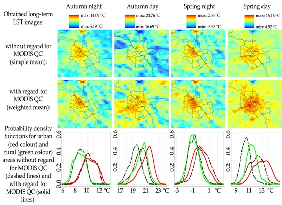
2.3. Estimation of 15-Year Mean LST Rasters

In order to analyze the impact of the MODIS QC on temporally aggregated LST, there were two types of composition prepared:

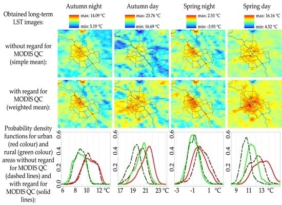
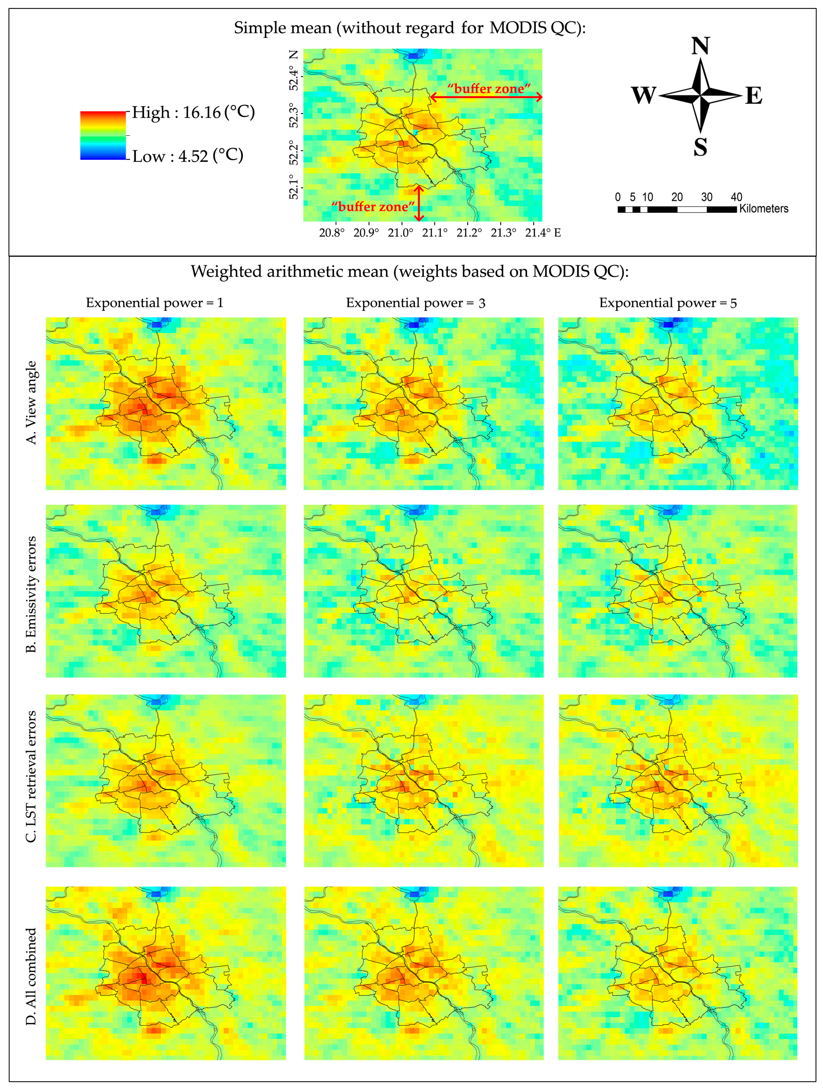
• The “first” type of LST composition was built by means of a simple arithmetic mean with no regard for any metadata; and,
• The “second” type of LST composition was built by means of a weighted arithmetic mean whose weights were based on the MODIS QC metadata.

Figure 1 explains the processing chain for a single case in detail. In order to obtain a set of long-term mean rasters, the first operation was to crop each MOD11A1 product into boundaries of AOI (area-of-interest). The next step was to check the fraction for available LST observations within the AOI; if less than 60% of pixels was available, the given raster was removed from further processing. For the rasters that passed the first condition, a loop was initiated that was concerned with all the available pixels on a given raster. In order to obtain an averaged raster by means of the first type of composition (simple mean), for a given location (pixel), all available observations on each raster were taken into account. A final raster was built by means of a simple mean without taking account of the MODIS QC.

In the case of the second type of composition, LST observations were not only taken into account, but also the available metadata concerning the quality of pixels. Each MOD11A1 product consists of 12 layers (SDS). There are two types of error indicated by the MODIS QC: LST retrieval errors and emissivity errors. The view angle was also taken into account. Appropriate weights were built on the gradual magnitude of two types of error (six thresholds), as well as on the increasing view angle (nine thresholds). Consequently, four types of final averaged rasters were built. Each was built by weighted arithmetic mean, where weights were of four different types based on LST retrieval errors, on emissivity errors, on view angle, and on the sum of all weights combined.

In order to bring out pixels with the highest quality indicated, increasing exponential powers (one to five) were applied to all types of weight during the composition process. Each pixel on each raster had appropriate weights applied, and a final 15-year averaged LST image was built by means of a weighted arithmetic mean with the gradual strength of best quality promotion. Consequently, the higher the exponential power applied, the stronger the promotion of highest quality pixels. Pixels acquired with a view angle higher than 40° were neglected in the composition process based on the sum of all weights and, in the composition process, based on view angle.

Weights were accumulated over all satellite images that were taken into account for the years 2000 to 2014 (480 per case—reduced to meet the cloudiness threshold described in Section 2.2). For each exponent and each type of weight, a separate long-term raster was built.

Finally, there were 84 mean rasters prepared, which represented aggregated LST values over 15 years (four types of weights with five different degrees of exponential power for each of four seasonal cases, plus one simple arithmetic mean per case). In order to analyze the spatial pattern of differences between aggregated LST rasters, based on weighted arithmetic mean and simple arithmetic mean, we calculated differential maps (Section 3.5) that show the results of subtracting a simple arithmetic mean from the weighted arithmetic mean.

The evaluation of obtained spatial patterns of LST was performed visually with regard to previous studies of SUHI in Warsaw [39,40,41,42].Temporal aggregation by means of simple arithmetic mean without regard to the MODIS QC will be hereafter named the first type of composition, while temporal aggregation by means of a weighted arithmetic mean with regard to the MODIS QC will be hereafter named the second type of composition.

2.4. SUHI Indicators

In order to estimate the mean SUHI intensity for the last 15 years in the city of Warsaw, we calculated several SUHI indicators that were used in several previous studies. According to the remarks given by [57], we used several indicators in parallel.

Table 2. SUHI indicators that were utilized.

No	Name	Brief Definition
1	Standard Deviation	Standard deviation of LST values within the city’s administrative borders
2	Magnitude	Maximum LST—mean LST (within city borders)
3	Range	Maximum LST—lowest LST (within city borders)
4	Urban mean—other	Mean LST (within city borders)—mean LST (areas outside borders within a buffer zone)
5	Urban mean—water	Mean LST (within city borders)—LST of Zalew Zegrzyński Lake
6	Urban mean—agriculture	Mean LST (within city borders)—LST of cropland pixel
7	Inside urban—inside rural	Within city borders: mean LST of artificial areas—mean LST of natural areas
8	Urban core—rural ring	Mean LST of artificial areas within city borders—mean temperature in the ring of pixels outside the city
9	Urban core—deep forest	Mean LST of artificial areas within city borders—pixel covered with dense forest (Kampinos National Forest)
10	Hot island	Area (number of pixels) with LST higher than mean + one standard deviation
11	Micro-UHI	Percentage of area (without water surfaces) with LST higher than warmest LST associated with tree canopies

shows the list of indicators that were used, with a brief definition. For full descriptions, please refer to [18,57] and original papers.

According to the specifics of this paper, some of the indicators had a different definition or name than in the original references. The indicator “difference urban—other” in the original papers is described as the difference in the mean LST of urban pixels and the mean LST of all other non-urban pixels, provided that both “urban” and “non-urban” pixels are located within administrative city borders. This indicator is consistent with indicator 7, “inside urban—inside rural” (Table 2). Indicator 8, “urban core—rural ring,” is consistent with “difference core—rural” [57] Indicator 4, “urban mean—other,” does not have an original reference. Here, it is defined as the difference in the mean LST of all pixels within administrative borders and the mean LST in pixels located outside administrative borders, but within a 10 km buffer zone around the city. Indicator 5, “urban mean—water” refers to the difference between the mean LST of pixels within administrative borders and the pixel associated with the water surface. Here, the deviation from original references is that the water surface taken into account is not located within city borders, but lies about 10 km north of the edge of the city. However, according to the size and shape (the whole of the MODIS level 3 pixel fits on the water surface) of Zalew Zegrzyński Lake, it was included in the analyses. Indicator 9, “urban core—deep forest,” does not have an original reference either. However, according to a strict relationship with specific land cover (dense forest) and a similarity to “micro-UHI,” it has been included in the study. Indicator 10, “hot island,” in the original paper is expressed in square kilometers; however, according to the similar spatial resolution of MODIS observations, here it is expressed in terms of a number of pixels.

3. Results

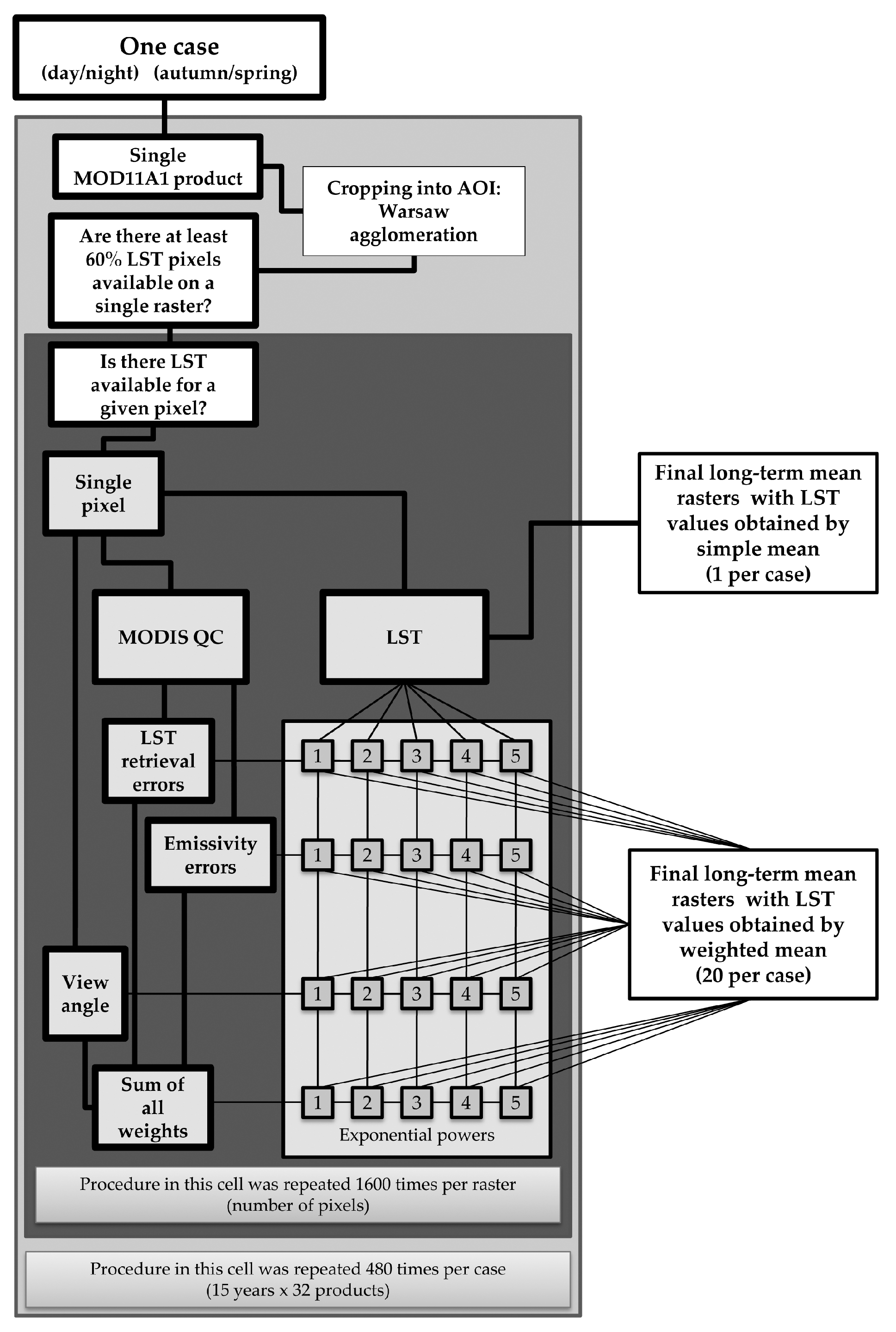
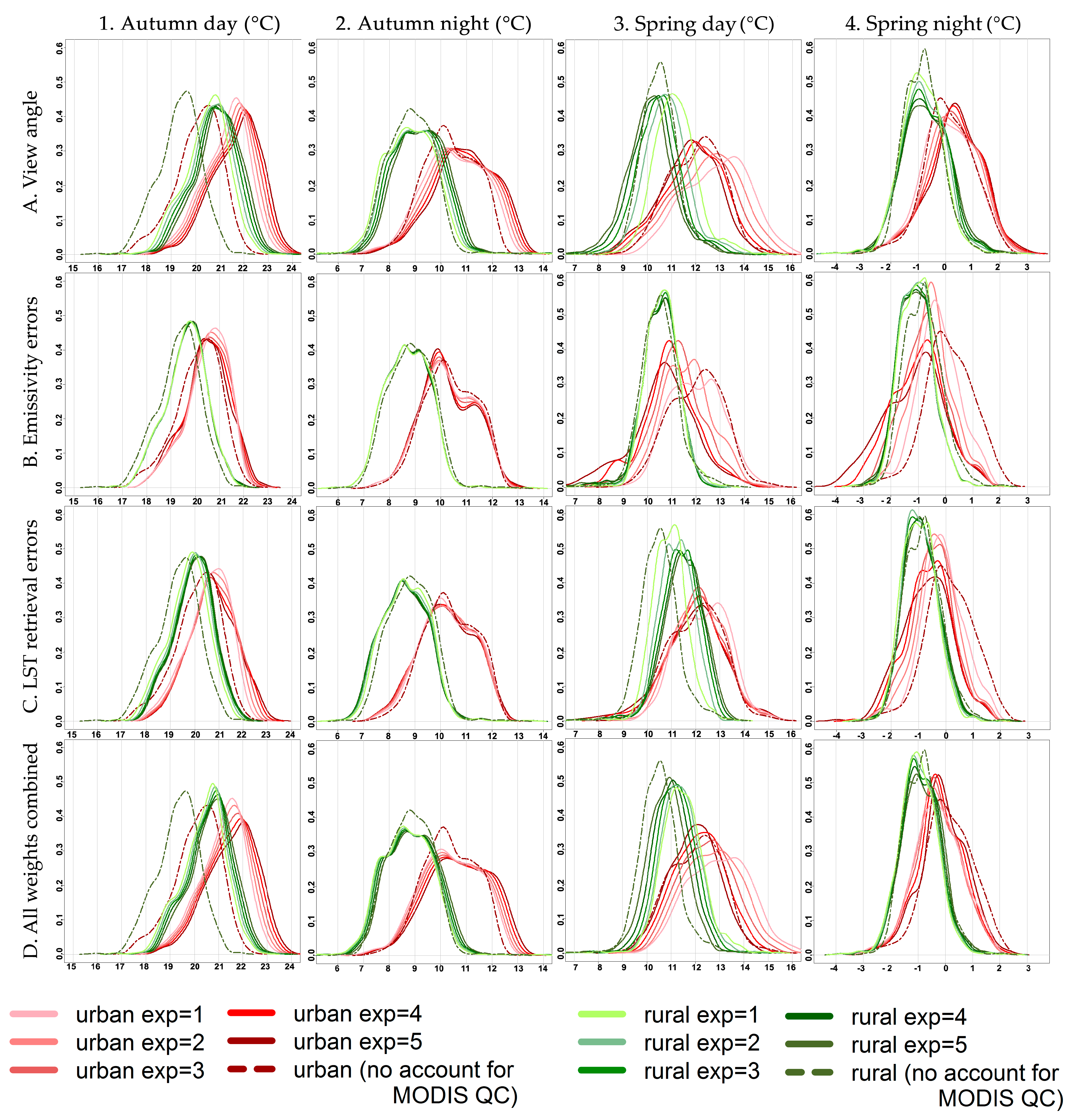
3.1. Density Distribution of Rural and Urban LST

In order to analyze differences between types of composition process, a set of PDFs of urban (red color) and rural (green color) LST was prepared (Figure 2). Urban pixels are referred to here as those that are located within the administrative boundaries of the city and rural areas are located outside the boundaries of the city, within the buffer zone (see Section 2 and Figure 3). PDF graphs were prepared for each raster constructed by means of the first (dotted lines) type of composition (without accounting for the MODIS QC). Solid lines represent rasters constructed with the second type of composition with five different exponential powers applied to weights during the aggregation process. To sum up, each pair of green lines and red lines represents a single raster.

Figure 2 shows differences in LST density between all types of raster constructed by different weights throughout different exponential powers. It is clear that temporal aggregation based on the second type of composition (weighted arithmetic mean) modifies all features of LST density distribution lines when compared with the first type of composition (simple mean); namely, maximum probability values, the range of expected LST, the slope of lines and the number of extremes. However, each type of composition in each season gives a different distribution of both urban and rural LST. Therefore, there is no general trend of influence by temporal aggregation with respect to the MODIS QC for LST distribution. Nevertheless, it must be underlined that, in each case, the distribution of rural LST is less diversified than the distribution of urban LST. This is true throughout each type of composition, exponential power, or season.

The lowest deviation between the first and the second type of composition is observed in autumn cases, especially in nighttime. In the autumn daytime case, the range of LST obtained by means of the first and second types of composition is similar, but there is a significant shift (about 1.5–2.5 °C) in minimum and maximum values of expected LST. In the autumn nighttime case, there is no significant shift in minimum and maximum LST. However, the range of LST is slightly wider (about 0.5–1 °C in 2A and 2D cells). In general, in autumn cases, the biggest impact on LST distribution is found on a view angle of satellite observation (row A). In most of the autumn cases, the lowest exponential power applied to weights gives urban LST distribution closest to that obtained by means of a simple arithmetic mean (cells 1A, 1D, 2A, 2B, 2C, and 2D).

Temporal aggregation with regard to the MODIS QC has a significant impact on LST distributions in spring cases. In both daytime and nighttime cases, the majority of density lines are not similar to each other, which proves that relevant differences exist between each threshold of best quality pixel promotion. In contrast to autumn cases, for most of the spring cases there is no clear answer to the question of whether exponential power makes LST distribution the closest to that obtained by the first type of temporal composition process. In most of the spring cases, there is no significant shift in expected maximum and minimum LST when two types of composition are compared (cells 3A, 3B and column 4). The highest shift is noted in cell 3C (of about 1–2 °C) and 4D (of about 1 °C), which is caused by weights based on LST retrieval errors.

There is no general answer to the question about which types of weight cause the biggest or lowest differences in LST distribution between the first and second types of composition or between exponential powers. However, weights based on view angle (Figure 2, row A) seem to give some systematic differences between LST distributions compared to weights based on emissivity errors (Figure 2, row B) or LST retrieval errors (Figure 2, row D).

When PDFs are compared with those documented by Gawuc [42] for summer cases, the conclusion is clear: the closest shapes in Figure 2 are those obtained for an autumn night. This is consistent with typical seasonal variability, since LST in summer is more similar to that during the autumn equinox than in the spring equinox.

3.2. LST Spatial Distribution Obtained by Means of Different Types of Weight

As the aim of the study was to estimate an average SUHI intensity for the last 15 years, it was critical to select an appropriate method to construct a temporal composite of mean LST. The combination of all types of weights (Figure 2, row D) gives the most reliable LST distribution when all exponential powers are considered. However, in order to prove that this type of weight is the most appropriate for further analyses, the spatial distribution of LST was investigated. The evaluation was performed visually with regard to previous studies of SUHI in Warsaw [39,40,41,42].

Figure 3 shows the 15-year mean LST spatial distribution for the area of Warsaw in the case of a spring day. Images were constructed by means of a weighted arithmetic mean, where weights were based on view angle (Figure 2, row A), emissivity errors (Figure 3, row B), LST retrieval errors (Figure 3, row C), and all of these combined (Figure 3, row D). Each type of weight had five degrees of exponential power applied (Figure 3, columns 1–3), which refers to the strength of the best quality pixel promotion. In addition, in Figure 3, we also present a 15-year mean LST pattern, which was constructed by means of a simple arithmetic mean, regardless of the MODIS QC metadata (named the first type of composition). According to synoptic conditions (e.g., snow occurrence, cloudiness) and consequent unavailability or low quality of remote sensing observations, the spring day case was the most difficult to estimate. Moreover, it gave the most diversified LST distribution, both in rural and urban areas (Figure 2, Section 3.1).

Figure 3 shows that each type of composition process with regard to the MODIS QC gives a different LST spatial pattern than a composition without regard to the MODIS QC. Rasters constructed by means of first exponential power have a clear pattern with elevated LST within the boundaries of the city. However, with growing exponential power, it becomes unclear (rows B and C), giving unrealistic LST patterns in urban areas. Nevertheless, images that are constructed by means of weights based on view angle and all weights combined (rows A and D) retain a typical urban LST pattern. The higher the exponential power applied, the lower the LST values obtained in the final images. Figure 2 and Figure 3 show that weight types A, B, and C are somehow compensating during a composition process involving type D weights.

To sum up, we chose combined weights for further analyses, since this type of temporal aggregation gave the most plausible shapes of PDFs and LST spatial distribution. Furthermore, it fully exploits the MODIS QC metadata.

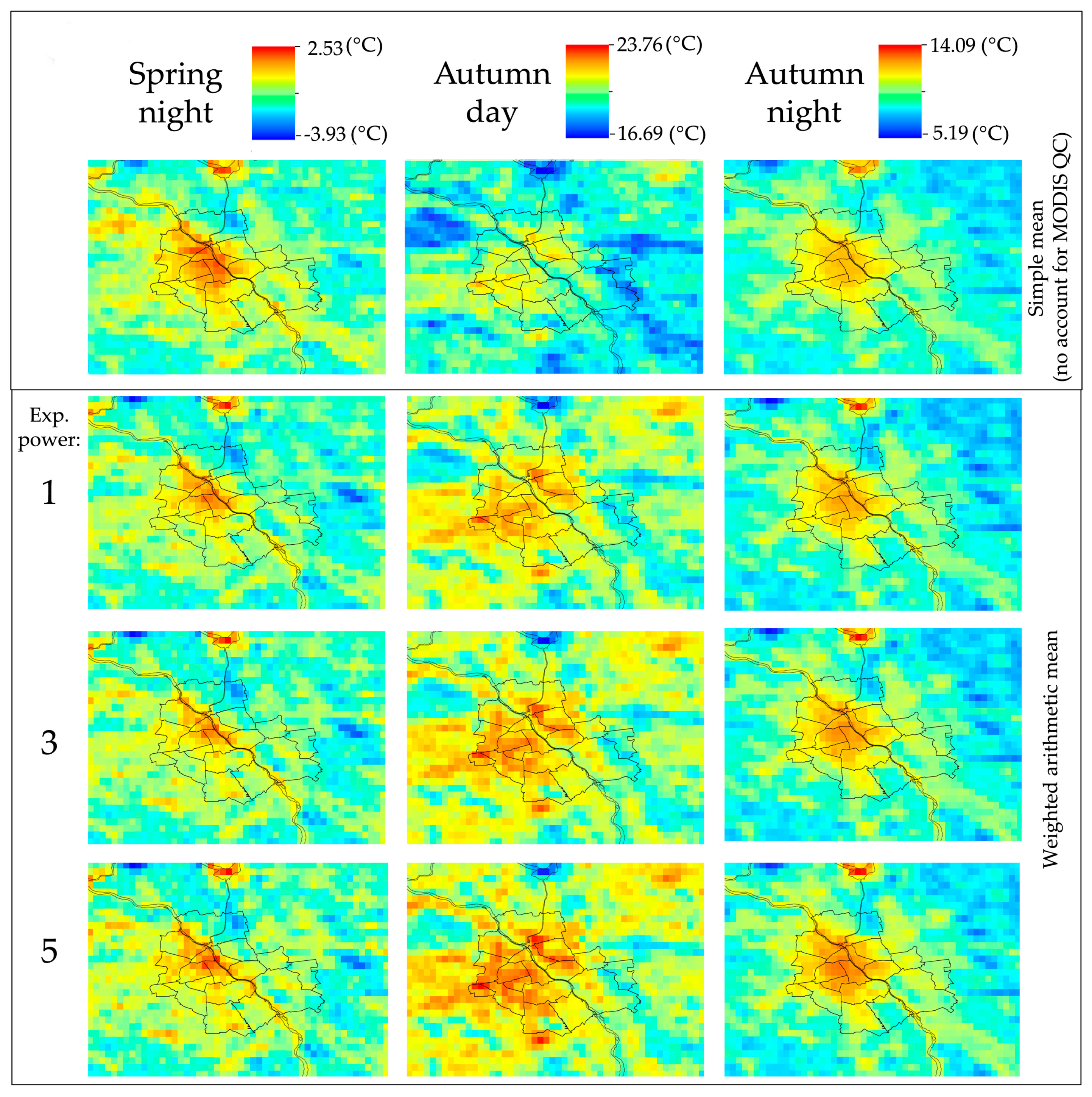
3.3. Spatial Distribution of LST in Different Seasons

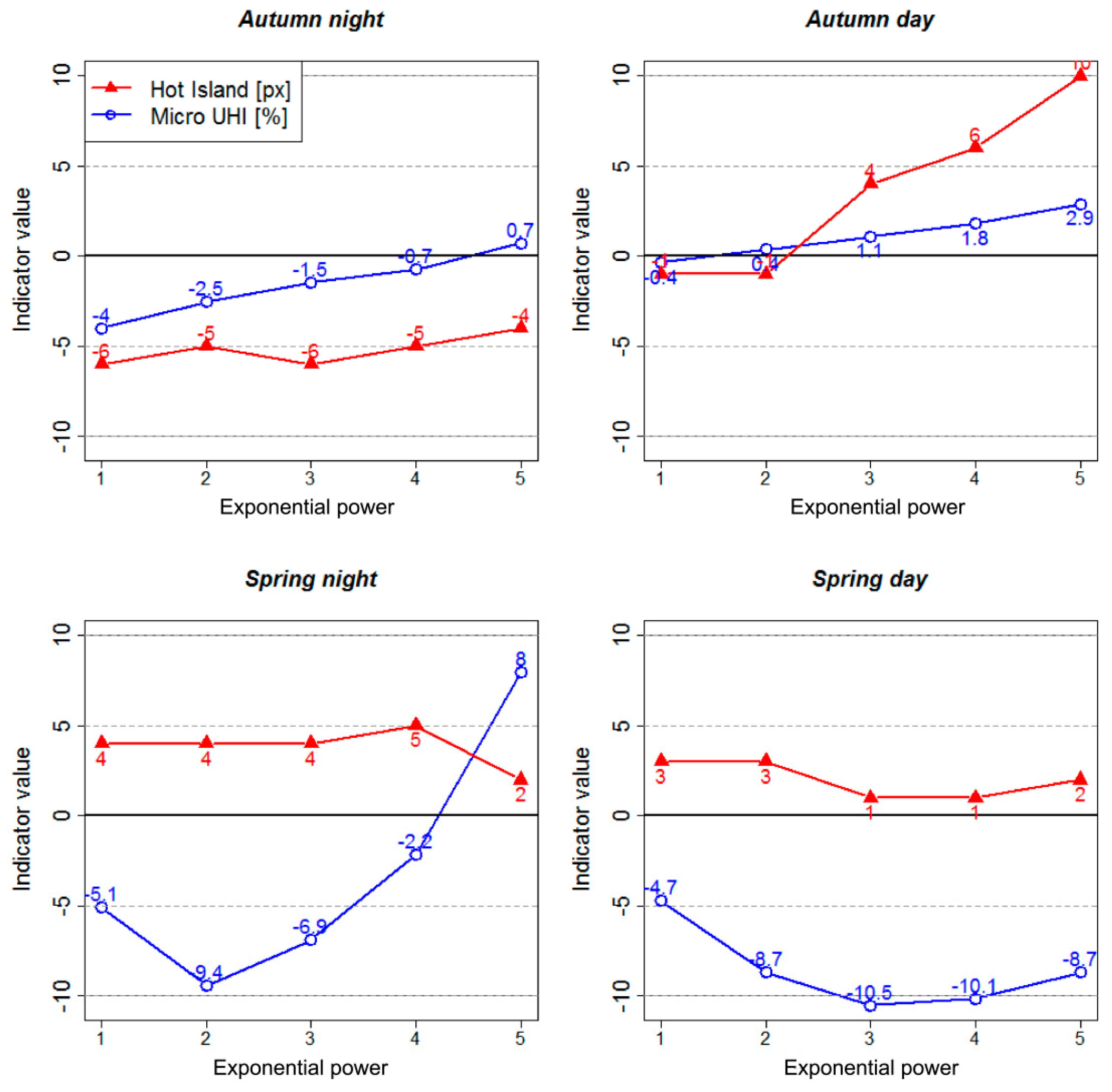
Figure 4 shows the spatial distribution of a 15-year mean LST obtained for each case: spring night, autumn day, and autumn night (the spring day case is presented in Figure 3, row D). Images were constructed using a sum of weights based on view angle, LST retrieval errors, and emissivity errors. Growing exponential power impacts the spatial range of elevated urban LST in spring cases—the bigger the exponential power, the smaller the spatial range.

On the other hand, growing exponential power does not result in a significant influence on the spatial range in autumn cases. However, it increases LST (Figure 2, Figure 3 and Figure 4). The daytime and nighttime cases show a different spatial pattern of LST (Figure 4). In the nighttime cases, the River Vistula is not visible in the middle of the city, but it is apparent outside the city’s borders. During daytime cases, the river is clearly visible in the urban area, but less visible outside the city’s borders. This is consistent with the typical diurnal variability of the LST pattern in Warsaw [39,40,41,42]. In each season, there are clear differences between rasters obtained by a simple mean and a weighed arithmetic mean; differences are especially visible in daytime cases, and less apparent in nighttime cases. Nevertheless, in each case, the LST pattern obtained by a weighted mean seems plausible.

3.4. SUHI Intensity

In order to underline the influence of the MODIS QC on a temporal composite of LST, we calculated SUHI indicator values on 15-year mean rasters, which were constructed by two types of arithmetic mean—simple (the first type of composition) and weighted (the second type of composition). The first type does not take into account the MODIS QC, while the second type does.

Table 3. Indicator values calculated on rasters that were constructed by means of a simple mean (first type of composition).

No	Indicator (°C)	Autumn Day	Autumn Night	Spring Day	Spring Night
1	Standard Deviation	0.92	1.00	1.10	1.10
2	Magnitude	2.16	1.89	3.21	2.52
3	Range	4.81	4.81	6.38	5.24
4	Urban mean—other	0.76	1.52	1.52	0.96
5	Urban mean—water	4.29	−2.05	6.57	−1.92
6	Urban mean—agriculture	−0.04	1.40	2.29	0.85
7	Inside urban—inside rural	1.12	1.34	1.42	1.02
8	Urban core—rural ring	1.04	2.26	1.84	1.4
9	Urban core—deep forest	3.08	1.32	3.52	0.05
10	Hot island (pixels)	45	67	51	45
11	Micro-UHI (%)	88.33	50.00	73.19	30.07

shows the SUHI indicator values calculated on rasters that were constructed by means of a simple mean. Figure 5 and Figure 6 shows the differences between values of indicators as a result of subtraction: A indicator calculated by the second type of composition minus the same indicator calculated by the first type of composition.

It is clear that, in each season analyzed, the SUHI phenomenon does occur (Table 3). The strongest SUHI is noted on a spring day. However, it is unclear since not all of the indicators have the highest values in this case (“8,” “10,” “11”). Moreover, it is hard to judge in which season the SUHI intensity is the lowest, since the behavior of indicators is inconsistent. Several indicators have the lowest values for the spring night (numbered “6,” “7,” “9,” and “11”), while other indicators have the lowest values for the autumn day (“1,” “4,” “6,” and “8”). The smallest SUHI compared to others was for the “urban mean—other” indicator, while the highest was for “urban mean—water” and “range.” The indicators “range” and “urban mean—other” can be compared with [42]. As reported, the “range” may reach 6.3 °C on the summer night, which is similar to the spring day case here. “Urban mean—other” was almost the same in the summer case in relation to a single MODIS observation in the day (2.2 °C) and night (2.1 °C). Here, we report its diurnal variation, with lower values in the autumn day and the spring night, while there are higher values in the autumn night and the spring day. Utilizing the “magnitude” indicator, [63] reported smaller daytime SUHI than in the nighttime. Here, results are opposite: stronger SUHI is noted in the daytime and weaker in the nighttime in both analyzed seasons. In [57], “urban mean—agriculture” revealed a small variability range across the measurements and points in time. Here, we note that other indicators have smaller seasonal and diurnal variability. We also observed a very slight SUHS [5]. In [64], the indicator “inside urban—inside rural” is higher at night than during the day. Here, we report that this is consistent with the autumn case and inconsistent with the spring case. However, diurnal changes are quite small. “Urban core—deep forest” has not yet been used in the literature. It emphasizes the daytime SUHI magnitude, especially in the spring case. In [57], the indicator “urban core—rural ring” revealed a smaller SUHI with a lower diurnal change; meanwhile, in [65], this indicator showed higher values for daytime. This is consistent with the spring case and inconsistent with the autumn case.

In most of the cases (except the spring night case and the “urban mean—water” indicator in the spring day case), there is a clear trend—the higher the exponential power applied to weights, the bigger the difference between two types of composition (Figure 5). This corresponds to the strength of best quality pixel promotion. The indicator “urban mean—water” reveals a notable inversion of SUHI in nighttime cases—SUHS [5]. In the daytime spring case, it had a higher value than any other indicator calculated. Given that the diurnal variation of surface water temperature is small, it reveals a strong diurnal change in LST in the urban area. The variation of “urban mean—water” is highest in the spring day.

The indicator “magnitude” is quite stable though exponential powers, apart from an exception for the spring day case, while “range,” which is calculated by pixels with extreme values, is unstable though exponential powers. In the spring night case, the indicators’ behavior is as follows: rising exponential power from first to second lowers its values; from second to third, power indicators are stable; and from third to fifth, indicator values are rising. However, the indicator “range” is rising from the second to the fifth exponential power, while “urban core—deep forest” is dropping from the first to the fifth exponential power. It is also much more stable for exponential powers in nighttime cases.

For the autumn case, almost every indicator calculated with the help of the first type of composition is the same or only slightly higher than indicator calculated with the help of the second type of composition. This means that growing exponential power applied to weights during the composition process causes higher contrasts in LST observable in urban and rural areas and directly increases SUHI intensity. Nevertheless, the differences between two types of composition are very low—lower than 0.5 °C. Two exceptions are the indicator “urban mean—agriculture” in the autumn night case and “urban core—deep forest” in the autumn day case. “Urban mean—agriculture” is stable in autumn cases for exponential powers and quite unstable in spring cases. Each indicator in the spring night case, calculated by means of the second type of composition, has a lower value than after processing with the first type. In the spring day case, the indicator “urban mean—agriculture,” calculated by means of the second type of composition, has higher values than after processing with the first type of composition. All other indicators in the spring day case, starting with the third exponential power, are lower when calculated by means of a raster processed with the second type of temporal composition process rather than with the first type. Since “hot island” and “micro-UHI” indicators have different units and higher values, they are presented separately (Figure 6).

It is observable that the highest differences between two types of temporal composition processes are observed in spring cases, corresponding to the high variability of synoptic conditions throughout the 15-year period in this season and the consequent low quality of satellite observations. “Hot island” and “micro-UHI” indicators are expressed in units of area and reveal different variability with exponential powers (Figure 6). Depending on the case, growing exponential power may increase, decrease, or have no impact on SUHI intensity. Moreover, in specific cases, the trend may be inverted from decreasing to increasing with growing exponential power (spring cases only). The hot island shows a rather strong stability through exponential powers, but only in spring cases. The lowest differences between two types of composition process are noted in the autumn day case for the “micro-UHI” indicator and in the spring day for the “hot island.” However, it is clearly not apparent in which season—spring or autumn—the impact of the inclusion of the MODIS QC metadata in the temporal aggregation process on SUHI intensity is higher. “Micro-UHI” reveals a clearly growing trend in autumn cases with growing exponential powers. However, it is very unstable in the spring night case and quite unstable in the spring day case. As previously reported by [18,57], the “micro-UHI” and “hot island” were larger for the night than for the day. Here, the behavior of the “micro-UHI” is inverted, while the “hot island” gave smaller or higher SUHI with no consistency.

In summary, an analysis of Table 3 and Figure 5 and Figure 6 leads to the conclusion that a temporal composition process with regards to the MODIS QC has a clear impact on the calculated intensity of SUHI phenomena. In autumn cases, it mostly increases, while it decreases SUHI intensity in spring cases. However, some of the indicators show a different relationship with temporal aggregation processes and with the strength of best quality pixel promotion. The indicators, which are referred to as area units, show different behaviors than those indicators expressed in Celsius.

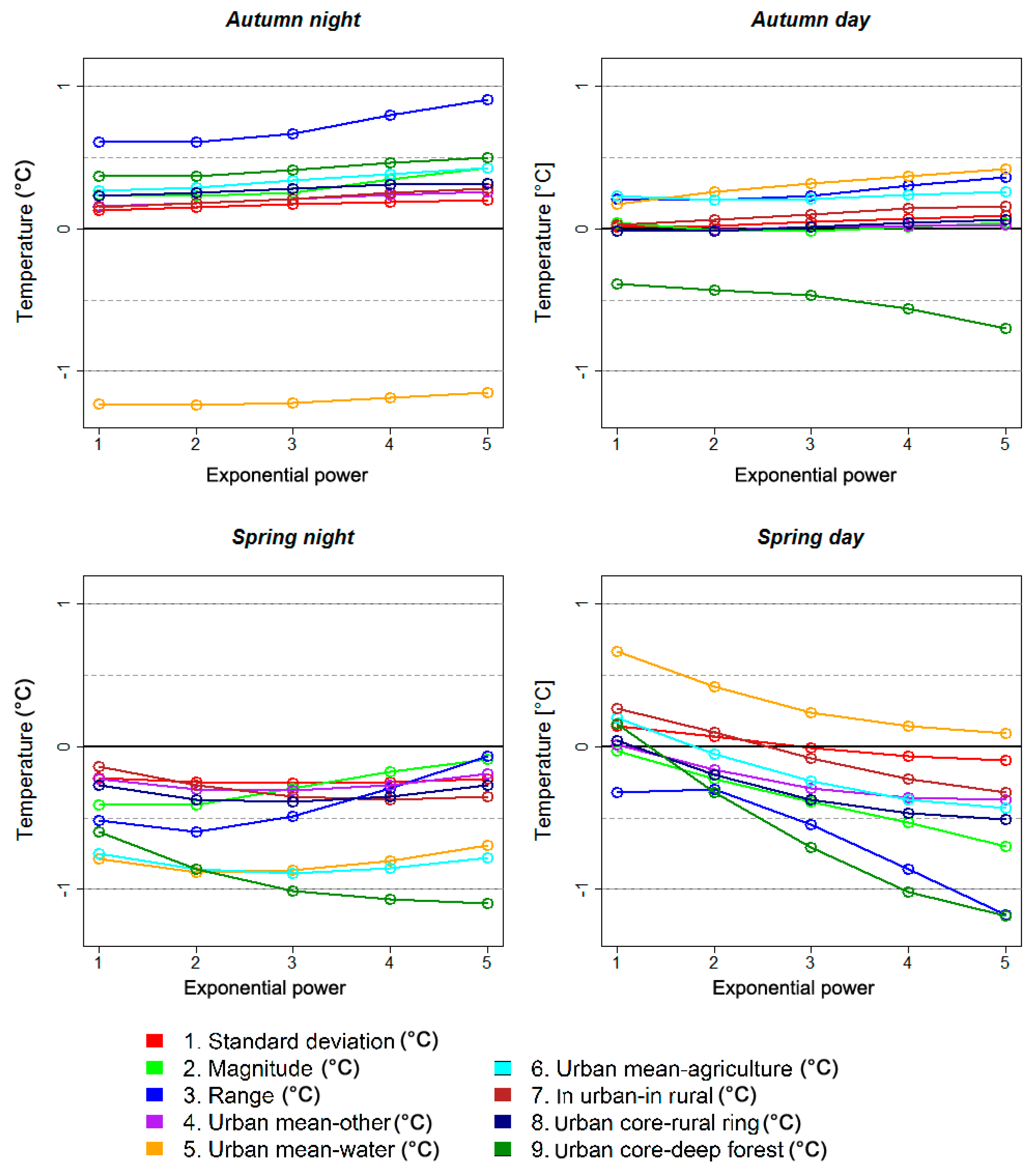
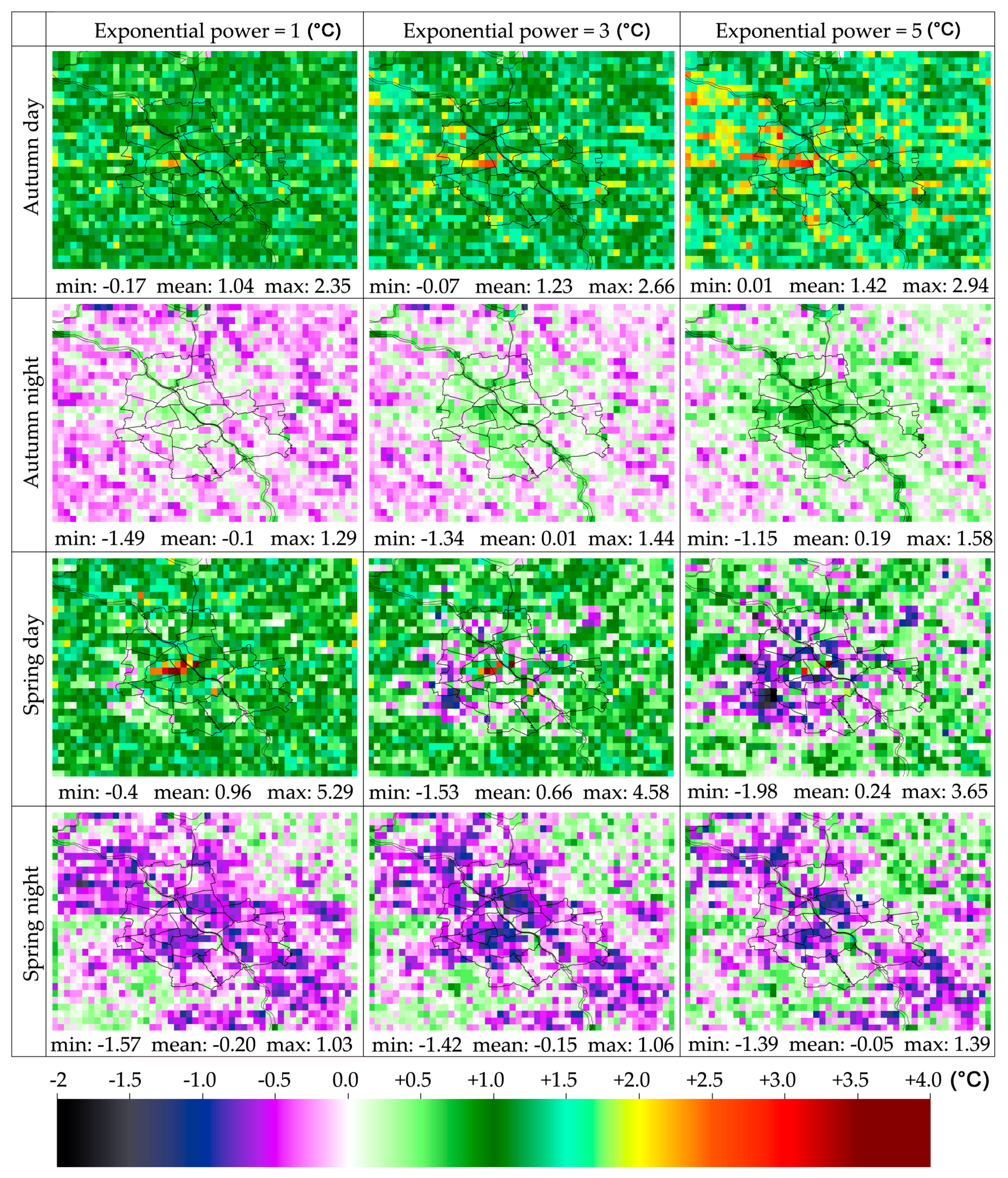
3.5. Comparison of the Impact of the First and Second Types of Temporal Composition on the Spatial Pattern of LST—A Differential Approach

In Section 3.4., we discussed differences between SUHI intensities calculated on rasters obtained by means of a simple (the first type of composition) and a weighted arithmetic mean (the second type of composition). However, such an analysis does not reveal the impact of the second type of composition on the final spatial pattern of LST. To fill this gap, we prepared a set of differential maps showing pixel values as a result of subtraction: a 15-year mean raster built by the second type of composition minus a 15-year mean raster built by the first type of composition process (Figure 7). In order to maintain brevity in this paper, differential rasters with two and four exponential powers are not presented.

In each season, the behavior of differences throughout exponential powers is different (Figure 7). In autumn cases, the mean value of differences is increased with growing exponential power, while it is decreased in spring cases. In the autumn day case, almost all of the pixels have a positive sign, whereas low exponent values are about 1–1.5 °C. With growing exponential power, differences are increased by up to 2.94 °C. The highest differences are observed in the very center of the city and in northwestern rural areas.

In the autumn night case, most of the values are lower (approximately between −0.5 and −1 °C with a low exponent and about 1 °C with a high exponent) than in the autumn day case; meanwhile, most of the differential pixels in rural areas have a negative sign, but a positive sign in urban areas. Moreover, growing exponential power not only changes the magnitude of differences but also their sign. A low exponent indicates many negative differences, while a high exponent indicates fewer negative and more positive differences in rural areas, as well as increased values of differential pixels in urban areas due to a high exponent. The autumn night case is the only one case in Figure 7 where there is a clear pattern of pixels associated with the River Vistula.

When the low exponent is applied, the majority of differential pixels in the spring day case indicate a positive sign, along with magnitudes from about 0.5 °C to 1.5 °C. However, some pixels have a negative sign and a value of about −0.5 °C. In addition, there are pixels with very high values exceeding 5 °C. Growing exponential power profoundly changes pixels values. The majority of the pixels located in the most distant rural areas away from the city boundaries—in the western and southern parts of the image—retain their positive sign, while their values are not significantly modified by a growing exponent. However, some pixels located in the northern and eastern parts of rural areas have both their sign and magnitude modified (from about 1–1.5 °C to −1 °C). The most distinctive changes have a place in urban areas and locations close to the city’s administrative boundaries, where most of the pixels change their sign and values from a positive of about 1–1.5 °C to a negative approximately between −1 and −1.5 °C. Moreover, on the western border, there are several pixels with the lowest differential values in any case, which are observed reaching almost 2 °C; also at this location, when different exponential powers are applied, there are significant changes in value observed—from a positive of about 1 °C to a negative of about −1 °C. In the very center of the urban areas, there are several pixels with the highest positive values observed in any case. However, their values are lowered as exponential power is increased.

In the spring night case, the majority of differential pixels have values close to zero or approximately between −0.1 and −1 °C, the exception being in the southwestern and northeastern parts of the image. Such a differential pattern is mostly retained with growing exponential power. However, some pixels change their sign from negative to positive or the reverse. Furthermore, the magnitudes of difference are modified. Similar to other cases, the highest differences are mostly located in the urban area. When the highest exponent is applied, there are two “hot spots” visible in an urban area with negative differential values approximately between −1.3 and −1 °C.

Figure 7 shows the actual location and magnitude of differences in LST between the first and the second type of composition. Since the highest differences are observed within the administrative borders of the city, it is important to investigate the percentage by which urban areas are covered with pixels of relevant differential values.

Table 4. Percentage of urban areas covered with growing differential thresholds.

Season	Exponential Power	>0.5 °C	>1.0 °C	>1.5 °C	>2.0 °C	>2.5 °C	>3.0 °C
Autumn day	1	98%	46%	11%	2%	0%	0%
	2	98%	58%	16%	3%	0%	0%
	3	99%	70%	21%	4%	1%	1%
	4	99%	81%	34%	7%	1%	1%
	5	99%	70%	21%	4%	1%	1%
Autumn night	1	2%	0%	0%	0%	0%	0%
	2	6%	0%	0%	0%	0%	0%
	3	13%	0%	0%	0%	0%	0%
	4	25%	0%	0%	0%	0%	0%
	5	37%	2%	0%	0%	0%	0%
Spring day	1	82%	42	13%	5%	2%	2%
	2	62%	28%	7%	2%	2%	2%
	3	50%	15%	5%	2%	1%	1%
	4	43%	9%	2%	1%	1%	1%
	5	42%	11%	2%	1%	1%	1%
Spring night	1	37%	2%	0%	0%	0%	0%
	2	42%	8%	0%	0%	0%	0%
	3	41%	9%	0%	0%	0%	0%
	4	33%	7%	0%	0%	0%	0%
	5	29%	5%	0%	0%	0%	0%

shows the percentage of urban area covered with growing thresholds of difference.

When high exponential power is applied, a significant part of the urban area is covered with high differential values (Table 4). Moreover, in the spring day case, about 2% of urban areas are covered with differences higher than 2.5 °C and 3.0 °C when exponents 1 and 2 are applied; where exponents 3 to 5 are applied, the percentage of areas with high differences is decreased. It is clear that, in the nighttime cases, the percentage of areas with differences higher than 1 °C is very low. However, in the daytime cases, a very significant area of the urban area is associated with differences higher than 2 °C. To sum up, a significant part of the urban area is covered with differences between the first and second types of temporal composition higher than 0.5–1 °C in nighttime cases and higher than 1.5–2 °C in daytime cases.

4. Discussion

In spite of the fact that the presented methodology clearly documents the impact of the MODIS QC and the view angle on temporal composites of urban LST, there are several comments that are necessary.

4.1. The Representativeness of Satellite Remote Sensing Data in Terms of MODIS Observations

It is obvious that remote sensing observations are influenced by many factors, which inevitably limits their applicability. Roy et al. [66] gives a comprehensive review of the quality assessment approach to MODIS land products and lists more than 10 possible sources of errors. Fourteen years later, some of these have been improved with the introduction of new data collection methods, for example, the cloud screening issue; however, as the Terra satellite gets older, the frequency of malfunctions may increase. Taking into consideration poor atmospheric conditions, there is generally a great deal of missing information, which reduces usage rate and hinders the follow-up interpretation. Therefore, a number of missing information reconstruction techniques have been developed [67]. Utilizing multi-sensor fusion methods would be an interesting way to obtain the most representative fine scale long-term urban LST composites [68,69]. However, we focused on a single sensor to present the impact of including the quality metadata in the temporal aggregation process. We utilized all available information about the quality of MODIS observations. Thus, we assumed that the obtained results are representative. Nevertheless, to objectively judge whether our methodology gives the most realistic temporal composites, a more comprehensive evaluation would be needed. However, this would require obtaining ancillary (in situ and/or airborne) data, which, given that the obtained results are consistent with previous studies, exceeds the scope and aims of the paper.

Data quality is a critical issue for a reliable long-term time series [70]. The MODIS QC is known for inconsistencies in quality flags [62], which may cause abnormal QC flag distribution. This is mostly due to the nature of the split-window algorithm, which underestimates cloud contamination [71]. The MODIS QC flags are specified by an automated algorithm during the calculation of the satellite product. The MODIS cloud masking philosophy flags a pixel as cloudy where at least one of the spectral tests detects a cloud with a high confidence level. This is known as the “clear sky conservative” approach, as the goal is to minimize the misclassification of cloud-free pixels as cloudy. However, this creates a risk that some cloud-free pixels will be incorrectly classified as cloudy [72]. According to the nature of satellite remote sensing observations, it may be presumed that the lowest errors of LST retrieval might be indicated during specific synoptic conditions—for example, when very strong wind dilutes atmospheric aerosols, which results in enhanced visibility. This would mean that “the best quality” term, as used in the presented study, may not give the most representative image of urban LST, while detailed analysis of synoptic conditions resulting in an appropriate adjustment of quality weights would be needed. However, this would have to be done for each moment of satellite observation, which again exceeds the scope of this paper.

4.2. Findings of This Study in Light of Previous Studies of SUHI in Warsaw

Previous studies of SUHI in Warsaw are very scarce. To date, there are three studies that utilized Landsat TM data, one that utilized AVHRR, and two that utilized MODIS data. None of them used temporal composites. However, these studies were used as a generalized clue to evaluate the obtained spatial distributions by means of different weights applied in the temporal composition process. We chose a temporal composition that takes into account all available information about the quality of MODIS observations.

In our study, we found that the impact of MODIS QC and view angle on long-term LST composites is weaker in the nighttime cases than in the daytime cases. This is consistent with remarks made in [73], where the authors conclude that the “nighttime differences are far less influenced by the viewing geometry, and result from a wide range of factors, such as (1) the use of different land surface emissivity maps; (2) calibration uncertainties of each sensor; and (3) calibration uncertainties of the parameters in the respective split window algorithms.”

4.3. SUHI Indicators

Schwarz et al. [57] documented weak correlations between SUHI indicators. Here, the utilized SUHI indicators show different behavior when gradual exponential powers are applied. In each analyzed case, there is a group of indicators that reveals very similar behavior, while other indicators stand out. However, in each case, this group consists of different indicators. Therefore, our findings are consistent with [57].

As reported in [57], for most of the indicators, the SUHI was highest in the daytime. Here, the same conclusion can be made. Smaller values are noted for those indicators that utilize a larger amount of pixels (“urban mean—other” and “urban core—rural ring”); analogically, a higher SUHI is noted for indicators that are referred to specific single pixels (“range” and “magnitude”). Schwarz et al. [18] question the usage of single values for the UHI for a whole city because of the explanatory power of such an indicator. It may be stated that this is particularly true when sensors with high spatial resolution are utilized. However, they might be useful for analyses of air UHIs measured by sparse in situ networks.

Analysis of SUHI intensities, in terms of their variability with growing exponential power applied to weights during the composition process (Section 3.4), as well as the PDF of LST in urban and rural areas (Section 3.1), shows that the SUHI phenomenon occurs in each analyzed case. However, it is observable that the behavior of SUHI indicators varies. Furthermore, there is no clear answer as to which indicator is the most independent from growing exponential power applied to weights during the composition process. Thus, in spite of the certainty that the SUHI phenomenon does occur in the city of Warsaw in each analyzed case, it is hard to draw any conclusions about its 15-year mean intensity. However, it might be stated that the mean SUHI magnitude has at least 1 °C in each analyzed season and, in specific cases, might be much higher.

4.4. The Amount of Data Utilized

It is found that the long-term mean LST, aggregated with an account for MODIS QC, significantly differs from temporal aggregation without an account for MODIS QC metadata. However, in this study, the actual impact of MODIS QC on final LST patterns is increased by the long period of weight accumulation (15 years), resulting in the number of the rasters utilized (at least 174). Studies devoted to shorter periods with fewer data included indicated that such an impact might be less apparent. However, as stated in [66], in many cases, issues that affect product performance are only seen in the examination of a long-term product series or by examination of temporally composited products.

In most of the cases analyzed, the highest impact of temporal aggregation with an account for MODIS QC is revealed when high exponential power is applied to weights during the composition process. However, this study does not give a clear answer as to what constitutes a proper exponential power that ought to be applied to weights in similar studies. According to the specifics of the construction of urban areas and natural uncertainties associated with thermal satellite observations, it seems important to aim for the most accurate LST estimation in every investigation (thereby promoting pixels with the highest quality). Meanwhile, the appropriate strength of the promotion is unknown. In general, it must be concluded that the choice must depend on a specific case; for example, when fewer data (than in this study) are taken into account, higher exponential powers may be used.

4.5. The Location of the Most Profound Impact of MODIS QC on a Long-Term LST Composite

Table 4 shows the percentage of the city associated with high differences between two types of temporal composition. It is important to comment that 1% of areas covered with differences higher than 3 °C should not be neglected (daytime cases). The MODIS pixel covers 1 km² in the nadir view on the equator; however, according to the curvature of the Earth, with regard to Warsaw’s longitude of 52°, the area covered with MODIS pixels is bigger. Taking into account the number of level 3 pixels within the administrative borders of Warsaw (321), 1% refers to more than 3.21 km² of the urban area. According to the findings of this paper, in which the highest impact of MODIS QC on the results of temporal aggregation is typically observed in the city center, it becomes clear that 1% of the urban area with the highest differences is located in the very center of the city. As reported by [74], this refers to the same area where the most profound effect of air UHI in Warsaw is observable.

4.6. The Emphasis of the View Angle in Temporal Composition

Since LST retrieval errors and emissivity errors have five thresholds described according to the MODIS Collection 5 User Guide [58], there were also five weights based on the magnitude of errors in this study. However, weights based on the view angle of satellite observation had nine thresholds specified (Table 1). This creates inequality in the impact of the weights on the final results, especially when high exponential powers are applied. However, thermal anisotropy is a factor that can influence temperature retrieval and, therefore, thermal time series [75]. Hence, numerous researchers conclude that accounting for angular dependencies is critical. The experimental data showed that the differences between nadir and off-nadir values of directional temperature are of considerable magnitude and, as such, cannot be ignored [76]. Angular correction of satellite retrieved LST must be applied before LST data can be compiled into a long-term data set, assimilated into weather prediction models or used in climate research [77]. The accuracy of MODIS products may be affected by errors in land surface emissivity. While the errors that occur in MODIS LST products are weakly, but they are, view angle dependent [78]. The IFOV grows considerably for off-nadir observations, especially in the across-track direction. Therefore, the cases for which the MODIS viewing angle is larger than 40° should be considered with care, since they may be affected by larger uncertainties [61].

According to the remarks given above and inconsistencies in MODIS QC flags (see Section 2.2), along with the fact that the specification of the view angle in MODIS products is faultless, inequality in the impact of different types of weights on the final results seems legitimated.

4.7. Applicability of Presented Methodology to Similar Studies

Each type of weight gave different density distribution and spatial distribution of LST (Section 3.1 and Section 3.2). Rasters constructed by means of MODIS data quality flags (LST retrieval errors and emissivity errors) gave an unrealistic pattern of urban LST, which leads to the conclusion that temporal aggregation based solely on such metadata may result in significant discrepancies. When weights based on the view angle are also included in the composition process, the image obtained by means of all types of weight combined gives a plausible urban LST pattern.

The overall differential spatial pattern of LST obtained by the first and second types of temporal composition process is highly diversified (Figure 7). It is quite common for adjacent urban pixels to have very different values or even opposite signs, or that growing exponential power changes the increasing or decreasing trend of differences. This underlines the importance of MODIS QC for long-term urban LST monitoring. Hence, it is concluded that a weighted arithmetic mean, which fully exploits MODIS QC metadata and the view angle of observations, might be an appropriate tool to construct a temporal composite of urban LST. It could be suggested that, in studies focused on other cities with more high-rise buildings in the city center, the impact of MODIS QC on temporal composites might be higher than in the presented study. However, given that no field validation was applied, additional studies are required to analyze and validate the proposed methodology with other approaches.

Since the weights applied during the composition process were explicitly based on quality thresholds and the view angle indicated by MOD11A1 QC, the applicability of the presented methodology for other satellite instruments is limited to those products that contain appropriate metadata, such as products available from AATSR [79], VIIRS [80], and SEVIRI [81], or the recently launched Sentinel-3 [82].

5. Conclusions

The goal of the presented study was to estimate a mean SUHI intensity for Warsaw, a Central European agglomeration, in transitional seasons (spring and autumn) by obtaining the most representative LST image for a 15-year period. The intention behind the approach was based on an assumption that, according to the nature of thermal remote sensing observations and typical synoptic conditions over the study area, it is justified to put an emphasis on high-quality pixels. Therefore, a weighted arithmetic mean was applied in order to calculate the final rasters that represent the mean LST values for the period from 2000 to 2014. Weights were accumulated over 15 years and based on MOD11A1 QC metadata (LST retrieval errors and emissivity errors) and view angles.

The most important conclusion is that, accounting for the MODIS QC and the view angle of satellite observation in the temporal aggregation process was found to have a significant impact on the long-term urban LST composites. Analysis of temporarily aggregated LST for each analyzed case (Section 3.1, Section 3.2, Section 3.3, and Section 3.5) shows that the temporal aggregation process has a clear impact on the values, the spatial pattern of urban and rural LST, and the density distribution of both urban and rural LST. This remark is consistent with the findings of [6]. However, the impact of MODIS QC and the view angle on long-term SUHI intensity is less distinctive than on an LST spatial pattern (Section 3.4).

The impact of the MODIS QC and the view angle on temporal composites is more distinct during spring cases than autumn cases, as well as more distinct during daytime cases than nighttime cases. This is consistent with a higher variability of synoptic conditions in spring cases and the daytime, alongside the lower impact that thermal anisotropy has on nighttime thermal imagery. It is also acknowledged that the most profound effect of MODIS QC was observed in the city center.

References

1. Oke, T.R. The Heat Island of the Urban Boundary Layer: Characteristics, Causes and Effects. In Wind Climate in Cities; Cermak, J.E., Davenport, A.G., Plate, E.J., Viegas, D.X., Eds.; NATO ASI Series; Springer: Dordrecht, The Netherlands, 1995; pp. 81–107. [Google Scholar]
2. Sahin, M. Modelling of air temperature using remote sensing and artificial neural network in Turkey. Adv. Space Res. 2012, 50, 973–985. [Google Scholar] [CrossRef]
3. Voogt, J.A.; Oke, T.R. Thermal remote sensing of urban climates. Remote Sens. Environ. 2003, 86, 370–384. [Google Scholar] [CrossRef]
4. Roth, M.; Oke, T.R.; Emery, W.J. Satellite-derived urban heat islands from three coastal cities and the utilization of such data in urban climatology. Int. J. Remote Sens. 1989, 10, 1699–1720. [Google Scholar] [CrossRef]
5. Clinton, N.; Gong, P. MODIS detected surface urban heat islands and sinks: Global locations and controls. Remote Sens. Environ. 2013, 134, 294–304. [Google Scholar] [CrossRef]
6. Hu, L.; Brunsell, N.A. The impact of temporal aggregation of land surface temperature data for surface urban heat island (SUHI) monitoring. Remote Sens. Environ. 2013, 134, 162–174. [Google Scholar] [CrossRef]
7. Stewart, I.D.; Oke, T.R. Local Climate Zones for Urban Temperature Studies. Bull. Am. Met. Soc. 2012, 93, 1879–1900. [Google Scholar] [CrossRef]
8. Mallick, J.; Rahman, A.; Singh, C.K. Modeling urban heat islands in heterogeneous land surface and its correlation with impervious surface area by using night-time ASTER satellite data in highly urbanizing city, Delhi-India. Adv. Space Res. 2013, 52, 639–655. [Google Scholar] [CrossRef]
9. Stroppiana, D. Seasonality of MODIS LST over Southern Italy and correlation with land cover, topography and solar radiation. Eur. J. Remote Sens. 2014, 47, 133–152. [Google Scholar] [CrossRef]
10. Goïta, K.; Royer, A.; Bussières, N. Characterization of land surface thermal structure from NOAA-AVHRR data over a northern ecosystem. Remote Sens. Environ. 1997, 60, 282–298. [Google Scholar] [CrossRef]
11. Stathopoulou, M.; Cartalis, C. Daytime urban heat islands from Landsat ETM+ and Corine land cover data: An application to major cities in Greece. Sol. Energy 2007, 81, 358–368. [Google Scholar] [CrossRef]
12. Amiri, R.; Weng, Q.; Alimohammadi, A.; Alavipanah, S.K. Spatial-temporal dynamics of land surface temperature in relation to fractional vegetation cover and land use/cover in the Tabriz urban area, Iran. Remote Sens. Environ. 2009, 113, 2606–2617. [Google Scholar] [CrossRef]
13. Kant, Y.; Bharath, B.D.; Mallick, J.; Atzberger, C.; Kerle, N. Satellite-based analysis of the role of land use/land cover and vegetation density on surface temperature regime of Delhi, India. J. Ind. Soc. Remote Sens. 2009, 37, 201–214. [Google Scholar] [CrossRef]
14. Sun, Q.; Wu, Z.; Tan, J. The relationship between land surface temperature and land use/land cover in Guangzhou, China. Environ. Earth Sci. 2011, 65, 1687–1694. [Google Scholar] [CrossRef]
15. Walawender, J.P.; Szymanowski, M.; Hajto, M.J.; Bokwa, A. Land Surface Temperature Patterns in the Urban Agglomeration of Krakow (Poland) Derived from Landsat-7/ETM+ Data. Pure Appl. Geophys. 2014, 171, 913–940. [Google Scholar] [CrossRef]
16. Frey, C.M.; Kuenzer, C.; Dech, S. Cross-Comparison of Daily Land Surface Temperature Products from NOAA-AVHRR and MODIS. In Thermal Infrared Remote Sensing: Sensors, Methods, Applications; Remote Sensing and Digital Image Processing; Springer: Dordrecht, The Netherlands, 2013; Volume 17, pp. 215–232. [Google Scholar]
17. Nichol, J.E.; Fung, W.Y.; Lam, K.; Wong, M.S. Urban heat island diagnosis using ASTER satellite images and “in situ” air temperature. Atmos. Res. 2009, 94, 276–284. [Google Scholar] [CrossRef]
18. Schwarz, N.; Schlink, U.; Franck, U.; Großmann, K. Relationship of land surface and air temperatures and its implications for quantifying urban heat island indicators—An application for the city of Leipzig (Germany). Ecol. Indic. 2012, 18, 693–704. [Google Scholar] [CrossRef]
19. Azevedo, J.A.; Chapman, L.; Muller, C.L. Quantifying the Daytime and Night-Time Urban Heat Island in Birmingham, UK: A Comparison of Satellite Derived Land Surface Temperature and High Resolution Air Temperature Observations. Remote Sens. 2016, 8, 153. [Google Scholar] [CrossRef]
20. Ho, H.C.; Knudby, A.; Xu, Y.; Hodul, M.; Aminipouri, M. A comparison of urban heat islands mapped using skin temperature, air temperature, and apparent temperature (Humidex), for the greater Vancouver area. Sci. Total Environ. 2016, 544, 929–938. [Google Scholar] [CrossRef] [PubMed]
21. Dousset, B.; Gourmelon, F. Satellite multi-sensor data analysis of urban surface temperatures and landcover. ISPRS J. Photogramm. Remote Sens. 2003, 58, 43–54. [Google Scholar] [CrossRef]
22. Yuan, F.; Bauer, M.E. Comparison of impervious surface area and normalized difference vegetation index as indicators of surface urban heat island effects in Landsat imagery. Remote Sens. Environ. 2007, 106, 375–386. [Google Scholar] [CrossRef]
23. Xiao, R.; Ouyang, Z.; Zheng, H.; Li, W.; Schienke, E.W.; Wang, X. Spatial pattern of impervious surfaces and their impacts on land surface temperature in Beijing, China. J. Environ. Sci. 2007, 19, 250–256. [Google Scholar] [CrossRef]
24. Li, J.; Song, C.; Cao, L.; Zhu, F.; Meng, X.; Wu, J. Impacts of landscape structure on surface urban heat islands: A case study of Shanghai, China. Remote Sens. Environ. 2011, 115, 3249–3263. [Google Scholar] [CrossRef]
25. Buyantuyev, A.; Wu, J. Urban heat islands and landscape heterogeneity: Linking spatiotemporal variations in surface temperatures to land-cover and socioeconomic patterns. Landsc. Ecol. 2009, 25, 17–33. [Google Scholar] [CrossRef]
26. Li, L.; Tan, Y.; Ying, S.; Yu, Z.; Li, Z.; Lan, H. Impact of land cover and population density on land surface temperature: Case study in Wuhan, China. J. Appl. Remote Sens. 2014, 8, 084993. [Google Scholar] [CrossRef]
27. Jenerette, G.D.; Harlan, S.L.; Brazel, A.; Jones, N.; Larsen, L.; Stefanov, W.L. Regional relationships between surface temperature, vegetation, and human settlement in a rapidly urbanizing ecosystem. Landsc. Ecol. 2006, 22, 353–365. [Google Scholar] [CrossRef]
28. Huang, G.; Zhou, W.; Cadenasso, M.L. Is everyone hot in the city? Spatial pattern of land surface temperatures, land cover and neighborhood socioeconomic characteristics in Baltimore, MD. J. Environ. Manag. 2011, 92, 1753–1759. [Google Scholar] [CrossRef] [PubMed]
29. Chen, Z.; Gong, C.; Wu, J.; Yu, S. The influence of socioeconomic and topographic factors on nocturnal urban heat islands: A case study in Shenzhen, China. Int. J. Remote Sens. 2012, 33, 3834–3849. [Google Scholar] [CrossRef]
30. Nichol, J.E.; To, P.H. Temporal characteristics of thermal satellite images for urban heat stress and heat island mapping. ISPRS J. Photogramm. Remote Sens. 2012, 74, 153–162. [Google Scholar] [CrossRef]
31. Gawuc, L. Analysis of high temperature risk during a heat wave event in Warsaw, Poland—A case study by means of surface temperature and vegetation index. PhD Interdiscip. J. 2014, 157–166. [Google Scholar]
32. Dousset, B.; Gourmelon, F.; Laaidi, K.; Zeghnoun, A.; Giraudet, E.; Bretin, P.; Mauri, E.; Vandentorren, S. Satellite monitoring of summer heat waves in the Paris metropolitan area. Int. J. Climatol. 2011, 31, 313–323. [Google Scholar] [CrossRef]
33. Gallo, K.P.; Tarpley, J.D.; McNab, A.L.; Karl, T.R. Assessment of urban heat islands: a satellite perspective. Atmos. Res. 1995, 37, 37–43. [Google Scholar] [CrossRef]
34. Elvidge, C.D.; Baugh, K.E.; Kihn, E.A.; Kroehl, H.W.; Davis, E.R. Mapping city lights with nighttime data from the DMSP operational linescan system. Photogramm. Eng. Remote Sens. 1997, 63, 727–734. [Google Scholar]
35. Owen, T.W. Using DMSP-OLS light frequency data to categorize urban environments associated with US climate observing stations. Int. J. Remote Sens. 1998, 19, 3451–3456. [Google Scholar] [CrossRef]
36. Sutton, P.C.; Taylor, M.J.; Elvidge, C.D. Using DMSP OLS Imagery to Characterize Urban Populations in Developed and Developing Countries. In Remote Sensing of Urban and Suburban Areas; Rashed, T., Jürgens, C., Eds.; Springer: Dordrecht, The Netherlands, 2010; pp. 329–348. [Google Scholar]
37. Kotarba, A.Z.; Aleksandrowicz, S. Impervious surface detection with nighttime photography from the International Space Station. Remote Sens. Environ. 2016, 176, 295–307. [Google Scholar] [CrossRef]
38. Struzik, P. Application of the AVHRR/NOAA Satellite Information for Urban Heat Island Investigation. Acta Univ. Lodz. Folia Geogr. Phys. 1998, 3, 161–171. [Google Scholar]
39. Kozlowska-Szczesna, T. The Atlas of Warsaw; Institute of Geography and Spatial Organization Polish Academy of Sciences: Warsaw, Poland, 1996. [Google Scholar]
40. Osinska-Skotak, K.; Madany, A. Use of LANDSAT TM satellite data to determine the characteristics of the warsaw urban heat island. Sci. Pap. Warsaw Univ. Technol. Environ. Eng. Ser. 1998, 26, 5–33. [Google Scholar]
41. Adamczyk, A.B. Differentiation of Thermal Active Surface area Of Warsaw and the Surrounding Area (Using the Methods of Remote Sensing). Ph.D. Thesis, Institute of Geography and Spatial Organization Polish Academy of Science, Warsaw, Poland, 2005. [Google Scholar]
42. Gawuc, L. Diurnal variability of surface urban heat island during a heat wave in selected cities in Poland in august 2013 by means of satellite imagery. Sci. Pap. Warsaw Univ. Technol. Environ. Eng. Ser. 2014, 68, 19–34. [Google Scholar]
43. Weng, Q.; Fu, P. Modeling annual parameters of clear-sky land surface temperature variations and evaluating the impact of cloud cover using time series of Landsat TIR data. Remote Sens. Environ. 2014, 140, 267–278. [Google Scholar] [CrossRef]
44. Sharma, R.; Joshi, P.K. Identifying seasonal heat islands in urban settings of Delhi (India) using remotely sensed data—An anomaly based approach. Urban Clim. 2014, 9, 19–34. [Google Scholar] [CrossRef]
45. Kłysik, K.; Fortuniak, K. Temporal and spatial characteristics of the urban heat island of Łódź, Poland. Atmos. Environ. 1999, 33, 3885–3895. [Google Scholar] [CrossRef]
46. Kim, Y.-H.; Baik, J.-J. Spatial and Temporal Structure of the Urban Heat Island in Seoul. J. Appl. Met. 2005, 44, 591–605. [Google Scholar] [CrossRef]
47. Chow, W.T.L.; Roth, M. Temporal dynamics of the urban heat island of Singapore. Int. J. Climatol. 2006, 26, 2243–2260. [Google Scholar] [CrossRef]
48. Fortuniak, K.; Kłysik, K.; Wibig, J. Urban–rural contrasts of meteorological parameters in Łódź. Theor. Appl. Climatol. 2006, 84, 91–101. [Google Scholar] [CrossRef]
49. Van Hove, L.W.A.; Jacobs, C.M.J.; Heusinkveld, B.G.; Elbers, J.A.; van Driel, B.L.; Holtslag, A.A.M. Temporal and spatial variability of urban heat island and thermal comfort within the Rotterdam agglomeration. Build. Environ. 2015, 83, 91–103. [Google Scholar] [CrossRef]
50. Sobrino, J.A.; Oltra-Carrió, R.; Sòria, G.; Bianchi, R.; Paganini, M. Impact of spatial resolution and satellite overpass time on evaluation of the surface urban heat island effects. Remote Sens. Environ. 2012, 117, 50–56. [Google Scholar] [CrossRef]
51. Quan, J.; Chen, Y.; Zhan, W.; Wang, J.; Voogt, J.; Wang, M. Multi-temporal trajectory of the urban heat island centroid in Beijing, China based on a Gaussian volume model. Remote Sens. Environ. 2014, 149, 33–46. [Google Scholar] [CrossRef]
52. Keramitsoglou, I.; Kiranoudis, C.T.; Ceriola, G.; Weng, Q.; Rajasekar, U. Identification and analysis of urban surface temperature patterns in Greater Athens, Greece, using MODIS imagery. Remote Sens. Environ. 2011, 115, 3080–3090. [Google Scholar] [CrossRef]
53. Li, Z.-L.; Tang, B.-H.; Wu, H.; Ren, H.; Yan, G.; Wan, Z.; Trigo, I.F.; Sobrino, J.A. Satellite-derived land surface temperature: Current status and perspectives. Remote Sens. Environ. 2013, 131, 14–37. [Google Scholar] [CrossRef]
54. Pinheiro, A.C.T.; Privette, J.L.; Mahoney, R.; Tucker, C.J. Directional effects in a daily AVHRR land surface temperature dataset over Africa. IEEE Trans. Geosci. Remote Sens. 2004, 42, 1941–1954. [Google Scholar] [CrossRef]
55. Stoms; Bueno, M.J.; Davis, F.W. Viewing geometry of AVHRR image composites derived using multiple criteria. Photogramm. Eng. Remote Sens. 1997, 63, 681–689. [Google Scholar]
56. Sobrino, J.A.; Cuenca, J. Angular variation of thermal infrared emissivity for some natural surfaces from experimental measurements. Appl. Opt. 1999, 38, 3931. [Google Scholar] [CrossRef] [PubMed]
57. Schwarz, N.; Lautenbach, S.; Seppelt, R. Exploring indicators for quantifying surface urban heat islands of European cities with MODIS land surface temperatures. Remote Sens. Environ. 2011, 115, 3175–3186. [Google Scholar] [CrossRef]
58. Wan, Z. Collection-5 MODIS Land Surface Temperature Products User Guide. In Proceedings of the International Conference on Education and Social Sciences, Santa Barbara, CA, USA, 30 May–6 June 2006.
59. Kozłowska, Z.; Czerwińska-Jędrusiak, B.; Ajdyn, A.; Branicka, A.; Cuch, K.; Gałązka-Seliga, P.; Kowalski, K.; Lipińska, E.; Nowakowska, G.; Polanowska, E.; et al. Warsaw Metropolitan Area; Central Statistical Office of Poland: Warsaw, Poland, 2014; pp. 25–52. [Google Scholar]
60. Lorenc, H. Climatological Atlas of Poland; Institute of Meteorology and Water Management: Warsaw, Poland, 2005. [Google Scholar]
61. Coll, C.; Caselles, V.; Galve, J.M.; Valor, E.; Niclòs, R.; Sánchez, J.M.; Rivas, R. Ground measurements for the validation of land surface temperatures derived from AATSR and MODIS data. Remote Sens. Environ. 2005, 97, 288–300. [Google Scholar] [CrossRef]
62. Williamson, S.N.; Hik, D.S.; Gamon, J.A.; Kavanaugh, J.L.; Koh, S. Evaluating Cloud Contamination in Clear-Sky MODIS Terra Daytime Land Surface Temperatures Using Ground-Based Meteorology Station Observations. J. Clim. 2013, 26, 1551–1560. [Google Scholar] [CrossRef]
63. Rajasekar, U.; Weng, Q. Urban heat island monitoring and analysis using a non-parametric model: A case study of Indianapolis. ISPRS J. Photogramm. Remote Sens. 2009, 64, 86–96. [Google Scholar] [CrossRef]
64. Zhou, J.; Li, J.; Yue, J. Analysis of urban heat island (UHI) in the Beijing metropolitan area by time-series MODIS data. In Proceedings of the 2010 IEEE International Geoscience and Remote Sensing Symposium (IGARSS), Honolulu, HI, USA, 25–30 July 2010; pp. 3327–3330.
65. Zhang, P.; Imhoff, M.L.; Wolfe, R.E.; Bounoua, L. Characterizing urban heat islands of global settlements using MODIS and nighttime lights products. Can. J. Remote Sens. 2010, 36, 185–196. [Google Scholar] [CrossRef]
66. Roy, D.P.; Borak, J.S.; Devadiga, S.; Wolfe, R.E.; Zheng, M.; Descloitres, J. The MODIS Land product quality assessment approach. Remote Sens. Environ. 2002, 83, 62–76. [Google Scholar] [CrossRef]
67. Shen, H.; Li, X.; Cheng, Q.; Zeng, C.; Yang, G.; Li, H.; Zhang, L. Missing Information Reconstruction of Remote Sensing Data: A Technical Review. IEEE Geosci. Remote Sens. Mag. 2015, 3, 61–85. [Google Scholar] [CrossRef]
68. Wu, P.; Shen, H.; Zhang, L.; Göttsche, F.-M. Integrated fusion of multi-scale polar-orbiting and geostationary satellite observations for the mapping of high spatial and temporal resolution land surface temperature. Remote Sens. Environ. 2015, 156, 169–181. [Google Scholar] [CrossRef]
69. Shen, H.; Huang, L.; Zhang, L.; Wu, P.; Zeng, C. Long-term and fine-scale satellite monitoring of the urban heat island effect by the fusion of multi-temporal and multi-sensor remote sensed data: A 26-year case study of the city of Wuhan in China. Remote Sens. Environ. 2016, 172, 109–125. [Google Scholar] [CrossRef]
70. Colditz, R.R.; Conrad, C.; Wehrmann, T.; Schmidt, M.; Dech, S. TiSeG: A Flexible Software Tool for Time-Series Generation of MODIS Data Utilizing the Quality Assessment Science Data Set. IEEE Trans. Geosci. Remote Sens. 2008, 46, 3296–3308. [Google Scholar] [CrossRef]
71. Jin, M.; Dickinson, R.E. A generalized algorithm for retrieving cloudy sky skin temperature from satellite thermal infrared radiances. J. Geophys. Res. 2000, 105, 27037–27047. [Google Scholar] [CrossRef]
72. Kotarba, A.Z. Regional high-resolution cloud climatology based on MODIS cloud detection data. Int. J. Climatol. 2015. [Google Scholar] [CrossRef]
73. Trigo, I.F.; Monteiro, I.T.; Olesen, F.; Kabsch, E. An assessment of remotely sensed land surface temperature. J. Geophys. Res. 2008, 113, D17108. [Google Scholar] [CrossRef]
74. Błażejczyk, K.; Kuchcik, M.; Milewski, P.; Dudek, W.; Kręcisz, B.; Błażejczyk, A.; Szmyd, J.; Degórska, B.; Pałczyński, C. Urban Heat Island in Warsaw; Institute of Geography and Spatial Organization Polish Academy of Science: Warsaw, Poland, 2014. [Google Scholar]
75. Sobrino, J.A.; Yven, J. Time Series Corrections and Analyses in Thermal Remote Sensing. In Thermal Infrared Remote Sensing: Sensors, Methods, Applications; Springer: Dordrecht, The Netherland, 2013; Volume 17, pp. 267–286. [Google Scholar]
76. Chehbouni, A.; Nouvellon, Y.; Kerr, Y.H.; Moran, M.S.; Watts, C.; Prevot, L.; Goodrich, D.C.; Rambal, S. Directional effect on radiative surface temperature measurements over a semiarid grassland site. Remote Sens. Environ. 2001, 76, 360–372. [Google Scholar] [CrossRef]
77. Vinnikov, K.Y.; Yu, Y.; Goldberg, M.D.; Tarpley, D.; Romanov, P.; Laszlo, I.; Chen, M. Angular anisotropy of satellite observations of land surface temperature. Geophys. Res. Lett. 2012, 39, L23802. [Google Scholar] [CrossRef]
78. Wang, W.; Liang, S.; Meyers, T. Validating MODIS land surface temperature products using long-term nighttime ground measurements. Remote Sens. Environ. 2008, 112, 623–635. [Google Scholar] [CrossRef]
79. ATSR Land Surface Temperature (LST) Product (UOL_LST_L2) Level 2 User Guide 2013. Available online: https://earth.esa.int/documents/10174/1415229/ATSR_UOL_LST_L2_User_Guide_v1-0 (accessed on 25 April 2016).
80. Cao, C.; Xiong, X.; Wolfe, R.; DeLuccia, F.; Liu, Q.; Blonski, S.; Lin, G.; Nishihama, M.; Pogorzala, D.; Oudrari, H.; et al. Visible Infrared Imaging Radiometer Suite (VIIRS) Sensor Data Record (SDR) User’s Guide. Available online: http://www.star.nesdis.noaa.gov/smcd/spb/nsun/snpp/VIIRS/VIIRS_SDR_Users_guide.pdf (accessed on 25 April 2016).
81. Product User Manual Land Surface Temperature (LST). Land Surface Analysis Satellite Applications Facility (LSA SAF). 2010. Available online: http://landsaf.meteo.pt/GetDocument.do;jsessionid=938957250388737215A2D977829E1615?id=304 (accessed on 25 April 2016).
82. Sentinel-3 SLSTR Land Surface Temperature ATBD. University of Leicester, NILU, 2010. Available online: https://sentinels.copernicus.eu/documents/247904/349589/SLSTR_Level-2_LST_ATBD.pdf (accessed on 25 April 2016).
Figure 1. Processing chain for a single case.
Remotesensing 08 00374 g001
Figure 2. PDFs for urban and rural LST in each season analyzed.
Remotesensing 08 00374 g002
Figure 3. Spatial distribution of LST obtained by means of four types of temporal composition.
Remotesensing 08 00374 g003
Figure 4. Spatial distribution of LST in different seasons.
Remotesensing 08 00374 g004
Figure 5. Differences in SUHI indicator values between two types of temporal composition.
Remotesensing 08 00374 g005
Figure 6. Differences in “Hot island” and “micro-UHI” indicator values between two types of temporal composition.
Remotesensing 08 00374 g006
Figure 7. Spatial distribution of differences between the first and the second type of composition.
Remotesensing 08 00374 g007