
Comparison of XH2O Retrieved from GOSAT Short-Wavelength Infrared Spectra with Observations from the TCCON Network

 , ,
, ,  , , , , , ,
Abstract
:
1. Introduction
2. The GOSAT Mission, Instrumentation and L2 Data
2.1. The GOSAT Payload
2.2. The SWIR L2 Data at NIES
3. The Total Carbon Column Observing Network
4. Comparison Methodology
4.1. Datasets Used in This Study
4.2. Matching GOSAT and TCCON Measurements
4.3. Calculation Steps
- For reasons given in the previous section (GOSAT’s scanning pattern, revisit time, orbital speed), the time criterion has a limited impact on the number of coincidences. For a specific TCCON site, there are, at best, only a few “standard” footprints (i.e., distinct from target-mode observations) in close geographic proximity to the ground-based instrument. On the other hand, if the geographic coincidence condition is fulfilled, the frequency of the TCCON measurements ensures that a sufficient number of observations are in close temporal coincidence with a given TANSO-FTS scan. These temporally-matched TCCON observations are averaged and the resulting value is compared to the single coincident GOSAT scan. This is done in order to minimize the impact of the short-scale variations of the HO distribution on the results of the comparison. Thus, TCCON data are generally counted multiple times, while TANSO-FTS scans are included only once in the calculations. This calculation method was previously used by Yoshida et al. [17] and Morino et al. [26] for the validation of NIES XCO and XCH retrievals.
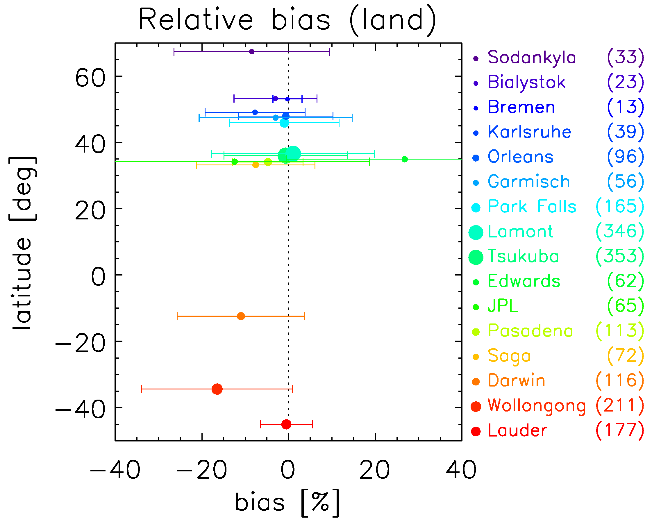
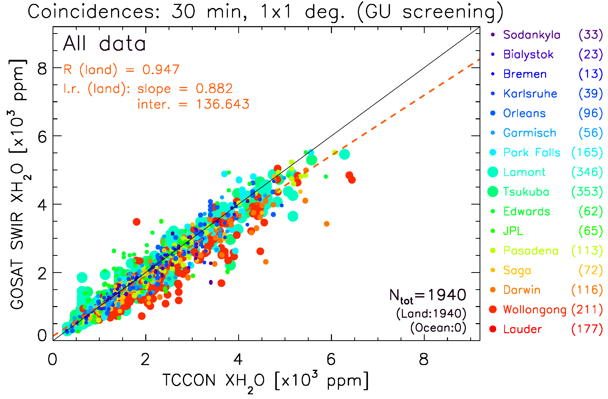
- We use the ground-based TCCON data as the reference for the calculations. The absolute bias for one pair (GOSAT vs. the mean of matched TCCON, “single-scan bias”) is thus defined as and the relative bias as the absolute bias ratioed to the TCCON values: . Here, represents the arithmetic mean of from all TCCON soundings coincident with one GOSAT scan. We then compute the corresponding global bias (absolute or relative, “ensemble bias”) as the arithmetic mean of the single-scan biases (absolute or relative) with its associated standard deviation. In order to evaluate the overall consistency of the results for different TCCON sites, the average and standard deviation of the station mean biases are also calculated (“station bias”). The linear least-squares fitting parameters and the correlation coefficient (R) are determined for the ensemble set and for each TCCON dataset.
- In this study, we directly compare the output of the NIES SWIR V02.21 and TCCON GGG2014 algorithms: no smoothing was applied to either dataset. Rigorously, comparison data should be smoothed following the approach of Rodgers and Connor [61], to account for the differences of instrumentation and observation geometries. The formalism of Rodgers [22], especially, provides and uses ad hoc mathematical tools—averaging kernels and a priori information—to perform this smoothing (e.g., [27,28,62]). However, smoothing the observed data might unduly constrain the comparison results towards the a priori information rather than towards the measured data, if the information content is low. Note that Inoue et al. [27] compared the NIES SWIR XCO retrievals to aircraft data with and without applying GOSAT averaging kernels to the higher-resolution aircraft data and did not find a significant difference for XCO.
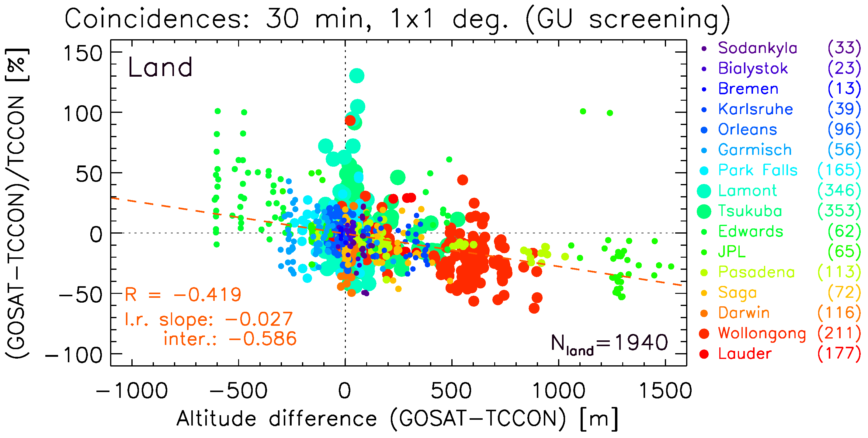
- Discrepancies between the mean altitude within a TANSO-FTS footprint and the elevation of the TCCON sites potentially have a significant impact on the results. This is particularly true for water vapor, whose column abundance is largely dominated by its lower-tropospheric amount. Here, we also assess the impact of the GOSAT/TCCON altitude differences on the XHO bias, but for simplicity reasons, we do not apply any altitude compensation to the GOSAT or TCCON columns prior to the bias calculations.
5. Results and Discussion
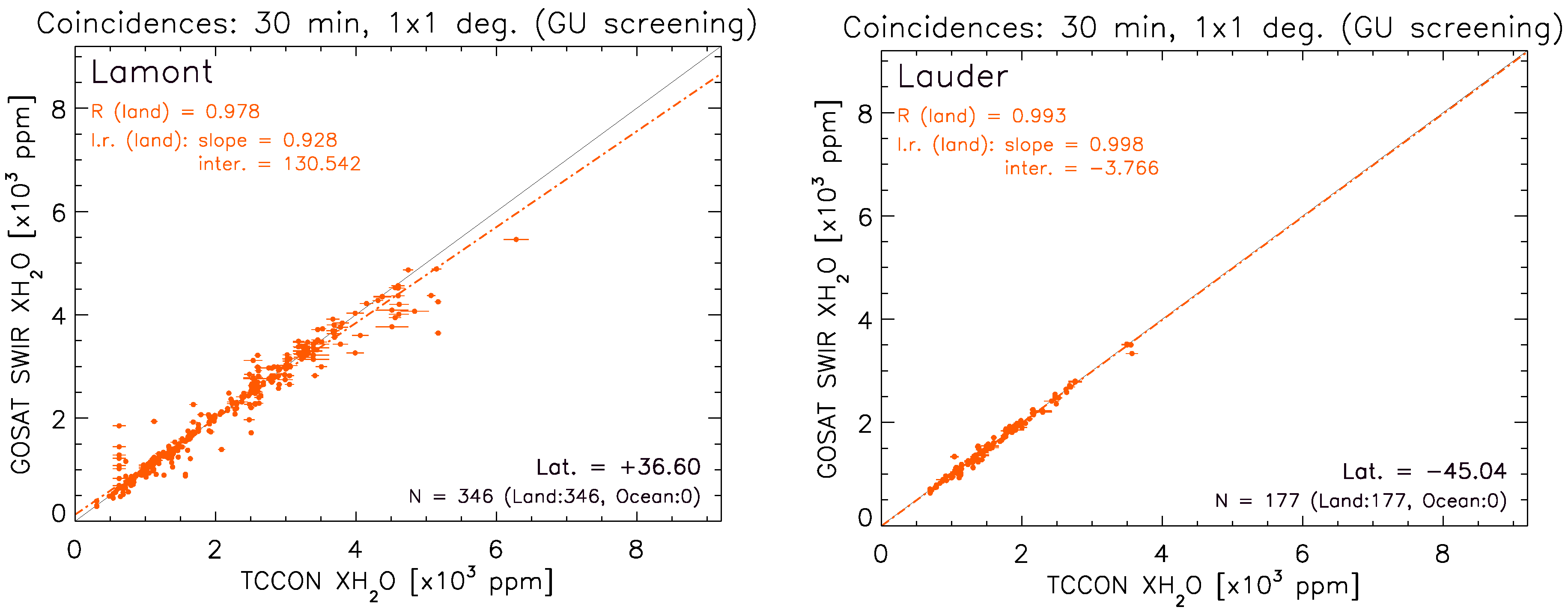
5.1. Statistical Comparison
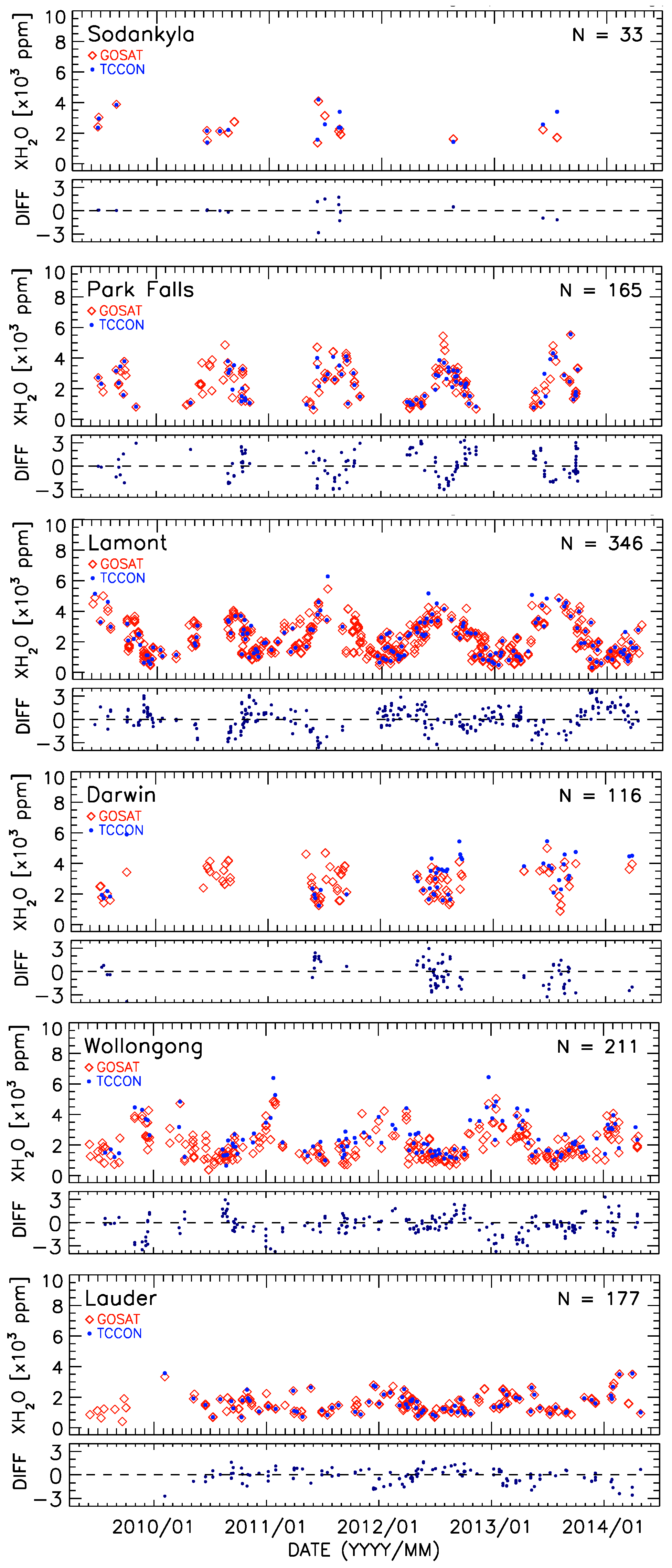
5.2. Temporal Evolution: Time Series for Selected Stations
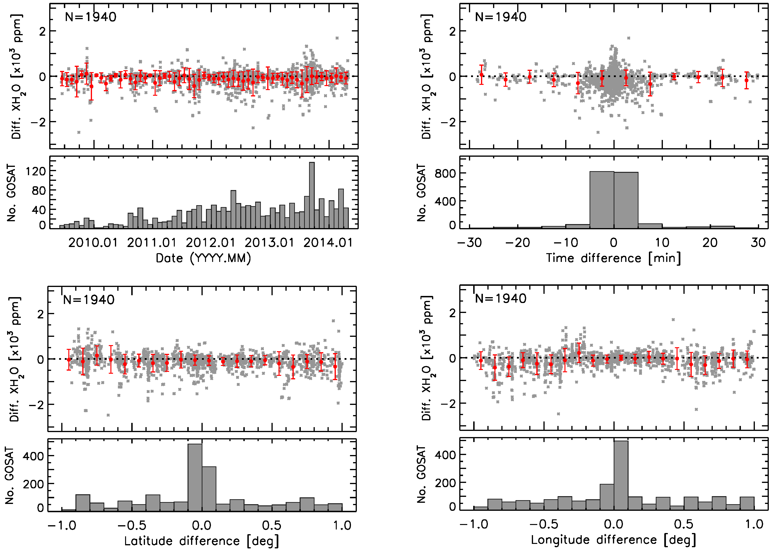
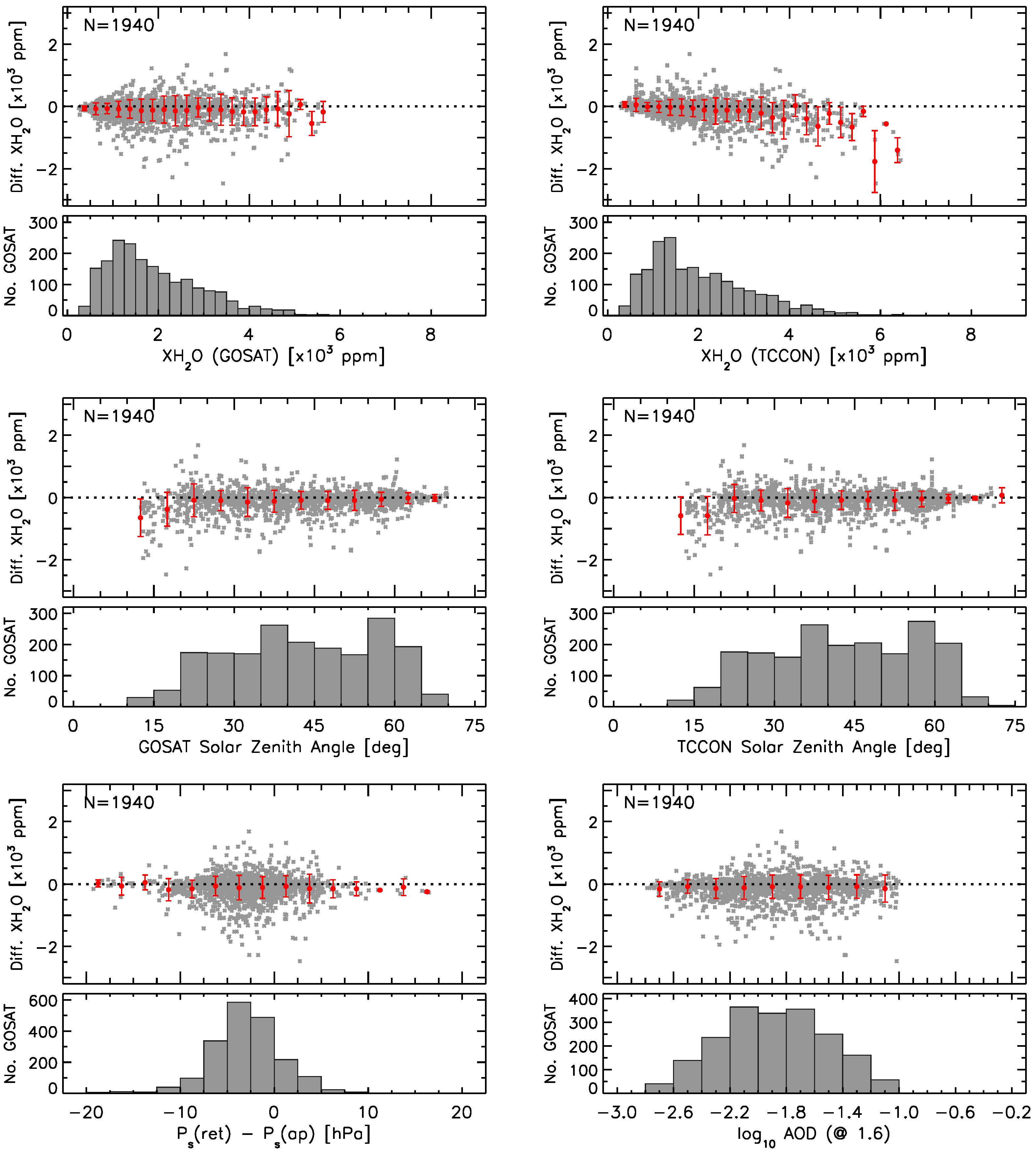
5.3. Impact of the Comparison Characteristics on the Single-Scan Differences
6. Conclusions
Supplementary Materials
Acknowledgments
Author Contributions
Conflicts of Interest
Appendix A

| Variable Tested | Code | Level | Rejection Condition | Explanation | ||
|---|---|---|---|---|---|---|
| Pre-Screening Items | ||||||
| L1B quality flag | l1q | RA, GU | l1q | = | 1 | Quality of the calibrated spectra |
| CAI radiances flag | cai | GU | cai | = | 1 | CAI coherence test |
| 2 m-scattering flag | mu2 | RA, GU | mu2 | = | 1 | High-altitude scattering |
| Solar zenith angle flag | sza | RA, GU | sza | = | 1 | Reject SZA larger than 70 |
| Land fraction | ldf | RA, GU | 0% < ldf | < | 60% | “Too mixed” ( land) |
| Signal-to-noise ratio | o2s | RA, GU | o2s | < | 70. | Minimum SNR in the O-A band |
| Post-Screening Items | ||||||
| Number of iterations | itr | RA, GU | itr | ≥ | 20 | Convergence not reached |
| Residuals Sub-band 1 | rb1 | RA | rb1 | ≥ | 1.4 | RMS Band 1 (O-A) |
| GU | ≥ | 1.2 | ||||
| Residuals Sub-band 2 | rb2 | RA | rb2 | ≥ | 1.5 | RMS Band 2 (wCO) |
| GU | ≥ | 1.2 | ||||
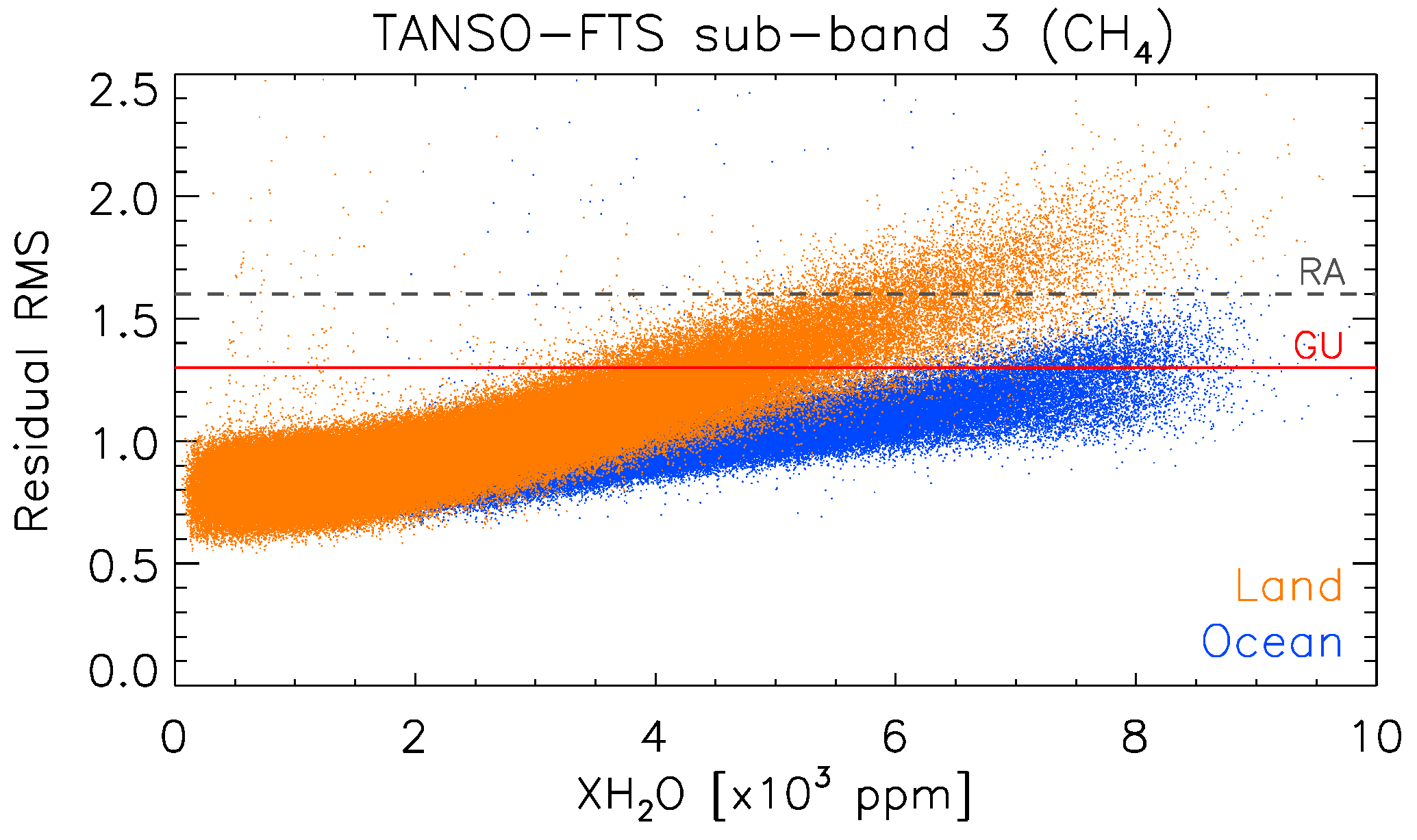
| Residuals Sub-band 3 | rb3 | RA | rb3 | ≥ | 1.6 | RMS Band 2 (CH) |
| GU | ≥ | 1.3 | ||||
| Residuals Sub-band 4 | rb4 | RA | rb4 | ≥ | 1.6 | RMS Band 3 (SCO) |
| GU | ≥ | 1.4 | ||||
| Degrees of freedom | dfs | RA | dfs | < | 0.8 | Minimum column information content |
| GU | < | 1. | ||||
| Aerosol optical thickness | aot | RA | aot | > | 0.5 | Estimated value at 1.6 μm |
| GU | > | 0.1 | ||||
| Blended albedo | bla | RA, GU | bla | ≥ | 1. | Land scans only |
| (if ldf ≥ 60.) | ||||||
| Surface wind speed | wsp | RA, GU | wsp | ≤ | 0.1 m.s | Ocean scans only |
| or wsp | ≥ | 20.1 m.s | (if ldf = 0.) | |||
| Retrieved surface pressure | dsp | RA, GU | dsp | > | 20.1 hPa | abs (retrieved − a priori) |
| Date selection | dtn | RA, GU | Earlier than 03 June 2003 | Operational period only | ||
References
- Trenberth, K.E. Atmospheric moisture residence times and cycling: Implications for rainfall rates and climate change. Clim. Chang. 1998, 39, 667–694. [Google Scholar] [CrossRef]
- Harries, J.E. Atmospheric radiation and atmospheric humidity. Quart. J. R. Meteor. Soc. 1997, 123, 2173–2186. [Google Scholar] [CrossRef]
- Trenberth, K.E.; Fasullo, J.; Smith, L. Trends and variability in column-integrated atmospheric water vapor. Clim. Dyn. 2005, 24, 741–758. [Google Scholar] [CrossRef]
- Worden, J.; Noone, D.; Bowman, K.; the Tropospheric Emission Spectrometer science team and data contributors. Importance of rain evaporation and continental convection in the tropical water cycle. Nature 2007, 445, 528–532. [Google Scholar] [CrossRef] [PubMed]
- Held, I.M.; Soden, B.J. Robust Responses of the Hydrological Cycle to Global Warming. J. Clim. 2006, 19, 5686–5699. [Google Scholar] [CrossRef]
- Flato, G.; Marotzke, J.; Braconnot, P.; Chou, S.C.; Collins, W.; Cox, P.; Driouech, F.; Emori, S.; Eyring, V.; Forest, C.; Stocker, T.F.; et al. Evaluation of Climate Models. In Climate Change 2013: The Physical Science Basis. Contribution of Working Group I to the Fifth Assessment Report of the Intergovernmental Panel on Climate Change; Stocker, T.F., Qin, D., Plattner, G.K., Tignor, M., Allen, S.K., Boschung, J., Nauels, A., Xia, Y., Bex, V., Midgley, P.M., Eds.; Cambridge University Press: Cambridge, UK; New York, NY, USA, 2013; pp. 741–866. [Google Scholar]
- Stocker, T.F.; Qin, D.; Plattner, G.K.; Alexander, L.V.; Allen, S.K.; Bindoff, N.L.; Bréon, F.M.; Church, J.A.; Cubasch, U.; Emori, S.; et al. Technical Summary. In Climate Change 2013: The Physical Science Basis. Contribution of Working Group I to the Fifth Assessment Report of the Intergovernmental Panel on Climate Change; Stocker, T.F., Qin, D., Plattner, G.K., Tignor, M., Allen, S.K., Boschung, J., Nauels, A., Xia, Y., Bex, V., Midgley, P.M., Eds.; Cambridge University Press: Cambridge, UK; New York, NY, USA, 2013; pp. 33–115. [Google Scholar]
- Vogelmann, H.; Sussmann, R.; Trickl, T.; Reichert, A. Spatiotemporal variability of water vapor investigated using lidar and FTIR vertical soundings above the Zugspitze. Atmos. Chem. Phys. 2015, 15, 3135–3148. [Google Scholar] [CrossRef]
- Sussmann, R.; Borsdorff, T.; Rettinger, M.; Camy-Peyret, C.; Demoulin, P.; Duchatelet, P.; Mahieu, E.; Servais, C. Technical Note: Harmonized retrieval of column-integrated atmospheric water vapor from the FTIR network–first examples for long-term records and station trends. Atmos. Chem. Phys. 2009, 9, 8987–8999. [Google Scholar] [CrossRef]
- Vogelmann, H.; Sussmann, R.; Trickl, T.; Borsdorff, T. Intercomparison of atmospheric water vapor soundings from the differential absorption lidar (DIAL) and the solar FTIR system on Mt. Zugspitze. Atmos. Meas. Tech. 2011, 4, 835–841. [Google Scholar] [CrossRef]
- Ross, R.J.; Elliott, W.P. Tropospheric Water Vapor Climatology and Trends over North America: 1973–1993. J. Clim. 1996, 9, 3561–3574. [Google Scholar] [CrossRef]
- Kämpfer, N. (Ed.) Monitoring Atmospheric Water Vapour; ISSI Scientific Report Series 10; Springer: New York, NY, USA, 2013.
- Urban, J. Satellite sensors measuring atmospheric water vapour. In Monitoring Atmospheric Water Vapour; ISSI Scientific Report Series 10; Kämpfer, N., Ed.; Springer: New York, NY, USA, 2013; pp. 175–214. [Google Scholar]
- Buehler, S.A.; Östman, S.; Melsheimer, C.; Holl, G.; Eliasson, S.; John, V.O.; Blumenstock, T.; Hase, F.; Elgered, G.; Raffalski, U.; et al. A multi-instrument comparison of integrated water vapour measurements at a high latitude site. Atmos. Chem. Phys. 2012, 12, 10925–10943. [Google Scholar] [CrossRef]
- Van Malderen, R.; Brenot, H.; Pottiaux, E.; Beirle, S.; Hermans, C.; De Mazière, M.; Wagner, T.; De Backer, H.; Bruyninx, C. A multi-site intercomparison of integrated water vapour observations for climate change analysis. Atmos. Meas. Tech. 2014, 7, 2487–2512. [Google Scholar] [CrossRef]
- Kuze, A.; Suto, H.; Shiomi, K.; Nakajima, M.; Hamazaki, T. On-orbit performance and Level 1 data processing of TANSO-FTS and CAI on GOSAT. Proc. SPIE 2009, 7474. [Google Scholar] [CrossRef]
- Yoshida, Y.; Kikuchi, N.; Morino, I.; Uchino, O.; Oshchepkov, S.; Bril, A.; Saeki, T.; Schutgens, N.; Toon, G.C.; Wunch, D.; et al. Improvement of the retrieval algorithm for GOSAT SWIR XCO2 and XCH4 and their validation using TCCON data. Atmos. Meas. Tech. 2013, 6, 1533–1547. [Google Scholar] [CrossRef]
- Wunch, D.; Toon, G.C.; Blavier, J.F.L.; Washenfelder, R.A.; Notholt, J.; Connor, B.J.; Griffith, D.W.T.; Sherlock, V.; Wennberg, P.O. The Total Carbon Column Observing Network. Phil. Trans. R. Soc. A 2011, 369, 2087–2112. [Google Scholar] [CrossRef] [PubMed]
- Butz, A.; Hasekamp, O.P.; Frankenberg, C.; Aben, I. Retrievals of atmospheric CO2 from simulated space-borne measurements of backscattered near-infrared sunlight: accounting for aerosol effects. Atmos. Ocean 2009, 48, 3322–3336. [Google Scholar]
- Yoshida, Y.; Ota, Y.; Eguchi, N.; Kikuchi, N.; Nobuta, K.; Tran, H.; Morino, I.; Yokota, T. Retrieval algorithm for CO2 and CH4 column abundances from short-wavelength infrared spectral observations by the Greenhouse gases observing satellite. Atmos. Meas. Tech. 2011, 4, 717–734. [Google Scholar] [CrossRef]
- Ishida, H.; Nakajima, T.Y. Development of an unbiased cloud detection algorithm for a spaceborne multispectral imager. J. Geophys. Res. Atmos. 2009, 114, D07206. [Google Scholar] [CrossRef]
- Rodgers, C.D. Inverse Methods for Atmospheric Sounding—Theory and Practise; Series on Atmospheric, Oceanic and Planetary Physics; World Scientific: Singapore, 2000; Volume 2. [Google Scholar]
- Rothman, L.; Gordon, I.E.; Barbe, A.; Benner, D.C.; Bernath, P.F.; Birk, M.; Boudon, V.; Brown, L.R.; Campargue, A.; Champion, J.P.; et al. The HITRAN 2008 molecular spectroscopic database. J. Quant. Spectrosc. Radiat. Transf. 2009, 110, 533–572. [Google Scholar] [CrossRef]
- Takemura, H.; Egashira, M.; Matsuzawa, K.; Ichijo, H.; O’ishi, R.; Abe-Ouchi, A. A simulation of the global distribution and radiative forcing of soil dust aerosols at the Last Glacial Maximum. Atmos. Chem. Phys. 2015, 9, 3061–3073. [Google Scholar] [CrossRef]
- The GOSAT User Interface Gateway. Available online: http://data.gosat.nies.go.jp/ (accessed on 9 May 2016).
- Morino, I.; Uchino, O.; Inoue, M.; Yoshida, Y.; Yokota, T.; Wennberg, P.O.; Toon, G.C.; Wunch, D.; Roehl, C.M.; Notholt, J.; et al. Preliminary validation of column-averaged volume mixing ratios of carbon dioxide and methane retrieved from GOSAT short-wavelength infrared spectra. Atmos. Meas. Tech. 2011, 4, 1061–1076. [Google Scholar] [CrossRef]
- Inoue, M.; Morino, I.; Uchino, O.; Miyamoto, Y.; Yoshida, Y.; Yokota, T.; Machida, T.; Sawa, Y.; Matsueda, H.; Sweeney, C.; et al. Validation of XCO2 derived from SWIR spectra of GOSAT TANSO-FTS with aircraft measurement data. Atmos. Chem. Phys. 2013, 13, 9771–9788. [Google Scholar] [CrossRef]
- Inoue, M.; Morino, I.; Uchino, O.; Miyamoto, Y.; Saeki, T.; Yoshida, Y.; Yokota, T.; Sweeney, C.; Tans, P.P.; Biraud, S.C.; et al. Validation of XCH4 derived from SWIR spectra of GOSAT TANSO-FTS with aircraft measurement data. Atmos. Meas. Tech. 2014, 7, 2987–3005. [Google Scholar] [CrossRef]
- Frankenberg, C.; Wunch, D.; Toon, G.; Risi, C.; Scheepmaker, R.; Lee, J.E.; Wennberg, P.; Worden, J. Water vapor isotopologue retrievals from high-resolution GOSAT shortwave infrared spectra. Atmos. Meas. Tech. 2013, 6, 263–274. [Google Scholar] [CrossRef] [Green Version]
- Boesch, H.; Deutscher, N.M.; Warneke, T.; Byckling, K.; Cogan, A.J.; Griffith, D.W.T.; Notholt, J.; Parker, R.J.; Wang, Z. HDO/H2O ratio retrievals from GOSAT. Atmos. Meas. Tech. 2013, 6, 599–612. [Google Scholar] [CrossRef]
- O’Dell, C.W.; Connor, B.; Bösch, H.; O’Brien, D.; Frankenberg, C.; Castano, R.; Christi, M.; Eldering, D.; Fisher, B.; Gunson, M.; et al. The ACOS CO2 retrieval algorithm—Part 1: Description and validation against synthetic observations. Atmos. Meas. Tech. 2012, 5, 99–121. [Google Scholar] [CrossRef]
- Butz, A.; Guerlet, S.; Hasekamp, O.; Schepers, D.; Galli, A.; Aben, I.; Frankenberg, C.; Hartmann, J.M.; Tran, H.; Kuze, A.; et al. Toward accurate CO2 and CH4 observations from GOSAT. Geophys. Res. Lett. 2011, 38, L14812. [Google Scholar] [CrossRef]
- Wunch, D.; Toon, G.C.; Wennberg, P.O.; Wofsy, S.C.; Stephens, B.B.; Fischer, M.L.; Uchino, O.; Abshire, J.B.; Bernath, P.; Biraud, S.C.; et al. Calibration of the Total Carbon Column Observing Network using aircraft profile data. Atmos. Meas. Tech. 2010, 3, 1351–1362. [Google Scholar] [CrossRef]
- The TCCON Data Archive. Available online: http://tccon.ornl.gov/ (accessed on 9 May 2016).
- The TCCON-Wiki Website. Available online: http://tccon-wiki.caltech.edu/ (accessed on 9 May 2016).
- Kivi, R.; Heikkinen, P.; Kyrö, E. TCCON Data from Sodankylä, Finland, Release GGG2014R0; Carbon Dioxide Information Analysis Center; Oak Ridge National Laboratory: Oak Ridge, TN, USA, 2014. [Google Scholar] [CrossRef]
- Deutscher, N.; Notholt, J.; Messerschmidt, J.; Weinzierl, C.; Warneke, T.; Petri, C.; Grupe, P.; Katrynski, K. TCCON Data from Bialystok, Poland, Release GGG2014R1; Carbon Dioxide Information Analysis Center; Oak Ridge National Laboratory: Oak Ridge, TN, USA, 2014. [Google Scholar] [CrossRef]
- Notholt, J.; Petri, C.; Warneke, T.; Deutscher, N.; Buschmann, M.; Weinzierl, C.; Macatangay, R.; Grupe, P. TCCON Data from Bremen, Germany, Release GGG2014R0; Carbon Dioxide Information Analysis Center; Oak Ridge National Laboratory: Oak Ridge, TN, USA, 2014. [Google Scholar] [CrossRef]
- Hase, F.; Blumenstock, T.; Dohe, S.; Groß, J.; Kiel, M. TCCON Data from Karlsruhe, Germany, Release GGG2014R1; Carbon Dioxide Information Analysis Center; Oak Ridge National Laboratory: Oak Ridge, TN, USA, 2014. [Google Scholar] [CrossRef]
- Warneke, T.; Messerschmidt, J.; Notholt, J.; Weinzierl, C.; Deutscher, N.; Petri, C.; Grupe, P.; Vuillemin, C.; Truong, F.; Schmidt, M.; Ramonet, M.; Parmentier, E. TCCON Data from Orléans, France, Release GGG2014R0; Carbon Dioxide Information Analysis Center; Oak Ridge National Laboratory: Oak Ridge, TN, USA, 2014. [Google Scholar] [CrossRef]
- Sussmann, R.; Rettinger, M. TCCON Data from Garmisch, Germany, Release GGG2014R0; Carbon Dioxide Information Analysis Center; Oak Ridge National Laboratory: Oak Ridge, TN, USA, 2014. [Google Scholar] [CrossRef]
- Wennberg, P.O.; Roehl, C.; Wunch, D.; Toon, G.C.; Blavier, J.F.; Washenfelder, R.; Keppel-Aleks, G.; Allen, N.; Ayers, J. TCCON Data from Park Falls, Wisconsin, USA, Release GGG2014R0; Carbon Dioxide Information Analysis Center; Oak Ridge National Laboratory: Oak Ridge, TN, USA, 2014. [Google Scholar] [CrossRef]
- Iraci, L.; Podolske, J.; Hillyard, P.; Roehl, C.; Wennberg, P.O.; Blavier, J.F.; Landeros, J.; Allen, N.; Wunch, D.; Zavaleta, J.; et al. TCCON Data from Indianapolis, Indiana, USA, Release GGG2014R0; Carbon Dioxide Information Analysis Center; Oak Ridge National Laboratory: Oak Ridge, TN, USA, 2014. [Google Scholar] [CrossRef]
- Wennberg, P.O.; Wunch, D.; Roehl, C.; Blavier, J.F.; Toon, G.C.; Allen, N.; Dowell, P.; Teske, K.; Martin, C.; Martin, J. TCCON Data from Lamont, Oklahoma, USA, Release GGG2014R0; Carbon Dioxide Information Analysis Center; Oak Ridge National Laboratory: Oak Ridge, TN, USA, 2014. [Google Scholar] [CrossRef]
- Morino, I.; Matsuzaki, T.; Ikegami, H.; Shishime, A. TCCON Data from Tsukuba, Ibaraki, Japan, 125 HR, Release GGG2014R0; Carbon Dioxide Information Analysis Center; Oak Ridge National Laboratory: Oak Ridge, TN, USA, 2014. [Google Scholar] [CrossRef]
- Iraci, L.; Podolske, J.; Hillyard, P.; Roehl, C.; Wennberg, P.O.; Blavier, J.F.; Landeros, J.; Allen, N.; Wunch, D.; Zavaleta, J.; et al. TCCON Data from Armstrong Flight Research Center, Edwards, CA, USA, Release GGG2014R0; Carbon Dioxide Information Analysis Center; Oak Ridge National Laboratory: Oak Ridge, TN, USA, 2014. [Google Scholar] [CrossRef]
- Wennberg, P.O.; Roehl, C.; Blavier, J.F.; Wunch, D.; Landeros, J.; Allen, N. TCCON Data from Jet Propulsion Laboratory, Pasadena, California, USA, Release GGG2014R0; Carbon Dioxide Information Analysis Center; Oak Ridge National Laboratory: Oak Ridge, TN, USA, 2014. [Google Scholar] [CrossRef]
- Wennberg, P.O.; Wunch, D.; Roehl, C.; Blavier, J.F.; Toon, G.C.; Allen, N. TCCON Data from California Institute of Technology, Pasadena, California, USA, Release GGG2014R1; Carbon Dioxide Information Analysis Center; Oak Ridge National Laboratory: Oak Ridge, TN, USA, 2014. [Google Scholar] [CrossRef]
- Shiomi, K.; Kawakami, S.; Ohyama, H.; Arai, K.; Okumura, H.; Taura, C.; Fukamachi, T.; Sakashita, M. TCCON Data from Saga, Japan, Release GGG2014R0; Carbon Dioxide Information Analysis Center; Oak Ridge National Laboratory: Oak Ridge, TN, USA, 2014. [Google Scholar] [CrossRef]
- Griffith, D.W.T.; Deutscher, N.; Velazco, V.A.; Wennberg, P.O.; Yavin, Y.; Keppel-Aleks, G.; Washenfelder, R.; Toon, G.C.; Blavier, J.F.; Murphy, C.; et al. TCCON Data from Darwin, Australia, Release GGG2014R0; Carbon Dioxide Information Analysis Center; Oak Ridge National Laboratory: Oak Ridge, TN, USA, 2014. [Google Scholar] [CrossRef]
- De Mazière, M.; Desmet, F.; Hermans, C.; Scolas, F.; Kumps, N.; Metzger, J.M.; Duflot, V.; Cammas, J.P. TCCON Data from Reunion Island (La Réunion), France, Release GGG2014R0; Carbon Dioxide Information Analysis Center; Oak Ridge National Laboratory: Oak Ridge, TN, USA, 2014. [Google Scholar] [CrossRef]
- Griffith, D.W.T.; Velazco, V.A.; Deutscher, N.; Murphy, C.; Jones, N.; Wilson, S.; Macatangay, R.; Kettlewell, G.; Buchholz, R.R.; Riggenbach, M. TCCON Data from Wollongong, Australia, Release GGG2014R0; Carbon Dioxide Information Analysis Center; Oak Ridge National Laboratory: Oak Ridge, TN, USA, 2014. [Google Scholar] [CrossRef]
- Sherlock, V.; Connor, B.; Robinson, J.; Shiona, H.; Smale, D.; Pollard, D. TCCON Data from Lauder, New Zealand, 125 HR, Release GGG2014R0; Carbon Dioxide Information Analysis Center; Oak Ridge National Laboratory: Oak Ridge, TN, USA, 2014. [Google Scholar] [CrossRef]
- The TCCON Sites: Dryden/Armstrong/Edwards. Available online: http://tccon-wiki.caltech.edu/Sites/Dryden (accessed on 10 May 2016).
- Toon, G.C.; Blavier, J.F.; Sen, B.; Salawitch, R.J.; Osterman, G.B.; Notholt, J.; Rex, M.; McElroy, C.T.; Russell, J.M., III. Ground-based observations of Arctic ozone loss during spring and summer 1997. J. Geophys. Res. 1999, 104, 26497–26510. [Google Scholar] [CrossRef]
- Wunch, D.; Toon, G.C.; Sherlock, V.; Deutscher, N.M.; Liu, X.; Feist, D.G.; Wennberg, P.O. The Total Carbon Column Observing Network’s GGG2014 Data Version, 2015; Carbon Dioxide Information Analysis Center, Oak Ridge National Laboratory: Oak Ridge, TN, USA, 2015; Available online: http://0-dx-doi-org.brum.beds.ac.uk/10.14291/tccon.ggg2014.documentation.R0/1221662 (accessed on 10 May 2016).
- Messerschmidt, J.; Geibel, M.C.; Blumenstock, T.; Chen, H.; Deutscher, N.M.; Engel, A.; Feist, D.G.; Gerbig, C.; Gisi, M.; Hase, F.; et al. Calibration of TCCON column-averaged CO2: The first aircraft campaign over European TCCON sites. Atmos. Chem. Phys. 2011, 11, 10765–10777. [Google Scholar] [CrossRef]
- Geibel, M.C.; Messerschmidt, J.; Gerbig, C.; Blumenstock, T.; Chen, H.; Hase, F.; Kolle, O.; Lavrič, J.V.; Notholt, J.; Palm, M.; et al. Calibration of column-averaged CH4 over European TCCON FTS sites with airborne in-situ measurements. Atmos. Chem. Phys. 2012, 12, 8763–8775. [Google Scholar] [CrossRef]
- Yoshida, Y.; Kikuchi, N.; Inoue, M.; Morino, I.; Uchino, O.; Yokota, T. Recent Topics about the GOSAT TANSO-FTS SWIR L2 Retrievals. AGU Fall Meet. Abstr. 2014, 1, 3154. [Google Scholar]
- The TCCON Data Description: Site-Specific Notes. Available online: https://tccon-wiki.caltech.edu/Network_Policy/Data_Use_Policy/Data_DescriptionSITE-SPECIFIC_NOTES (accessed on 10 May 2016).
- Rodgers, C.D.; Connor, B.J. Intercomparison of remote sounding instruments. J. Geophys. Res. Atmos. 2003, 108, 4116–4129. [Google Scholar] [CrossRef]
- Wunch, D.; Wennberg, P.O.; Toon, G.C.; Connor, B.J.; Fisher, B.; Osterman, G.B.; Frankenberg, C.; Mandrake, L.; O’Dell, C.; Ahonen, P.; et al. A method for evaluating bias in global measurements of CO2 total columns from space. Atmos. Chem. Phys. 2011, 11, 12317–12337. [Google Scholar] [CrossRef]
- Du Piesanie, A.; Piters, A.J.M.; Aben, I.; Schrijver, H.; Wang, P.; Noël, S. Validation of two independent retrievals of SCIAMACHY water vapour columns using radiosonde data. Atmos. Meas. Tech. 2013, 6, 2925–2940. [Google Scholar] [CrossRef]
- Wagner, T.; Andreae, M.O.; Beirle, S.; Dörner, S.; Mies, K.; Shaiganfar, R. MAX-DOAS observations of the total atmospheric water vapour column and comparison with independent observations. Atmos. Meas. Tech. 2013, 6, 131–149. [Google Scholar] [CrossRef]
- Palm, M.; Melsheimer, C.; Noël, S.; Heise, S.; Notholt, J.; Burrows, J.; Schrems, O. Integrated water vapor above Ny Ålesund, Spitsbergen: A multi-sensor intercomparison. Atmos. Chem. Phys. 2010, 10, 1215–1226. [Google Scholar] [CrossRef]


| Site/Dataset | Latitude | Longitude | Altitude | Start/End of | Reference | |
|---|---|---|---|---|---|---|
| () | () | (km) | Operations | |||
| Sodankylä | 67.37 | 26.63 | 0.188 | 6 February 2009 | Ongoing | Kivi et al. [36] |
| Bialystok | 53.23 | 23.03 | 0.180 | 1 March 2009 | Ongoing | Deutscher et al. [37] |
| Bremen | 53.10 | 8.85 | 0.030 | 6 January 2005 | Ongoing | Notholt et al. [38] |
| Karlsruhe | 49.10 | 8.44 | 0.119 | 19 April 2010 | Ongoing | Hase et al. [39] |
| Orléans | 47.97 | 2.11 | 0.130 | 29 August 2009 | Ongoing | Warneke et al. [40] |
| Garmisch | 47.48 | 11.06 | 0.743 | 16 July 2007 | Ongoing | Sussmann et al. [41] |
| Park Falls | 45.95 | −90.27 | 0.442 | 26 May 2004 | Ongoing | Wennberg et al. [42] |
| Indianapolis | 39.86 | −86.00 | 0.270 | 23 August 2012 | 1 December 2012 | Iraciet al. [43] |
| Lamont | 36.60 | −97.49 | 0.320 | 6 July 2008 | Ongoing | Wennberg et al. [44] |
| Tsukuba | 36.05 | 140.12 | 0.031 | 4 August 2011 | Ongoing | Morino et al. [45] |
| Edwards | 34.96 | −117.88 | 0.700 | 20 July 2013 | Ongoing | Iraci et al. [46] |
| JPL | 34.20 | −118.18 | 0.390 | 8 December 2011 | 31 March 2013 | Wennberg et al. [47] |
| Pasadena | 34.14 | −118.13 | 0.230 | 20 September 2012 | Ongoing | Wennberg et al. [48] |
| Saga | 33.24 | 130.29 | 0.007 | 28 July 2011 | Ongoing | Shiomi et al. [49] |
| Darwin | −12.42 | 130.89 | 0.030 | 28 August 2005 | June 2015 | Griffith et al. [50] |
| −12.46 | 130.93 | 0.037 | June 2015 | Ongoing | ||
| La Réunion | −20.90 | 55.49 | 0.087 | 6 October 2011 | Ongoing | De Mazière et al. [51] |
| Wollongong | −34.41 | 150.88 | 0.030 | 26 June 2008 | Ongoing | Griffith et al. [52] |
| Lauder | −45.04 | 169.68 | 0.370 | 2 February 2010 | Ongoing | Sherlock et al. [53] |
| TCCON | # of Scans | Bias ± SD | Bias ± SD |
|---|---|---|---|
| Dataset | (ppm) | (%) | |
| Sodankylä | 33 | −264.0 ± 548.6 | −8.50 ± 17.93 |
| Bialystok | 23 | −106.6 ± 265.1 | −3.03 ± 9.56 |
| Bremen | 13 | 2.6 ± 53.2 | −0.26 ± 3.36 |
| Karlsruhe | 39 | −199.1 ± 303.0 | −7.74 ± 11.54 |
| Orléans | 96 | −11.3 ± 247.0 | −0.64 ± 10.89 |
| Garmisch | 56 | −120.9 ± 346.6 | −2.98 ± 17.65 |
| Park Falls | 165 | −25.7 ± 289.6 | −0.97 ± 12.62 |
| Lamont | 346 | −20.0 ± 239.6 | 1.06 ± 18.76 |
| Tsukuba | 353 | −28.9 ± 203.0 | −0.66 ± 14.26 |
| Edwards | 62 | 380.7 ± 410.5 | 26.79 ± 27.23 |
| JPL | 65 | −299.3 ± 574.9 | −12.45 ± 31.18 |
| Pasadena | 113 | −107.1 ± 180.4 | −4.77 ± 8.11 |
| Saga | 72 | −155.9 ± 289.6 | −7.60 ± 13.67 |
| Darwin | 116 | −389.7 ± 536.0 | −10.98 ± 14.71 |
| Wollongong | 211 | −410.1 ± 438.7 | −16.50 ± 17.43 |
| Lauder | 177 | −6.9 ± 75.7 | −0.51 ± 5.99 |
| Ensemble bias | 1940 | −103.2 ± 356.5 | −3.09 ± 17.72 |
| Station bias | 16 | −110.1 ± 188.6 | −3.11 ± 9.47 |
| TCCON | # of Scans | Slope | Intercept | R |
|---|---|---|---|---|
| Dataset | (ppm/ppm) | (ppm) | ||
| Sodankylä | 33 | 0.75 | 368.1 | 0.77 |
| Bialystok | 23 | 0.93 | 62.7 | 0.97 |
| Bremen | 13 | 1.02 | −24.8 | 1.00 |
| Karlsruhe | 39 | 0.88 | 82.6 | 0.97 |
| Orléans | 96 | 0.99 | 8.0 | 0.97 |
| Garmisch | 56 | 0.89 | 104.3 | 0.95 |
| Park Falls | 165 | 0.99 | 7.7 | 0.96 |
| Lamont | 346 | 0.93 | 130.5 | 0.98 |
| Tsukuba | 353 | 0.94 | 53.4 | 0.97 |
| Edwards | 62 | 0.91 | 557.5 | 0.94 |
| JPL | 65 | 0.70 | 297.2 | 0.75 |
| Pasadena | 113 | 0.94 | 17.4 | 0.99 |
| Saga | 72 | 0.92 | 4.9 | 0.97 |
| Darwin | 116 | 0.70 | 519.0 | 0.87 |
| Wollongong | 211 | 0.83 | 10.0 | 0.93 |
| Lauder | 177 | 1.00 | −3.8 | 0.99 |
| Ensemble bias | 1940 | 0.88 | 136.7 | 0.95 |
| Station bias | 16 | 0.72 | 491.9 | 0.87 |
© 2016 by the authors; licensee MDPI, Basel, Switzerland. This article is an open access article distributed under the terms and conditions of the Creative Commons Attribution (CC-BY) license (http://creativecommons.org/licenses/by/4.0/).
Share and Cite
Dupuy, E.; Morino, I.; Deutscher, N.M.; Yoshida, Y.; Uchino, O.; Connor, B.J.; De Mazière, M.; Griffith, D.W.T.; Hase, F.; Heikkinen, P.; et al. Comparison of XH2O Retrieved from GOSAT Short-Wavelength Infrared Spectra with Observations from the TCCON Network. Remote Sens. 2016, 8, 414. https://0-doi-org.brum.beds.ac.uk/10.3390/rs8050414
Dupuy E, Morino I, Deutscher NM, Yoshida Y, Uchino O, Connor BJ, De Mazière M, Griffith DWT, Hase F, Heikkinen P, et al. Comparison of XH2O Retrieved from GOSAT Short-Wavelength Infrared Spectra with Observations from the TCCON Network. Remote Sensing. 2016; 8(5):414. https://0-doi-org.brum.beds.ac.uk/10.3390/rs8050414
Chicago/Turabian StyleDupuy, Eric, Isamu Morino, Nicholas M. Deutscher, Yukio Yoshida, Osamu Uchino, Brian J. Connor, Martine De Mazière, David W. T. Griffith, Frank Hase, Pauli Heikkinen, and et al. 2016. "Comparison of XH2O Retrieved from GOSAT Short-Wavelength Infrared Spectra with Observations from the TCCON Network" Remote Sensing 8, no. 5: 414. https://0-doi-org.brum.beds.ac.uk/10.3390/rs8050414