Effects of Spatial Sampling Interval on Roughness Parameters and Microwave Backscatter over Agricultural Soil Surfaces

Abstract

The spatial sampling interval, as related to the ability to digitize a soil profile with a certain number of features per unit length, depends on the profiling technique itself. From a variety of profiling techniques, roughness parameters are estimated at different sampling intervals. Since soil profiles have continuous spectral components, it is clear that roughness parameters are influenced by the sampling interval of the measurement device employed. In this work, we contributed to answer which sampling interval the profiles needed to be measured at to accurately account for the microwave response of agricultural surfaces. For this purpose, a 2-D laser profiler was built and used to measure surface soil roughness at field scale over agricultural sites in Argentina. Sampling intervals ranged from large (50 mm) to small ones (1 mm), with several intermediate values. Large- and intermediate-sampling-interval profiles were synthetically derived from nominal, 1 mm ones. With these data, the effect of sampling-interval-dependent roughness parameters on backscatter response was assessed using the theoretical backscatter model IEM2M. Simulations demonstrated that variations of roughness parameters depended on the working wavelength and was less important at L-band than at C- or X-band. In any case, an underestimation of the backscattering coefficient of about 1-4 dB was observed at larger sampling intervals. As a general rule a sampling interval of 15 mm can be recommended for L-band and 5 mm for C-band.

1. Introduction

It is well-established the importance of accurately accounting for surface roughness conditions over agricultural lands as a requirement for retrieving near-surface soil moisture from microwave remotely-sensed Synthetic Aperture Radar (SAR) images. Despite the fact that there are a number of intrinsic roughness-related applications, such as in agricultural studies (e.g., monitoring tillage activities, crop residue cover, etc.) [1] and in geological surveys (e.g., characterization and classification of lava flows, alluvial deposits, desert surfaces, etc.) [2], roughness is mostly understood as a disturbing factor in what respects to soil moisture estimation from SAR imagery. The reason is that the dynamic range of the backscatter response due to surface roughness is comparable to that of near-surface soil moisture. From a model standpoint, this soil roughness can be considered as the stochastic varying height of the soil surface towards a reference surface [3] (Volume II). This reference surface can be the unperturbed surface of a periodic pattern or can be the mean surface if only random variations exist.

In dealing with microwave remote sensing a range of surface roughness components are involved in the scattering response of agricultural lands. In fact, roughness can be considered as the sum of different soil components corresponding to different scales [4]:

(a)

a small scale (millimeter to centimeter scale) involving grains, individual soil aggregates and soil clods, which represent a non-oriented, random component;

(b)

a medium scale (centimeter to decimeter scale) related to furrows or tillage rows, which represent an oriented, periodic, deterministic component; and

(c)

a large scale (decimeter to meter, pixel-sized scale) related to local topographic trends such as field slope, which defines the aspect of the land surface relative to the observation geometry of the sensor.

In terms of the sensor wavelength λ and for soil moisture applications (i.e., in the microwave portion of the spectrum), the random component involves dimensions of roughly $\frac{\lambda }{10}$ and contributes mostly with the incoherent component of the total scattered energy, whereas the periodic pattern of the medium scale, with dimensions of about λ, mainly accounts for the coherent component. The large scale (~10λ) determines the local incidence angle which in turn affect both the coherent and the incoherent components [3,5] (Chapter 12). In opposite to the large-scale (natural) component, both small- and medium-scale (man-made) components arise from tillage operations over the soil and are affected by weathering and erosion processes such as rainfall, runoff and wind.

The statistical properties of the soil roughness random component may be summarized using only two parameters derived from one-dimensional (1-D) profiles: the surface height standard deviation (s) and the surface correlation length (l), once the shape of the autocorrelation function (ACF) has been fixed. The height standard deviation describes the random variation in surface elevation with respect to a predefined reference surface, this being the mean plane when neither furrow structure nor tillage pattern are present. The autocorrelation function measures the degree of spatial dependence between points, whereas the correlation length indicates at what extent two separate points can be considered correlated. A complementary way to characterize 1-D rough profiles is through its power spectral density, which states the relative strength of the spatial frequencies present in the profile.

There are a number of limiting factors in the accuracy of surface roughness parameters as derived from profiling techniques, such as the profile length or measurement extent and the sampling interval or sampling distance, the later being the spacing between two contiguous height measurements. As for the profile length, for instance, experimental and numerical studies [6,7,8] suggested the need for long profiles ($400l$ or ~25 $\mathrm{m}$) whereas other studies, focused on soil moisture retrieval rather than on soil roughness measurements [9,10,11,12,13,14], employed 1-m-long profiles, where no clear relationship between the reliability of the retrieved estimates and the profile length could be found. As for the sampling interval $\Delta x$, a rule of thumb recommended in [3] (Volume II) stated that $\Delta x<\frac{\lambda }{10}$ provided that the corresponding change in height z is $\Delta z\ll \lambda$. This rule along with the Fraunhoffer criterion (which states that for smooth surfaces $s<\frac{\lambda }{32\cos \left(\theta \right)}$) [3,15] leads to an upper bound $\Delta x<2.3$ cm for a smooth surface ($s<0.94\mathrm{cm}$) imaged by an L-band ($\lambda =0.23\mathrm{m}$) sensor at $\theta =40°$. On the other hand, numerical experiments with synthesized rough surfaces were used to assess the impact of the sampling interval on the accuracy of roughness parameters. According to [16], the sampling interval should not exceed 0.1 times the actual (or true) correlation length (l) for accurate parameterization of roughness. Larger sampling interval instruments cause that the roughness profile is sampled at an insufficient rate and therefore, very small structures are not presented in the obtained roughness profile. This subsampling mainly causes a change in slope of the ACF around zero [16]. In this sense, in [6] it is stated that the sampling interval should be smaller than $0.2l$ for the roughness parameters to be estimated within 5% error. It is worth mentioning the lack of experimental studies in this respect, with the exception of [17] where such a study was performed over an experimental bare soil patch.

Typical in-situ roughness measurement methods at field scale involve the use of contact profilers such as pinmeters or meshboards [18]. More advanced profiling methods use non-contact, laser techniques such as triangulation [19,20] or time-of-flight distance meters [7]. In the triangulation laser techniques, each laser-illuminated soil feature is recorded onto a picture by a camera and then transformed to a reference frame using a dedicated calibration procedure. The calibration procedure sets a polynomial transformation from pixel coordinates to millimeter coordinates in the reference frame. By means of a moving platform, contiguous pictures of adjacent soil features are recorded. Therefore, the sampling interval of the soil profiles is given by the sampling distance of the laser survey over the surface, providing non-overlapping measurements are performed. In the same way, the sampling interval in time-of-flight techniques is simply defined by the distance between two contiguous measurements the distance meter is positioned at. Using these techniques, measured profiles have generally a length between 1 m and 4 m, and a sampling interval between 1 mm and 20 mm [18].

A valuable advantage of these laser techniques is that they are self-contained, yielding a high portability to their corresponding instruments that enables collecting multisite measurements over relative large extents. This is important, since recently-developed methods involving close range techniques, such as stereo-photogrammetric systems (see for instance [21]), Structure from Motion [22] or Terrestrial Laser Scanning [17] are more suitable for multitemporal studies rather than for multisite surveys due to the need for setting up of reference targets on ground, for each site measurement. Moreover, in this sort of techniques the sampling interval depends on the particular experimental set-up chosen, mainly the distance between the camera and the soil patch. From the variety of roughness measurement techniques mentioned, it turns out the importance of quantifying the effect of different sampling intervals on roughness parameters in comparison to the smallest-sampling-interval measurements available, for instance, made at 1-mm.

The purpose of this paper is two-fold. First, an experimental study over a large soil roughness database is carried out to characterize and quantify the effect of the sampling interval on the 1-D roughness parameters s and l measured over agricultural lands under different tillages. This database is built from a long-term (2009–2011) field campaign in Argentinean Pampas Plain using a dedicated, custom-made, 2-D laser profiler named URSuLa. This first objective is now made possible by the small-sampling-interval capabilities of URSuLa, which enables it to synthesize profiles at different sampling intervals (i.e., 2, 5, 10, 20 and 50 mm) by applying moving average techniques to the nominal, 1-mm-sampling-interval profiles. In the laser profiling technique used by URSuLa the sampling interval is given by the distance between two contiguous, non-overlapping samples of the laser line. This is a distinctive aspect of such a technique in comparison to more sophisticated techniques, such as the close range techniques above mentioned. Moreover, while accuracy of triangulation techniques are similar to the typical accuracies of close range techniques, the direct relation between sampling interval and the distance between two measurements enables the proposed study. Due to its extended measurement region (0.80 m × 0.25 m), URSuLa also enables the average of roughness descriptors computed from successive, contiguous profiles in order to diminish the statistical error. However, it is able to record only the small-scale roughness component, while the rest of the topography is not possible to characterize. The second goal is to present a simulation study to understand how the sampling-interval-dependent roughness parameters s and l impact on surface backscattering response, using the Integral Equation Model IEM2M [23,24] as scattering model. As a result, progress was made in the understanding of the different scales in soil surface roughness characterization and their impact on the microwave backscatter response of soil surfaces.

2. Experimental Details

2.1. Laser Profiler

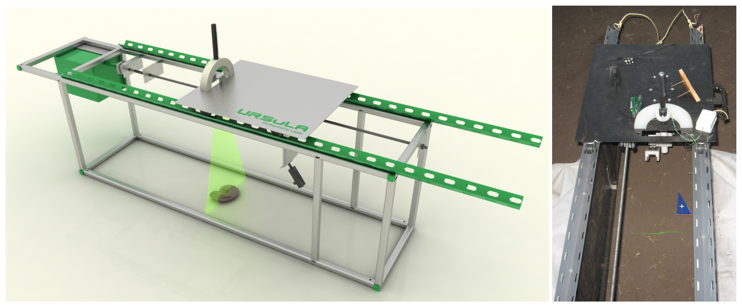
The laser unit for surface surveys (URSuLa) is a laser profiler which enables the measurement of soil roughness through 2-D digital modeling of the soil surface in an non-contact way. Figure 1 depicts an scheme of the laser profiler. It comprises a rectangular parallelepiped-shaped metal frame with two guides, over which a mobile, motor-driven platform is mounted. Attached to the platform there are a laser unit, a case containing an optical system and a small, commercial-grade camera (Logitech^® QuickCam pro for Notebooks), at fixed locations. The platform is placed at a distance of 30 cm over the frame base. The laser beam points downwards and is scattered by a cylindrical lens within the case to obtain a laser line of 25 cm length over the ground surface with a beam width of 1 mm. The camera points obliquely to the laser line in such a way that its field of view includes the whole line. Pictures are taken by the camera (2 MP resolution), which is placed 20 cm off the laser beam and 20 cm over the ground. The focal length of the camera is 3.7 mm and the ground sampling distance is 0.25 mm/pixel. Under this set-up, the laser line depicts a transect of the surface mimicking its shape, and it is stored as digital information through the camera.

Calibration is done following the method described in [19] to map pixel coordinates on the picture into millimeter coordinates over the ground. A transmission system coupled to the motor provides with longitudinal motion to the platform (see Figure 1), so as to obtain a 0.80 m by 0.25 m scannable area. Opaque panels (not shown) are attached around the metal frame to avoid the solar daylight diminishing the contrast of the laser beam onto the soil surface. The laser profiler is capable of measuring surface heights with an accuracy of 1 mm. In planimetry, the accuracy is 0.5 mm in the direction of the laser line and 1 mm in the direction along the frame. In the direction along the laser line, the accuracy is given by the distance between two contiguous pixels onto the laser line transformed into the millimeter-reference frame using the polynomial transformation from the calibration step. Along the frame, the accuracy of the measurements is given by the accuracy in controlling the motor-driven platform which carries the laser. The platform motion is finely controlled by a stepper motor, which is positioned with an accuracy of 1 mm. 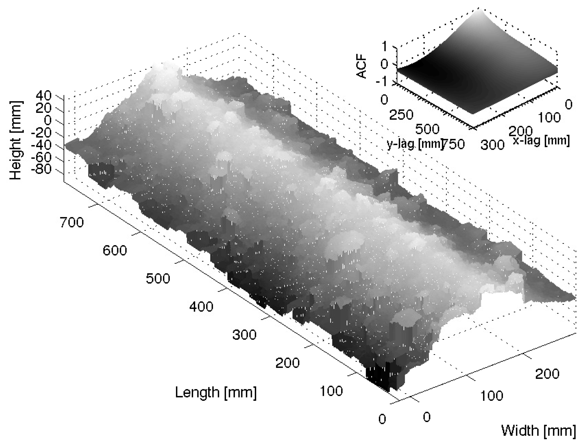Figure 2 shows a digitalization from a ploughed surface with a clear furrow.

As for the portability, URSuLa weighs approximately 15 kg and is easily handled by a two-man team. Approximately half of its weight is due to a long-lasting battery (17 ampere-hour) which can be replaced by a lighter one provided a replacement back-up battery is available in the field. The battery feds the electronics as well as an embedded PC used to operate the device and to store the data. Once the device is positioned onto the ground surface, one full scan takes ~1 min. Most of the time spent in the field is dedicated to move from one point to the next carrying the device.

The sequence of processing the digital record involves two major steps. Firstly, the soil transect is identified in every picture based on the high contrast of the laser line relative to the soil surface. The pixel coordinates of the laser line onto the picture are transformed into millimeter coordinates and then stored in a matrix as heights and positions. This step is repeated after the platform is placed 1 mm away from the preceding position and until the entire surface extent is profiled. Secondly, the surface is assembled by joining all the transects using their position information relative to the metal frame stored in every picture. A 3-D render of the surface is generated at a 1 mm by 1 mm sampling interval grid by a nearest-neighbor interpolation. The surface covers approximately a 0.80 m by 0.25 m soil patch. Shadowed points (i.e., points that are not visible from the camera point of view due to the blockage of another, more elevated point in-between) are interpolated using a nearest-neighbor algorithm as well. Once the entire surface is rendered at 1 mm by 1 mm grid size, about 250 lengthwise transects (one per millimeter) are computed. Each transect is detrended separately to remove the mean profile height and profile tilt, thus correcting for any instrument misalignment in the experimental set-up. Thus, these detrended transects are used as 1-D profile samples of the surface random component.

A small barrel distortion (i.e., lens effect which causes straight lines to curve out) were detected in the calibration procedure in laboratory. It was observed on the top of the pictures, where only would affect terrain features of around 20 cm height. For typical soil elements (0–10 cm height), this distortion does not have any influence on measurements. In field measurements, standing crop residue has a contrasting height with respect to the points over the soil surface. Thus, height points from crop elements are identified as outliers by comparing the height of their nearest neighbors over the soil. Before the second processing stage, these outliers are disregarded. The presence of laid crop residue is more difficult to deal with. The impact of laid crop residue is reduced by selecting sites with a relative low amount of crop elements. It might be necessary to remove some crop residues by hand prior to instrument deployment.

2.2. Instrument Limitations

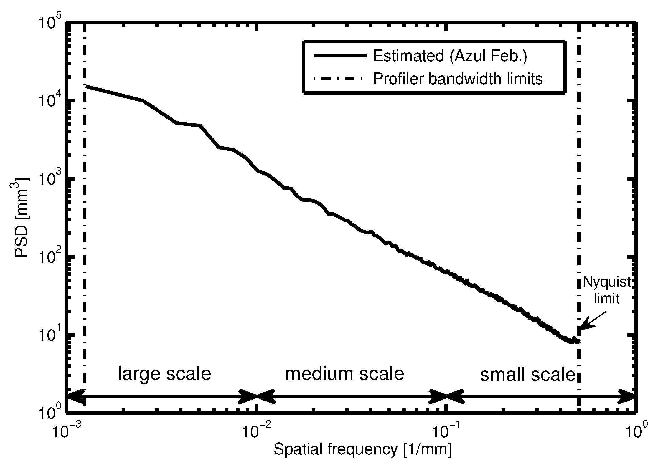
The limitations relative to both the finite dimensions and finite sampling interval of the measurement device can be analyzed by means of the power spectrum (i.e., the Fourier transform of the autocorrelation function) of the profile record. In effect, roughness measurements using profilers are always band-limited in the sense that they lay between a minimum $f_{min}=\frac{1}{L}$ and a maximum $f_{max}=\frac{1}{\Delta x}$ in the spatial frequency domain, being these determined by the profile length L and the sampling interval $\Delta x$, respectively. For URSuLa, $f_{min}=\frac{1.25\times {10}^{-3}}{\text{mm}}$ and $f_{max}=\frac{1}{\text{mm}}$, indicating the spatial frequency range of soil features which URSuLa is sensitive at.

Figure 3 depicts a power spectrum measured by URSuLa (profile length 800 mm and sampling interval 1 mm) corresponding to 10 single profiles averaged over the same field (Azul, February 2009; see Section 2.4). From this average power spectrum, it turns out that the estimation of the low-frequency components is better than the high-frequency ones (i.e., $f>\frac{1\times {10}^{-1}}{\text{mm}}$). This is due to the fact that low-frequency components are sampled at a larger density of points per frequency unit, since the sampling frequency URSuLa measures each roughness component in the soil profile is $\frac{1}{\Delta x}$. Yet, most of the shape of the small-scale spectrum is still captured by the laser profiler, constrained to the Nyquist sampling criterion $f<\frac{f_{max}}{2}$ [25]. Therefore, the laser profiler URSuLa is suited to estimate small-scale, random component roughness parameters s and l from 1-D profiles.

2.3. Roughness Descriptors

As mentioned in the Introduction, surface roughness conditions may be summarized using only two parameters derived from 1-D profiles: The surface height standard deviation s, defined for a discretized, detrended profile of n points as

$$s={\left[{\displaystyle \frac{1}{n-1}}\sum _{i=1}^n{\left(z\left(x_i\right)\right)}^2\right]}^{\frac{1}{2}}$$

(1)

where $z\left(x_i\right)$ is the height of the soil profile measured from the mean line at $x_i$, and the autocorrelation function ρ at ξ,

$$\rho \left(\xi \right)=\frac{{\sum }_{i=1}^{n}z\left(x_i\right)z(x_i+\xi )}{{\sum }_{i=1}^n{z}_i^2}$$

(2)

from which the correlation length l, defined as the distance so that $\rho \left(l\right)=\frac{1}{e}$, is computed. For stochastic surfaces, $\rho \left(\xi \right)$ approaches to 0 for ξ approaching to infinity, indicating that beyond a certain distance, two surface points become uncorrelated. Also, the definition in Equation (2) is normalized in such a way that $\rho \left(\xi \right)\to 1$ as $\xi \to 0$. The parameterization given in Equations (1) and (2) is only valid for the small-scale roughness. From each 3-D surface rendering, about 250 transects separated away one millimeter were used as 1-D profile samples. On each sample, s and l are computed and then averaged, leading to N = 83 pairs (s, l) for this paper.

2.4. Field Work

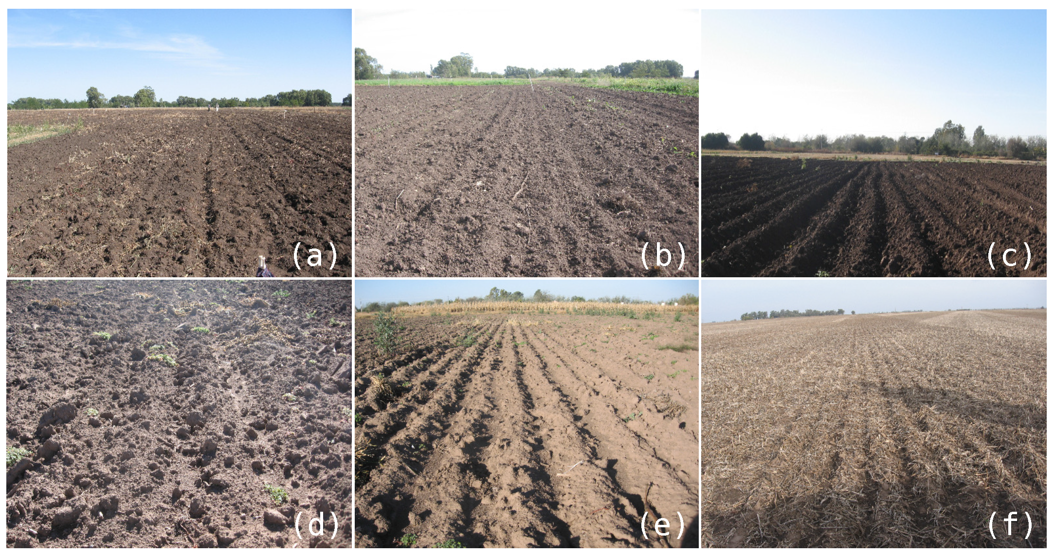
In order to obtain a sound statistical sample of roughness conditions and to diminish the dependence of the results on a particular site, an extensive campaign was performed over three sites spread out on the Argentine’s Pampas—vast plains extending westward across central Argentina from the Atlantic coast to the Andean foothills and one of the major agricultural regions in the world. The main characteristics of the different fields are given in

Table 1. Field sites description. N is number of parallel profile measurements.

Site Name	Date	Lat/Lon	Soil Texture ${}^1$	Management Practice	Tillage State (Type)	N
Azul	February 2009	36°49′38″S/	Lo/	Till (Test site)	Ploughed (moldboard)	16
	April 2009	59°53′17″W	SiLo		Ploughed (moldboard)	21
CETT	May 2011	31°31′17″S/	SiClLo	Till (Test site)	Ploughed (moldboard)	17
		64°27′06″W			Harrowed (double-acting disk)	19
Bell Ville	May 2011	32°40′26″S/	SiClLo	No-till (Private)	Seedbed (wheat)	10
		62°35′37″W

${}^1$ USDA classification: loam (Lo), silty loam (SiLo), silty clay loam (SiClLo).

. Azul site is managed by the National University of the Center of the Buenos Aires Province (UNICEN), CETT site belongs to the Argentine Space Agency (CONAE), whereas Bell Ville site belongs to a private farmer. Since Azul and CETT are test sites, the tillage management practice was experimentally set at the time the field work was done. In Bell Ville, management practice was exclusively decided by the owner. Azul site was visited twice in February and April (Azul F and Azul A) presenting ploughed (PLD) fields. CETT and Bell Ville were visited once, with three different tillages over several fields: ploughed and harrowed with disk (DSK) for CETT and seedbed (SBD) for Bell Ville. One of the CETT’s harrowed fields appeared clearly weathered (WTH) and was analyzed separately. In Table 1 the farming activities prior to measurements are also reported. In Azul site, the tillage operations were done the day before the measurements were taken. The tillage operations in CETT site were done the week before and there were no rain events during that week. Still, somewhat of wind erosion was observed from a visual inspection in one of the harrowed field. The seedbed field in Bell Ville was done using a no-till planter the week before the measurements were taken, with no rain events during that week. Figure 4 depicts the tillage conditions at the time the soil roughness measurements were done. Since tillage furrows were presented, only profiles parallel to tillage direction were used in this study.

2.5. Data Analysis

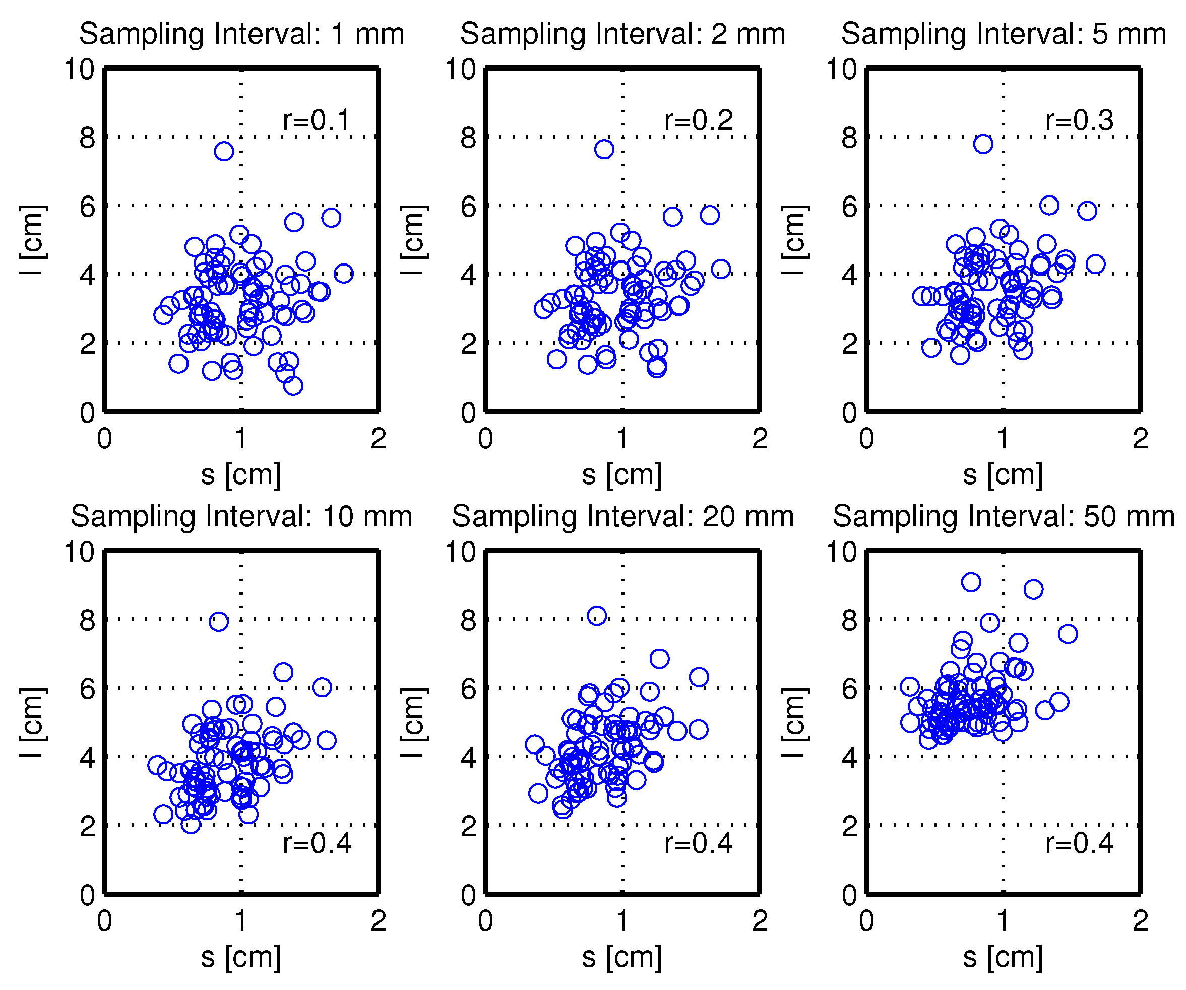
URSuLa is able to digitize a soil patch of 0.80 m by 0.25 m with the surface heights evenly sampled at a 1 mm by 1 mm grid size. This 3-D rendered surface is decomposed into 0.80 m-length transects which are detrended by a linear polynomial. Each detrended, lengthwise, 1-mm-sampling-interval transect is then undergone a moving average filter. In this process, a sequence of consecutive height points within a predefined window are averaged out and the resulting height is placed at the center position of the original sequence, thus synthesizing profiles at different sampling intervals according to the window length. Window lengths were chosen to span 2, 5, 10, 20 and 50 consecutive height points from 1-mm-sampling-interval profiles, thus mimicking profiles acquired by profiling techniques with different sampling intervals.

Once the processed profiles are at hand, roughness parameters height standard deviation s, autocorrelation function and correlation length l are computed and their dependence on the sampling interval are evaluated on a field basis (i.e., roughness parameters are averaged out within each field). Comparison of experimental ACF with theoretical Gaussian and exponential models is also done. 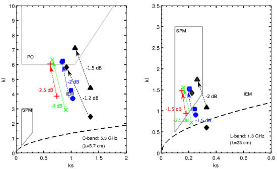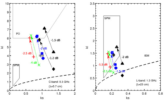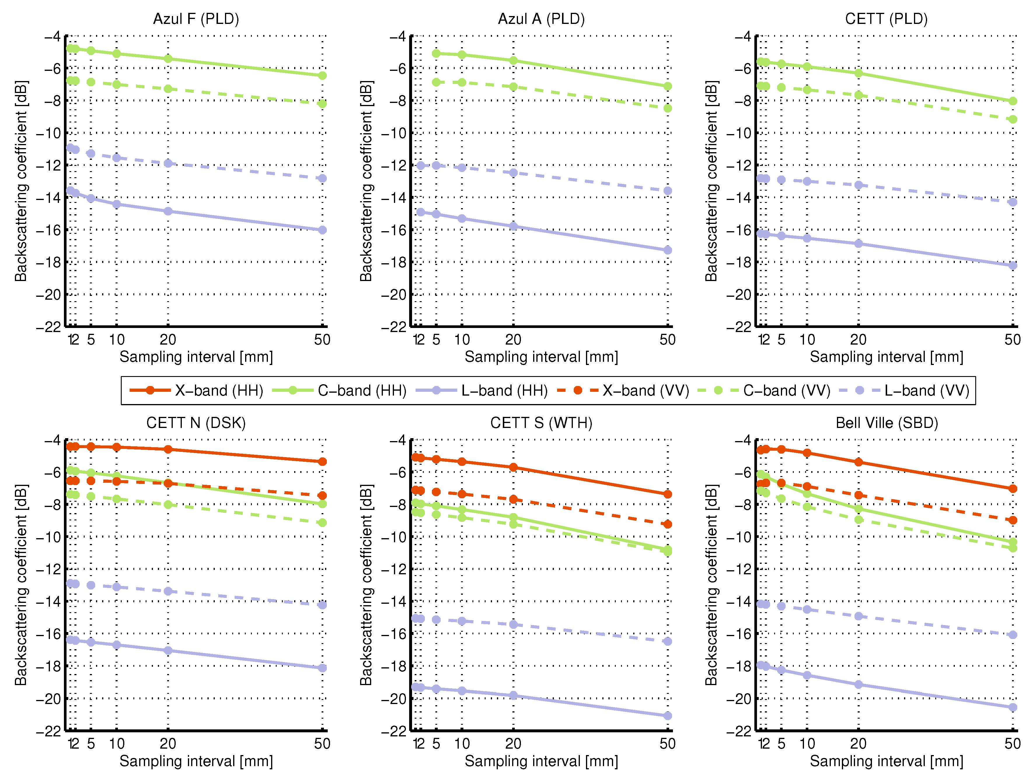Then, the impact of the different sampling intervals on the separability of the different tillage conditions is assessed onto a (s, l)-plane. Finally, a theoretical electromagnetic scattering model is employed to identify the spatial scales more relevant to accurately account for the microwave response of a soil surface. 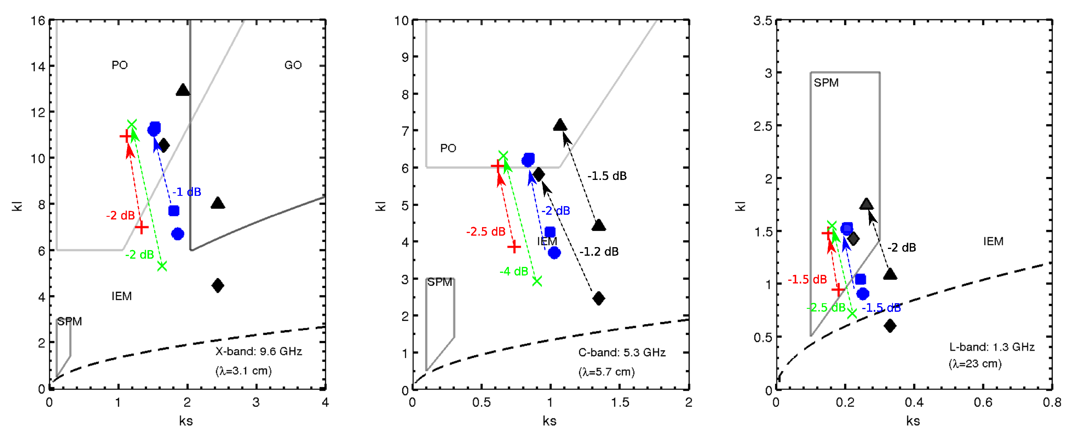This model, referred to as IEM2M [23,24], predicts co-polarized backscattering coefficients HH and VV from a random rough surface given its dielectric constant, roughness parameters and autocorrelation function, besides the observation geometry parameters frequency and beam incidence angle.

3. Results

3.1. Tillage-Induced Roughness

In agricultural soils, surface roughness is induced in tillage activities by a variety of implements used for different purposes. Roughly speaking, the disturbance of the soil is produced at both vertical and horizontal directions after a particular tillage implement passes. The subsequent shape, size and arrangement of the surface constituents determine the height standard deviation s and the correlation length l. To put this statement in a more quantitative way, Figure 5 depicts soil roughness as box plots for the sites described in Table 1. Roughness parameters s and l were computed from measurements along (parallel) tillage structure.

It is observed a dependency between s and tillage activities in such a way that the more intensive the soil disturbance, the larger the s values. In addition, weathering caused by wind erosion had smoothing effects on the soil roughness of field CETT S (WTH). The high variance corresponding to Bell Ville s values might be due to the presence of stubble that could not be completely removed without disturbing the soil surface (i.e., only loose stubble was removed). Regarding to the correlation length l, dependency on tillage was somewhat less marked.

3.2. Impact of Spatial Sampling Interval on Roughness Parameters s and l

Comparison among roughness parameters computed from the original 1-mm-sampling-interval profiles and from the profiles synthesized at the different sampling intervals is shown in Figure 6, where the field medians are plotted and error bars are represented by the 25th and the 75th percentiles. The decrease on s as sampling interval increased seemed quite expectable, because of the low-pass feature of the moving-average technique used to synthesize profiles at larger intervals. Conversely, correlation length increased as sampling interval increased due to the lack of high-frequency, small-scale features on the averaged profiles. In fact, since large-scale features could not be measured by URSuLa due to the lower band limit of its power spectrum, further averaging will lead to $s\to 0$ and $l\to \infty$.

Error bars presented a complex behavior for which some remained constant and other decreased as sampling interval increased. This is quite interesting, as it is contrary to the variation of the roughness parameters on profile length [8], where it was experimentally found that variation of s decreased as profile length increased. Conversely, variation of l seemed to increase as profile length increased [8]. Decreasing error bars are expected for increasing sampling intervals, since the profiles became similar to one another, which means that variability of the roughness parameters should be smaller. However, it should be noted that the measurements shown in Figure 6 are median values for s and l for each field (Azul, CETT, etc.), which means that N independent measurements within each field were taken into account (see Table 1). Here, the influence of the sampling interval on the variability of the median values was somewhat masked by the within-field variability. The smoothing effect of the low-pass filtering is noted on comparing each single profile, not in the field-median roughness estimate. Error bars remaining constant just indicates that the roughness features for these fields were soundly estimated from the profiles, mostly regardless of the sampling interval used to estimate them.

In Figure 7, the correlation length l as a function of the height standard deviation s for the sampling intervals 1, 2, 5, 10, 20 and 50 mm is shown. The Spearman rank-order correlation coefficient r [26] were computed to assess the statistical dependence between s and l. For the smaller sampling intervals, the correlation coefficient showed a low value due to the higher variance of the s and l estimates in comparison to larger sampling intervals. As the sampling interval increased, the correlation coefficient increased until $r=0.4$. A direct relationship between the height standard deviation s and the correlation length l was previously found in [12,27]. In [12] correlation coefficients r between 0.26 and 0.48 were reported for seedbed to ploughed fields for a sampling interval of 5 mm. In addition, in [27] it was found $r=0.56$ for seedbed and ploughed fields for a sampling interval of 20 mm. The results shown in Figure 7 are in accordance to these.

3.3. Autocorrelation Function

The impact of the small-scale component on the autocorrelation function is shown in Figure 8, where an overestimation of the correlation length l is clearly observed for increasing sampling intervals. This overestimation is higher for the smooth surface in Bell Ville (SBD) site than for the rough surface at Azul F (PLD). It is also clear that a steeper slope at the origin was found for the profile at 1-mm-sampling-interval than for the longer intervals, illustrating the loss of high-frequency roughness components as sampling interval increased, and in accordance with [16].

Theoretical descriptions of autocorrelation function ρ describing horizontal random roughness component are of the exponential ($\rho \left(\xi \right)=e^{-\frac{\xi }{l}}$) or Gaussian ($\rho \left(\xi \right)=e^{-\frac{{\xi }^2}{l^2}}$) type [28]. In Figure 9, overlapped to the experimental ACF (black line) are the theoretical exponential (blue line) and Gaussian (red line) ones, generated using the correlation length estimated from the experimental ACF. The experimental ACF was computed by averaging all the single ACFs within each tillage condition. The nominal 1-mm (Figure 9a) and the averaged 20-mm (Figure 9b) cases are shown for contrasting. At 1-mm-sampling-interval, exponential correlation function agreed better with experimental ACF than the Gaussian case for the medium roughness tillage states CETT (PLD), CETT N (DSK) and CETT S (WTH). Therefore, for these conditions, the small-scale components dominates the roughness features, well approximated with an exponential correlation function in agreement with [7]. For the rougher states Azul F (PLD) and Azul A (PLD), the small-scale roughness components were overestimated by the exponential and Gaussian types. Yet, the exponential type resembled more closely the experimental ACF. On the other hand, the large-scale roughness components (i.e., $lags>l$, where lag is the spatial shift at which the discrete autocorrelation function were computed) are better described by the exponential correlation function for all the tillage states. At 20-mm-sampling-interval, the exponential type correlated better with the experimental ACF for $lags<l$. For $lags>l$, the experimental ACF was slightly closer to the Gaussian, though.

3.4. Scatter Plots and Data Clustering

In Figure 10, (s, l) scatter plots for 1 mm, 5 mm and 20 mm sampling intervals are shown, where each point represents a field measurement (totaling N = 83). Corresponding covariance ellipses are computed at CL 80%, with the filled markers indicating the center of each cluster. For each sampling interval, the separability of the clusters (i.e., the relative distance among their centers) indicates the discrimination capabilities of the roughness descriptors on the different tillage implements employed on each field. A particular roughness category can be considered separated from the others when the center of any other cluster is sufficiently far apart from its own center, as compared to its bound. This statement can be put into a quantitative way by the following measure of separability $D_{i,j}$ among the clusters

$$D_{i,j}=\sqrt{S_{i,j}^2+L_{i,j}^2}$$

(3)

where $S_{i,j}$ and $L_{i,j}$ are separability measures of s and l for the i-th cluster compared with the j-th cluster, defined as

$$S_{i,j}={\displaystyle \frac{|s_i-s_j|}{std\left(s_i\right)+std\left(s_j\right)}}$$

(4)

$$L_{i,j}={\displaystyle \frac{|l_i-l_j|}{std\left(l_i\right)+std\left(l_j\right)}}$$

(5)

where $s_{i,j}$ and $l_{i,j}$ are the means and $std$ stands for the standard deviation. In Equations (4) and (5), the subscript indicates the j-th cluster which the given i-th cluster is compared with. These measures are shown in

Table 2. Measures of separability for the clusters at 1-mm-sampling-interval.

	Azul A (PLD)	CETT (PLD)	CETT N (DSK)	CETT S (WTH)	Bell Ville (SBD)
Azul F (PLD)	0.7357	0.7468	0.6497	1.5046	1.0034
Azul A (PLD)		0.8779	1.0019	1.5378	0.7666
CETT (PLD)			0.2933	0.9142	0.5183
CETT N (DSK)				0.6915	0.7119
CETT S (WTH)					0.6610

,

Table 3. Measures of separability for the clusters at 5-mm-sampling-interval.

	Azul A (PLD)	CETT (PLD)	CETT N (DSK)	CETT S (WTH)	Bell Ville (SBD)
Azul F (PLD)	0.7062	0.7441	0.5946	1.4597	1.0231
Azul A (PLD)		0.5301	0.6984	1.1753	0.6495
CETT (PLD)			0.2818	0.8816	0.6313
CETT N (DSK)				0.6743	0.5417
CETT S (WTH)					0.4035

and

Table 4. Measures of separability for the clusters at 20-mm-sampling-interval.

	Azul A (PLD)	CETT (PLD)	CETT N (DSK)	CETT S (WTH)	Bell Ville (SBD)
Azul F (PLD)	0.7301	0.7651	0.5701	1.4035	0.9897
Azul A (PLD)		0.2844	0.4827	0.8606	0.6221
CETT (PLD)			0.2663	0.8016	0.9020
CETT N (DSK)				0.6576	0.4023
CETT S (WTH)					0.1577

, for the sampling intervals corresponding to Figure 10.

For instance at 1-mm-sampling-interval (Table 2), the rougher categories Azul F (PLD) and Azul A (PLD) are well discriminated in relation with the smoother one CETT S (WTH) ($D>1.5$). Separability of Azul A was also marked for the medium-rough category such as CETT (PLD) and CETT N (DSK). Conversely, CETT (PLD) and CETT N (DSK) merged together to a single category. Azul F (PLD) showed a particular clustering in relation to its neighbors, since its center lay on the bounds of two different clusters, indicating it is some kind of intermediate category between the roughest one of Azul A (PLD) ($D=0.7357$) and the medium-rough category of CETT (PLD) ($D=0.7468$).

It is observed how the separability of the clusters became diffuse as the sampling interval increased to 5 mm (Table 3) and 20 mm (Table 4), leading to a poorer discrimination. This implies that there were roughness components, characteristic of each tillage state, only detectable at 1-mm and 5-mm-sampling-interval, and not at 20-mm-sampling-interval. In other words, soil aggregates varied among classes, thus affecting the small scale roughness and therefore the roughness parameters. Clustering enables to further the analysis by using the center of each cluster as an indicator of the mean tillage conditions found on each field.

3.5. Sampling-Interval-Dependent Roughness Parameters and Electromagnetic Scattering Models

For isotropic surfaces (when only random roughness is present) or when coherent effect due to row structure has no relevant contribution to surface scattering (i.e., for a suitable observation geometry), scattering response can be evaluated using theoretical models such as Small Perturbation Model (SPM), Physical Optics (PO), Geometrical Optics (GO), and Integral Equation Model (IEM), within their corresponding validity regions. Figure 11 depicts the interval-dependent cluster centers onto a $(ks,kl)$-plane ($k=\frac{2\pi }{\lambda }$) superimposed to the validity regions of the models computed for an incidence angle $\theta =40°$ and for three frequencies: 1.3 GHz (L-band), 5.3 GHz (C-band) and 9.6 GHz (X-band). See [29] for a summary of the validity conditions for SPM, PO and GO. The validity region for the IEM (dashed line) is computed from [28] for $\theta =40°$. Arrows indicate the variation in surface backscattering as evaluated from IEM2M [23,24] from 1-mm (tail) to 50-mm-sampling-interval (head) roughness. An incidence angle $\theta =40°$, a dielectric constant $\epsilon =20$ and a 2-D exponential correlation function were used to evaluate IEM2M. Values are an average for HH- and VV-polarizations, pointing out the sensitivity of the backscatter response to the small-scale components, only accurately provided by 1-mm-sampling-interval measurements. Figure 11 also indicates when limiting models (i.e., SPM, PO and GO) would provide a performance in predicting scattering response as accurate as the IEM without its computational requirements.

At X-band, roughness parameters had the larger span through the different validity regions in comparison to C- and L-band. However, the sensitivity of surface backscattering to small spectral components was somewhat slightly marked (1–2 dB). Surface scattering at X-band ($\lambda =3.1\text{cm}$) deserves special care, as it depends on the smaller components of the surface. According to the $\frac{\lambda }{10}$-rule of thumb, this implies a sampling interval $\Delta x<3\text{mm}$, which are close to the edge of the measurement capabilities of a millimeter-sampling-interval roughness measurement instrument. Yet, the roughness parameters measured at 1 mm sampling interval might even underestimate high-frequency components necessary for an accurate modeling at X-band. Moreover, for the rougher fields Azul F (PLD), Azul A (PLD) and CETT (PLD), the roughness parameters measured at different sampling intervals led to an un-physical backscatter response (no arrows), for which backscattering coefficients increased as the surface got smoother, as evaluated by IEM2M. For this reason, these three fields was disregarded in the next analysis at X-band.

Sensitivity to small spectral components was highly marked at C-band, where a dynamic range up to 4 dB were reached. In any case, the span of the roughness parameters was still broad. For longer wavelengths such as those of L-band ($\lambda =23\text{cm}$), the roughest field (black diamond) fell outside IEM validity region for 1-mm-sampling-interval measurements. The use of SPM is also allowed for the large sampling interval measurements. In this case, a moderate sensitivity of about 1.5–2.5 dB were reached. Overall, note that roughness parameters computed from 50-mm-sampling-interval profile will lead to an underestimation on the backscatter response. This effect was less significant as the frequency decreased from C-band to L-band, indicating the loss of sensitivity of the scattering on the smaller components of the surface. For the smoother surfaces, backscatter response were well modeled by IEM or its limiting cases PO and SPM [23].

The question as to whether the $\frac{\lambda }{10}$-rule of thumb is a fair condition then arises. To contribute to its answer, a further simulation study was performed where the dependence of simulated backscattering coefficients on sampling-dependent roughness parameters were evaluated using IEM2M, as shown by Figure 12. For instance, at C-band, a significant underestimation of −4.2 dB between the roughness parameters at 1 mm and 50 mm sampling interval was observed on the HH polarization for Bell Ville (SBD). The rougher fields at Azul F (PLD) and Azul A (PLD) were moderately underestimated by −1.7 dB and 2 dB, respectively. VV polarization was less underestimated than HH, indicating that VV polarization was less sensitive to roughness. At L-band, an underestimation of −2.5 dB was observed on the HH polarization for the roughest field Azul F (PLD). CETT N (DSK) and CETT S (WTH) sites were moderately underestimated by −1.8 dB. It is also found that VV polarization was less underestimated than HH one. From this analysis it is clear that an underestimation of the small-scale roughness components, such that from a coarse sampling interval, will have a stronger negative influence at C-band than at L-band.

Moreover, it is also possible to retrieve the sampling interval for which simulated backscatter responses are within some threshold (e.g., 1.0 dB) with respect to the ones computed at the smallest sampling interval $\Delta x=1\mathrm{mm}$. For instance, simulated backscatter responses are within 1.0 dB with respect to the 1-mm-sampling-interval roughness parameters provided $\Delta x<5\mathrm{mm}$ at C-band and $\Delta x<15\text{mm}$ at L-band. In other words, it turns out that roughness components of about ~$\frac{\lambda }{10}$ have a dominant contribution to scattering. From the above discussion, to get an accurate enough scattering prediction (error within 1.0 dB) from the electromagnetic models and for the variety of tilled surfaces analyzed here, the following linkage between the working wavelength and the sampling interval might be established:

• C-band (λ = 5.7 cm) → $\Delta x\le 5\text{mm}$,
• L-band (λ = 23 cm) → $\Delta x\le 15\text{mm}$.

Thus, the sampling intervals listed can be regarded as the larger sampling interval allowed to characterize soil surfaces in order to accurately model (i.e., within 1 dB) their microwave backscatter response.

4. Discussion

Microwave backscatter response from agricultural surfaces depends on the arrangement and shape of the surface constituents at several spatial scales. When no coherent effect is observed, the random component of the surface roughness has the dominant contribution to the microwave response. The random component of surface soil roughness is estimated from 1-D profiles using two parameters that accounts for the vertical (s) and horizontal (l) roughness component. Non-contact profiling techniques such as laser triangulation, laser scanning or photogrammetry deal with a number of different sampling intervals, due to the diversity of experimental set-ups and to the technique itself.

The enhanced technical capabilities of URSuLa (i.e., 1 mm sampling interval, an extended profiling area and multisite capability) enables an experimental study aimed to improve the understanding of the spatial scales involved in microwave backscattering of soil surfaces under different tillages. Within this context, the effect of sampling-interval-dependent roughness parameters on backscatter response at X-, C- and L-band was assessed through an experimental study of the dependence of the roughness descriptors on the sampling interval. Sampling intervals range from large (50 mm) to small (1 mm), with intermediate 20 mm, 10 mm, 5 mm and 2 mm intervals, thus covering a large number of profiling techniques. Large- and intermediate-sampling-interval profiles were synthetically derived from nominal, 1 mm ones and used to assess the variations of roughness parameters (s and l) depending on the sampling interval and their influence in soil surface backscatter response.

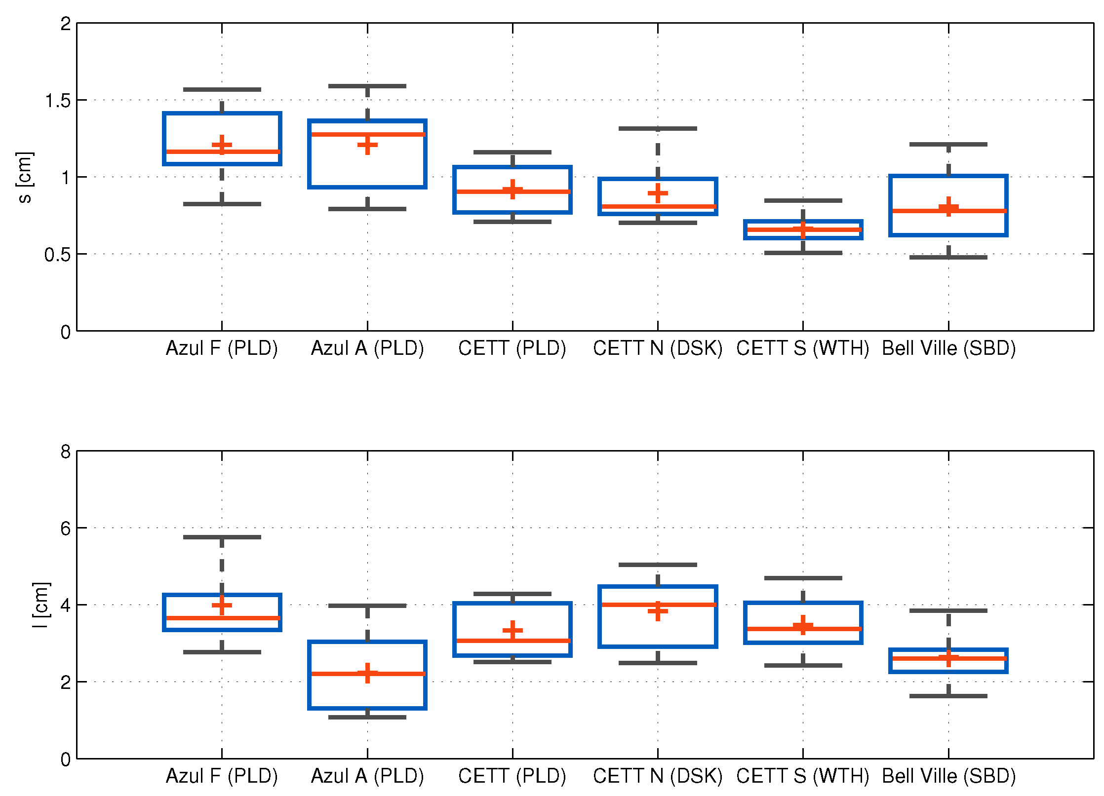
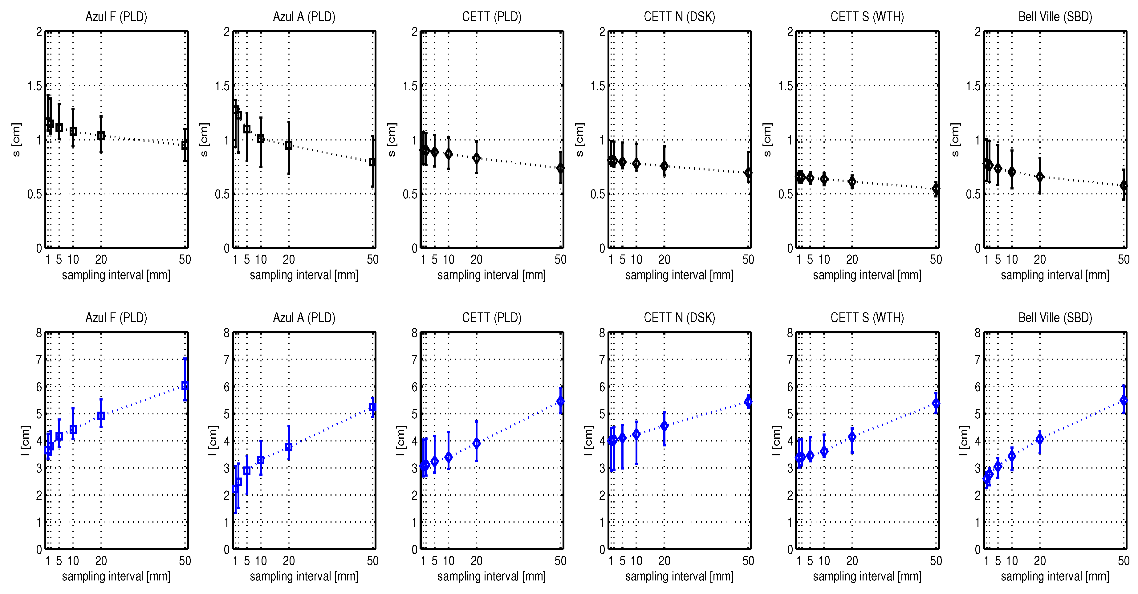
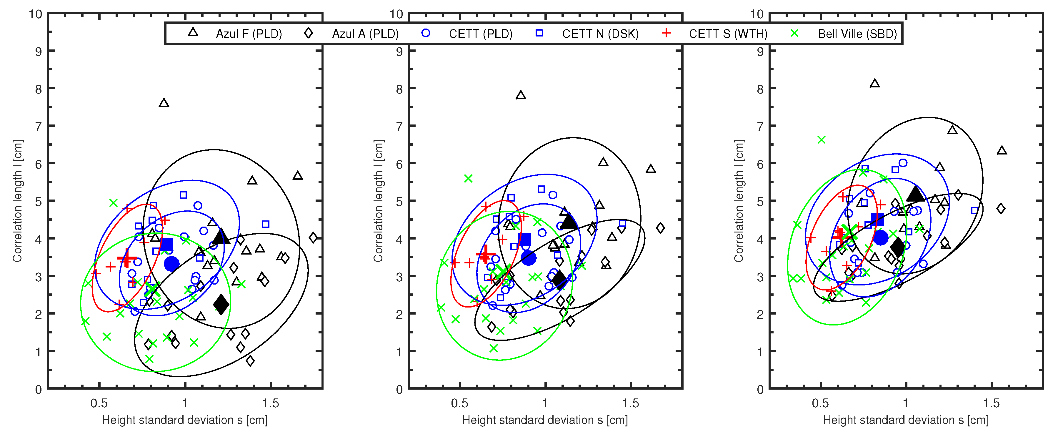
It was observed a dependency between s and tillage activities in such a way that the more intensive the soil disturbance, the larger the s values, in accordance to [7,8,12,30]. Regarding to the correlation length l, dependency on tillage was somewhat less marked, possible due to the limited profile length of URSuLa in comparison to other profilers [8]. In general, for the field medians, it was observed that the s values decreased and the l values increased as the sampling interval became coarser from 1 mm to 50 mm, which is a consequence of the smoothing effect of the low-pass filtering and of the finite lower band limit of URSuLa’s power spectrum. This led to less separable tillage classes in the sense of separability among clusters’ centers at coarse sampling intervals. Thus, it was highlighted the need for accurate measurements of the small scale components for discriminating among different tillage states. Also, it turned out that the uncertainties of these medians (i.e., error bars in Figure 6) are related to the variability within the fields, masking the influence of the different sampling intervals used. A direct relationship between s and l was found, where the results were in accordance to [12] for a sampling interval of 5 mm and to [27] for a sampling interval of 20 mm.

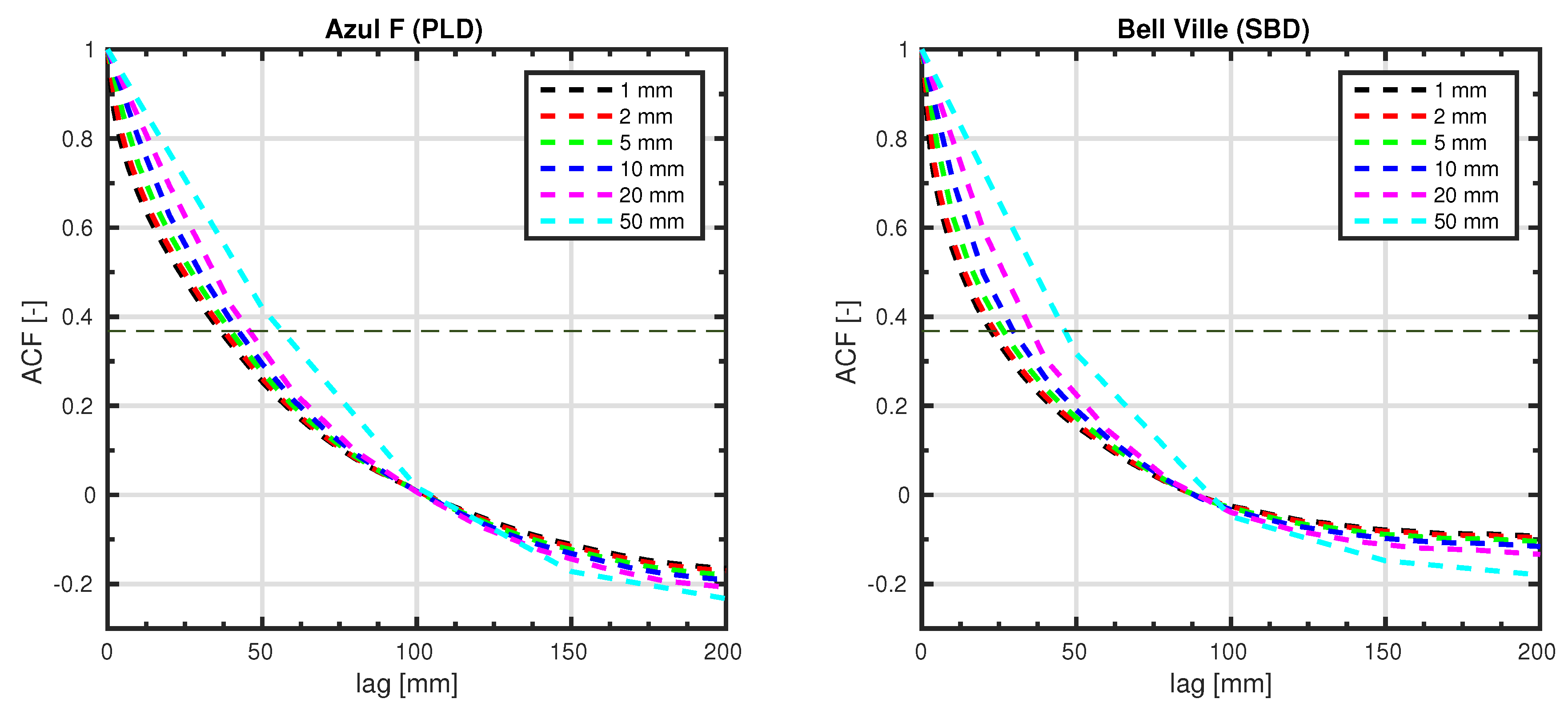
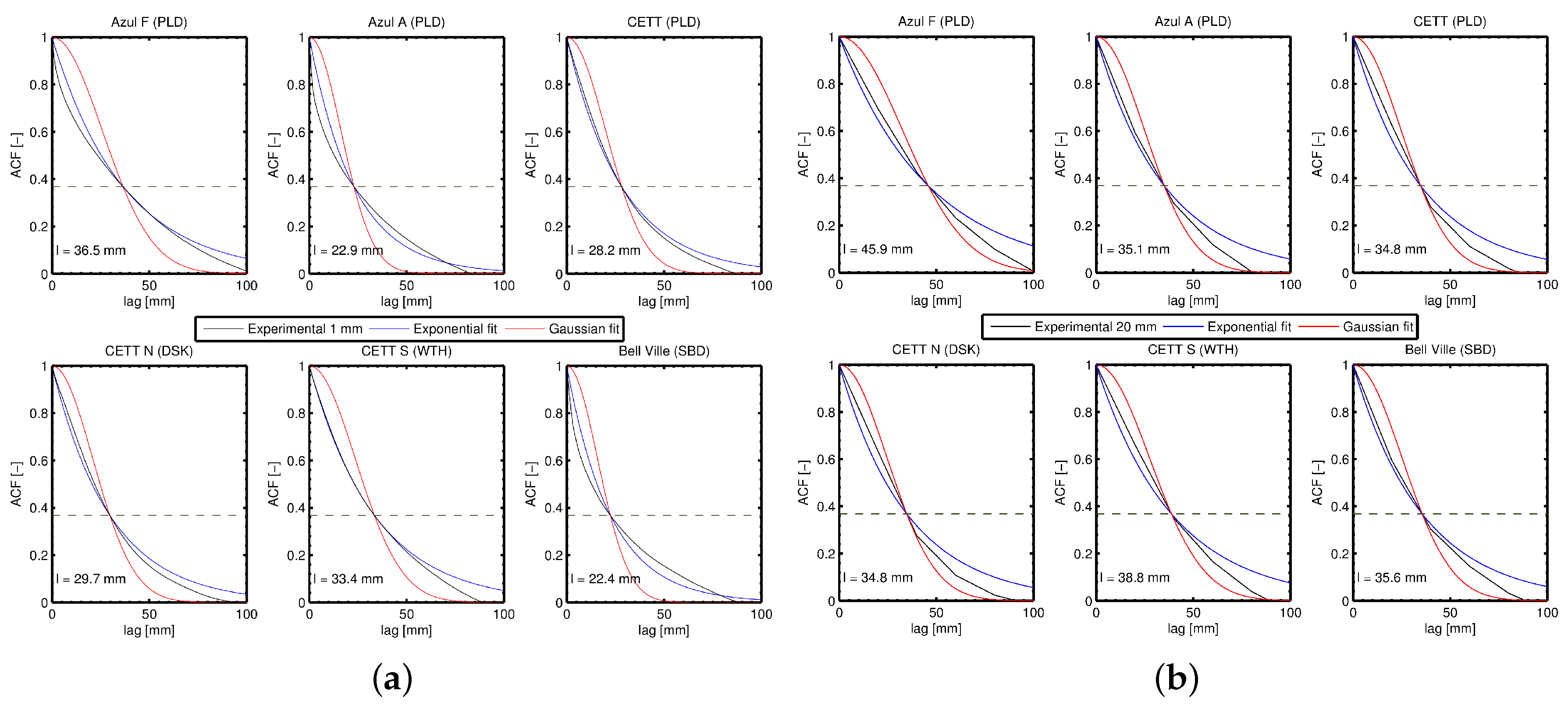
Regarding the ACF, the exponential ACF is characterized by smaller correlations at small lags compared to the Gaussian one. This causes that exponential ACFs to better describe the small-scale roughness in the profile than Gaussian ACFs [16]. Thus, the loss of high-frequency roughness component as the sampling interval increased led to an overestimation of the correlation length l, where the effect was more marked for the smooth roughness fields. Moreover, the small-scale components dominated the autocorrelation function for the medium roughness tillage states, where exponential correlation function agreed better with experimental ACF than the Gaussian case, with a poor agreement for the rougher fields nonetheless. This result is aligned with different studies in [6,7,8,16] that found the ACF was well approximated by exponential correlation function. For larger sampling intervals, a mixed behavior is observed, where the exponential type resembled more closely the experimental ACF for lags less than l but the Gaussian type was slightly closer for lags greater than l. Deviation from the exponential ACF especially at higher lags was also found in [20]. Since exponential and Gaussian theoretical descriptions do not always describe the roughness of natural surfaces very well, more complex models for ACF can be found in [31], where two analytical models introducing a varying power for the correlation function are suggested to fit the experimental ACF. Their shapes lie between the exponential and Gaussian cases, covering both types of ACFs, which might be useful for describing the intermediate shapes found in the 20-mm-sampling-interval ACFs. In view of the lack of similar studies systematically applied on real agricultural lands, the results presented here regarding the effect of the sampling interval can be combined to those describing the dependence of roughness parameters on profile length [8], to contribute to a better understanding on the scaling issues of the roughness and its complex nature.

Simulations carried out by using the theoretical backscatter model IEM2M demonstrated that this effect depended on the working wavelength and that coarsely-sampled roughness parameters will lead to larger error at short wavelengths such as C-band than at larger ones such as L-band. These errors come from an underestimation of the high-frequency components presented in the smaller scales. For the three bands studied here, an underestimation of the backscattering coefficient of about 1–4 dB was observed at coarser sampling intervals. It was also found that $\frac{\lambda }{10}$ could serve as an appropriate proxy to accounting for the relevant roughness components in the microwave backscattering response of soil surfaces. Selection of the profiling technique should rely on accurately characterize this surface component.

5. Conclusions

For a number of Remote Sensing applications, such as near-surface soil moisture retrieval, the contribution of soil roughness to the microwave backscatter of agricultural surfaces needs to be accurately quantified. Because of the increasing efforts towards that purpose, several profiling techniques are available to characterize surface roughness at different sampling intervals. With these data, the effect of sampling-interval-dependent roughness paramIn this paper, we contributed to answering the question of which sampling interval the profiles needed to be measured at to accurately account for the microwave response of agricultural surfaces. For this purpose, a custom-made, small-sampling-interval laser profiler was built and used to measure surface soil roughness over several agricultural sites in Pampas Plain, Argentina. eters on backscatter response was assessed through an experimental study of the dependence of the roughness descriptors on the sampling interval. A number of intermediate-sampling-interval profiles were synthetically derived from nominal, small-sampling-interval ones and used to assess the variations of roughness parameters depending on the sampling interval and their influence in soil surface backscatter response. The experimental and numerical results presented in this study demonstrated that roughness components of about ~$\frac{\lambda }{10}$ have a dominant contribution to C- and L-band microwave scattering. For some predefined tolerance with regards to backscattering coefficients, the results drawn by this work enables to select the more suitable profiling technique (for instance, the most affordable one which meets the sampling interval constraint) depending on the working wavelength. At X-band, a more detailed study on the electromagnetic scattering properties of soil surfaces is needed. A major conclusion drawn by this analysis is that to attain an accuracy of 1 dB, the sampling interval of the profiling technique should be less than 5 mm at C-band ($\lambda =5.7\mathrm{cm}$) and less than 15 mm at L-band ($\lambda =23\mathrm{cm}$). The results in this paper are intended to contribute to the rationale behind simulation studies and field experiments whose ultimate goal are to understand the microwave response of soil surfaces.

References

1. Zheng, B.; Campbell, J.; Serbin, G.; Galbraith, J. Remote sensing of crop residue and tillage practices: Present capabilities and future prospects. Soil Tillage Res. 2014, 138, 26–34. [Google Scholar] [CrossRef]
2. Dierking, W. Quantitative roughness characterization of geological surfaces and implications for radar signature analysis. IEEE Trans. Geosci. Remote Sens. 1999, 37, 2397–2412. [Google Scholar] [CrossRef] [Green Version]
3. Ulaby, F.T.; Moore, R.K.; Fung, A.K. Radar Remote Sensing and Surface Scattering and Emission Theory. In Microwave Remote Sensing: Active and Passive.; Addison-Wesley: Reading, MA, USA, 1982; Volume 2. [Google Scholar]
4. Beaudoin, A.; Le Toan, T.; Gwyn, Q. SAR observations and modeling of the C-band backscatter variability due to multiscale geometry and soil moisture. IEEE Trans. Geosci. Remote Sens. 1990, 28, 886–895. [Google Scholar] [CrossRef]
5. Shin, R.T.; Kong, J.A. Scattering of electromagnetic waves from a randomly perturbed quasiperiodic surface. J. Appl. Phys. 1984, 56, 10–21. [Google Scholar] [CrossRef]
6. Oh, Y.; Kay, Y.C. Condition for precise measurement of soil roughness. IEEE Trans. Geosci. Remote Sens. 1998, 36, 691–696. [Google Scholar]
7. Davidson, M.W.J.; Toan, T.L.; Mattia, F.; Satalino, G.; Manninen, T.; Borgeaud, M. On the characterization of agricultural soil roughness for radar remote sensing studies. IEEE Trans. Geosci. Remote Sens. 2000, 38, 630–640. [Google Scholar] [CrossRef]
8. Callens, M.; Verhoest, N.E.C.; Davidson, M.W.J. Parameterization of tillage-induced single-scale soil roughness from 4-m profiles. IEEE Trans. Geosci. Remote Sens. 2006, 44, 878–888. [Google Scholar] [CrossRef]
9. Alvarez-Mozos, J.; Casali, J.; Gonzalez-Audicana, M.; Verhoest, N. Assessment of the operational applicability of RADARSAT-1 data for surface soil moisture estimation. IEEE Trans. Geosci. Remote Sens. 2006, 44, 913–924. [Google Scholar] [CrossRef]
10. Baghdadi, N.; Cresson, R.; Pottier, E.; Aubert, M.; Zribi, M.; Jacome, A.; Benabdallah, S. A potential use for the C-band polarimetric SAR parameters to characterize the soil surface over bare agriculture fields. IEEE Trans. Geosci. Remote Sens. 2012, 50, 3844–3858. [Google Scholar] [CrossRef] [Green Version]
11. Zribi, M.; Chahbi, A.; Shabou, M.; Lili-Chabaane, Z.; Duchemin, B.; Baghdadi, N.; Amri, R.; Chehbouni, A. Soil surface moisture estimation over a semi-arid region using ENVISAT ASAR radar data for soil evaporation evaluation. Hydrol. Earth Syst. Sci. 2011, 15, 345–358. [Google Scholar] [CrossRef] [Green Version]
12. Davidson, M.W.J.; Mattia, F.; Satalino, G.; Verhoest, N.; Le Toan, T.; Borgeaud, M.; Louis, J.; Attema, E. Joint statistical properties of RMS height and correlation length derived from multisite 1-m roughness measurements. IEEE Trans. Geosci. Remote Sens. 2003, 41, 1651–1658. [Google Scholar] [CrossRef]
13. Magagi, R.; Berg, A.; Goita, K.; Belair, S.; Jackson, T.; Toth, B.; Walker, A.; McNairn, H.; O’Neill, P.; Moghaddam, M.; et al. Canadian experiment for soil moisture in 2010 (CanEx-SM10): Overview and preliminary Results. IEEE Trans. Geosci. Remote Sens. 2013, 51, 347–363. [Google Scholar] [CrossRef]
14. McNairn, H.; Jackson, T.; Wiseman, G.; Belair, S.; Berg, A.; Bullock, P.; Colliander, A.; Cosh, M.; bum Kim, S.; Magagi, R.; et al. The soil moisture active passive validation experiment 2012 (SMAPVEX12): Prelaunch calibration and validation of the SMAP soil moisture algorithms. IEEE Trans. Geosci. Remote Sens. 2015, 53, 2784–2801. [Google Scholar] [CrossRef]
15. Heald, M.A.; Marion, J.B. (Eds.) Classical Electromagnetic Radiation, 2nd ed.; Academic Press: New York, NY, USA, 1980.
16. Ogilvy, J.A.; Foster, J.R. Rough surfaces: Gaussian or exponential statistics? J. Phys. D Appl. Phys. 1989, 22, 1243. [Google Scholar] [CrossRef]
17. Milenkovic, M.; Pfeifer, N.; Glira, P. Applying terrestrial laser scanning for soil surface roughness assessment. Remote Sens. 2015, 7, 2007–2045. [Google Scholar] [CrossRef]
18. Verhoest, N.E.C.; Lievens, H.; Wagner, W.; Alvarez-Mozos, J.; Moran, M.S.; Mattia, F. On the soil roughness parameterization problem in soil moisture retrieval of bare surfaces from synthetic aperture radar. Sensors 2008, 8, 4213–4248. [Google Scholar] [CrossRef]
19. Darboux, F.; Huang, C. An instantaneous-profile laser scanner to measure soil surface microtopography. Soil Sci. Soc. Am. J. 2003, 67, 92–99. [Google Scholar] [CrossRef]
20. Zhixiong, L.; Nan, C.; Perdok, U.D.; Hoogmoed, W.B. Characterisation of soil profile roughness. Biosyst. Eng. 2005, 91, 369–377. [Google Scholar] [CrossRef]
21. Marzahn, P.; Rieke-Zapp, D.; Ludwig, R. Assessment of soil surface roughness statistics for microwave remote sensing applications using a simple photogrammetric acquisition system. ISPRS J. Photogramm. Remote Sens. 2012, 72, 80–89. [Google Scholar] [CrossRef]
22. Snapir, B.; Hobbs, S.; Waine, T. Roughness measurements over an agricultural soil surface with structure from motion. J. Photogramm. Remote Sens. 2014, 96, 210–223. [Google Scholar] [CrossRef]
23. Álvarez-Pérez, J.L. An extension of the IEM/IEMM surface scattering model. Waves Random Media 2001, 11, 307–329. [Google Scholar] [CrossRef]
24. Álvarez-Pérez, J.L. The IEM2M rough-surface scattering model for complex-permittivity scattering media. Waves Random Complex Media 2012, 22, 207–233. [Google Scholar] [CrossRef]
25. MacKay, D.J.C. Information Theory, Inference, and Learning Algorithms; Cambridge University Press: Cambridge, UK, 2003. [Google Scholar]
26. Press, W.H.; Teukolsky, S.A.; Vetterling, W.T.; Flannery, B.P. Numerical Recipes in C: The Art of Scientific Computing, 2nd ed.; Cambridge University Press: Cambridge, UK, 1992. [Google Scholar]
27. Baghdadi, N.; Zribi, M.; Loumagne, C.; Ansart, P.; Anguela, T.P. Analysis of TerraSAR-X data and their sensitivity to soil surface parameters over bare agricultural fields. Remote Sens. Environ. 2008, 112, 4370–4379. [Google Scholar] [CrossRef]
28. Fung, A.K. Microwave Scattering and Emission Models and Their Applications; The Artech House Remote Sensing library, Artech House: Norwood, Massachusetts, 1994. [Google Scholar]
29. Engman, E.T.; Wang, J.R. Evaluating roughness models of radar backscatter. IEEE Trans. Geosci. Remote Sens. 1987, 25, 709–713. [Google Scholar] [CrossRef]
30. Álvarez-Mozos, J.; Verhoest, N.E.; Larrañaga, A.; Casalí, J.; González-Audícana, M. Influence of surface roughness spatial variability and temporal dynamics on the retrieval of soil moisture from SAR observations. Sensors 2009, 9, 463–489. [Google Scholar] [CrossRef] [PubMed] [Green Version]
31. Zribi, M.; Baghdadi, N.; Holah, N.; Fafin, O. New methodology for soil surface moisture estimation and its application to ENVISAT-ASAR multi-incidence data inversion. Remote Sens. Environ. 2005, 96, 485–496. [Google Scholar] [CrossRef]
Figure 1. URSuLa (Unidad de Relevamiento de Superficies Laser—Laser unit for surface surveys) is a laser profiler capable of digitizing 2-D surfaces at a 1-mm-sampling-interval with an accuracy of 1 mm in height. In the illustration (left), a test object is placed to show the working principle of the instrument; A picture of the instrument deployed in the field (right).
Remotesensing 08 00458 g001
Figure 2. Sample agricultural soil surface measured over a field by URSuLa at a 1-mm- sampling-interval. Acquisition was parallel to the tillage direction over a ploughed field. ACF is also shown.
Remotesensing 08 00458 g002
Figure 3. Sample power spectrum for a 10-profile average measurement at Azul site. The range of the soil roughness scales are indicated as well as the bandwidth of the laser device.
Remotesensing 08 00458 g003
Figure 4. Illustration of the fields considered in this paper. On the top panel: (a) Azul in February 2009 (ploughed, PLD); (b) Azul in April 2009 (PLD); (c) CETT (PLD); On the lower panel: (d) CETT (disk-harrowed, DSK); (e) CETT (weathered, WTH); and (f) Bell Ville (seedbed, SBD). Several different tillage states are readily evident (see Table 1).
Remotesensing 08 00458 g004
Figure 5. Box plots for standard deviation s (upper panel) and for correlation length l (lower panel) as a function of the tillages found for the fields in Table 1. Measurements are taken along the tillage structure. On each box, the bar is the median, the “+” marker is the mean, the edges of the box are the 25th and 75th percentiles, the whiskers extend to the most extreme data points not considered outliers, and outliers (outside 99.3% coverage for data normally distributed) are plotted individually.
Remotesensing 08 00458 g005
Figure 6. Field medians (50th percentile) for height standard deviation s (upper panel) and correlation length l (lower panel) as a function of the sampling interval for the fields in Table 1. Direction of the measurements is along the tillage structure. Error bars are represented by the 25th and the 75th percentiles.
Remotesensing 08 00458 g006
Figure 7. Height standard deviation s versus correlation length l for the sampling intervals 1, 2, 5, 10, 20 and 50 mm. Spearman rank-order correlation coefficient r is shown as a measure of statistical dependence.
Remotesensing 08 00458 g007
Figure 8. Experimental autocorrelation function for different sampling interval for two contrasting fields: ploughed (left) and seedbed (right). Changes in the slope at origin are clearly observed.
Remotesensing 08 00458 g008
Figure 9. Experimental and theoretical correlation functions. Experimental correlation function is computed by averaging each one on a field basis. Theoretical correlation functions are exponential and Gaussian. (a) 1 mm sampling interval; (b) 20 mm sampling interval.
Remotesensing 08 00458 g009
Figure 10. Covariance ellipses (CL 80%) showing the clustering of roughness parameters for 1 mm sampling interval (left), 5 mm sampling interval (center) and 20 mm sampling interval (right). Filled markers indicate the centers of each cluster.
Remotesensing 08 00458 g010
Figure 11. Validity region for θ = 40 ° of the classical models Small Perturbation Model (SPM), Geometrical Optics (GO), Physical Optics (PO), and Integral Equation Model (IEM) onto a normalized roughness ( k s and k l ) plane for X- (left), C- (center) and L-bands (right). Arrows indicate the difference in backscattering coefficients as computed from IEM2M at 1-mm (tail) and 50-mm-sampling-interval roughness parameters (head). Model parameters are: incidence angle θ = 40 ° , dielectric constant ε = 20 and 2-D exponential correlation function. Markers are the same as in Figure 10.
Remotesensing 08 00458 g011
Figure 12. Simulated backscattering coefficients for sampling-interval-dependent roughness parameters s and l: Azul F (PLD), Azul A (PLD) and CETT (PLD) (upper panel); CETT N (DSK), CETT S (WTH) and Bell Ville (SBD) (lower panel). Model parameters are the same as in Figure 11. Missing points in Azul F (PLD) and CETT (PLD) led to un-physical backscatter response, Azul A (PLD) were outside IEM2M validity region.
Remotesensing 08 00458 g012