Estimation of Water Quality Parameters in Lake Erie from MERIS Using Linear Mixed Effect Models

Abstract

Linear Mixed Effect (LME) models are applied to the CoastColour atmospherically-corrected Medium Resolution Imaging Spectrometer (MERIS) reflectance, L2R full resolution product, to derive chlorophyll-a (chl-a) concentration and Secchi disk depth (SDD) in Lake Erie, which is considered as a Case II water (i.e., turbid and productive). A LME model considers the correlation that exists in the field measurements which have been performed repeatedly in space and time. In this study, models are developed based on the relation between the logarithmic scale of the water quality parameters and band ratios: B07:665 nm to B09:708.75 nm for log₁₀chl-a and B06:620 nm to B04:510 nm for log₁₀SDD. Cross validation is performed on the models. The results show good performance of the models, with Root Mean Square Errors (RMSE) and Mean Bias Errors (MBE) of 0.31 and 0.018 for log₁₀chl-a, and 0.19 and 0.006 for log₁₀SDD, respectively. The models are then applied to a time series of MERIS images acquired over Lake Erie from 2004–2012 to investigate the spatial and temporal variations of the water quality parameters. Produced maps reveal distinct monthly patterns for different regions of Lake Erie that are in agreement with known biogeochemical properties of the lake. The Detroit River and Maumee River carry sediments and nutrients to the shallow western basin. Hence, the shallow western basin of Lake Erie experiences the most intense algal blooms and the highest turbidity compared to the other sections of the lake. Maumee Bay, Sandusky Bay, Rondeau Bay and Long Point Bay are estimated to have prolonged intense algal bloom.

1. Introduction

Lake Erie, a turbid and regionally eutrophic lake, is the most southern and shallowest of the Laurentian Great Lakes. Total suspended matters (TSM) are a major contributor to the lake’s low water clarity [1]. The problem of excess nutrients and resulting algal blooms are also threatening the ecosystem of the lake and the economic activities of the surrounding regions. The ecological state of Lake Erie significantly affects its role as a natural, social, and economic resource, considering that the lake is as an essential drinking water source that also offers many opportunities for recreational activities, fisheries and tourism. As a result, the Lakewide Management Plan was signed in 1972 to restore and maintain the ecological health of the lake [2]. Ongoing efforts to support this plan require high-resolution measurements of the water quality parameters on a variety of spatial and temporal scales. Conventional field-based measurements of these parameters can be expensive and they are often sparse in either space or time, or both. Remote sensing has the potential to infer the lake bio-optical/water quality parameters, overcoming these concerns.

The emerging water radiance measured by remote sensing instruments depends on the water itself and its constituents. The water constituents interact with light and modify the incoming and outgoing radiation at various wavelengths. Therefore, remote sensing measurements of water leaving radiance can be related to the composition and concentration of water constituents. In Case I waters, chl-a concentration (phytoplankton population) and its co-varying particles are dominating the optical properties, which is the case in nearly all open ocean waters. However, optically complex inland waters and coastal waters are referred to as Case II waters, where chl-a alone is a poor predictor of light attenuation, and variations in TSM and colored dissolved organic matter (CDOM) are also important in light scattering or absorption, and therefore the water leaving radiance [3].

The delivery of data on water color has been explored using satellite sensors such as Landsat Thematic Mapper (TM)/Enhanced Thematic Mapper (ETM+) due to their relatively high spatial resolution of 30 m [4,5,6]. However, the shortcomings of Landsat in other capacities, such as its relatively low temporal resolution (i.e., 16 days), spectral and radiometric sensitivity, make the use of MODIS (Moderate-resolution Imaging Spectroradiometer) and MERIS (Medium Resolution Imaging Spectrometer) data more attractive for water quality monitoring [7,8,9]. Images from these satellite sensors compensate for the limitations of Landsat at the expense of a lower spatial resolution (ca. 250–500 m). MERIS was originally designed for water quality monitoring applications. Therefore, compared to MODIS, it has a more suitable spectral resolution in the red and near-infrared (NIR) to derive the secondary chlorophyll-a (chl-a) absorption maximum [10]. This is essential for Case II waters, as is the case for Lake Erie, where chl-a is not the predominant color-producing agent (CPA) and multiple non-covarying CPAs may also confound the reflectance signal, particularly at shorter wavelengths. Hence, the traditional and empirical blue/green band ratio algorithms, used for Case I waters, result in large uncertainties in Case II waters due to the limited ability to distinguish signals coming from the independent water constituents.

As a consequence of the ambiguities related to the shorter wavelengths, several authors have investigated the applicability of red and NIR wavelengths for estimating chl-a concentration in turbid optically complex waters to aim for a minimal sensitivity to other water-coloring parameters. The effect of CDOM can certainly be neglected at these wavelengths [1]. Red-NIR band ratio algorithms have been found to work well in Lake Chagan (chl-a concentration: 6.4 to 58.21 mg·m⁻³) [11], as well as Curonian Lagoon (chl-a concentration: 44.1 to 85.3 mg·m⁻³) [12] and Zeekoevlei Lake (chl-a concentration: 61 to 247.4 mg·m⁻³) [13] that have chl-a concentration ranges typical of mesotrophic lakes and eutrophic Lake Erie [1]. Band ratio algorithms developed to derive Secchi disk depth (SDD) variations make use of bands in the visible range of the spectrum. Two multiple linear regression models have been developed separately, based on blue and red bands of Landsat TM and MODIS, to predict the logarithm of SDD in Poyang Lake National Nature Reserve in China [14]. A linear regression model has also been proposed based on the logarithmic transformation of MERIS band ratio (490 nm to 620 nm) to estimate the natural logarithm of SDD in the Baltic Sea [15]. However, the correlated errors resulting from repeated measurements in space and time are not considered in the regression models developed in these studies. Multiple measurements per variable will result in non-independency, which violates the assumptions of regression methods. The Linear Mixed Effect (LME) model [16] approach developed herein is appropriate for cases where observations are collected in time and/or space for the same parameter, and therefore represent clustered or dependent data.

The applicability of LME models is tested in this study to estimate chl-a concentration and SDD from the CoastColour (CC) atmospherically corrected MERIS reflectance product [17] in support of water quality monitoring in Lake Erie. Although in situ measurements remain the most accurate solution for water quality monitoring programs, satellite remote sensing can be added for routine and synoptic measurements [18]. Chl-a is widely measured as an indicator of eutrophication and primary production. SDD is another environmental descriptor that is indicative of water clarity. It also provides a highly relevant measure of the extent of the euphotic layer where primary production is possible [19,20]. Therefore, both parameters are of interest in this study. This work aimed to derive chl-a and SDD by applying LME models on MERIS data. Also temporal and spatial variations of these parameters were examined.

2. Materials and Methods

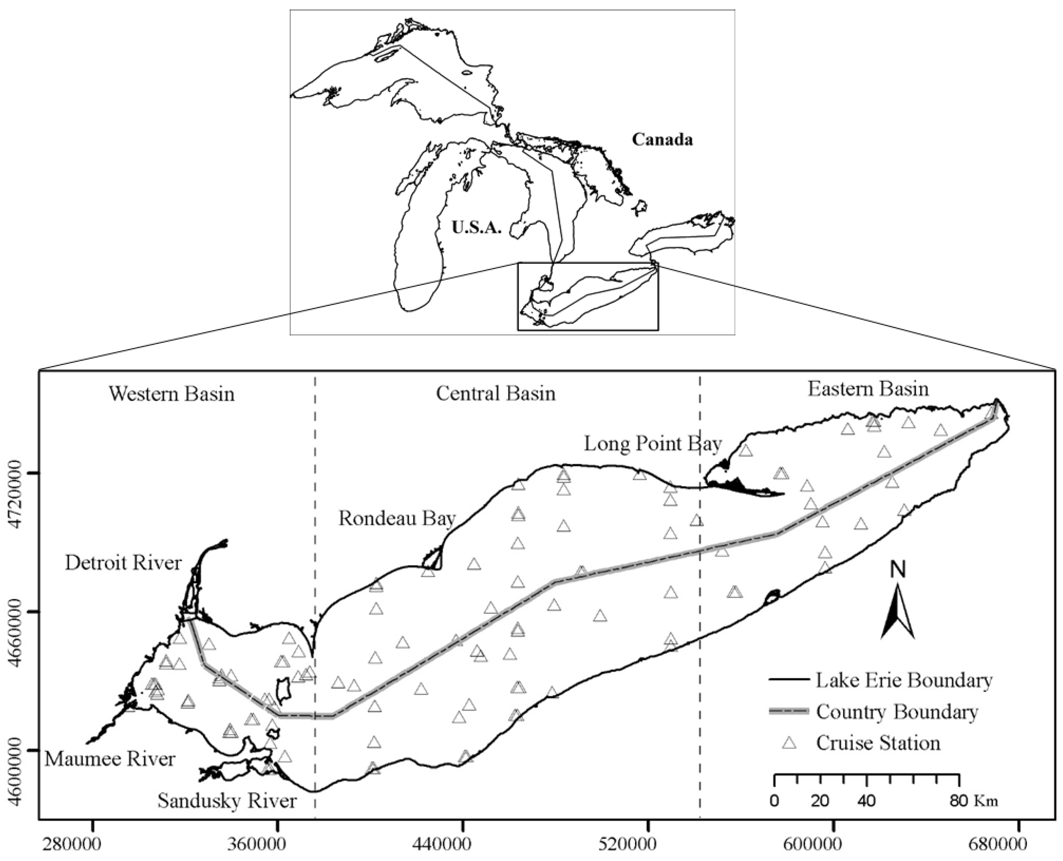
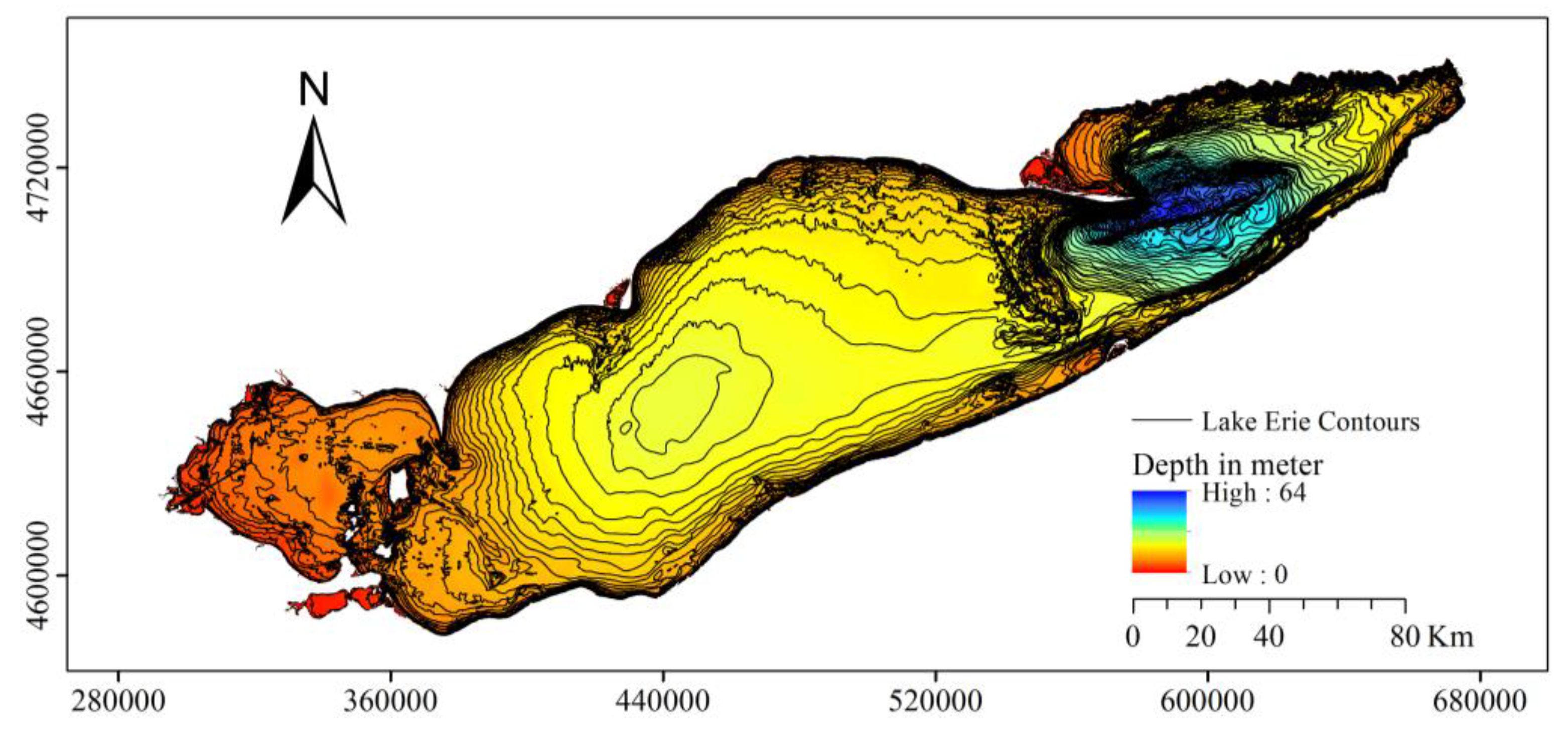
2.1. Study Site

Lake Erie (42°11′N, 81°15′W; Figure 1) is the smallest (by volume), the shallowest, and the warmest of the Laurentian Great Lakes [21]. It is a monomictic lake (with occasional dimictic years) covering an area of 25,700 km², with average and maximum depths of 19 m and 64 m, respectively [22]. The lake is naturally divided into three basins of different depths: the shallow western basin, the central basin, and the deep eastern basin (

Table 1. Lake Erie Basins Information (source: [23]).

Lake Erie	Mean Depth (m)	Maximum Depth (m)
West Basin	7.4	19
Central Basin	18.3	25
East Basin	25	64

). The basins are separated approximately based on the Lake Erie Islands (~82°49′W) and the Long Point-Erie Ridge (~80°25′W) (Figure 1) [1]. River discharge into Lake Erie originates mostly from the St. Clair River and Lake St. Clair through the Detroit River. Other smaller rivers and streams in the territory of Lake Erie also contribute to water inflow into the lake. Lake Erie drains into Lake Ontario through the Niagara River and shipping canals [2,23].

Lake Erie is exposed to greater stress than any other of the Great Lakes due to agricultural practices and urbanization in its surroundings. Chemically enriched runoff from agricultural lands in the basin flows into the lake. In addition, the lake receives the most effluents from wastewater treatment works [2,23]. Lake Erie has experienced substantial eutrophication over the past half century due to excess phosphorus loads from point and nonpoint sources producing algal blooms [21]. In general, phosphorus concentration in Lake Erie decreases from west to east and from near-shore to the offshore [24].

2.2. Field Measurements of Water Quality Parameters

Sample collection in Lake Erie was conducted on board of the Canadian Coast Guard ship Limnos during September 2004, May, July, and September 2005, May and June 2008, July and September 2011, and February 2012. A total of 89 distributed stations were visited to provide measurements of a wide range of optical properties as well as concentrations of the main CPAs in different locations of the lake (Figure 1).

Composite water samples were collected at all stations, during 2004 to 2012, from the surface mixed layer of the lake using Niskin bottles. The samples were filtered through a Whatman GF/F fiber filter (0.7 µm) in the field.

The filtered samples are then frozen and sent to the laboratory (the National Laboratory for Environmental Testing (NLET)) for extraction of the CPAs concentrations including chl-a. The chl-a measurement method is based on the trichromatic spectrophotometry following fixation using a 90% acetone solution and centrifugation. Absorption of the residue at specified wavelengths of 663 nm, 645 nm, and 630 nm are determined. Chl-a values are calculated using SCOR/UNESCO equations in the analytical range of 0.1–100 mg·m⁻³. The following trichromatic Equation 1 is recommended by SCOR/UNESCO to measure chl-a concentrations:

$$chl\_a=11.64 e_{663}-2.16 e_{645}+0.10 e_{630}$$

(1)

where chl-a is in µg·cm⁻³; and e₆₆₃, e₆₄₅, e₆₃₀ are the absorbances (cm⁻¹) of light path at 663, 645, 630 nm after subtracting the 750 nm reading [25]. The reported chl-a concentration also contains phaeopigments, which are degradation products of chl-a: phaeophytin and pheophorbide [26].

Secchi disk measurement is a worldwide accepted procedure to estimate water clarity in water bodies [27]. Light propagation and Secchi disk readings decreases exponentially due to light attenuation phenomenon [28]. SDD is regularly conducted during the Lake Erie cruises. Chl-a and SDD measurement methods follow the Ocean Optics Protocols for Satellite Ocean Color Sensor Validation [29,30].

2.3. Satellite Data and Processing

Launched by the European Space Agency (ESA) on 1 March 2002, the MERIS sensor was one of the instruments operating on the Envisat polar-orbiting satellite platform. Contact was lost with Envisat on 8 April 2012, which marked the end of the mission. MERIS was primarily dedicated to ocean color studies. MERIS was a push-broom imaging spectrometer that could measure the solar radiation reflected from the Earth’s surface in a high spectral and radiometric resolution (15 spectral bands across the range 390 nm to 1040 nm) with a dual spatial resolution (300 and 1200 m). MERIS scanned the Earth with global coverage every 2–3 days.

In this study, CC L2R (Version 2) MERIS reflectance full resolution images with full or partial coverage of Lake Erie between September 2004 and February 2012 were acquired through the Calvalus on-demand processing portal. The CC MERIS Level 2R product is generated using an atmospheric correction algorithm applied to the Level 1P product, which is a refined top of atmosphere radiance product with improved geolocation, calibration, equalization, smile correction, in addition to precise coastline and additional pixel characterization information (e.g., cloud, snow). The atmospheric correction procedure is based on two processors implemented in the Basic ERS & ENVISAT (A)ATSR MERIS (BEAM) software (Version 5.0): the Case II Regional (C2R) lake processor and also glint correction processor [17]. A detailed description of C2R can be found in Doerffer and Schiller (2007) [31].

The MERIS images were selected to be within a 2-day time window of in situ water quality measurements for the study period (2004–2012). This criterion was set to maximize the number of possible satellite and in situ measurements match-ups; at the same time reducing the effect of time heterogeneity of water quality parameters, assuming that these parameters would not change significantly in this time frame. Atmospherically corrected MERIS L2R reflectance values were extracted from pixels covering the geographic location of the stations. A valid pixel expression was defined that excluded all pixels with properties listed in

Table 2. Flags of excluded pixels.

Level 1	Level 1P	Level 2
Glint_risk	Land	AOT560_OOR (Aerosol optical thickness at 550 nm out of the training range)
Suspect	Cloud	TOA_OOR (Top of atmosphere reflectance in band 13 out of the training range)
Land_ocean	Cloud_ambigious	TOSA_OOR (Top of standard atmosphere reflectance in band 13 out of the training range)
Bright	Cloud_buffer	Solzen (Large solar zenith angle)
Coastline	Cloud_shadow
Invalid	Snow_ice
	MixedPixel

. Spatial averaging of pixels surrounding the station could be a technical solution to increase the number of resulting match-ups, when the considered pixel is excluded due to flags [32]. However, the horizontal spatial heterogeneity of parameters over the lakes prevents the averaging analysis.

2.4. Water Quality Parameters Algorithms

Semi-empirical algorithms are based on the regression between individual bands or band ratios, and the dependent variables, which are chl-a and SDD in this study. Different combinations can be considered based on the 15 MERIS spectral bands. Lakes with various optical and biological properties can produce different levels of correlation with these band combinations. This makes the use of semi-empirical algorithms a robust approach that can work on the lake of interest and within the time period that data samples were collected. The best band combinations were determined from the highest calculated Pearson correlation coefficients (R) against the logarithmic scale of in situ measurements of water quality parameters. It has long been known that the chl-a concentration distribution in the ocean is lognormal [33]. Also, the logarithmic function linearizes the relationship of in situ observations to band ratios and makes the distribution more symmetric (normal) (see Section 3.1). Considering the optical complexity of Lake Erie (see Section 3.1), red and NIR bands are required to derive chl-a concentration. Therefore, the selected band ratio for estimating chl-a was chosen among MERIS bands centered at B05:560 nm, B06:620 nm, B07:665 nm, B008:681.25 nm, B09:708.75 nm, B10:753.75 nm, B12:778.75 nm, and B13:865 nm. The band ratio for deriving SDD was selected among the visible bands: B01:412.5 nm, B02:442.5 nm, B03:490 nm, B04:510 nm, B05:560 nm, B06:620 nm, B07:665 nm, and B08:681.25 nm.

Sampling-wise, the same in situ measurements are repeated in time (month) over Lake Erie during the study period. Multiple measurements per variable in space or time will generally result in correlated errors and clustered data, which violate the assumptions of regression methods. Accordingly, random effect of time has to be added to the error term of the general regression models to account for measurements being made in clusters of time. The effect of time on the variation of water quality parameters can be considered to differ on a monthly basis. Therefore, in situ data collected repeatedly over the same month are considered to be correlated and this is the reason LME is used in this study, and month is selected as the random effect. Also, the measurements for different stations are inter-dependent. Different locations can affect each other’s measurements, depending on their distance. Therefore, there is spatial dependency in in situ observations. To consider both random and fixed effects in the regression, a LME model approach was selected to handle the repeated measurements and also the spatial autocorrelation of in situ observations.

Separate LME models were developed between the logarithmic scale of in situ chl-a and SDD with selected individual bands or band ratios of MERIS atmospherically corrected reflectance. The models were then used to predict chl-a and SDD over Lake Erie at different times. A LME model allows the prediction to be made at the outermost level (level = 0: predictions only based on fixed effects, as it would be in a standard regression model), and the innermost level (Level ≠ 0: predictions based on estimated random and fixed effects).

2.5. Accuracy Assessment

Cross validation was performed to assess the accuracy of derived chl-a and SDD estimates. Ten rounds were repeated by splitting the in situ measurements into training (70%) and testing (30%) datasets. The model performance indicators were reported as the average over the iterations. The mean bias error (MBE) and the root mean square error (RMSE) were used as the model performance indicators to describe chl-a and SDD retrieval accuracies. The MBE, and RMSE statistics are defined as follows:

$$RMSE=\sqrt{mean[{\left(x_{p{r}_i}-x_{ob{s}_i}\right)}^2]}$$

(2)

$$MBE=mean\left(x_{p{r}_i}-x_{ob{s}_i}\right)$$

(3)

where $x_{p{r}_i}$ is the predicted value, and $x_{ob{s}_i}$ is the observed value of the quantity which is measured in the field. Predicted and observed values should have the same scales. Therefore, the calculation of RMSE and MBE in logarithmic scale were performed on log-transformed in situ observations (algorithms’ output were already in the logarithmic scale). The RMSE is a comprehensive metric as it combines the mean and variance of the error distribution into a single term [34]. MBE also reveals the systematic errors [18].

Statistical analyses including: (1) finding the best band ratios using the MERIS atmospherically corrected reflectance, based on correlation with in situ observations; (2) development of LME models (regression method) based on selected band ratios and in situ observations; and (3) cross validation were performed in the R programming language (Version 3.2.1) [35].

3. Results

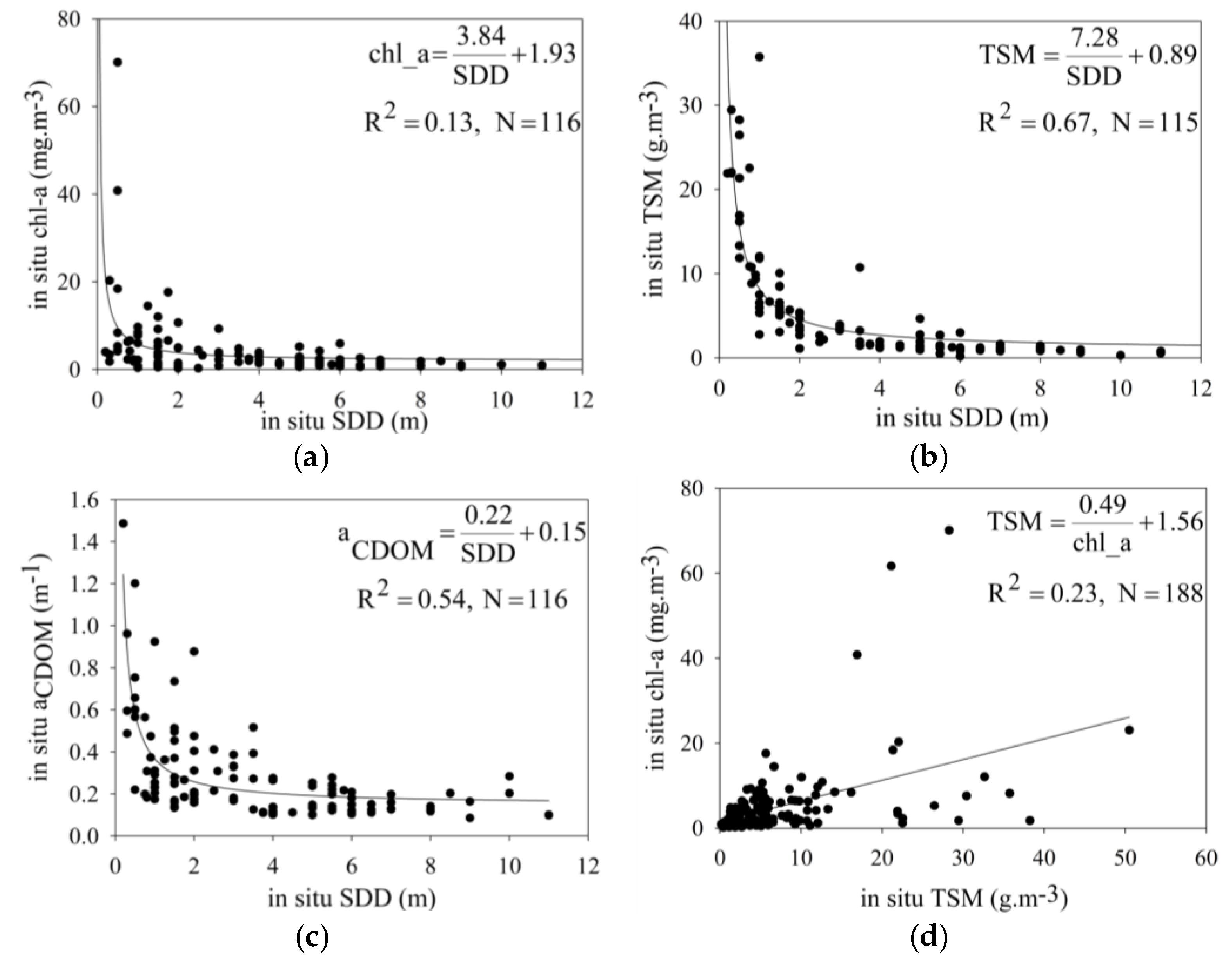
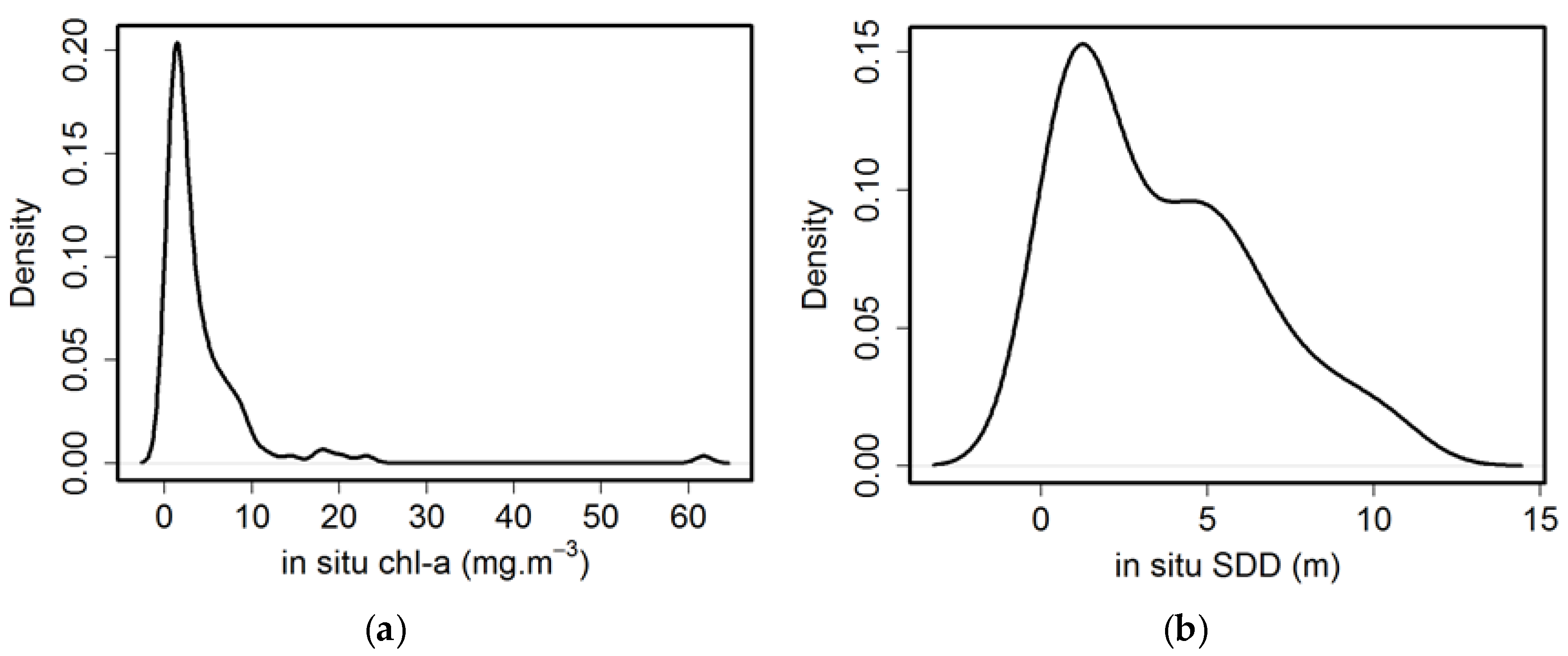
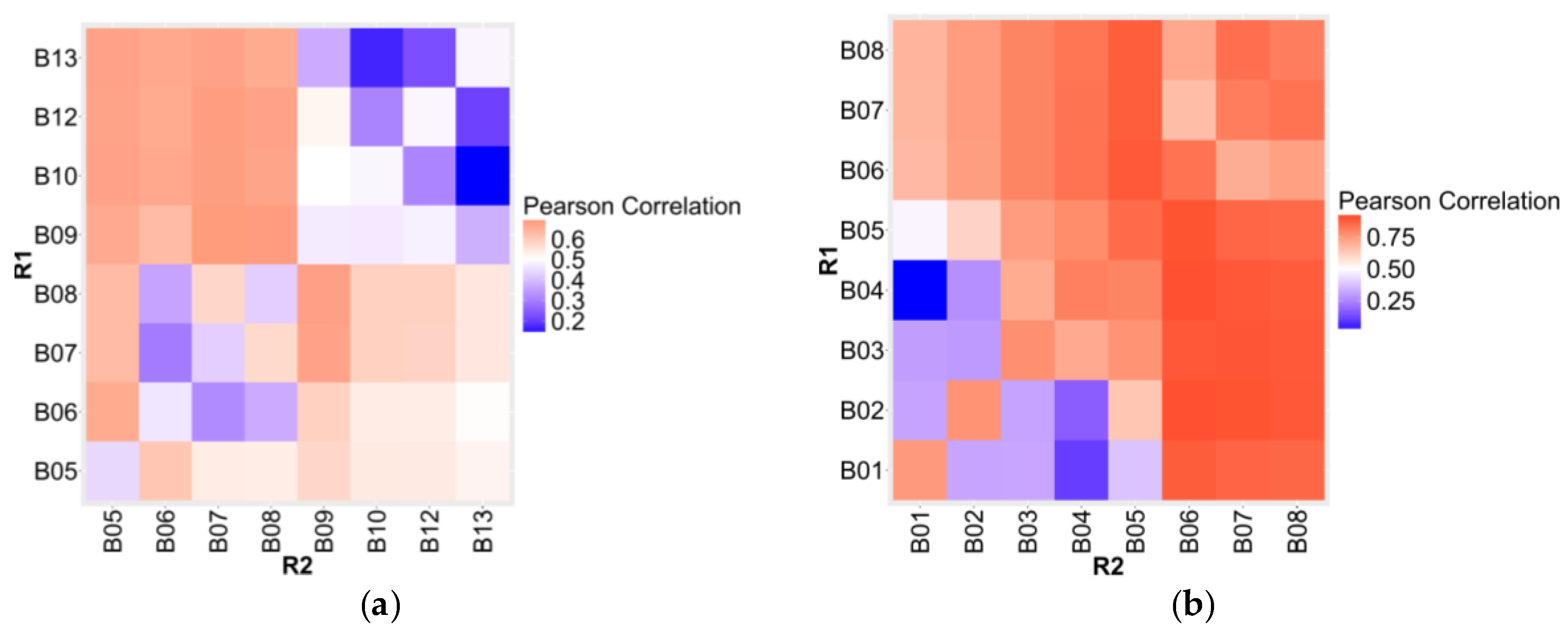
3.1. Lake Erie Optical Properties

Descriptive statistics of various bio-optical parameters measured in Lake Erie over the 2004–2012 period are summarized in

Table 3. Descriptive statistics of in situ measurements for Lake Erie (2004–2012). N is the number of times samples were collected at stations. St. dev. is standard deviation. Chl-a is in mg·m⁻³ and total suspended matters (TSM) is in g·m⁻³, a_CDOM in m⁻¹, and Secchi disk depth (SDD) in m.

	N	Min	Max	Mean	St. dev.
Chl-a	190	0.20	70.10	4.27	7.82
TSM	190	0.18	50.50	5.75	8.00
aCDOM	160	0.04	2.36	0.31	0.33
SDD	117	0.20	11.00	3.69	2.68

.

Figure 2 shows the contribution of different water constituents to water clarity in Lake Erie by investigating correlations between the concentrations of chl-a and TSM, and also absorption of CDOM in 440 nm (a_CDOM(440)) with the measured SDD. The graphs reveal that the concentrations of chl-a, TSM, and a_CDOM(440) are correlated with SDD over the period of measurements. TSM and to a lesser extent CDOM are important contributors to water clarity observed in Lake Erie with coefficient of determination (R²) values of 0.67 and 0.54, respectively. There is a low correlation between in situ measured chl-a and TSM demonstrating that these CPAs are non-covarying and independent.

The relative contribution of TSM compared to CDOM can be reduced in microtidal estuaries, or depending on the bathymetry of the lake [36]. In shallow Lake Erie, re-suspension of bottom sediments leads to higher water turbidity. Also, the Detroit and Maumee rivers contribute large sediment loads into the western basin of the lake. Kemp et al. (1997) identified the regions off Long Point and the mouths of these two rivers as the points of highest sedimentation rates in the lake [37]. The study of Binding et al. (2012) identified these zones as the highest turbid areas in the lake, confirming that TSM plays a major role in optically complex Lake Erie [1].

Based on the results presented in Table 3 and in Figure 2, Lake Erie can be classified as a typical Case II water system where other water constituents play a major and independent role in its low water clarity, besides chl-a concentration. Therefore, red and NIR reflectances are consistently the most reliable and expedient remote sensing variables in predictive algorithms for chl-a concentrations assessments in Lake Erie [11]. Figure 3 shows the probability density function (PDF) of in situ chl-a and SDD in Lake Erie. The PDFs for both variables demonstrate a lognormal distribution. Therefore, logarithmic transformations of chl-a concentration and SDD are used to develop the regressions.

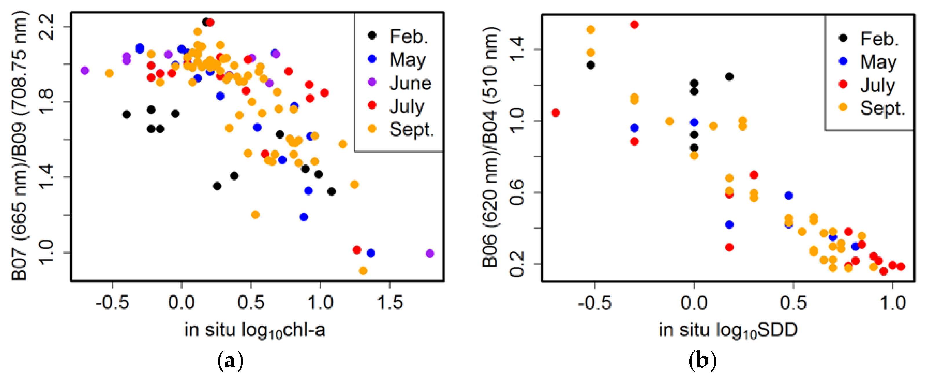
3.2. Linear Mixed Effect Models Calibration

The natural variation of the water quality parameter being measured determines the required period of concurrency between satellite overpasses and in situ observations [38]. In this study, satellite images were selected in a 2-day time window of in situ data collection. Using this criterion resulted in 16 MERIS CC L2R images being available for analysis. Applying defined flags produced 117 (60) pairs of atmospherically corrected reflectance and in situ chl-a (SDD) observations.

Pearson correlation (R) coefficients were calculated from MERIS bands or band ratios against the logarithmic scale of chl-a concentration and SDD measurements to select the best band or band ratios for the regression analysis of chl-a and SDD, separately. Figure 4 shows the range of correlation coefficients between the parameters of interest (chl-a and SDD) in logarithmic scale and both individual bands and band ratios of atmospherically corrected reflectance. The ratio of B07:665 nm to B09:708.75 nm has the highest correlation with chl-a concentration (R = −0.68) and the ratio of B13:865 nm to B10:753.75 nm the weakest correlation (R = −0.14). The highest and lowest correlation coefficients between SDD measurements and individual spectral bands or the ratio of them are observed for the band ratio of B06:620 nm to B04:510 nm (R = −0.90) and ratio of B04:510 nm to B02:442 nm (R = −0.16), respectively. From this analysis, band ratio B07:665 nm to B09:708.75 nm and band ratio of B06:620 nm to B04:510 nm were selected to investigate their predictive capability in estimating chl-a concentration and SDD, respectively, using LME regression models.

Resulting scatterplots of selected band ratios against in situ data are shown in Figure 5 for chl-a concentration and SDD measurements.

The LME models were developed from the relationships between selected band ratios and the logarithmic scale of chl-a and SDD. The month of in situ data collection represented the random effect due to repeated measurements in time. Random slopes and intercepts were considered for each group of measurements in a single month. Goodness of fit (r-squared; R²) for the outermost and innermost levels of prediction was 0.49 and 0.56 for chl-a and 0.78 and 0.83 for SDD, respectively. Therefore, the innermost level of predictions was used to predict chl-a concentration and SDD, with different values of slope and intercept for each month. The model developed for chl-a has average values of −1.16 (standard deviation: 3 × 10^–5, standard error: 0.1) and 2.44 (standard deviation: 0.12, standard error: 0.2) for slope and intercept, and the model developed to predict SDD has average values of −1.04 (standard deviation: 0.09, standard error: 0.08) and 0.99 (standard deviation: 0.05, standard error: 0.08) for slope and intercept. The estimated slope and intercept values for both models are significant (p < 0.005). The derived models are summarized using only the fixed effects as follows:

$${\log }_{10}\left(chl\_a\right)= \frac{B07\left(665\text{ nm}\right)}{B09 \left(708.75\text{ nm}\right)}\times \left(-1.16\right)+2.44$$

(4)

$${\log }_{10}\left(SDD\right)=\frac{B06 \left(620\text{ nm}\right)}{B04 \left(510\text{ nm}\right)}\times \left(-1.04\right)+0.99$$

(5)

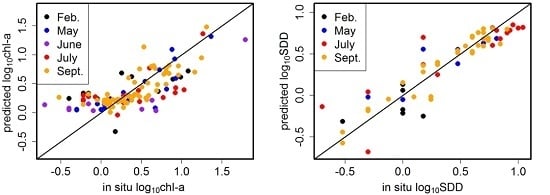
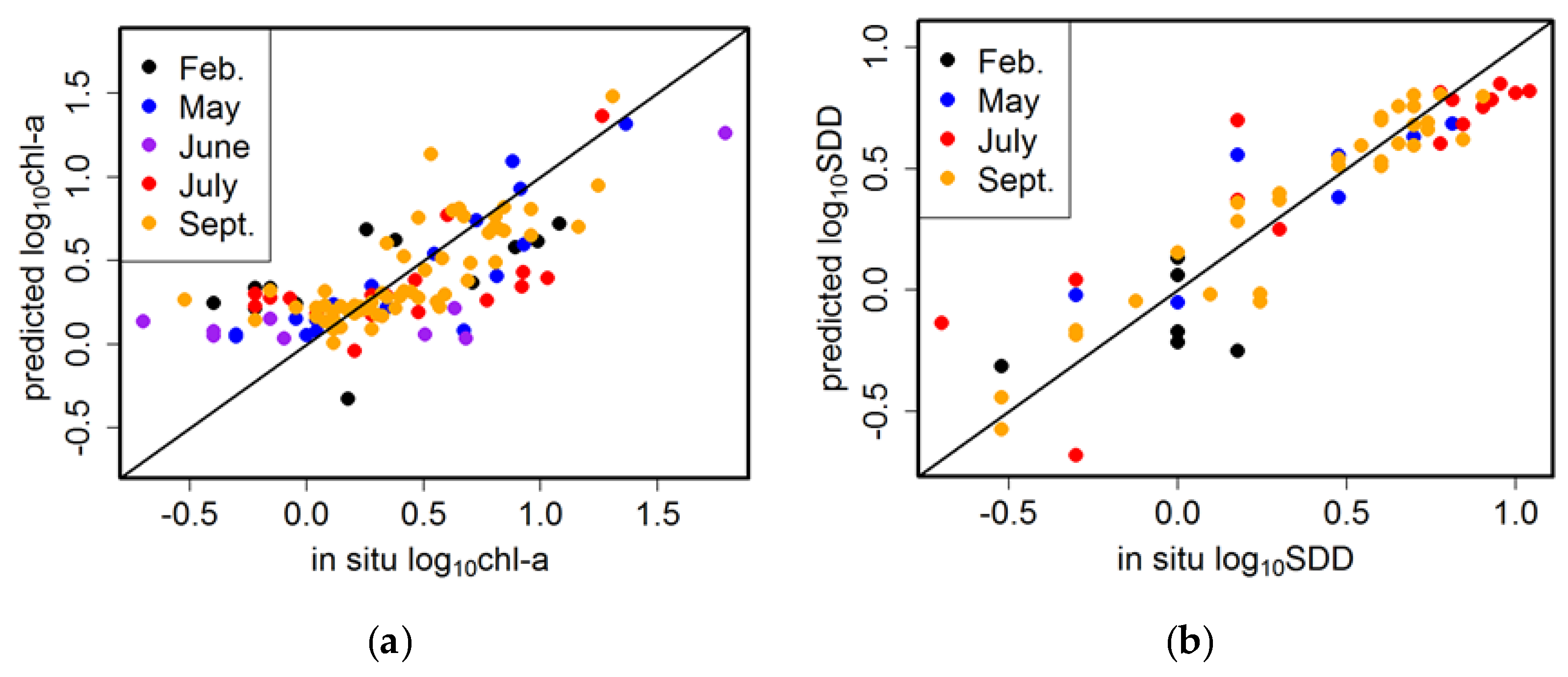
3.3. Evaluation of Linear Mixed Effect Models

The model performance indicators were derived for both models. Chl-a concentration is estimated with RMSE and MBE values of 0.31, and 0.018, respectively, in a logarithmic scale (N = 117; in the actual scale of chl-a: RMSE = 2.48 mg·m⁻³, MBE = −0.58 mg·m⁻³). SDD is predicted with RMSE value of 0.19 and MBE value equal to 0.006 in a logarithmic scale (N = 60; in the actual scale of SDD: RMSE = 1.40 m, MBE = −0.25 m). Comparisons between the measured and predicted log₁₀chl-a and log₁₀SDD using the LME models show that the values are in close agreement with paired observations, mostly evenly distributed along the 1:1 line (Figure 6). The chl-a model is, however, not sensitive enough to detect changes in low concentrations (below 0.1 in logarithmic scale, ca. 1 mg·m⁻³) and, as a result, the predicted values are not showing the variations corresponding to the small amount of in situ chl-a concentration measurements.

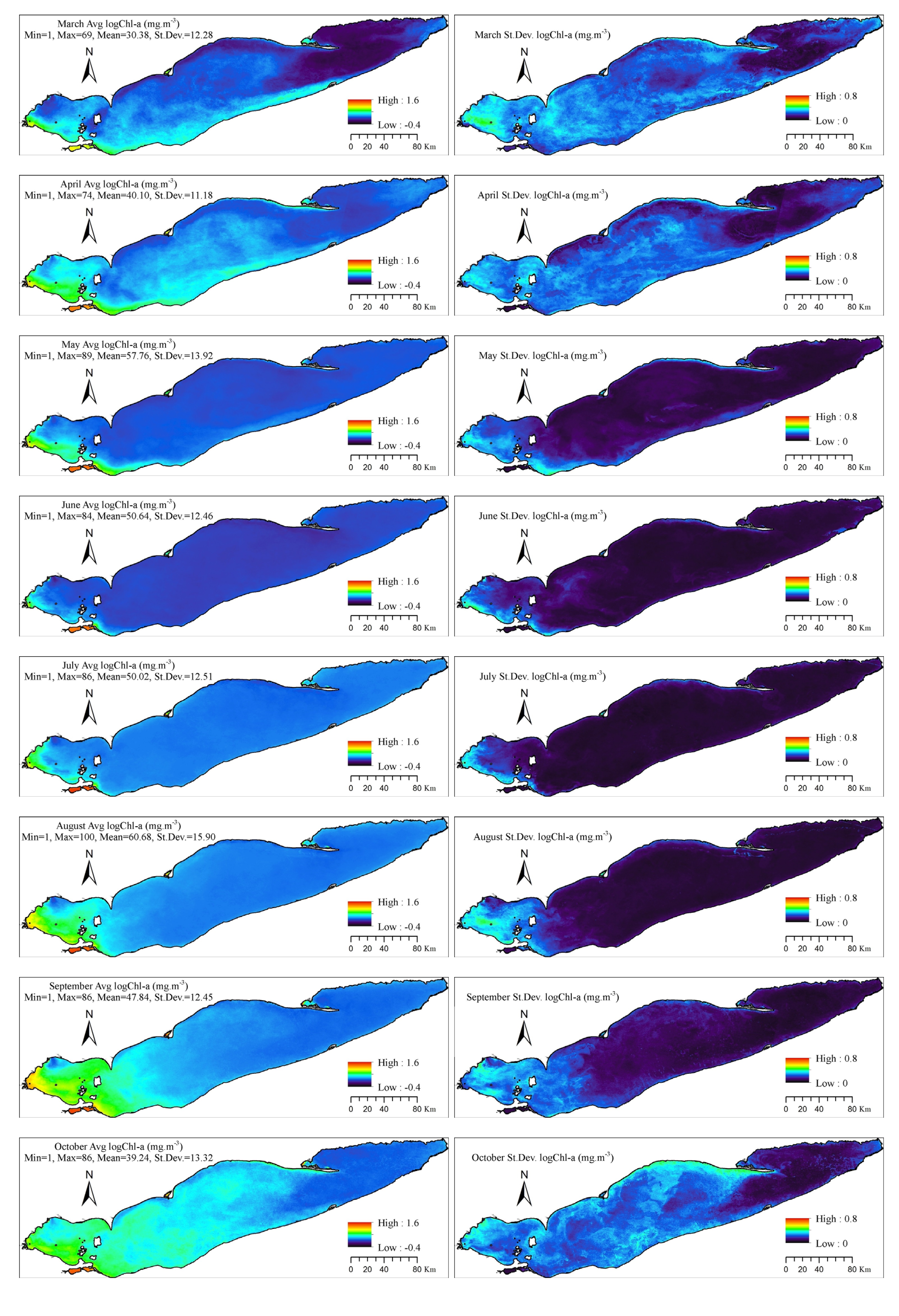
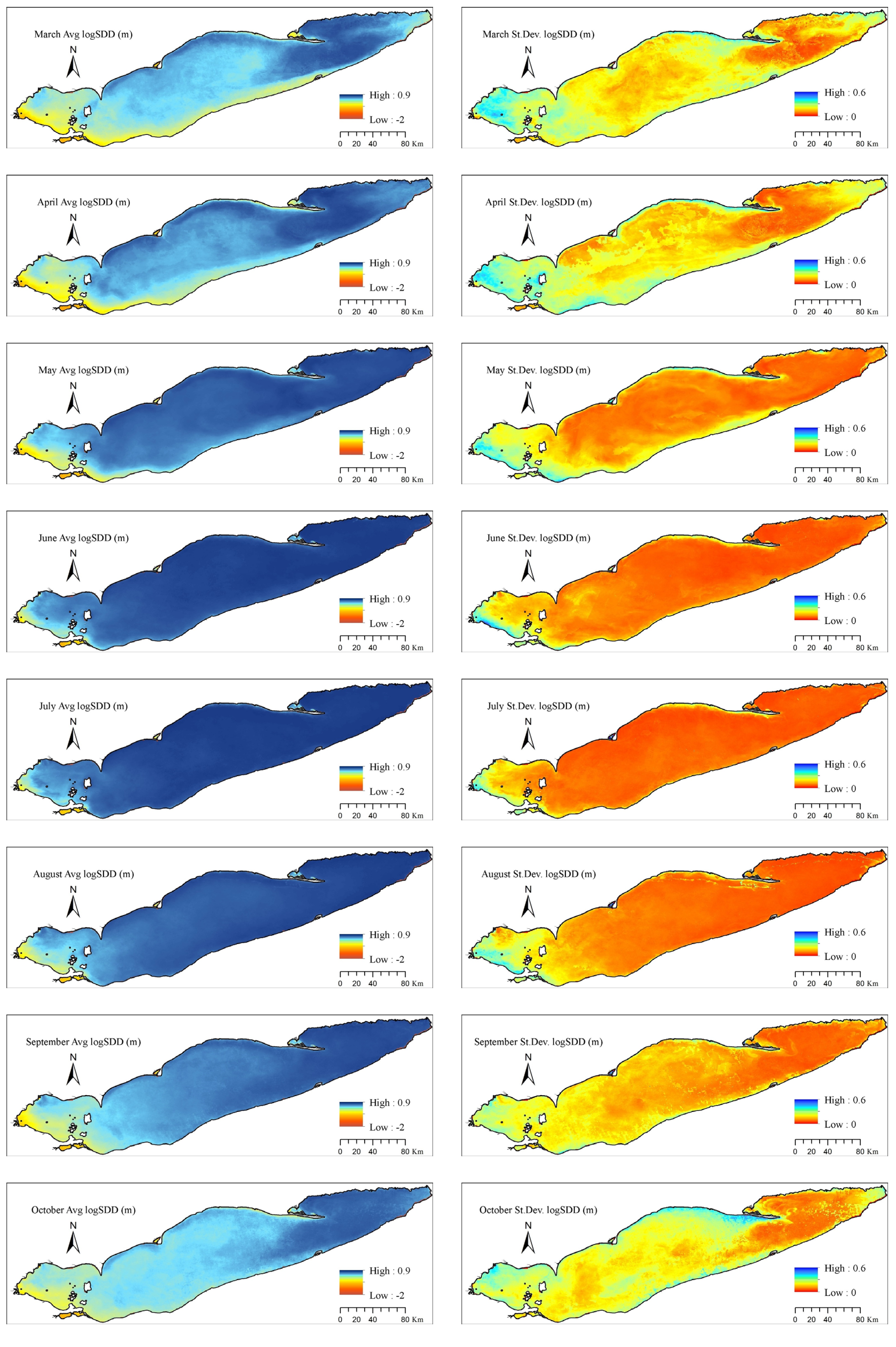
3.4. Spatial and Temporal Variations of Chl-a and SDD

The average chl-a concentration and SDD for each month between 2005 and 2011 are shown in Figure 7a and Figure 8a. In situ data in 2004 were only collected in September, and the values were not estimated for the months before September. Also, the Envisat satellite stopped operating in April 2012, hence there were no full year time series estimated for 2004 and 2012. These years were therefore disregarded in the time series analysis below. The statistics related to the number of available pixels for each month is included in Figure 7a, which are the same for SDD measurements.

The three basins of Lake Erie are characterized by distinct physical, chemical, biological, and optical properties. The highest chl-a concentrations and turbidity are experienced in different times of the year for each basin. The western basin always experiences a more intense algal bloom compared to the two other basins, with the most and least concentrations in September (6.62 ± 4.67 mg·m⁻³)–October (4.83 ± 3.67 mg·m⁻³) and June (2.39 ± 3.68 mg·m⁻³), respectively. Lake Erie’s central basin experiences spring bloom in April (2.08 ± 0.67 mg·m⁻³) and a more intense bloom in fall (October: 2.80 ± 0.79 mg·m⁻³). The eastern basin shows the least chl-a concentrations of the three basins, and its highest algal intensity occurs in summer (August, 1.78 ± 1.27 mg·m⁻³). Some more specific areas of the lake are affected by prolonged intense algal bloom, including Maumee Bay, Sandusky Bay, Rondeau Bay and Long Point Bay. The highest SDD values for the full lake are estimated in July (5.38 ± 1.16 m), whereas the lowest SDD estimates are observed in March (2.44 ± 1.20 m) and October (2.52 ± 1.13 m). There is also a north-south gradient noticeable in both chl-a concentration and SDD in western Lake Erie.

Standard deviations of chl-a (Figure 7b) and SDD (Figure 8b) were also calculated for each month (March to October) to show variations of log₁₀chl-a and log₁₀SDD from the average values. Figure 7 and Figure 8 show that the greatest variability occurs in the western basin for both log₁₀Chl-a and log₁₀SDD, with its largest variability in March. The least variations in chl-a concentration and SDD patterns occur in the offshore areas and eastern basin.

4. Discussion

4.1. Linear Mixed Effect Model Results

Our study agrees with previous studies to the effect that Lake Erie is to be considered as a Case II water. O’Donnell et al. (2010) employed modern instrumentation to measure IOPs and AOPs in the western basin of Lake Erie. The study also concluded that the characterization of IOPs and AOPs supports the fact that the western basin of Lake Erie is an optically complex Case II system. Therefore, in such case, red and NIR band ratios are the most reliable predictors in regression algorithms to estimate chl-a concentration in Lake Erie. Results from the LME models calibration show that the band ratio of B07:665 nm to B09:708.75 nm is highly negatively correlated with the variations of chl-a concentration in Lake Erie. Gitelson et al. (2007) applied a two-band model, as the special case of a conceptual three-band model [39], to the turbid (Case II) waters of Chesapeake Bay to estimate chl-a concentration [40]. The tuning process found the ratio of 720 nm to 670 nm as the optimal spectral band ratio, with the maximal R² of 0.79 in a positive correlation. Water samples collected from Chesapeake Bay contained widely variable chl-a concentrations (9 to 77.4 mg·m⁻³), when SDD ranged from 0.28 to 1.5 m. Duan et al. (2010) also found the band ratio of 710/670 nm to be positively correlated with chl-a concentration in eutrophic Lake Chagan with R² = 0.70. Chl-a concentration in this lake was between 6.40 and 58.21 mg·m⁻³ and SDD rarely exceeded 0.50 m [11]. Simis et al. (2005, 2007) correlated the absorption of chl-a to MERIS band ratio of 708.75 to 665 nm for turbid, cyanobacteria-dominated lakes in the Netherlands and Spain. Hicks et al. (2013) reported that the logarithmic scale of SDD measurements and logarithmic scale of Landsat 7 ETM+ band ratio of B01(0.450–0.515 nm)/B03(0.630–0.690 nm) were positively correlated with a high correlation (R = 0.82). This study was conducted for shallow lakes (ranging from 1.8 to 8.7 m depth) in the Waikato region in New Zealand, with SDD in situ observations varying between 0.005 and 3.78 m [41]. In our study, the highest correlation between MERIS band ratios and SDD variations in Lake Erie was estimated for the band ratio of B06:620 nm to B04:510 nm.

The selected band ratios were used to develop two separate LME models to estimate chl-a concentration and SDD in Lake Erie. The models were evaluated using the testing data in a cross validation approach. Results showed that LME model was in a high agreement with the chl-a in situ observations with RMSE and MBE values of 0.31, and 0.018, respectively, in a logarithmic scale. The overestimation of chl-a concentration derived from the LME model can be attributed to the contribution of TSM in the red/NIR region of the spectrum that is not necessarily correlated with chl-a concentration. In turbid waters such as Lake Erie, the signals measured in the red and NIR regions can no longer be attributed to the chl-a concentration absorption and fluorescence and water alone, while TSM can also confound the signal [1]. Although, formation of blooms in a thick surface layer can dominate the reflectance and eliminate much of the contribution of TSM to reflectance [42]. The LME model is particularly overestimating while not showing sensitivity to chl-a values lower than 0.1 in logarithmic scale (see Figure 6a). Binding et al. (2013) assessed the sensitivity of maximum chlorophyll index (MCI; measures a peak in red/NIR region near 708 nm relative to a baseline which is drawn between two suitable wavelengths) to mineral sediments. The modeling results in this study suggested that the sensitivity of MCI to mineral turbidity particularly increases at low chlorophyll concentrations when mineral sediments can contribute to reflectance and lead to substantial increase in the resulted MCI [42]. This study derived a strong linear relationship between in situ MCI and chl-a concentration in Lake Erie with R² value of 0.70, suggesting a minimal contamination of the MCI signal from sediments under intense surface algal blooms [42]. A blue/green band ratio algorithm was tested for western basin Lake Erie in Ali et al. (2014) and resulted in R² value of 0.46. For chl-a concentrations below 6 mg·m⁻³, a closer 1:1 relationship with the in situ measurements was derived [43]. However, Witter et al. (2009) found systematic overestimation of low chl-a concentration in the western basin of Lake Erie applying regionally calibrated quadratic algorithms (employing blue/green bands as the predictor) on SeaWiFS imagery. Therefore, the difficulties associated with estimation of chl-a using blue/green band ratio algorithms in turbid, optically complex waters is demonstrated. In this region of spectrum, CDOM confounds the signals as well as TSM and chl-a concentrations [44].

Moore et al. (2014) applied a blending approach, to manage the selection between two band ratio algorithms in the blue/green and red/NIR regions, based on the optical water type classification of Lake Erie. RMSE and MBE values were 0.32, and 0.023 in logarithmic chl-a units [18]. Sá et al. (2015) evaluated CC chl-a products including: OC4, NN, and merged products, for the Western Iberian coast. The uncertainty estimation analysis was presented on the logarithmic scale of chl-a (0.249 < RMSE < 0.278, 0.139 < MBE < 0.200; for 3-hour time intervals) [45]. The derived LME model for SDD estimation resulted in RMSE and MBE values of 0.19, and 0.006, in logarithmic units. Wu et al. (2008) estimated SDD in Poyang Lake in China from two multiple regression models. The models were developed using spectral bands of Landsat TM and MODIS, separately. In both models the blue and red bands were used in the regression. The logarithmic scale of SDD was predicted with RMSE values of 0.20 and 0.37 for the models, respectively [14]. Results from our study indicate that the LME models can be used to derive the bio-optical quantities; the models provide accuracies comparable to that of other studies. A good agreement between the selected band ratios (B07/B09 for chl-a and B06/B04 for SDD) of atmospherically corrected CC L2R MERIS data and in situ measurements of chl-a and SDD in logarithmic scale were derived for Lake Erie for the 2004–2012 study period.

4.2. Interpretation of Spatial and Temporal Variations in Chl-a and SDD

Monthly maps of chl-a concentration and SDD for Lake Erie (Figure 7 and Figure 8) show that Maumee Bay, Sandusky Bay, Rondeau Bay and Long Point Bay have persistent intense algal blooms. These specific areas are known to experience cyanobacteria blooms due to constant nutrient enrichment [1]. Maumee River drains a large watershed which is dominated by agricultural fields, and also is a tributary of the largest storm runoff within the Lake Erie basin [46,47]. There was also a north-south gradient in western basin for chl-a concentration and SDD estimations. This gradient can be explained by inflows from the Detroit River. The Detroit River is a major source of flows from the upper Great Lakes into Lake Erie, which carries contaminated sediments and nutrients from a highly urbanized and industrialized watershed into western Lake Erie [1,48]. However, the comparatively clearer water that is carried through this river from the upper Great Lakes can create the north-south gradient in Lake Erie [1]. Also, Dolan (1993) reported that municipal phosphorus loads from US sources have a higher magnitude compared to the Canadian ones during the period 1986–1990 [49]. Therefore, if the same trend of phosphorus loads in those years occurs during the time period of this study, the observed differences between north and south near-shore algal productivity can be enlightened [1].

Re-suspension, shoreline erosion and loading from different sources such as rivers are among the most important factors influencing SDD estimates. Wind, as the primary source of kinetic energy, affects the sediment redistribution in the water column in Lake Erie [50]. The high-energy and short-lived winter storms are a characteristic of Lake Erie wave climate that interrupts a long period of relative calm weather [47]. These strong storms usually occur before the lake freezes (in October, November, and December) and also in spring after ice break-up (March and April) [1]. However, it should be noted that the depth of the lake directly affects the amount of kinetic energy generated by wind. In other words, the re-suspension of sediment loads generated by wind in the shallower areas can be more pronounced than in the deeper areas of Erie. Comparing SDD estimates (Figure 8) with lake depths in Figure 9, it can clearly be seen that the deeper areas are relatively clearer, while the shallow areas are more turbid. The maximum depth of the western basin is only 11 m [51]. Hence, being the shallowest area, the western basin is the most vulnerable to physical processes such as re-suspension. Therefore, re-suspension of TSM can result in a prolonged constant turbidity in West Erie basin. Rivers and streams can supply suspended matters to the lake; and result in SDD reduction. The Detroit River (1.6 million tons/year) and the Maumee River (1.2–1.3 tons/year) have the major role in loading fine-grained sediments into Lake Erie [52]. Rainstorms can even strengthen the contribution of river discharges to load sediments in the lakes [53].

The largest variations in chl-a concentration (Figure 7) and SDD (Figure 8) occur in the western basin in March. This area of the lake is the estuary of the Detroit River and close to Maumee Bay and Sandusky Bay. Precipitation and runoff during this time of year, after the ice break-up period on the lake, cause more variations in nutrient availability and water column re-suspension effect on algal biomass and lake turbidity. The offshore areas and eastern basin have the least variations in chl-a concentration and SDD patterns. These lake sections appear to experience low fluctuations in the availability of required resources for algal bloom such as nutrients. Also, eastern basin of Lake Erie is the deepest with an average depth of 24 m (max depth = 64 m). Physical processes such as re-suspension have the least effect on the turbidity and its variations in the deep parts of the lake, as opposed to the shallow western basin.

Meteorological forcings can also have an impact on the magnitude and timing of blooms. In general, a temperature increase leads to higher rates of photosynthesis and therefore to a greater phytoplankton growth rate under adequate resource supplies such as nutrients and light. Light-limited photosynthesis rate is insensitive to temperature, whereas a light-saturated one increases with temperature [54]. The resource availability of light and nutrients can be accompanied by vertical mixing. Therefore, the seasonal cycles of stratification and wind-induced vertical mixing are the key variables that condition the growth rate of phytoplankton in the water column [54]. Stratification results in a nutrient-depleted condition at the water surface, when the upward flux of nutrients from the deep water layers is suppressed. Also, the overall impact of windiness decreases light availability in the lower depth due to re-suspension of sediments [54]. As a result, the balance found between meteorological forcings, which sometimes can have opposite effects, is one of the driving factors determining the bloom condition. Phytoplankton production is a complex function and can be controlled by resources dynamics, species composition, and predator–prey interactions in the ecosystem [54].

4.3. Limitations and Uncertainties of the Applied Linear Mixed Effect Model on MERIS

The influence of other existing particulates in a Case II water, such as CDOM and TSM, will be significantly decreased employing the chosen wavelengths to develop the chl-a LME model, as opposed to empirical blue-to-green band ratio algorithms. The absorption of CDOM is greatest in the blue region and certainly decreases exponentially with increasing wavelength, being near negligible in the NIR for the majority of the Great Lakes waters [1]. The wavelengths (665 and 708.75 nm) have a minimal sensitivity to other CPAs, but the absorption and scattering of suspended matters can still interfere within the chl-a algorithm selected wavebands. Increasing sediment loads result in the reflectance peak to move from blue to green to red in turbid waters [55]. Therefore, the semi-empirical models need to be tuned for each water body of interest characterized by different optical properties, in order to obtain the optimized wavelengths that can discriminate algal from suspended matters, and result in improved retrieval accuracy. Binding et al. (2012) presented a method to discriminate algal from particulate matters. The method simultaneously extract algal and suspended matters for Lake Erie from red and NIR bands of MODIS-Aqua sensor. The study resulted in estimated concentrations in close agreement with in situ observations with RMSE and R² values of 2.21 mg·m⁻³ and 0.95 for chl-a and 1.04 g·m⁻³ and 0.91 for TSM, respectively [1].

In addition, one has to consider that there is a relatively higher level of errors in computing remote sensing reflectance at longer wavelengths. Water absorption in red-NIR is strong and produces less remote sensing reflectance and, accordingly, a lower signal-to-noise ratio. This error is even higher in the case of clear waters where there is a low concentration of CDOM and TSM to produce remote sensing reflectance [1]. In Lake Erie, however, the contribution of suspended and dissolved matters in remote sensing reflectance is high enough to allow the use of the proposed wavelengths from this study and produce a strong agreement between the modeled and observed values.

Atmospheric corrections are a critical step over water bodies, since the radiance signal emerging from the water column is much less than that of land. Atmospheric corrections become even more challenging in highly turbid inland and coastal waters where the ‘black pixel’ assumption of negligible water-leaving radiance in the near-infrared (NIR) is no longer valid due to scattering from suspended matters [50]. Thus, typical atmospheric corrections fail and other schemes based on radiative transfer models or other approaches are required [13]. The accuracy of atmospheric correction algorithms used in different models is very important to evaluate the satellite-derived water quality products. However, in a band ratio algorithm with bands near each other, atmospheric effects are normalized [13].

In the northern part of the western basin of Lake Erie, benthic algae can be seen at the surface when the water is clear enough. Consequently, in some remote sensing methods, benthic algae can contribute to the remote sensing reflectance [1]. In the present study, however, there is no need to distinguish benthic algae from surface algae. The rapid in-water attenuation of the wavelengths selected in this study for chl-a model means that the remote sensing reflectance in these wavelengths originates mostly from the upper 30 cm of water column in the lake (depends on the diffuse attenuation coefficient) [50]. Therefore, there is no contribution of reflectance from algae at the bottom of the lake or subsurface. The estimated chl-a concentration is attributed to the surface or near surface algae even in the shallow areas or sections of the lake with clear water. The in situ samples to measure chl-a concentration in Lake Erie were collected from the surface mixed layer. There is a constant relationship between chl-a concentration at the surface and the one averaged over the mixed layer, as Lake Erie is shallow and exposed to strong wind-driven mixing to create a mainly mixed water column condition [50].

In situ data are required for algorithm evaluation purposes and also for parameterizing the LME models. The water quality parameters measured in the field can change at a scale smaller than that of the satellite image pixel resolution (300 m for MERIS), especially in Lake Erie due to different river inputs and wind effect. Thus, multiple measurements around stations are necessary to consider spatial heterogeneity. Also, the time lapse between satellite overpasses and in situ data collection may characterize a large change in the water quality parameter magnitude. The extent of these variations depends on the particular condition in the water body and defines the time window to be considered between satellite and in situ measurements. A time window of 3 h between satellite overpass and in situ data collection is recommended for open ocean waters [56]. However 2-day time window was selected for inland waters of Lake Erie to increase the number of matchups for validation and training purposes. There are also some uncertainties associated with in situ data collections. Over- or underestimation of chl-a concentration measurements in the field is inevitable when the collected samples contain all of the pigments, due to spectral absorption overlaps [57,58,59,60]. SDD measurements are subjective and may vary depending on the operator’s ability. In shallow water bodies, disk contrast disappears at a shorter depth due to bottom reflections. Also, the disk can reach the bottom of the shallow parts of the lake without disappearing [28], which is not the case in Lake Erie as the depth measured in the survey was always larger than SDD [1].

Although MERIS is no longer active, the upcoming Sentinel-3a and b satellite missions of ESA, which will each carry the OLCI (Ocean and Land Colour Instrument) sensor (heritage of MERIS), will mark a new era in the measurement of lake water quality parameters from space. OLCI has an optimized design to minimize sun-glint and will provide 21 spectral bands compared to the 15 bands available from MERIS. Therefore the band ratio selection is between a larger numbers of bands that are improved with regards to radiometric correction.

5. Conclusions

This paper presented and assessed a remote sensing approach that utilizes spectral bands in the red and NIR portions of the spectrum to estimate chl-a concentration, and visible bands to determine SDD from MERIS images obtained over Lake Erie for the 2004–2012 period. LME models were developed based on the selected bands and in situ measurements. This method presents advantages over the traditional regression models that are only based on fixed effects, and that do not consider the correlation that stems from repeated measurements in space and time. Also, the LME models for chl-a and SDD are semi-empirical models that, unlike the semi-analytical models, do not require detailed knowledge of the IOPs of the CPAs in water.

Despite the limitations of remote sensing methods, they can still be considered as providing a complementary approach for the estimation of parameters related to water optical properties for many lakes over large areas and with frequent temporal coverage. Measurements at an acceptable frequency are required in order to discern potential water quality problems associated with the lake. In situ measurements of water quality parameters at sufficient temporal and spatial resolutions are, on the other hand, problematic due to field logistics and extended periods without sampling as a result of changes in funding priorities by agencies. Remote sensing has the potential to infer the lake bio-optical/water quality parameters overcoming these concerns.

References

1. Binding, C.E.; Greenberg, T.A.; Bukata, R.P. An analysis of MODIS-derived algal and mineral turbidity in Lake Erie. J. Gt. Lakes Res. 2012, 38, 107–116. [Google Scholar] [CrossRef]
2. Daher, S. Lake Erie LAMP Status Report; Environment Canada: Burlington, ON, Canada, 1999. [Google Scholar]
3. Morel, A.; Prieur, L. Analysis of variations in ocean color. Limnol. Oceanogr. 1977, 22, 709–722. [Google Scholar] [CrossRef]
4. Zhao, D.; Cai, Y.; Jiang, H.; Xu, D.; Zhang, W.; An, S. Estimation of water clarity in Taihu Lake and surrounding rivers using Landsat imagery. Adv. Water Resour. 2011, 34, 165–173. [Google Scholar] [CrossRef]
5. McCullough, I.M.; Loftin, C.S.; Sader, S.A. Combining lake and watershed characteristics with Landsat TM data for remote estimation of regional lake clarity. Remote Sens. Environ. 2012, 123, 109–115. [Google Scholar] [CrossRef]
6. Tebbs, E.J.; Remedios, J.J.; Harper, D.M. Remote sensing of chlorophyll-a as a measure of cyanobacterial biomass in Lake Bogoria, a hypertrophic, saline–alkaline, flamingo lake, using Landsat ETM+. Remote Sens. Environ. 2013, 135, 92–106. [Google Scholar] [CrossRef]
7. Binding, C.E.; Greenberg, T.A.; Bukata, R.P. Time series analysis of algal blooms in Lake of the Woods using the MERIS maximum chlorophyll index. J. Plankton Res. 2011, 33, 1847–1852. [Google Scholar] [CrossRef]
8. McCullough, I.M.; Loftin, C.S.; Sader, S.A. High-frequency remote monitoring of large lakes with MODIS 500 m imagery. Remote Sens. Environ. 2012, 124, 234–241. [Google Scholar] [CrossRef]
9. Saulquin, B.; Hamdi, A.; Gohin, F.; Populus, J.; Mangin, A.; D’Andon, O.F. Estimation of the diffuse attenuation coefficient kdPAR using MERIS and application to seabed habitat mapping. Remote Sens. Environ. 2013, 128, 224–233. [Google Scholar] [CrossRef]
10. Odermatt, D.; Pomati, F.; Pitarch, J.; Carpenter, J.; Kawka, M.; Schaepman, M.; Wüest, A. MERIS observations of phytoplankton blooms in a stratified eutrophic lake. Remote Sens. Environ. 2012, 126, 232–239. [Google Scholar] [CrossRef]
11. Duan, H.; Ma, R.; Xu, J.; Zhang, Y.; Zhang, B. Comparison of different semi-empirical algorithms to estimate chlorophyll-a concentration in inland lake water. Environ. Monit. Assess. 2010, 170, 231–244. [Google Scholar] [CrossRef] [PubMed]
12. Bresciani, M.; Giardino, C. Retrospective analysis of spatial and temporal variability of chlorophyll-a in the Curonian Lagoon. J. Coast. Conserv. 2012, 16, 511–519. [Google Scholar] [CrossRef]
13. Matthews, M.W.; Bernard, S.; Winter, K. Remote sensing of cyanobacteria-dominant algal blooms and water quality parameters in Zeekoevlei, a small hypertrophic lake, using MERIS. Remote Sens. Environ. 2010, 114, 2070–2087. [Google Scholar] [CrossRef]
14. Wu, G.; Leeuw, J.D.; Skidmore, A.K.; Prins, H.H.T.; Liu, Y. Comparison of MODIS and Landsat TM5 images for mapping tempo–spatial dynamics of secchi disk depths in Poyang Lake national nature reserve, China. Int. J. Remote Sens. 2008, 29, 2183–2198. [Google Scholar] [CrossRef]
15. Kratzer, S.; Brockmann, C.; Moore, G. Using MERIS full resolution data to monitor coastal waters—A case study from Himmerfjärden, a fjord-like bay in the Northwestern Baltic Sea. Remote Sens. Environ. 2008, 112, 2284–2300. [Google Scholar] [CrossRef]
16. Pinheiro, J.; Bates, D.; DebRoy, S.; Sarkar, D. Linear and Nonlinear Mixed Effects Models. Available online ftp://ftp.uni-bayreuth.de/pub/math/statlib/R/CRAN/doc/packages/nlme.pdf (accessed on 16 May 2016).
17. Ruescas, A.; Brockmann, C.; Stelzer, K.; Tilstone, G.H.; Beltrán-Abaunza, J.M. DUE CoastColour Final Report, Version 1; Brockmann Consult: Geesthacht, Germany, 2014. [Google Scholar]
18. Moore, T.S.; Dowell, M.D.; Bradt, S.; Ruiz-Verdu, A. An optical water type framework for selecting and blending retrievals from bio-optical algorithms in lakes and coastal waters. Remote Sens. Environ. 2014, 143, 97–111. [Google Scholar] [CrossRef] [PubMed]
19. Kratzer, S.; Håkansson, B.; Sahlin, C. Assessing secchi and photic zone depth in the Baltic Sea from satellite data. AMBIO 2003, 32, 577–585. [Google Scholar] [CrossRef] [PubMed]
20. Fleming-Lehtinen, V.; Laamanen, M. Long-term changes in secchi depth and the role of phytoplankton in explaining light attenuation in the Baltic Sea. Estuar. Coast. Shelf Sci. 2012, 102–103, 1–10. [Google Scholar] [CrossRef]
21. Michalak, A.M.; Anderson, E.J.; Beletsky, D.; Boland, S.; Bosch, N.S.; Bridgeman, T.B.; Chaffin, J.D.; Cho, K.; Confesor, R.; Daloglu, I.; et al. Record-setting algal bloom in Lake Erie caused by agricultural and meteorological trends consistent with expected future conditions. Proc. Natl. Acad. Sci. USA 2013, 110, 6448–6452. [Google Scholar] [CrossRef] [PubMed]
22. Bootsma, H.A.; Hecky, R.E. A comparative introduction to the biology and limnology of the African Great Lakes. J. Gt. Lakes Res. 2003, 29, 3–18. [Google Scholar] [CrossRef]
23. Lake Erie LaMP Work Group. Lake Erie Lakewide Action and Management Plans (LAMPs); US Environmental Protection Agency: Chicago, IL, USA, 2000.
24. International Joint Commission Canada and United States. Lake Erie Ecosystems Priority, Scientific Findings and Policy: Recommendations to Reduce Nutrient Loadings and Harmful Algal Blooms; International Joint Commission: Washington, DC, USA, 2013. [Google Scholar]
25. UNESCO. Determination of Photosynthetic Pigments in Sea-Water; UNESCO Monographs on Oceanographic Methodology: Paris, France, 1966. [Google Scholar]
26. Environment Canada. Manual of Analytical Methods; Environmental Conservation Service—ECD; Canadian Communications Group: Toronto, ON, Canada, 1997. [Google Scholar]
27. Effler, S. Secchi disk transparency and turbidity. J. Environ. Eng. 1988, 114, 1436–1447. [Google Scholar] [CrossRef]
28. Civera, J.I.; Miró, N.L.; Breijo, E.G.; Peris, R.M. Secchi depth and water quality control: Measurement of sunlight extinction. In Mediterranean Sea: Ecosystems, Economic Importance and Environmental Threats; Hughes, T.B., Ed.; Nova Science: New York, NY, USA, 2013; pp. 91–114. [Google Scholar]
29. Mueller, J.L.; Bidigare, R.R.; Trees, C.; Balch, W.M.; Dore, J.; Drapeau, D.T.; Karl, D.; Heukelem, L.V.; Perl, J. Biogeochemical and bio-optical measurements and data analysis protocols. In Ocean Optics Protocols for Satellite Ocean Color Sensor Validation; Mueller, J.L., Fargion, G.S., Mcclain, C.R., Eds.; National Aeronautical and Space Administration: Washington, DC, USA, 2003. [Google Scholar]
30. Pegau, S.; Zaneveld, J.R.V.; Mitchell, B.G.; Mueller, J.L.; Kahru, M.; Wieland, J.; Stramska, M. Inherent optical properties: Instruments, characterizations, field measurements and data analysis protocols. In Ocean Optics Protocols for Satellite Ocean Color Sensor Validation; Mueller, J.L., Fargion, G.S., McClain, C.R., Eds.; National Aeronautical and Space Administration: Washington, DC, USA, 2002. [Google Scholar]
31. Doerffer, R.; Schiller, H. The MERIS Case 2 water algorithm. Int. J. Remote Sens. 2007, 28, 517–535. [Google Scholar] [CrossRef]
32. Heim, B.; Abramova, E.; Doerffer, R.; Günther, F.; Hölemann, J.; Kraberg, A.; Lantuit, H.; Loginova, A.; Martynov, F.; Overduin, P.P.; et al. Ocean colour remote sensing in the Southern Laptev Sea: Evaluation and applications. Biogeosciences 2014, 11, 4191–4210. [Google Scholar] [CrossRef] [Green Version]
33. Campbell, J.W. The lognormal distribution as a model for bio-optical variability in the sea. J. Geophys. Res. 1995, 100, 13237–13254. [Google Scholar] [CrossRef]
34. Szeto, M.; Werdell, P.J.; Moore, T.S.; Campbell, J.W. Are the world’s oceans optically different? J. Geophys. Res. 2011, 116. [Google Scholar] [CrossRef]
35. R Development Core Team. R: A Language and Environment for Statistical Computing; R Foundation for Statistical Computing: Vienna, Austria, 2015. [Google Scholar]
36. Branco, A.B.; Kremer, J.N. The relative importance of chlorophyll and colored dissolved organic matter (CDOM) to the prediction of the diffuse attenuation coefficient in shallow estuaries. Estuaries 2005, 28, 643–652. [Google Scholar] [CrossRef]
37. Kemp, A.L.W.; MacInnis, G.A.; Harper, N.S. Sedimentation rates and a revised sediment budget for Lake Erie. Gt. Lakes Res. 1977, 3, 221–233. [Google Scholar] [CrossRef]
38. Shi, K.; Zhang, Y.; Liu, X.; Wang, M.; Qin, B. Remote sensing of diffuse attenuation coefficient of photosynthetically active radiation in Lake Taihu using MERIS data. Remote Sens. Environ. 2014, 140, 365–377. [Google Scholar] [CrossRef]
39. Dall’Olmo, G.; Gitelson, A.A. Effect of bio-optical parameter variability and uncertainties in reflectance measurements on the remote estimation of chlorophyll-a concentration in turbid productive waters: Modeling results. Appl. Opt. 2006, 44, 412–422. [Google Scholar] [CrossRef]
40. Gitelson, A.; Schalles, J.; Hladik, C. Remote chlorophyll-a retrieval in turbid, productive estuaries: Chesapeake Bay case study. Remote Sens. Environ. 2007, 109, 464–472. [Google Scholar] [CrossRef]
41. Hicks, B.J.; Stichbury, G.A.; Brabyn, L.K.; Allan, M.G.; Ashraf, S. Hindcasting water clarity from Landsat satellite images of unmonitored shallow lakes in the Waikato region, New Zealand. Environ. Monit. Assess. 2013, 185, 7245–7261. [Google Scholar] [CrossRef] [PubMed]
42. Binding, C.E.; Greenberg, T.A.; Bukata, R.P. The MERIS maximum chlorophyll index; its merits and limitations for inland water algal bloom monitoring. J. Gt. Lakes Res. 2013, 39, 100–107. [Google Scholar] [CrossRef]
43. Ali, K.A.; Witter, D.; Ortiz, J.D. Application of empirical and semi-analytical algorithms to MERIS data for estimating chlorophyll-a in Case 2 waters of Lake Erie. Environ. Earth Sci. 2014, 71, 4209–4220. [Google Scholar] [CrossRef]
44. Witter, D.L.; Ortiz, J.D.; Palm, S.; Heath, R.T.; Budd, J.W. Assessing the application of SeaWiFS ocean color algorithms to Lake Erie. J. Gt. Lakes Res. 2009, 35, 361–370. [Google Scholar] [CrossRef]
45. Sá, C.; D’Alimonte, D.; Brito, A.C.; Kajiyama, T.; Mendes, C.R.; Vitorino, J.; Oliveira, P.B.; da Silva, J.C.B.; Brotas, V. Validation of standard and alternative satellite ocean-color chlorophyll products off Western Iberia. Remote Sens. Environ. 2015, 168, 403–419. [Google Scholar] [CrossRef]
46. Bolsenga, S.J.; Herdendorf, C.E. Lake Erie and Lake St. Clair Handbook; Wayne State University Press: Detroit, MI, USA, 1993. [Google Scholar]
47. Morang, A.; Mohr, M.C.; Forgette, C.M. Longshore sediment movement and supply along the U.S. Shoreline of Lake Erie. J. Coast. Res. 2011, 27, 619–635. [Google Scholar] [CrossRef]
48. Marvin, C.H.; Charlton, M.N.; Reiner, E.J.; Kolic, T.; MacPherson, K.; Stern, G.A.; Braekevelt, E.; Estenik, J.F.; Thiessen, L.; Painter, S. Surficial sediment contamination in Lakes Erie and Ontario: A comparative analysis. J. Gt. Lakes Res. 2002, 28, 437–450. [Google Scholar] [CrossRef]
49. Dolan, D.M. Point source loadings of phosphorus to Lake Erie: 1986–1990. J. Gt. Lakes Res. 1993, 19, 212–223. [Google Scholar] [CrossRef]
50. Binding, C.E.; Jerome, J.H.; Bukata, R.P.; Booty, W.G. Suspended particulate matter in Lake Erie derived from MODIS aquatic colour imagery. Int. J. Remote Sens. 2010, 31, 5239–5255. [Google Scholar] [CrossRef]
51. Ortiz, J.D.; Witter, D.L.; Ali, K.A.; Fela, N.; Duff, M.; Mills, L. Evaluating multiple colour-producing agents in Case II waters from Lake Erie. Int. J. Remote Sens. 2013, 34, 8854–8880. [Google Scholar] [CrossRef]
52. Carter, C.H. Sediment–Load Measurements along the United States Shore of Lake Erie; Ohio Division of Geological Survey: Columbus, OH, USA, 1977. [Google Scholar]
53. Zhang, Y.; Shi, K.; Zhou, Y.; Liu, X.; Qin, B. Monitoring the river plume induced by heavy rainfall events in large, shallow, Lake Taihu using MODIS 250 imagery. Remote Sens. Environ. 2016, 173, 109–121. [Google Scholar] [CrossRef]
54. Winder, M.; Sommer, U. Phytoplankton response to a changing climate. Hydrobiologia 2012, 698, 5–16. [Google Scholar] [CrossRef]
55. Bukata, R.P.; Jerome, J.H.; Kondratyev, A.S.; Pozdnyakov, D.V. Optical Properties and Remote Sensing of Inland and Coastal Waters; CRC Press: Boca Raton, FL, USA, 1995. [Google Scholar]
56. Wardell, P.J.; Bailey, S.W. An improved in-situ bio-optical data set for ocean color algorithm developement and satellite data product validation. Remote Sens. Environ. 2005, 98, 122–140. [Google Scholar] [CrossRef]
57. Arar, J.E. Determination of Chlorophylls-a and b and Identification of Other Pigments of Interest in Marine and Freshwater Algae Using High Performance Liquid Chromatography with Visible Wavelength Detection; EPA: Cincinnati, OH, USA, 1997; pp. 1–20. [Google Scholar]
58. Arar, J.E. Determination of Chlorophylls-a, b, c 1c and Pheopigments in Marine and Freshwater Algae by Visible Spectrophotometry; EPA: Cincinnati, OH, USA, 1997; pp. 1–26. [Google Scholar]
59. Arar, J.E.; Collins, G.B. Determination of Chlorophyll-a and Pheophytin a in Marine and Freshwater Algae by Fluorescence; EPA: Cincinnati, OH, USA, 1997; pp. 1–22. [Google Scholar]
60. DosSantos, A.C.A.; Calijuri, M.C.; Moraes, E.M.; Adorno, M.A.T.; Falco, P.B.; Carvalho, D.P.; Deberdt, G.L.B.; Benassi, S.F. Comparison of three methods for chlorophyll determination: Spectrophotometry and fluorimetry in samples containing pigment mixtures and spectrophotometry in samples with separate pigments through High Performance Liquid Chromatography. Acta Limnol. Bras. 2003, 15, 7–18. [Google Scholar]
Figure 1. Location of Lake Erie and its boundary (Canada and US). In situ sampling stations from cruises that took place in September 2004, May, July, and September 2005, May and June 2008, July and September 2011, and February 2012 are illustrated by empty triangles.
Remotesensing 08 00473 g001
Figure 2. Relationships between in situ SDD and three bio-optical parameters of the water: chl-a (a); TSM (b); and aCDOM(440) (c); Relationship between in situ chl-a and in situ TSM is also shown (d).
Remotesensing 08 00473 g002
Figure 3. Probability density function of in situ chl-a (a) and SDD (b) in Lake Erie.
Remotesensing 08 00473 g003
Figure 4. Correlation coefficients between MERIS atmospherically corrected reflectance ratio and in situ chl-a (a) and between MERIS atmospherically corrected reflectance ratio and in situ SDD (b) R1 and R2 represent nominator and denominator, respectively. Values along the diagonal line from lower left to top right indicate correlation with reflectance of a single wavelength.
Remotesensing 08 00473 g004
Figure 5. Scatter plots between selected MERIS atmospherically corrected reflectance ratio and in situ chl-a (a) and between selected MERIS atmospherically corrected reflectance ratio and in situ SDD (b).
Remotesensing 08 00473 g005
Figure 6. Comparison between MERIS estimates of chl-a (a) and SDD (b) using LME models and in situ measurements for Lake Erie. The solid diagonal line is the 1:1 line.
Remotesensing 08 00473 g006
Figure 7. Chl-a average (Avg, (a)) and standard deviation (St.Dev., (b)) in log10 scale from March to October for the study period (2005–2011). The statistics shown on the left figures are related to the number of available pixels for each month.
Remotesensing 08 00473 g007
Figure 8. SDD average (Avg, (a)) and standard deviation (St. Dev., (b)) in log10 scale from March to October for the study period (2005–2011). The number of available pixels for each month is shown in Figure 7a.
Remotesensing 08 00473 g008
Figure 9. Bathymetry of Lake Erie (source: NOAA).
Remotesensing 08 00473 g009