Determination of the Optimal Mounting Depth for Calculating Effective Soil Temperature at L-Band: Maqu Case

Abstract

Effective soil temperature $T_{eff}$ is one of the basic parameters in passive microwave remote sensing of soil moisture. At present, dedicated satellite soil moisture monitoring missions use the L-band as the operating frequency. However, $T_{eff}$ at the L-band is strongly affected by soil moisture and temperature profiles. Recently, a two-layer scheme and a corresponding multilayer form have been developed to accommodate such influences. In this study, the soil moisture/temperature data collected and simulated by the Noah land surface model across the Maqu Network are used to verify the newly developed schemes. There are two key findings. Firstly, the new two-layer scheme is able to assess which site provides relatively higher accuracy when estimating $T_{eff}$. It is found that, on average, nearly 20% of the $T_{eff}$ signal cannot be captured by the Maqu Network, in the currently assumed common installation configuration. This knowledge is important, since the spatial averaged brightness temperature (a function of $T_{eff}$) is used to determine soil moisture. Secondly, the developed method has made it possible to identify that the optimal mounting depths for the observation pair are 5 cm and 20 cm for calculating $T_{eff}$ at the center station in the Maqu Network. It has been suggested that the newly developed method can provide an objective way to configure an optimal soil moisture/temperature network and improve the representativeness of the existing networks regarding the calculation of $T_{eff}$.

1. Introduction

1.1. Motivation

Soil moisture is one of the essential climate variables (ECVs) [1,2,3,4]. On land, soil moisture is one of the few variables depicting the storage of water and heat that can be released several months later, as vegetation cover and snow do [5,6,7]. Even though the total energy represented by soil moisture is not comparable to that of the sea surface temperature, it could still constitute the turning point in studies on land-atmosphere interaction, seasonal climate forecasting and numerical simulations [8,9,10]. Soil moisture is also an indicator for drought and flood events, which are key factors in agriculture, hydrology, and ecology, among others.

For decades, scientists have tried to generate global soil moisture data through in situ observations, numerical simulations and remote sensing. Of these, passive remote sensing from satellites using L-band (1.4 GHz) has been considered the most promising tool for creating a global map of soil moisture. Both the Soil Moisture and Ocean Salinity (SMOS, launched in 2009) and the Soil Moisture Active Passive (SMAP, launched in January 2015) missions use L-band as their operating channel [11,12]. The accuracy of soil moisture retrieval at L-band depends on the method for calculating the effective soil temperature ($T_{eff}$) and for determining the sampling depth (i.e., which layer of the soil column is detected by the radiometer [13,14]). At L-band, the sampling depth varies from 0 to several centimeters below the surface (e.g., for wet soil) [15]; this will directly affect the estimation of $T_{eff}$. How to accurately estimate $T_{eff}$ is one of the basic questions in soil moisture remote sensing [16,17]. To calibrate and validate the soil moisture measurements from SMOS and SMAP, in situ observations are needed. When installing soil moisture sensors, a key question is how to configure the mounting depth. Usually, the mounting depth is decided based on experience. To date, a mounting depth for the sensors that is most readily detectable by satellite instruments has not been identified. This study will try to identify the optimal mounting depth through analyzing the definition of $T_{eff}$, which is the only variable requiring soil state profile information in a microwave transfer model. In addition, a mathematical derivation will be developed to provide instruction on how to configure this mounting depth.

1.2. Background

The physical concept of effective soil temperature $T_{eff}$ was developed to describe the emissive capacity of a soil column. According to the Rayleigh-Jeans approximation, in the microwave domain the emitted energy from the soil is proportional to the thermodynamic temperature [18]. The brightness temperature $T_B$ is expressed as:

$$T_B=\epsilon T_{eff}$$

(1)

where $T_B$ is the radiation intensity received by the passive microwave sensor fixed near the soil surface or on the satellite platforms while neglecting the attenuation of atmosphere. $\epsilon$ is the emissivity that is strongly related to soil moisture. $T_{eff}$ is the effective temperature and is formulated by Wilheit [19] as:

$$T_{eff}={\displaystyle {\int }_0^{\infty }T\left(x\right)\alpha \left(x\right)\exp \left[-{\displaystyle {\int }_0^x\alpha \left(x^{\prime }\right)d{x}^{\prime }}\right]}dx$$

(2)

where $\alpha \left(x\right)=\frac{4\pi }{\lambda }{\epsilon }^{″}\left(x\right)/2{\left[{\epsilon }^{\prime }\left(x\right)\right]}^{\frac{1}{2}}$. Equation (2) states that $T_{eff}$ at the soil surface is a super position of the intensities emitted at various depths within the soil.

An accurate computation of $T_{eff}$ is thus critical for obtaining relevant values of soil emissivity from brightness temperature measurements. It follows that soil moisture can be retrieved from the estimates of soil emissivity [18]. However, the soil moisture and soil temperature profile information is usually limited in a field experiment. The discrete observation points are installed empirically or thought to be continuous with constant vertical intervals. Recently, a new two-layer scheme (hereafter Lv’s scheme) has been derived directly from Equation (2). This is expressed by Lv et al. [20] as:

$$T_{eff}=T_1\left(1-e^{-B_1}\right)+T_2{e}^{-B_1}$$

(3)

in which $B_1=\Delta x\cdot \frac{4\pi }{\lambda }\cdot \frac{{\epsilon }^{″}}{2\sqrt{{\epsilon }^{\prime }}}$, a parameter related to wavelength $\left(\lambda \right)$, to soil moisture through the dielectric constant (${\epsilon }^{″}$ is the imaginary part and ${\epsilon }^{\prime }$ is the real part), and to sampling depth $\left(\Delta x\right)$. The dielectric model used in this study is Mironov’s model which has also been adopted by SMOS [21]. The soil moisture/temperature (hereafter SM/ST) can be specified using the values obtained from observation networks (e.g., Maqu Network). $\lambda$ will be a constant for the specific sensors, i.e., $\lambda =21$ cm for SMOS and SMAP. This leaves the sampling depth (intervals) as only unknown in Equation (3). Equation (3) can be further developed into a complete multi-layer scheme as [20]:

$$T_{eff}=T_1\underset{\_}{\underset{\_}{\left(1-e^{-B_1}\right)}}+{\displaystyle \sum _{i=2}^{n-1}{T}_i\underset{\_}{\underset{\_}{\left(1-e^{-B_i}\right)\underset{\_}{{\displaystyle \prod _{j=1}^{i-1}{e}^{-B_j}}}}}}+T_n\underset{\_}{\underset{\_}{\underset{\_}{{\displaystyle \prod _{j=1}^{n-1}{e}^{-B_j}}}}}$$

(4)

where the first, second and third part of the right hand side of the equation represent the 1st, ith and nth layer (e.g., ith represents the layers in the middle, while nth represents the last layer). When the first layer has been fixed in field sites, the accuracy Equations (3) and (4) can achieve in estimating $T_{eff}$ depends on the determination of sampling depth (intervals) $\Delta x_i$ ($i$ for ith layer). Figure 1 illustrates the subscripts related to Equations (3) and (4).

In this study, the features of parameter $B$ and how $B$ is related to $\Delta x$ will be discussed mathematically in Section 2. Section 3 will discuss two aspects regarding the application of Lv’s scheme: (1) the assessment of existing sites in the Maqu Network in terms of their representativeness for calculating $T_{eff}$; (2) how to determine the optimal mounting depth for the second layer when provided with a fixed first layer. The proposed approach is validated by using both observations and model outputs. The discussion and conclusion are found in Section 4.

2. Methodology and Data

In Section 2.1, a series of concepts for evaluating $T_{eff}$ derived from Lv’s multi-layer scheme will be established. An evaluation method inferred from these concepts will be applied to the SM/ST field observation at Maqu Network in Section 3.1. Besides, a mathematical derivation of optimal mounting depth inferred from Lv’s multi-layer scheme will be presented in Section 2.2. Since the field observation contains a maximum of 6 layers, a set of Noah simulation data, which is already successfully used in other citations, will be a supplement to involve more layers (37 layers). The true $T_{eff}$ is obtained by using Lv’s multi-layer scheme. Then, all two-layer combinations will be presented to generate $T_{eff}$ with Lv’s two-layer scheme. Among these combinations, the theory derived in Section 2.2 will be checked in Section 3.2.

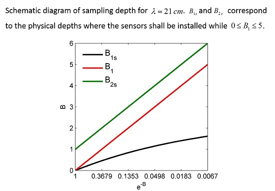
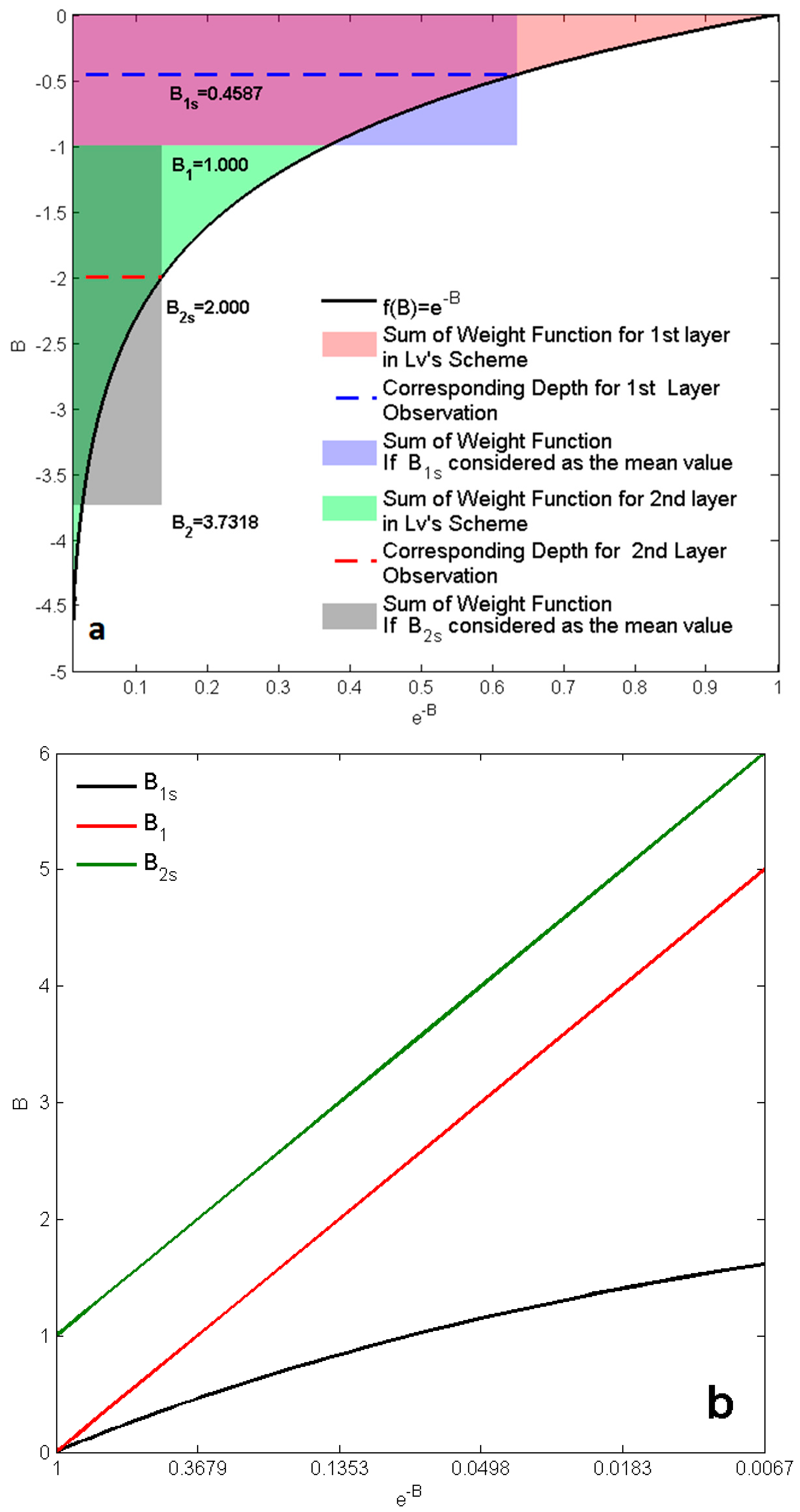
2.1. Characteristics of Parameter B

Lv’s scheme uses an exponential function to distribute the weight among different layers (see Equation (4)). The only parameter in this scheme is $B$, which is another form of $\alpha$ in Wilheit’s scheme. A series of extended concepts used to analyze the characteristics of $B$ are listed in

Table 1. The mathematical details regarding the concepts mentioned in this study.

Name	The First Layer	Middle Layers	The Deepest Layer
$B$	$B_i=\Delta x_i\cdot \frac{4\pi }{\lambda }\cdot \frac{{\epsilon }^{″}}{2\sqrt{{\epsilon }^{\prime }}}$, $\Delta x_i$ is the physical depth interval. Soil moisture/temperature are from the ith layer as well.
Residual $\left(R\right)$	$e^{-B_1}$	${\displaystyle \prod _{j=1}^i{e}^{-B_j}}$	${\displaystyle \prod _{j=1}^n{e}^{-B_j}}$
Weight Function	$1-e^{-B_1}$	$\left(1-e^{-B_i}\right){\displaystyle \prod _{j=1}^{i-1}{e}^{-B_j}}$	${\displaystyle \prod _{j=1}^{n-1}{e}^{-B_j}}$

.

In fact, Lv’s multilayer scheme, which has a general form of exponential terms, is more flexible than the two-layer scheme. To achieve either an assessment of the Maqu Network or a determination of the optimal mounting depth/combination, the multilayer scheme will be deployed. When excluding both the top and bottom layers in the multilayer model, the in-between layers (the ith layer) share a common expression: $T_i\left(1-e^{-B_i}\right){\displaystyle \prod _{j=1}^{i-1}{e}^{-B_j}}$, with $\left(1-e^{-B_i}\right){\displaystyle \prod _{j=1}^{i-1}{e}^{-B_j}}$ called the weight function (double underline in Equation (4)). Thus, the weight function could be further divided into two parts: the representative term $\left(1-e^{-B_i}\right)$, which is dealing with $B$ at the ith layer, and the term ${\displaystyle \prod _{j=1}^{i-1}{e}^{-B_j}}$, which could be computed with $B$ above the ith layer. ${\displaystyle \prod _{j=1}^{i-1}{e}^{-B_j}}$ determines how much weight from the ith layer can directly contribute to $T_{eff}$ without any prior knowledge of the ($i+1$)th layer. In other words, if the ($i+1$)th layer exists, whatever the soil temperature at the ($i+1$)th layer is, the soil temperature at the ($i+1$)th layer has to be multiplied by ${\displaystyle \prod _{j=1}^i{e}^{-B_j}}$. Hence, ${\displaystyle \prod _{j=1}^i{e}^{-B_j}}$ can be called the residual (single–underline in Equation (4)) of the ith layer. With these concepts in mind, it is possible to estimate the potential contributions by different layers when calculating $T_{eff}$, as discussed in Section 3.1.

In the following, the mathematical derivation of Lv’s scheme will be implemented to derive the optimal mounting depth. In Equation (3), $T_1$ depicts the mean soil temperature of the first layer, with $1-e^{-B_1}$ forming its weight in the calculation of $T_{eff}$. The same can be said for the second layer, for $T_2$ and $e^{-B_1}$. It can be inferred that the result will only be optimal if the following conditions are met:

(1)

$T_1$ matches the layer-averaged soil temperature integrated from the surface to the sampling depth $\Delta x$, which is used for calculating $1-e^{-B_1}$ (see Equation (3));

(2)

$T_2$ matches the layer-averaged soil temperature integrated from the sampling depth $\Delta x$ to the infinite, as in Equation (2).

When the above two conditions are met, the weights calculated by Equation (3) are the most representative for the first and second layer, in terms of calculating $T_{eff}$. The representativeness (i.e., depth intervals) of $T$ is clearly defined in numerical model outputs; for instance, 0 to 7 cm for the first layer, 7 to 28 cm for the second layer, 28 to 100 cm for the third layer, and 100 to 289 cm for the bottom layer in ERA-interim reanalysis data. The same concept exists for observation data like the Maqu Network. The question of which depth interval a SM/ST sensor could represent is critical, considering Conditions 1 and 2.

Table 2. The explanation of the parameters used in determining the optimal mounting depths.

B	Δx	Soil Moisture	Soil Temperature
$B_{1s}$	$\Delta x_{1s}$, the mounting depths of sensors in the first layer	The first layer samples	The first layer samples
$B_1$	$\Delta x$, deduced from $1-e^{-B_1}=e^{-B_{1s}}{B}_1$	Layer-averaged (1st layer)	Layer-averaged (1st layer)
$B_{2s}$	$\Delta x_{2s}$, the mounting depths of sensors in the second layer	The second layer samples	The second layer samples
$B_2$	Not necessarily defined	Not necessarily defined	Not necessarily defined

explains the definition of parameters used in determining the optimal mounting depths. To keep consistent with the $B_1$ in Equation (3), $B_{1s}$ and $B_{2s}$ are proposed to stand for the corresponding $B$ values at the mounting depth of $\Delta x_{1s}$ and $\Delta x_{2s}$, where the sensors are installed.

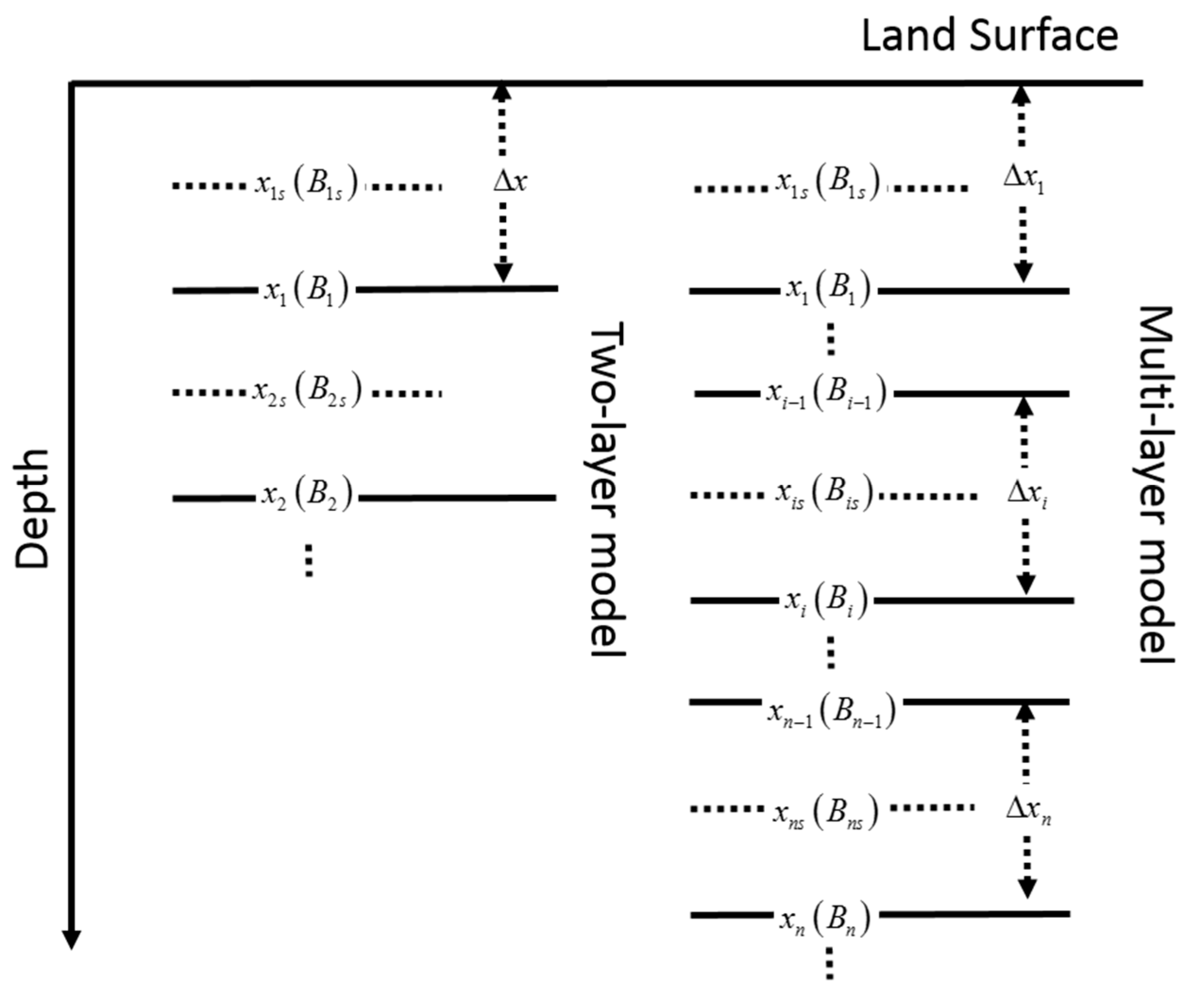
2.2. Optimal Mounting Depth

Considering the integral exponential function ${\displaystyle \int e^{-x}dx=}1-e^{-x}$, it could be deduced that for each layer in soil profile $dx$, its weight should be $e^{-B}$. In order to satisfy Condition 1, the first layer $e^{-B_{1s}}$ is supposed to be the mean value of ${e^B|}_0^{B_1}$, e.g., $e^{-B_{1s}}=\frac{1}{B_1}{\displaystyle {\int }_0^{B_1}{e}^{-B}dB}=\frac{1}{B_1}\left(1-e^{-B_1}\right)$. This demonstrates that the weight $e^{-B_{1s}}$, calculated by using SM/ST at sampling depth $\Delta x_{1s}$, should match the layer-averaged $e^{-B}$. Here $e^{-B_1}$ should be calculated by using the layer-averaged SM/ST with a layer thickness of $\Delta x$.

For the second layer, to satisfy Condition 2, $T_2$ is assumed to match the layer-averaged soil temperature integrated from the interval $\left[B_1,\infty \right]$. The infinite is usually represented numerically by using a cutting-off error with a finite number (in this case: $\infty \approx B_2+cutting\_off\_error$). Consequently, $T_2$ is here defined as the layer-averaged ST between $\left[B_1,B_2\right]$ where $B_1<B_{2s}<B_2$. With a cutting-off error $B_2$, the First Mean Value Theorem for Integration [22] can be applied to prove that there must be a value of $B_{2s}$ that satisfies Condition 2. In fact, $B_2$ can be numerically defined without necessarily being used in the calculation of the subsequent derivation with the math skill introduced below:

The above implies that the weight $e^{-B_{2s}}$ calculated by using the SM/ST at the sampling depth $\Delta x_{2s}$ should match the layer-averaged $e^{-B}$ (e.g., $e^{-B_{2s}}=\frac{1}{\left(B_2-B_1\right)}{{\displaystyle \int }}_{B_1}^{B_2}{e}^{-B}dB\approx \frac{1}{\left(B_2-B_1\right)}{{\displaystyle \int }}_{B_1}^{\infty }{e}^{-B}dB$). Therefore, for the two-layer scheme, the total weight is the sum of

$$\{\begin{array}{l}1-e^{-B_1}=e^{-B_{1s}}{B}_1\\ e^{-B_1}=e^{-B_{2s}}\left(B_2-B_1\right)\end{array}$$

(5)

Since $B_{1s}$ is determined by field observation (e.g., the first SM/ST sensor below the soil surface), Equation (5) contains three unknowns: $B_1$; $B_2$ and $B_{2s}$, but with two formulas. With the preset $B_{1s}$ known, $B_1$ can be calculated by using the first expression in Equation (5). There are two remaining parameters, $B_2$ and $B_{2s}$, that need to be solved in Equation (5).

To meet Condition 2, $T_2$ should match the layer-averaged ST for the second layer, which means $T_2$ is equal to the ST at the sampling depth $\Delta x_{2s}$ (see Table 2), because at this sampling depth the weight $e^{-B_{2s}}$ is representative for the second layer. On the other hand, to be representative for the second layer, the $B_{2s}$ (corresponding to $\Delta x_{2s}$, Table 2) must be located between $B_1$ and $B_2$. Since the First Mean Value Theorem for Integration is defined within a closed interval $\left[B_1,B_2\right]$, an optimal mounting depth of $\Delta x_{2s}$ (e.g., at $\left[B_1,\infty \right]$) has to be determined to enable its layer representativeness. The determination of an optimal mounting depth can be achieved by using the characteristic ratio $\frac{B_2-B_{2s}}{B_{2s}-B_1}$ for the second layer. Expanding this characteristic ratio, considering Equation (5), leads to:

$$\begin{array}{l}\frac{B_2-B_{2s}}{B_{2s}-B_1}=\frac{e^{-B_1}/e^{-B_{2s}}-\left(B_{2s}-B_1\right)}{B_{2s}-B_1}\\ =\frac{e^{B_{2s}-B_1}-\left(B_{2s}-B_1\right)}{B_{2s}-B_1}\end{array}$$

(6)

The form of the function with this characteristic ratio is $f\left(x\right)=\frac{e^x-x}{x}$. Therefore, mathematically, to obtain an optimal characteristic ratio, the first order derivative of $f\left(x\right)$ needs to be equal to zero. There is also a physical meaning: in Figure 2a, as will be discussed, to meet Condition 1 and 2, the pink area has to be made equal to the purple area (i.e., for the first layer), and the green area to the grey area (i.e., for the second layer). As can be seen, if $B_{2s}$ is situated closer to either $B_1$ or $B_2$, the weight of $e^{-B_{2s}}$ will not represent the second layer. Under the precondition that the annual averaged soil temperature tends to be homogeneous throughout the soil profile [23,24,25], to enable the layer representativeness of $B_{2s}$, the difference between $B_2-B_{2s}$ and $B_{2s}-B_1$ has to be made as small as possible. Meanwhile, to enable the grey and the green area to be equal in size for the second layer in Figure 2a, the ratio should not be smaller than a constant, considering the shape of the $f\left(x\right)=\frac{e^x-x}{x}$ curve. To find a solution for $f\left(x\right)$ that reduces the ratio as much as possible actually means the first order derivative of $f\left(x\right)$ should be equal to zero. This leads to $x=1$, for the current function form, which means

$$B_{2s}-B_1=1$$

(7)

In this way, $B_2$ does not need to be defined exactly (Table 2), with the cost of causing a cutting-off error. However, due to the infinite form of Equation (2), the cutting-off error determined by the approach indicated above cannot be 0, but can be infinitely approaching 0. With the relation obtained in Equation (7), Equation (5) may be rewritten as,

$$\{\begin{array}{l}1-e^{-B_1}=e^{-B_{1s}}{B}_1\\ B_{2s}=B_1+1\end{array}$$

(8)

where $B_{1s}=\Delta x_{1s}\cdot \frac{4\pi }{\lambda }\cdot \frac{{\epsilon }^{″}}{2\sqrt{{\epsilon }^{\prime }}}$ is computed by the SM/ST data collected at the first layer in the field experiment ($\Delta x_{1s}=0.05m$ for the Maqu Network). With Equation (8), the determination of $B_1$ is easy in the first expression once $B_{1s}$ is known. This then naturally leads to the determination of $B_{2s}$ in the second expression.

Figure 2a explains the concept of Equation (8) in a schematic diagram, by showing the relationship between the parameter B and the residual $e^{-B}$ in a two-layer $T_{eff}$ model. If the present value $B_1=1$ is used, then $B_{1s}$ and $B_{2s}$ can be derived by using Equation (8). For each B value, a corresponding depth can be calculated by $B_i=\Delta x_i\cdot \frac{4\pi }{\lambda }\cdot \frac{{\epsilon }^{″}}{2\sqrt{{\epsilon }^{\prime }}}$, where SM/ST is measured for each layer at the sampling depth of $\Delta x_i$. Therefore, the explanation of physical depth $\Delta x$ is tied up with $B$. This relationship may be expressed as $B=g\left(\Delta x\right)$. According to Equation (8), if the first layer sensor is installed at $\Delta x_{1s}$, this will correspond with $B_{1s}$, while the depth interval $\Delta x$ should correspond with $B_1$ (e.g., layer-averaged). Then, to meet Condition 1, the pink area should be equal to the purple area in Figure 2a.

After determining $B_1\left(\Delta x\right)$, the remaining area (i.e., the green area) represents the weight given to the second layer, from which $B_{2s}\left(\Delta x_{2s}\right)$ can be inferred. The ratio (e.g., $B_1/B_{1s}$, $B_{2s}/B_{1s}$) obtained by Equation (8) can be used to infer the optimal mounting depth, if the thickness of the first layer is fixed. For instance, if $B_{1s}$ obtained from this ratio is 0.46, which corresponds to a sampling depth of $\Delta x_{1s}$, then $B_1$ is assumed to equal 1. Furthermore, $B_{2s}$ should equal 2, based on Equation (8), and this corresponds to another sampling depth, $\Delta x_{2s}$. Figure 2a and Equation (8) both indicate the capability of Lv’s scheme in identifying the optimal mounting depth. They are deemed the simplified form of the multilayer model described in Equation (4).

Figure 2b mathematically shows $B_{1s}$, $B_1$ and $B_{2s}$ distributed in a “$Bvs.e^{-B}$” domain, based on Equation (8). As discussed above, with a sensor positioned at a certain mounting depth, the “$B vs. e^{-B}$” domain can help to understand how the weight of the soil layer at that depth contributes to the calculation of $T_{eff}$. By assuming $B_{1s}$ = 0, 1, 2, …, we can obtain the black line in Figure 2b. Furthermore, $B_1$ is a function of $B_{1s}$($B_1=f\left(B_{1s}\right)$) and $B_{2s}$ is a function of $B_1$. Therefore, with $B_{1s}$ varying, $B_1$ and $B_{2s}$ form curves, as shown in Figure 2b. It should be noted that the y-axis in Figure 2b indicates a special case: if there is only one layer left to represent the whole soil volume, then $B_{2s}=1$ is the optimal option. In this case, the real optimal mounting depth ($\Delta x_{2s}$) could be inferred from $B_{2s}=1=\Delta x_{2s}\cdot \frac{4\pi }{\lambda }\cdot \frac{{\epsilon }^{″}}{2\sqrt{{\epsilon }^{\prime }}}$, considering the SM/ST conditions for dielectric constant. It is coincidental with the concept of penetration depth or what is called the temperature sensing depth as that depth satisfies $1/e$ of Equation (2) [26,27]. The distribution of curves in Figure 2b is generic, and the curves are characteristic and derived from Equation (8). Figure 2a can be seen as a single vertical cross-section of Figure 2b. With Figure 2b, it is possible to identify the optimal mounting depth $\Delta x_i$ (i = 1, 2), as long as $B_{1s}$ and $B_{2s}$ computed from specified ST/SM profiles align with the black and the green reference lines, respectively. As long as computed $B_{1s}$ and $B_{2s}$ meet the reference lines, Equation (8) is satisfied. To sum up, the basic steps in determining the optimal sampling depth could be:

(1)

Using SM/ST observation at first layer ($\Delta x_1$) to calculate $B_{1s}$ with $B_i=\Delta x_i\cdot \frac{4\pi }{\lambda }\cdot \frac{{\epsilon }^{″}}{2\sqrt{{\epsilon }^{\prime }}}$;

(2)

Using $B_{1s}$ to calculate $B_1$ and $B_{2s}$ with Equation (8);

(2)

Determining the optimal sampling depth for the second layer with $B_i=\Delta x_i\cdot \frac{4\pi }{\lambda }\cdot \frac{{\epsilon }^{″}}{2\sqrt{{\epsilon }^{\prime }}}$ again.

If a network already exists whose sensors are installed at several depths ($\Delta x_i$), then select a two-layer combination and calculate its $B_{1s}$ and $B_{2s}$. The pair of $B_{1s}$ and $B_{2s}$ that fits Equation (8) is the optimal sampling depth. The application of Figure 2b to an existing network (Maqu Network) will be discussed in Section 3.2.

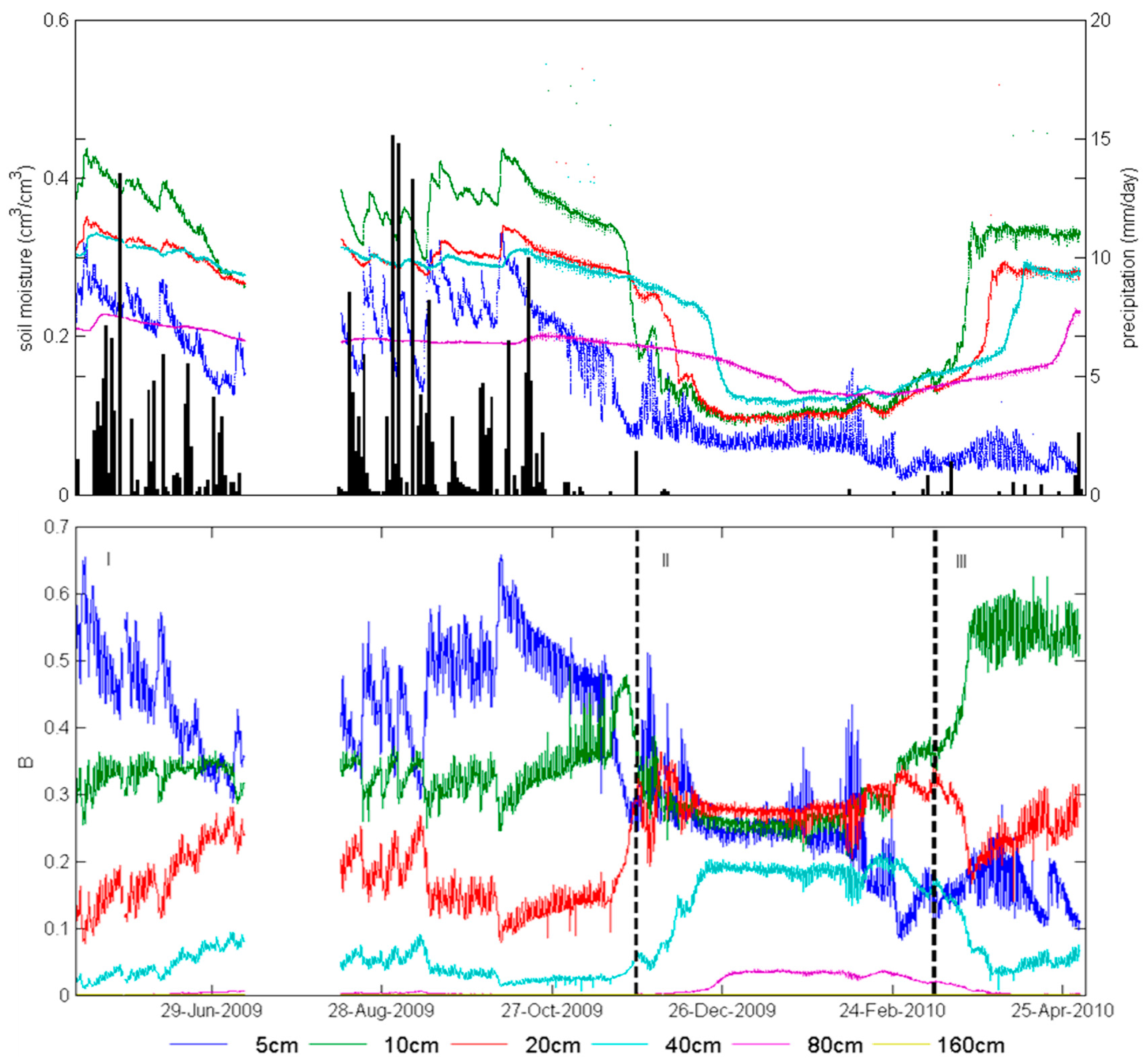
2.3. The Maqu Network

In 2008, a soil moisture monitoring network was set up at Maqu [28,29]. Maqu is located in the source region of the Yellow River and the east margin of the Tibetan Plateau. The average elevation is around 3300 m above sea level. The vegetation consists of alpine shrublands and meadows, with grasses less than 1 meter in height with roots extending tens of centimeters in depth. An accumulated humus layer of around 10 cm is mixed with the soil. Shrubs and trees are scarce in this region, while desert dunes sometimes appear along the river. The network includes 20 sites with a variety of terrain and soil textures, such as silt loam and sandy loam. The observation depth is set to 5 cm/10 cm for most sites, but a few sites have enhanced layer settings of 20 cm, 40 cm and 80 cm, respectively. Three of these sites, C01, N01 and N02, are relatively close to each other, i.e., within 200 m. There is also a boundary layer meteorological tower at C01, which takes its own SM/ST measurements; this station is hereafter called the center station [30]. The layer settings for the center station are 5 cm, 10 cm, 20 cm, 40 cm, 80 cm and 160 cm, with an additional infrared sensor for the skin temperature. Since its establishment, the Maqu Network has provided accurate soil parameters for retrieving soil moisture data from satellites at the L-band [30,31,32,33]. The time series of SM/ST at center station were collected from May 2009 to April 2010. To avoid introducing the additional complexity of frozen soil, the calculation in Section 3.2 is based only on the time series where ST > 0. Additionally, to obtain $T_{eff}$ time series via the Wilheit’s scheme, the Noah Land surface model [28] was adopted to generate ST/SM profiles with 37 layers (0 to 500 cm) between 12 and 28 June 2010.

3 Results

3.1. Evaluation of Installation Configuration

The spatial resolution of passive microwave radiometers on satellite platforms is coarse compared to an area, which could be represented by a single SM/ST site. For instance, SMOS produce brightness temperature observation data with a resolution of about 40 km on average [11]. For the whole region covered by the Maqu Network, $T_{eff}$ calculated from a single site is not representative enough considering the degree of spatial variability in soil moisture and texture. It is common practice to take the average value for all sites in the network and compare this to the brightness temperature observation produced. Usually, the arithmetical average is used. In this section, the $B$ values (i.e., weights) for different layers at the center station will be calculated using Equation (4). The same method can be applied over the whole network. How to evaluate the reliability of a single site, in terms of accurately evaluating $T_{eff}$, will be discussed in this section. The center station will be used as an example first and then the discussion will extend to other sites in the Maqu Network. The consecutive mounting depths employed at the center station are 5, 10, 20, 40, 80 and 160 cm.

Figure 3 shows the time series for $B$ values (e.g., the contribution of weight, Table 1) at different mounting depths (or layers) at center station. The time series is divided into three periods: April to November 2009; November 2009 to February 2010; and the period after February 2010. The valley-shaped curve (e.g., for the upper layers ≤20 cm) for the second period might be explained by the soil being frozen (when soil temperature is below 0 °C). Frozen soil makes the SM/ST profile homogenous, which leads to similar B values for the upper layers (≤40 cm). Usually, the upper layer contributes most to the $T_{eff}$, as seen in the first period. However, this is not the case in the third period. The contribution from the 10 cm layer is dominant in the third period. This implies that a two-layer model, which considers only the 5 cm and 160 cm layers, for instance, may lead to significant errors (e.g., loss of signal from the 10 cm layer).

As expected, $B$ varies throughout the seasons [20]. However, the variation is not induced by an inter-annual cycle, but corresponds strongly to soil moisture. Several rainfall events can be identified that increased soil moisture at 5 cm and subsequently the $B$ values for that same layer. However, the other layers (10, 20, 40, 80, and 160 cm) demonstrate different characteristics and may even be opposite phases to those at 5 cm. The $B$ values of the 5 cm and the 10 cm layer show opposing patterns (the blue and green lines for Period I and III in Figure 3). The reduction of $B$ at 5 cm, for Period III, is caused by surface dryness and lack of rainfall (e.g., soil moisture is less than 0.05 $c{m}^3\cdot c{m}^{-3}$ at 5 cm). On the other hand, the mean soil moisture content at 10 cm at that time is around 0.35 $c{m}^3\cdot c{m}^{-3}$.

Figure 4 indicates the time series of the residual (see definition in Table 1) for all layers. During Period I, when calculating $T_{eff}$, about 50% of the weight comes from the soil layer 0 to 5 cm (blue line in Figure 3), while the other 50% originates from the soil layers below 5 cm (i.e., the residual, Figure 4). The soil layer at 10 cm will contribute about 30% of the weight in calculating $T_{eff}$ (green line in Figure 3). The remaining 20% of the weight will be derived from the soil layers below 10 cm (red line and rest in Figure 4). Thus, the soil layers at 5 cm and 10 cm combined will contribute about 80% of the signal when estimating $T_{eff}$ at the center station. If we include more layers in the calculation, more weight will be included. For example, if information from the 20 cm layer is also included, only the 5% of weight from the soil layers beneath the 20 cm layer will not be considered.

During Period II, the soil is frozen, which makes the soil column vertically homogenous. The dielectric behavior of frozen soil is similar to dry soil; hence, the penetrating depth increases, which means that the microwave emission reaching the surface may come from deeper soil layers, implying an increased residual for each soil layer. In Figure 4, it can be seen that in Period II all residuals are increased, compared to other periods.

During Period III, the weight from the first layer (i.e., 5 cm) may be greatly reduced, but here the 10 cm layer might contribute more than 60% (green line in Figure 3). Correspondingly, during this period, by taking 5 cm as the corresponding depth in the first layer, the residual of weight is greatly increased (e.g., to be about 80%, blue line in Figure 4). On the other hand, the residual of weight for the 10 cm layer drops dramatically, to less than 30%, since the inclusion of the 10 cm increases the upper layer’s contribution in the calculation of $T_{eff}$.

To sum up, it can be inferred that considering only the weight contribution from the combination of 5 cm and 10 cm (Figure 3 and Figure 4) is not enough to estimate $T_{eff}$ accurately, as the total represented weight will be only about 80%. If the 20 cm weight is also taken into account, the total weight will be around 90%, even without considering the contribution from 40 cm, 80 cm, and 160 cm. Thus, the calculation of parameter B (i.e., the weight contribution or the residual weight) may be applied to assess how representative each site in the Maqu Network is when estimating $T_{eff}$.

It can be inferred that, in order to estimate $T_{eff}$ as accurately as possible, the physical mounting depth should be designed to minimize the residual as much as possible. To provide a proof of concept calculation, the same mounting depth was used throughout the Maqu Network, with $\Delta x_1=5 cm$ for the first layer and $\Delta x_2=10 cm$ for the second layer. For each site, the residual of weight for the second layer (${\displaystyle \prod _{j=1}^1{e}^{-B_j}}$, the middle layer as in Table 1) is shown in blue bars, while green bars represent the third layer (${\displaystyle \prod _{j=1}^2{e}^{-B_j}}$, the deepest layer as in Table 1, Figure 5). The smaller residual signal in Figure 5 indicates the smaller error of each site in estimating $T_{eff}$. Figure 5 shows that the NST-04 site is relatively reliable, with an error in estimating $T_{eff}$ of less than 10%. This means that, based on the 5 cm and 10 cm installation configuration, the NST-04 site can be used to calculate $T_{eff}$ representatively, especially when compared to other sites in the Maqu Network (Figure 5). Similarly, the NST-09 site is found not to be suitable for calculating $T_{eff}$, as the residual weight from the other soil layers can be about 40%, thus contributing to 40% of the error when estimating $T_{eff}$. Therefore, the NST-09 site should be given less credit when looking for a spatial average. There are many ways to choose the representative sites based on statistics like the Optimal Selection of Alteration Information Extraction Method. However, for the L-band, the pixel could be tens of kilometers, which means that all sites within the Maqu Networks make a contribution to the final signal detected by SMOS/SMAP. None of the sites could be simply removed or given full credit (weight number = 1) because of the complexity of soil moisture profiles, etc. The arithmetical average is taken for this reason, usually because of a lack of physical criteria. The basic hypothesis here is that the uncertainty (residual) is related to the weight. No site is removed or perfect, rather it is given a relative reliability among all sites. To quantify this credit $\left(C\right)$, the use of the normalized residual signal is suggested, to be expressed as:

$$C_i=1-\frac{R_i-R_{\min }}{R_{\max }-R_{\min }}$$

(9)

where $i$ represents the ith site, i = 1 to n (i.e., the total number of sites in a network); $R_{max}$ and $R_{min}$ represent the maximum and minimum residual among all sites. Then, for the Maqu Network, an averaged value of $T_{eff}$ could be given by

$$T_{eff}=\frac{{\displaystyle \sum _{i=1}^n{T}_{effi}\times C_i}}{{\displaystyle \sum _{i=1}^n{C}_i}}$$

(10)

where $T_{eff}$ represents $T_{eff}$ calculated at the ith site with the 5 cm and 10 cm installation configuration. It is important to use Equations (9) and (10) to obtain an area-averaged $T_{eff}$. The measurement configuration will be optimal only when the residual approaches 0. None of the sites in the Maqu Network is less than 0.2, while the larger values imply a deficiency of instrument installation in describing $T_{eff}$. Without using these two equations on average at least 20% of $T_{eff}$ signals cannot be captured by the Maqu Network with this assumed sensor installation configuration (5 cm & 10 cm). This approach is generic and can be applied to other observation networks to evaluate their representativeness in estimating $T_{eff}$.

Theoretically, according to Equation (2), $T_{eff}$ will vary daily and seasonally with the SM/ST profiles and the mounting depth will vary as well. Nevertheless, the mounting depths of the SM/ST sensors are fixed once they are installed. For most of the sites in the Maqu Network, 5 cm/10 cm is a default installation setting for measuring SM/ST. Whether the 5 cm/10 cm combination is optimal for estimating effective temperature has not yet been discussed. It is clear that there is no fixed depth configuration that can accommodate all variations in SM/ST throughout the year for obtaining a perfect estimation of $T_{eff}$ variation. However, according to the in situ installation configuration, it is possible to investigate what the optimal mounting depth is in order to approach the perfect estimate of $T_{eff}$. A practical way is to find the optimal combination of sensor installations that will represent the mean SM/ST for that site. The center station will be used as an example of such an investigation. The same procedure can then be applied across the whole Maqu Network.

3.2. Test of the Optimal Mounting Depth

The section above discusses how the residual weight can be estimated by Lv’s scheme. This section will describe how to determine the optimal mounting depth. Based on this discussion, the current installation configuration at the Maqu Network can be enhanced by adding sensors to the current configuration according Lv’s scheme.

For the field experiment, it is important to have a method to arrive at the optimal installation configuration. The proposed approach in this study is as follows: firstly, a defined depth is given to the top layer (i.e., $\Delta x_{1s}$), e.g., two columns with black squares in Figure 6a, 5 cm and 10 cm; and secondly, using Equation (8), $B_1$ may be calculated and the depth for the second layer determined (i.e., $\Delta x_{2s}$). Two columns are shown to present two different cases of study: (1) the first layer at the Maqu Network is 5 cm (marked in text) and $B_{5 cm}$ = 0.267 (y-axis) and assumes 20 cm/40 cm/80 cm/160 cm to be the second layer; 10 cm is not shown because $\Delta x>10 cm$ (Table 2) when 5 cm is the first layer; (2) the first layer at the Maqu network is 10 cm and $B_{0.1m}$ = 1.268 and assumes 40 cm/80 cm/160 cm to be the second layer; 20 cm is not included for the same reason noted above. With the same technique, we acquired the positions of all other layers (indicated by asterisks with the depth information). Not all layers deeper than the assumed first layer could be the second layer because according to Equation (8), $\Delta x$ may be larger than the supposed second layer. For instance, when 5 cm is the first layer, $\Delta x=11.8 cm$ which is bigger than 10 cm. It is not necessary to take 10 cm into consideration since most of its information could be represented by 5 cm. This approach has been utilized to plot Figure 2b. The existing sites already have a fixed $\Delta x_1$ (therefore a fixed $B_{1s}$) for the first layer. Thus, $B_1$ can be easily calculated here using Equation (8). The core concept is that the choice of depth combination (e.g., 5 cm and 10 cm, or 5 cm and 20 cm, etc.) reduces the residual to a minimum (e.g., ideally = 0) under the constraint of Equation (8). The data collected at the center station contain six layers of SM/ST observations, which will be used to show which two of these layers can best estimate $T_{eff}$. The similar approach can be applied at other sites in the Maqu Network.

According to Equation (8), based on the installation depth and the associated mean SM/ST, the sensor installation configuration can be mapped on the “$B vs e^{-B}$” domain as well (Figure 6). The observations at 5 cm, 10 cm, 20 cm, 40 cm, 80 cm, and 160 cm depth at the center station were plotted in this way and pooled in Figure 6a. The $B_1$ curve (corresponding to $\Delta x$) divides the soil column into two parts. The $B_{1s}$ curve indicates that the $-B$ (y-axis) and residual for the second layer $e^{-B}$ (x-axis) can be achieved if a sensor is installed at $\Delta x_{1s}$, and the $B_{2s}$ curve indicates $-B$ for $\Delta x_{2s}$ while the first layer determines $e^{-B}$. Figure 2b shows that the $B_{1s}$, $B_1$ and $B_{2s}$ curves are derived directly from Equation (8), which is generic and independent of mounting depth and SM/ST information. This implies that if the sensor installation configuration is mapped in the “$B vs e^{-B}$” domain, it can have matching points with the $B_{1s}$ and $B_{2s}$ curves. Then the corresponding installation configuration can be deemed the optimal configuration (or the optimal mounting depths). In other words, if the sensors can be installed at mounting depths corresponding to the $B_{1s}$ and $B_{2s}$ lines, the residual calculated from such an installation configuration would be minimized and the mounting depths considered optimal. For the center station, two pairs of lines emerge (Figure 6a): 5 cm and 20 cm, as well as 10 cm and 40 cm. From Figure 6a it can be deduced that the second pair contributes less than 5% to the $T_{eff}$ calculation (x-axis, $e^{-B_1}<0.05$). Therefore, the optimal mounting depths are 5 cm and 20 cm for the center station of the Maqu Network. The same strategy can be used at the other sites in the Maqu Network, which have sensors installed at 5 cm/10 cm/20 cm/40 cm or 5 cm/10 cm/20 cm/40 cm/80 cm (Figure 6b).

Assuming Wilheit’s scheme provides the true value,

Table 3. Correlation coefficient and RMSE with available six-layer soil moisture/soil temperature profiles.

Configuration	5 cm/10 cm	5 cm/20 cm	5 cm/40 cm	5 cm/80 cm	5 cm/160 cm	10 cm/20 cm	10 cm/40 cm	10 cm/80 cm
Residual $\left(R\right)$	0.311	0.074	0.039	0	~	0.034	0.002	≈0
Weight function for the first layer $1-e^{-B_1}$	0.496	0.496	0.496	0.496	0.496	0.950	0.950	0.950
$B_{2s}-B_1$	−0.067	0.943	2.907	5.367	10.442	−0.610	1.374	4.168
Correlation Coefficient	0.9951	0.9981	0.9900	0.9700	0.9572	0.9876	0.9884	0.9880
RMSE(K)	0.93	0.44	1.12	1.77	2.46	1.09	1.02	1.05

compares the possible combinations of layer pairs at the center station for calculating $T_{eff}$. This confirms that the optimal mounting depths are 5 cm and 20 cm and that this combination performs best when estimating $T_{eff}$. The residual of the 5 cm and 10 cm combination is 0.311 which means 31.1% of the $T_{eff}$ signal beneath is unknown and implies potential uncertainty. The same information is deduced from Figure 4 and Figure 5, where the residuals of all sites are compared. Most combinations arrive at a small residual but only the 5 cm and 20 cm and the 10 cm and 40 cm combinations meet the $B_{2s}-B_1=1$ rule. It may be inferred that if the first layer is fixed at 10 cm, it is impossible to reach good agreement, since the representative term $\left(1-e^{-B_1}\right)$ for the 10 cm layer is more than 95% with only 5% left for the second layer (i.e., the first layer is set too deep to represent the top layer information, which will lead to the underestimation of $T_{eff}$). The SM/ST information near the surface is overwritten by the 10 cm. In this case, the accuracy of output from Lv’s scheme cannot be guaranteed. To summarize, the 5 cm and 20 cm combination has proven to be the best combination used as input for Equation (3). More importantly, this realization can be deduced mathematically from Equation (8) as discussed in Section 2.

To apply Wilheit’s integral $T_{eff}$ scheme, the minimum number of soil layers should be more than 20 [34]. Therefore, an extra-intensive model investigation of SM/ST was done for the period from 12 to 18 June 2010 and was simulated using the Noah Land-surface model. The total number of layers used is 37, from the soil surface to 5 m deep. Of these layers, 25 are within the upper 1 meter, which guarantees that an accurate $T_{eff}$ will be acquired as the reference value by applying Wilheit’s integral equation. With these 37 layers, all combinations of two different layers are used to generate a $T_{eff}$ time series by the method of exhaustion, and then the reference value is compared with RMSE, as shown in Figure 7. For instance, the blue line with squares stands for the case where the first layer is 0.25 cm. The first square from the left in this blue line is the combination of 0.25 and 0.5 cm, the second one is 0.25 and 1 cm, the third is 0.25 and 2 cm, etc. The solid line with squares stands for a fixed first layer mounting depth and the dash line with crosses for the RMSE variation along with the changing second layer mounting depth. It demonstrates that if the first mounting depth is shallow, the best $T_{eff}$ estimation can only be achieved when $B_{2s}-B_1=1$ (for the lines from 0.25 cm to 5 cm in Figure 7). Conversely, RMSE will increase dramatically if the first mounting depth is very deep (regardless of the second mounting depth). For the period in Figure 7, the optimal combination of mounting depths is 3 cm and 14 cm because it reaches the lowest RMSE (the black line with black square stands for 3 cm and the 9th square counting from the left stands for 14 cm). Figure 7 also proves that with the appropriately configured mounting depth, $T_{eff}$ accuracy can be improved by at least several Kelvins. As indicated earlier, this combination is suitable only for the simulated period. To find the optimal mounting depth at the center station for the whole year, the annual mean SM/ST values from the existing mounting layer are needed. For the Maqu Network, the same principle seen in Equation (8) shows that the second mounting depth should be around 20 to 25 cm (with different dielectric mixing models) instead of the current 10 cm, with a mean SM = 0.138 $c{m}^3/c{m}^3$ and ST = 4.503 °C. In addition, the penetration depth/temperature sensing depth is also seen in Figure 7 because some lines (the lines with cross marks) could also reach nearly the minimum RMSE while $B_1$ ($B_{1s}$) is fixed. In these lines, RMSE does not increase with $B_{2s}$. It means $B_{1s}\approx 1$ and the first mounting depth already accounts for most of the weight for calculating $T_{eff}$.

4. Discussion

Either the definition of residual or the relationship of optimal mounting depth derived in this study is based on Lv’s soil effective temperature scheme and its parameter $B$($B=\Delta x\cdot \frac{4\pi }{\lambda }\cdot \frac{{\epsilon }^{″}}{2\sqrt{{\epsilon }^{\prime }}}$). The essence of $B$ is a thickness of medium where the energy is reduced to $1/e^B$ of its original (emitted) value. This is in coincidence with the concept of the sensing or penetrating depth in remote sensing when $B=1$. In this case, Wilheit’s integral $T_{eff}$ scheme could be expressed as $T_{eff}={\displaystyle {\int }_0^{\infty }T\left(\tau \right)d{e}^{-\tau }}$, where $\tau =B$. The residual could be comprehended as the percentage of energy which is not captured by existing ST/SM observation when used directly in microwave remote sensing. Similarly, the optimal mounting depth is a description of the mounting depths of two sensors in view of an optical thickness that corresponds to the microwave wavelength.

The main difficulty of these two methods is due in part to the definition of parameter $B$ which assumes the SM/ST is constant or has only a linear gradient within one fixed layer. This assumption is only an approximation and is not always true, especially when it is under extreme dry environment [35,36]. The extent to which this assumption is satisfied depends on how many layers are involved. This is the same reason why Lv’s multi-layer scheme approaches Wilheit’s integral scheme as the number of layers increases. Furthermore, it is not surprising that in Figure 2b, if there is only one layer left then $B_{2s}=1$ is the optimal mounting depth because $1/e$ is the penetration depth, also known as the soil temperature sensing depth. The soil temperature observed at the soil temperature sensing depth equals $T_{eff}$ if the variation of ST is linear.

Potentially, the Lv scheme could be applied to the frozen/thaw study as well. Seen from Figure 3, the B character is strongly affected by the frozen/thaw events during the transfer period from Period I to Period II. However, the soil moisture detected by the sensors in field becomes vertical uniform values when the soil temperature drops below 0 °C. In this study, it seems the freeze/thaw signal could be captured by B parameter. It means the $T_{eff}$ can capture the emission signal even during freezing/thawing process. For the same reason, with complex dielectric model which considers water-ice mixing case, $T_{eff}$ calculation is possible and may be further applied to $T_B$ simulation at L-band over frozen ground.

5. Conclusions

As stated in the introduction, there are many networks around the world for calibrating and validating soil moisture retrieval from microwave satellite observations. The representativeness of these SM/ST observing networks for calculating $T_{eff}$ and in particular, their in situ sensor configuration can be evaluated by the method developed in this study. The operational SMOS retrieval uses the ECMWF simulated global soil temperatures of the first layer and either the deepest or next-deepest layer, as the surface and deep temperature, respectively. Wigneron’s two-layer $T_{eff}$ scheme took this pair of soil temperatures as inputs with auxiliary information [11]. Similarly, the SMAP retrieval assumes a homogenous soil temperature and soil moisture profile at 6:00 A.M. and 6:00 P.M. and uses the surface skin temperature and soil temperature at 0–10 cm from the MERRA-Land model as the surface and deep temperature, respectively [36,37]. The arithmetical average of these two temperatures is taken as $T_{eff}$. This study illustrates how to use Lv’s scheme in assessing the Maqu Network, in terms of identifying the optimal mounting depths for a representative calculation of $T_{eff}$. With better installation configurations, more accurate estimates of $T_{eff}$ can be achieved and the soil moisture remote sensing product can be improved.

The main conclusions of this paper are: (1) Lv’s scheme can be used to assess which site has relatively reliable and sufficient information for estimating $T_{eff}$ accurately. Section 3.1 showed that on average 20% of the signal is lost with the default 5 cm/10 cm installation configuration. Relatively speaking, the NST-09 site should be given little credit and the NST-04 site more credit in calculating the spatial average $T_{eff}$ value, as indicated by Equations (9) and (10); (2) Lv’s scheme determined that the 5 cm/20 cm depth combination is the best configuration for the center station of the Maqu Network. Both mathematically and physically, it is proven that the second layer should be installed at 20 cm instead of at 10 cm at the center station in the Maqu Network. A similar approach may be applied to determine the optimal installation configuration for other monitoring networks, which can contribute to a homogenized validation strategy [38] for satellite soil moisture products. By using the newly developed Lv’s scheme, it will be feasible to determine which layer of soil moisture can be detected by the radiometer. This could be useful in improving the capacity of in situ monitoring networks to calibrate and validate satellite soil moisture observations over different climate zones. It can also be used to derive the actual soil depths of the retrieved soil moisture and estimate the related errors, thus providing additionally important information for applications (e.g., in data assimilation).

References

1. Su, Z.; de Rosnay, P.; Wen, J.; Wang, L.; Zeng, Y. Evaluation of ECMWF’s soil moisture analyses using observations on the Tibetan Plateau. J. Geophys. Res. Atmos. 2013, 118, 5304–5318. [Google Scholar] [CrossRef]
2. Van den Hurk, B.; Best, M.; Dirmeyer, P.; Pitman, A.; Polcher, J.; Santanello, J. Acceleration of land surface model development over a decade of glass. Bull. Am. Meteorol. Soc. 2011, 92, 1593–1600. [Google Scholar] [CrossRef]
3. Seneviratne, S.I.; Corti, T.; Davin, E.L.; Hirschi, M.; Jaeger, E.B.; Lehner, I.; Orlowsky, B.; Teuling, A.J. Investigating soil moisture-climate interactions in a changing climate: A review. Earth Sci. Rev. 2010, 99, 125–161. [Google Scholar] [CrossRef]
4. Koster, R.D.; Suarez, M.J.; Higgins, R.W.; Van den Dool, H.M. Observational evidence that soil moisture variations affect precipitation. Geophys. Res. Lett. 2003, 30. [Google Scholar] [CrossRef]
5. Zhang, J.Y.; Wu, L.Y.; Dong, W.J. Land-atmosphere coupling and summer climate variability over East Asia. J. Geophys. Res. Atmos. 2011, 116. [Google Scholar] [CrossRef]
6. Overpeck, J.T. Climate science: The challenge of hot drought. Nature 2013, 503, 350–351. [Google Scholar] [CrossRef] [PubMed]
7. Kim, J.-E.; Hong, S.-Y. Impact of soil moisture anomalies on summer rainfall over East Asia: A regional climate model study. J. Clim. 2007, 20, 5732–5743. [Google Scholar] [CrossRef]
8. Santanello, J.A.; Peters-Lidard, C.D.; Kumar, S.V. Diagnosing the sensitivity of local land-atmosphere coupling via the soil moisture-boundary layer interaction. J. Hydrometeorol. 2011, 12, 766–786. [Google Scholar] [CrossRef]
9. Frye, J.D.; Mote, T.L. Convection initiation along soil moisture boundaries in the southern great plains. Mon. Weather Rev. 2010, 138, 1140–1151. [Google Scholar] [CrossRef]
10. Van den Hurk, B.; van Meijgaard, E. Diagnosing land-atmosphere interaction from a regional climate model simulation over West Africa. J. Hydrometeorol. 2010, 11, 467–481. [Google Scholar] [CrossRef]
11. Kerr, Y.H.; Waldteufel, P.; Richaume, P.; Wigneron, J.P.; Ferrazzoli, P.; Mahmoodi, A.; Al Bitar, A.; Cabot, F.; Gruhier, C.; Juglea, S.E.; et al. The smos soil moisture retrieval algorithm. IEEE Trans. Geosci. Remote Sens. 2012, 50, 1384–1403. [Google Scholar] [CrossRef]
12. Panciera, R.; Walker, J.P.; Kalma, J.D.; Kim, E.J.; Saleh, K.; Wigneron, J.P. Evaluation of the SMOS L-MEB passive microwave soil moisture retrieval algorithm. Remote Sens. Environ. 2009, 113, 435–444. [Google Scholar] [CrossRef]
13. Wigneron, J.P.; Schwank, M.; Baeza, E.L.; Kerr, Y.; Novello, N.; Millan, C.; Moisy, C.; Richaume, P.; Mialon, A.; Al Bitar, A.; et al. First evaluation of the simultaneous SMOS and ELBARA-II observations in the Mediterranean region. Remote Sens. Environ. 2012, 124, 26–37. [Google Scholar] [CrossRef]
14. Wigneron, J.P.; Chanzy, A.; Kerr, Y.H.; Lawrence, H.; Shi, J.C.; Escorihuela, M.J.; Mironov, V.; Mialon, A.; Demontoux, F.; de Rosnay, P.; et al. Evaluating an improved parameterization of the soil emission in L-MEB. IEEE Trans. Geosci. Remote Sens. 2011, 49, 1117–1189. [Google Scholar] [CrossRef]
15. England, A.W. Thermal microwave emission from a scattering layer. J. Geophys. Res. 1975, 80, 4484–4496. [Google Scholar] [CrossRef]
16. Wigneron, J.P.; Kerr, Y.; Waldteufel, P.; Saleh, K.; Escorihuela, M.J.; Richaume, P.; Ferrazzoli, P.; de Rosnay, P.; Gurney, R.; Calvet, J.C.; et al. L-band microwave emission of the biosphere (L-MEB) model: Description and calibration against experimental data sets over crop fields. Remote Sens. Environ. 2007, 107, 639–655. [Google Scholar] [CrossRef]
17. Holmes, T.R.H.; de Rosnay, P.; de Jeu, R.; Wigneron, R.J.P.; Kerr, Y.; Calvet, J.C.; Escorihuela, M.J.; Saleh, K.; Lemaitre, F. A new parameterization of the effective temperature for l band radiometry. Geophys. Res. Lett. 2006, 33. [Google Scholar] [CrossRef]
18. De Rosnay, P.; Wigneron, J.; Holmes, T.; Calvet, J. Parameterizations of the effective temperature for L-band radiometry. Inter-comparison and long term validation with SMOSREX field experiment. In Thermal Microwave Radiation-Applications for Remote Sensing; Mätzler, C., Rosenkranz, P.W., Battaglia, A., Wigneron, J.P., Eds.; IET Electromagnetic Waves Series 52; The Institution of Engineering and Technology: London, UK, 2006; pp. 312–323. [Google Scholar]
19. Wilheit, T.T. Radiative-transfer in a plane stratified dielectric. IEEE Trans. Geosci. Remote Sens. 1978, 16, 138–143. [Google Scholar] [CrossRef]
20. Lv, S.; Wen, J.; Zeng, Y.; Tian, H.; Su, Z. An improved two-layer algorithm for estimating effective soil temperature in microwave radiometry using in situ temperature and soil moisture measurements. Remote Sens. Environ. 2014, 152, 356–363. [Google Scholar] [CrossRef]
21. Mironov, V.L.; Dobson, M.C.; Kaupp, V.H.; Komarov, S.A.; Kleshchenko, V.N. Generalized refractive mixing dielectric model for moist soils. IEEE Trans. Geosci. Remote Sens. 2004, 42, 773–785. [Google Scholar] [CrossRef]
22. Bancerek, G. The fundamental properties of natural numbers. Formaliz. Math. 1990, 1, 41–46. [Google Scholar]
23. Zeng, Y.J.; Wan, L.; Su, Z.B.; Saito, H.; Huang, K.L.; Wang, X.S. Diurnal soil water dynamics in the shallow vadose zone (field site of China University of Geosciences, China). Environ. Geol. 2009, 58, 11–23. [Google Scholar] [CrossRef]
24. Zeng, Y.; Su, Z.; Wan, L.; Yang, Z.; Zhang, T.; Tian, H.; Shi, X.; Wang, X.; Cao, W. Diurnal pattern of the drying front in desert and its application for determining the effective infiltration. Hydrol. Earth Syst. Sci. 2009, 13, 703–714. [Google Scholar] [CrossRef]
25. Hillel, D. Introduction to Environmental Soil Physics; Academic Press: Cambridge, MA, USA, 2003. [Google Scholar]
26. Owe, M.; Van de Griend, A.A. Comparison of soil moisture penetration depths for several bare soils at two microwave frequencies and implications for remote sensing. Water Resour. Res. 1998, 34, 2319–2327. [Google Scholar] [CrossRef] [Green Version]
27. Ulaby, F.T.; Moore, R.K.; Fung, A.K. Microwave Remote Sensing Active and Passive-Volume III: From Theory to Applications; Artech House, Inc.: Dedham, MA, USA, 1986. [Google Scholar]
28. Zheng, D.; van der Velde, R.; Su, Z.; Booij, M.J.; Hoekstra, A.Y.; Wen, J. Assessment of roughness length schemes implemented within the noah land surface model for high-altitude regions. J. Hydrometeorol. 2014, 15, 921–937. [Google Scholar] [CrossRef]
29. Dente, L.; Ferrazzoli, P.; Su, Z.; van der Velde, R.; Guerriero, L. Combined use of active and passive microwave satellite data to constrain a discrete scattering model. Remote Sens. Environ. 2014, 155, 222–238. [Google Scholar] [CrossRef]
30. Dente, L.; Vekerdy, Z.; Wen, J.; Su, Z. Maqu network for validation of satellite-derived soil moisture products. Int. J. Appl. Earth Obs. Geoinform. 2012, 17, 55–65. [Google Scholar] [CrossRef]
31. Dente, L.; Su, Z.B.; Wen, J. Validation of SMOS soil moisture products over the Maqu and Twente regions. Sensors 2012, 12, 9965–9986. [Google Scholar] [CrossRef] [PubMed]
32. Dente, L.; Vekerdy, Z.; de Jeu, R.; Su, Z. Seasonality and autocorrelation of satellite-derived soil moisture products. Int. J. Remote Sens. 2013, 34, 3231–3247. [Google Scholar] [CrossRef]
33. Su, Z.; Wen, J.; Dente, L.; van der Velde, R.; Wang, L.; Ma, Y.; Yang, K.; Hu, Z. The Tibetan Plateau observatory of plateau scale soil moisture and soil temperature (Tibet-Obs) for quantifying uncertainties in coarse resolution satellite and model products. Hydrol. Earth Syst. Sci. 2011, 15, 2303–2316. [Google Scholar] [CrossRef]
34. Holmes, T.R.H.; Drusch, M.; Wigneron, J.P.; de Jeu, R.A.M. A global simulation of microwave emission: Error structures based on output from ecmwf’s operational integrated forecast system. IEEE Trans. Geosci. Remote Sens. 2008, 46, 846–856. [Google Scholar] [CrossRef]
35. Zeng, Y.; Su, Z.; Wan, L.; Wen, J. Numerical analysis of air-water-heat flow in the unsaturated soil is it necessary to consider air flow in land surface models. J. Geophys. Res. Atmos. 2011, 116. [Google Scholar] [CrossRef]
36. Zeng, Y.; Su, Z.; Wan, L.; Wen, J. A simulation analysis of advective effect on evaporation using a two-phase heat and mass flow model. Water Resour. Res. 2011, 47. [Google Scholar] [CrossRef]
37. SMAP Algorithm Development Team and SMAP Science Team. Ancillary Data Report—Surface Temperature Version 2; SMAP Science Document No. 051; Jet Propulsion Laboratory: Pasadena, CA, USA, 2015. [Google Scholar]
38. Zeng, Y.; Su, Z.; Schulz, J.; Calvet, J.-C.; Poli, P.; Tan, D.; Swinnen, E.; Manninen, T.; Riihelä, A.; Tanis, C.-M.; et al. Analysis of current validation practices in europe for space-based climate data records of essential climate variables. Int. J. Appl. Earth Obs. Geoinform. 2015, 42, 150–161. [Google Scholar] [CrossRef]
Figure 1. Schematic of subscripts related to individual soil layers notation.
Remotesensing 08 00476 g001
Figure 2. (a) Schematic diagram of sampling depth for λ = 21 c m . B 1 s and B 2 s correspond to the physical depths where the sensors shall be installed if B 1 = 1 ; (b) The extension of Figure 2a to any B 1 values. B 1 s and B 2 s are reference lines increasing with B 1 .
Remotesensing 08 00476 g002
Figure 3. The soil moisture and rainfall time series at the center station (upper panel); the B values for the six layers using Lv’s multilayer scheme (bottom panel). The time series is divided into three periods: April 2009–mid November 2009 (Period I); mid November 2009–March, 2010 (Period II); April, 2010 (Period III).
Remotesensing 08 00476 g003
Figure 4. The residual (see Table 1) for each layer, where residual refers to the percentage of T e f f signals from deeper layers contributing to the result, as the land surface is reached.
Remotesensing 08 00476 g004
Figure 5. The residual for each site for the first two layers as shown in Figure 4.
Remotesensing 08 00476 g005
Figure 6. (a) An illustration of the ratios for B 1 s / B 1 / B 2 s at the center station when 5 cm and 10 cm are taken as the first layer in the Maqu Network. The shaded area depicts the e B range used for Figure 6b; (b) The other sites in the Maqu Network with 5 cm as the first layer and assuming 20 cm/40 cm/80 cm to be the second layer. 10 cm is not included for the same reason shown in the left column of Figure 6a.
Remotesensing 08 00476 g006
Figure 7. Test of the optimal mounting depth relationship with Noah 37 layers SM/ST simulation, 12–18 June 2010. The X-axis depicts B 2 s B 1 in accordance with Figure 2a during the computation, while the Y-axis is the root-mean-square-error (RMSE) against Wilheit’s. The legend shows the first layer Δ x 1 s in these combinations. Δ x 1 s > 25 c m is not shown, since RMSE will then surpass the Y axis.
Remotesensing 08 00476 g007