Detecting Different Types of Directional Land Cover Changes Using MODIS NDVI Time Series Dataset

Abstract

This study proposed a multi-target hierarchical detection (MTHD) method to simultaneously and automatically detect multiple directional land cover changes. MTHD used a hierarchical strategy to detect both abrupt and trend land cover changes successively. First, Grubbs’ test eliminated short-lived changes by considering them outliers. Then, the Brown-Forsythe test and the combination of Tomé’s method and the Chow test were applied to determine abrupt changes. Finally, Sen’s slope estimation coordinated with the Mann-Kendall test detection method was used to detect trend changes. Results demonstrated that both abrupt and trend land cover changes could be detected accurately and automatically. The overall accuracy of abrupt land cover changes was 87.0% and the kappa index was 0.74. Detected trends of land cover change indicated high consistency between NDVI (Normalized Difference Vegetation Index), change trends from LTS (Landsat Thematic Mapper and Enhanced Thematic Mapper Plus time series dataset), and MODIS (Moderate Resolution Imaging Spectroradiometer) time series datasets with the percentage of samples indicating consistency of 100%. For cropland, trends of millet yield per unit and average NDVI of cropland indicated high consistency with a linear regression determination coefficient of 0.94 (p < 0.01). Compared with other multi-target change detection methods, the changes detected by the MTHD could be related closely with specific ecosystem changes, reducing the risk of false changes in the area with frequent and strong interannual fluctuations.

1. Introduction

Terrestrial ecosystems are continually subject to spontaneous or consequential patterns of change [1,2,3,4]. Land cover changes refer to a dynamic process which including both conversion and modification of vegetation [5,6]. Conversions of vegetation (defined as abrupt changes in this study) always occur suddenly, and they are usually related to changes of land cover type that are caused, for example, by deforestation, urbanization, and land reclamation [7,8,9,10,11]. Modifications of vegetation (defined as trend changes in this study), which occur gradually and continually, are often related to changes of plant coverage or species composition that are caused, for example, by global warming or soil erosion [12,13,14,15]. Detecting different kinds of land cover changes accurately is necessary to understand the alterations of ecosystem functions and to determine the underlying driving factors.

All of the above changes of terrestrial ecosystems can be detected using remote sensing techniques. In response to the accessibility and accumulation of remotely sensed data, hundreds of techniques for change detection have been developed [1,15,16,17,18,19,20], among which temporal trajectory analysis methods, based on MODIS (Moderate Resolution Imaging Spectroradiometer) time series vegetation index datasets, have proven effective in capturing large-scale changes of terrestrial ecosystems [21,22,23,24].

These methods can be classified into two groups. The first group detects single types of change. These methods, which are designed to detect trend dynamics, include parametric or nonparametric trend analyzing methods such as the least squares linear regression method [25,26] and Sen’s slope estimation coordinated with the Mann-Kendall test detection (SMK) method [23,27]. The other group detects abrupt changes in time series, i.e., they are anomaly detection methods [28,29,30]. However, irrespective of the type of change targeted by such methods, it is assumed that other types of change are absent, which is clearly impossible in the real word [20]. Actually, an understanding of both types of land cover change is very important for determining policy. In addition, conducting trend analyses based on temporal trajectory series with abrupt changes can affect the accuracies of the derived land cover trend changes [31].

Recent research efforts have tried to develop multi-target change detection methods to capture both trend and abrupt changes based on normalized difference vegetation index (NDVI) time series, of which Breaks for Additive and Seasonal Trend (BFAST) and Detecting Breakpoints and Estimating Segments in Trend (DBEST) are two typical methods [32,33,34]. BFAST uses a model to decompose a full time series (16 days) with trend, seasonal, and remaining components. It then obtains multiple potential abrupt changes within the trend or seasonal components based on a structural change test that seeks the global minimization of the sum of the squared residuals [35]. DBEST improved BFAST further by adopting a segmentation strategy [19,20] and setting several control parameters to help the user find all of the abrupt changes of interest in an entire time series (16 days).

Although detailed changes can be acquired using these methods, it is very difficult to relate them automatically to specific ecosystem changes [32,34]. This is because the detected changes could be caused by transient periods of drought or flood that do not have long-lasting effects on the ecosystems, or by directional changes of the ecosystems that do have durable effects, including both abrupt and trend land cover changes. Thus, users can have difficulty in identifying the changes of concern and in determining their underlying driving factors. Furthermore, both the BFAST and DBEST methods determine the numbers and locations of abrupt points depending on the optimal overall goodness-of-fit of the entire time series using a minimized Bayesian Information Criterion. Therefore, NDVIs of points with relatively large residuals in a trajectory could influence the overall fitting performance of the series, making these points more likely to be chosen as abrupt change points. However, the NDVIs of these points might simply be normal fluctuations, especially in a time series with frequent and strong interannual variations. As discussed above, there are two fundamental problems to be addressed when using the BFAST and DBEST methods. The first is to relate the detected changes to specific ecosystem changes, and the second is to establish a robust means by which to determine the abrupt change points in a time series with frequent and strong interannual variations.

To overcome these two problems, this study proposed a multi-target hierarchical detection (MTHD) method to detect different types of directional land cover changes simultaneously and automatically. Land cover changes were classified into short-lived change (SC) and directional change (DC) [15], and the DC category was classified further into abrupt change (AC) and trend change (TC). The MTHD method used a hierarchical strategy to detect SC and DC (including both AC and TC), successively. Based on the annual aggregated NDVI (AA-NDVI) over the growing season, we used Grubbs’ test to eliminate SCs by considering them outliers in the time series. Then, the Brown-Forsythe (BF) [36,37] test and the combination of the Tomé’s method [38,39] and Chow test [40] were applied to determine ACs, such that the impact of frequent and strong interannual variations could be reduced. Finally, the SMK method was used to detect the trend changes of land cover.

2. Materials and Methods

2.1. Study Area

The study area was the Horqin Sandy Land (41°41′32″–46°12′34″N, 117°49′42″–123°42′37″E), located in the southeast of the Inner Mongolian Autonomous Region, China (Figure 1). It covers an area of about 130,390 km² and comprises 14 banners (counties or cities). The Horqin Sandy Land is a transitional zone between the Inner Mongolian Plateau and the Northeast China Plain that has a temperate subhumid and semiarid monsoon climate [41]. Precipitation is about 340–450 mm/a, the annual average temperature is 5.8–6.4 °C, and the annual average wind velocity is 3.5–4.5 m/s. The landscape in the Horqin Sandy Land is characterized by sand dunes alternating with gently undulating meadows. Soil on the sand dunes is sandy in texture, light in color, loose in structure, and susceptible to wind erosion. The undisturbed vegetation on the sand dunes within the area is composed of Stipa grandis, Leymus chinensis, and Agropyron cristatum communities with sparsely scattered woods (mainly Ulmus pumila), although the area is now dominated by Artemisia halodendron communities. A large area of meadow between the sand dunes has been cultivated to cropland. The Horqin Sandy Land is typical of a transitional zone between semi-pastoral areas (south of the study area, six banners) and pastoral areas (north of the study area, eight banners) (Figure 1).

Many projects have been implemented in the area by the Chinese government over the past two decades, e.g., the West Development Strategies (since 1999) [42], Grain for Green Project (since 1999) [43], and Beijing–Tianjin Sandstorm Source Controlling Project (since 2000) [44]. Hence, the ecosystems have changed remarkably because of this frequent human activity [45,46,47,48], and thus it is very important to be able to detect the land cover changes to support the development of future policy regarding land use.

2.2. Data and Data Preprocessing

NDVI is sensitive to various vegetation cover in arid regions [25,49]. It was proven to perform well in monitoring vegetation coverage [25,50,51], land cover classification [52] and land cover change analysis [53,54]. There are some commonly used NDVI indices to present land cover change, including ten-day maximum NDVI, monthly maximum NDVI, annual maximum NDVI, integrated ten-day maximum NDVI in the growing season and integrated monthly maximum NDVI in the growing season. In this study, the AA-NDVI based on MODIS 16-day composite data (MODIS13Q1, which selected the best observation of the 16 previous daily image acquisitions) was taken as the input to detect land cover changes. The selection of this index was based on two points: (1) AA-NDVI can better reflect the holistic conditions of vegetation than the ten-day maximum NDVI, monthly maximum NDVI or annual maximum NDVI; and (2) AA-NDVI can decrease the risk of false change detection caused by the high inter-seasonal variation of vegetation in arid and semi-arid zones.

MODIS13Q1 datasets were downloaded from the MODIS website [55], covering 319 images from 2000 to 2013 with the same temporal resolution (16 days) and spatial resolution (250 m). The original dataset had a hierarchy data format, layer 1 of which reflected the NDVI value and layer 12 provided information on the reliability and quality of the data for each pixel within the dataset.

The downloaded MODIS13Q1 datasets for the study area were first clipped and re-projected to Albers equal-area projection with the WGS84 datum using the MODIS re-projection tool. Then, the noise within the NDVI time series datasets was removed. NDVI time series datasets were reconstructed using a Savitzky-Golay filter [56]. Those pixels with rankings of “0” and “1” in the pixel reliability dataset (layer 12 of the MODIS13Q1 dataset) were confirmed as high-reliability pixels. Their reconstructed NDVI values were replaced by their original values to reduce the errors caused by the Savitzky-Golay filter [57]. Thus, all of the “noises” in all time series were removed. Subsequently, a mask of non-vegetation areas, including deserts and water bodies, was determined because the NDVIs in these areas cannot represent the vegetation status. Pixels with maximum of yearly mean NDVI of <0.1 were masked as non-vegetation area as Fang et al. (2004) suggested [58] and they were not analyzed in this study. Finally, the AA-NDVI (a total of the NDVIs over the growing season per year) time series dataset was produced, such that the impact of frequent and strong interannual variations could be reduced. The AA-NDVIs were aggregated from day 145 to day 273 in the growing season of each year.

A Level 1 Terrain-corrected (L1T) Landsat Thematic Mapper and Enhanced Thematic Mapper Plus (TM/ETM+) time series image dataset (LTS) in summer was download from the website of the United States Geological Survey [59]. This dataset had been processed for systematic radiometric calibration and geometric correction by incorporating ground control points while employing a digital elevation model for topographic correction. The geodetic accuracies of the L1T products are typically within 30 m [60,61], and therefore they can be used as validation data for MODIS NDVI products [62,63]. In this study, 30 images (

Table 1. List of images used for validation in this study.

PATH/ROW	Period 1	Period 2	Period 3
122/28	21 August 2000 (LT5)	4 September 2005 (LT5)	1 August 2010 (LT5)
122/29	6 September 2000 (LT5)	22 August 2006 (LT5)	18 September 2010 (LT5)
122/30	6 September 2000 (LT5)	4 September 2005 (LT5)	1 August 2010 (LT5)
123/29	28 June 2001 (LT5)	29 August 2006 (LT5)	24 August 2010 (LT5)
121/28	13 July 2000 LT5)	31 August 2006 (LT5)	10 August 2010 (LT5)
121/29	14 August 2000 (LT5)	16 September 2006 (LT5)	10 August 2010 (LT5)
121/30	14 August 2000 (LT5)	16 September 2006 (LT5)	10 August 2010 (LT5)
121/31	7 September 2000 (LE7)	16 September 2006 (LT5)	10 August 2010 (LT5)
120/29	10 August 2001 (LT5)	6 September 2005 (LT5)	22 August 2011 (LT5)
120/30	24 September 2000 (LT5)	5 September 2005 (LT5)	17 August 2009 (LT5)

) over three periods, during which cloud cover was <5% were used to validate the ACs determined using the MTHD method. In addition, 92 Landsat images with relatively greater cloud cover (less than 10%) and historical images from Google Earth™ were also used to ensure complete coverage of validation data.

We also obtained land cover data for 2010 for the study area from the China Environmental Protection Agency and the Chinese Academy of Sciences. The land cover data were produced by object-based classification using Charge Coupled Device Camera data from the Chinese Huanjing-1/A/B/C satellite. We used the land use classification based on 1st-level categories that included cropland, woodland, grassland, wetland, unused land, and built-up areas, which has an overall accuracy of 85% [64].

The total planted cropland area and total millet yield for 14 banners (counties or cites) in the study area of the Inner Mongolia Autonomous Region were obtained from local economic statistical datasets over the study period (Inner Mongolia Statistics Bureau, 2001–2014). The millet yield per unit for a banner was computed based on the total planted cropland area and the total millet yield of these banners.

2.3. Methodology

2.3.1. General Idea of the Method

Target of change detection. In general the aim of change detection is to obtain details of “change/no change” or “from–to” information between the detection dates [10]. “Change/no change” information can be used to determine the location of land cover change. We can just classify land cover types in the changed area to acquire “from–to” information over the study period. Thus, change detection efficiency can be improved greatly. In this study the target of change detection is to obtain “change/no change” information as both BFAST and DBEST did.

Categories of change detection. As discussed in Section 1, land cover changes were classified into SC and DC, and the DC category was classified further into AC and TC. SCs are temporal and caused mainly by events such as floods or severe drought. Their NDVIs will be remarkably different from the normal values and will reverse within a few years. DCs are long-lasting and their NDVIs will not reverse any more over the study period.

ACs are usually related with land cover type changes and mainly caused by human activities such as reforestation, deforestation, urbanization, and land reclamation. Their NDVIs will change abruptly. For TCs, land cover types generally remain the same and are often related with changes in the status of the growing plants or in the species composite due to global warming, soil erosion [12,13,14,15], desertification, or water erosion. Their NDVIs will change slowly but continuously. It should be pointed that TCs will not be analyzed further if ACs happened in a trajectory because we believe that the TCs were affected greatly by ACs in these trajectories.

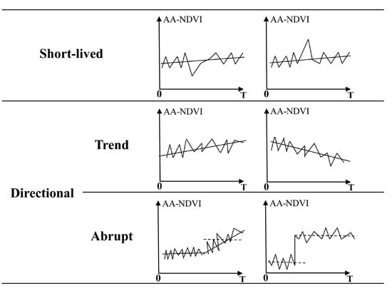
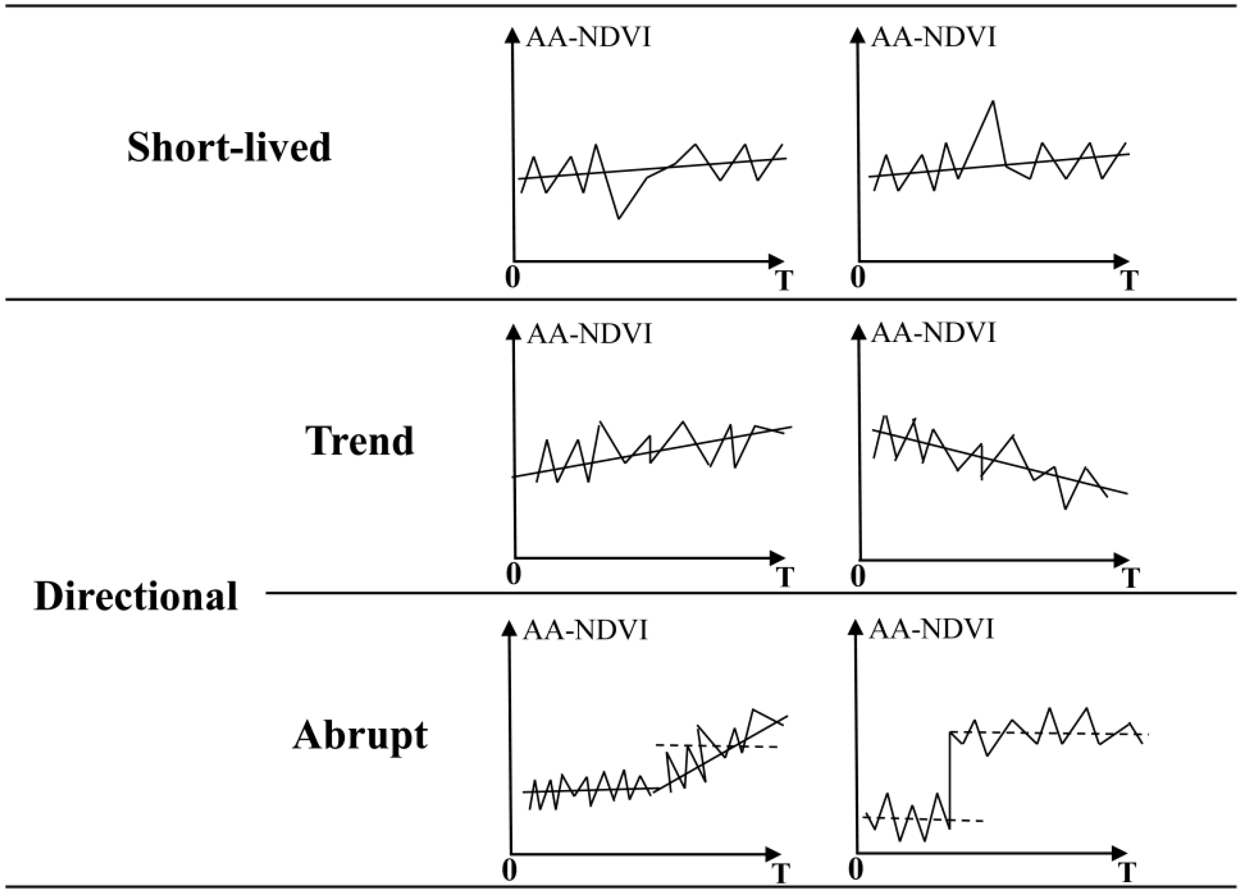
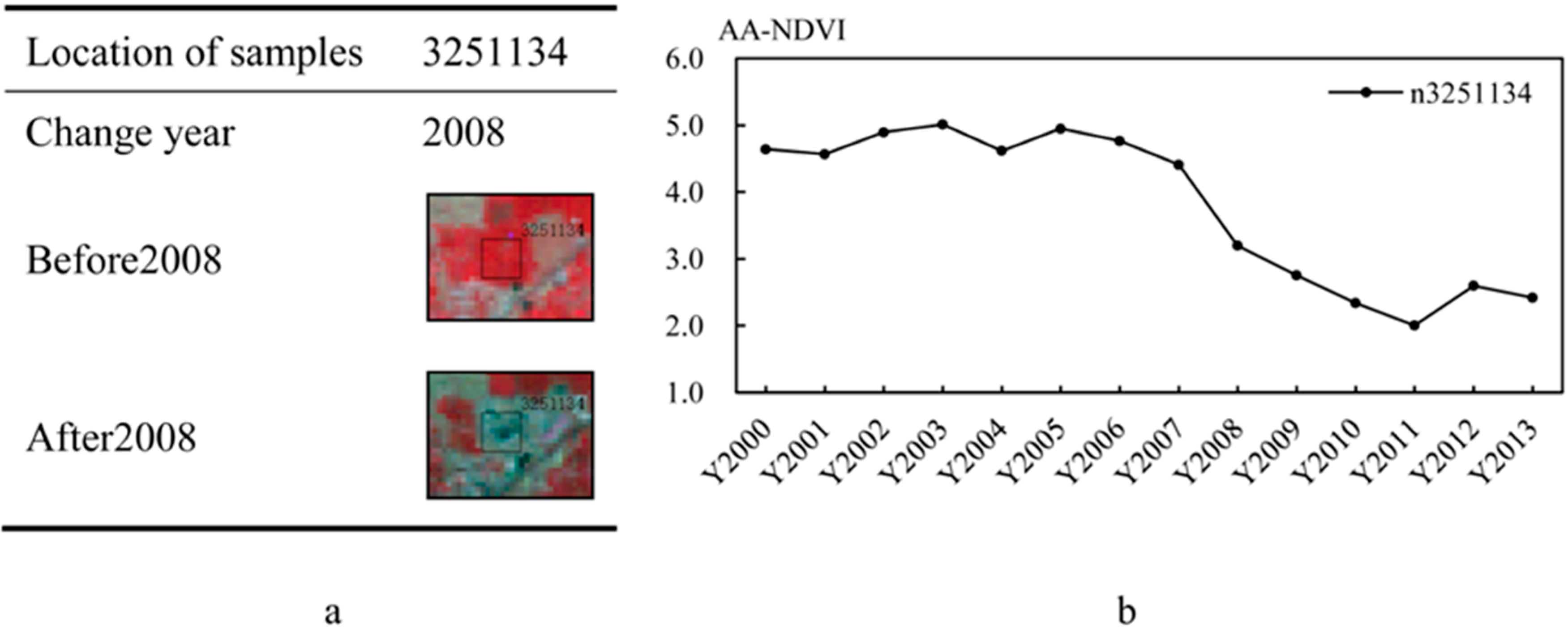
Framework of Change detection. Different land cover types present different AA-NDVI trajectories (Figure 2). Changes in land cover type or in the status of a land cover type can be illustrated by the change of the AA-NDVI trajectory. The general idea behind the method is to distinguish different types of land cover change based on changes of the AA-NDVI trajectories using different statistical methods.

The NDVIs of SCs can be considered outliers since their NDVIs were remarkably different from the normal value. Grubbs’ test [65] was used to determine these outliers in each of the AA-NDVI trajectories.

AA-NDVI trajectories of ACs cannot be detected just based on one method. The AA-NDVI trajectories before or after an AC point can be grouped into two classes: “no trend” and “with trend”. The “no trend” AA-NDVI trajectories generally belong to land cover types that have a stable status, e.g., natural vegetation such as grassland or forest in the climax stage of succession, or artificial land cover such as cropland (their pixel AA-NDVIs fluctuate with their averages). The “with trend” AA-NDVI trajectories generally belong to land cover types that reflect continuous positive or negative trends, e.g., forest or bush that is continually growing or being degraded. For an AA-NDVI trajectory whose subtrajectories before or after a specific point both indicated “no trend” (type NT abrupt land cover change), the BF test method, which can distinguish the mean jump in a time series [36,37], was used to determine whether an AC points existed.

For an AA-NDVI trajectory in which one or both subtrajectories before or after a specific point indicated “with trend” (type WT abrupt land cover change). Both the Tomé’s trend detection method [38,39] and the Chow test based on the difference of slopes of two segments [40] were used to determine whether an AC point existed. This method just tried to decrease the omission of land cover change which cannot be detection by BF test due to the similar mean of AA-NDVI between two segments of NDVIs in this kind of time series.

All of the trajectories that did not indicate ACs, whether they indicate a positive trend (vegetation greenness increase) or a negative trend (vegetation greenness decrease) will be determined. In this study, the SMK method was used to determine whether an AA-NDVI trajectory had a significant trend.

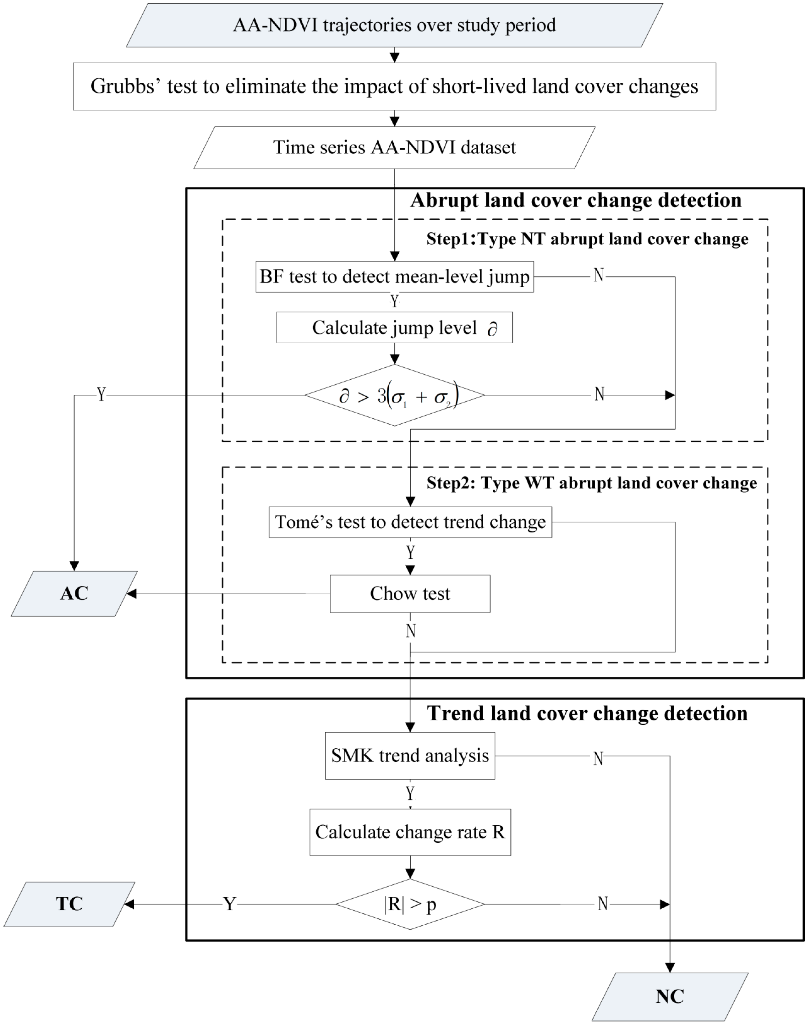
This study focused on directional land cover changes, and thus other statuses of land cover change were flagged as “no change” (NC). First, we eliminated the impact of SCs. Then, ACs were detected using the BF test or the combination of the Tomé’s method and Chow test. Finally, for all pixels indicating no AC in land cover, it was determined whether their trajectories indicated TCs (Figure 3).

2.3.2. Eliminating the Impact of Short-Lived Land Cover Changes

In this study, the Grubbs’ test [65] was used to determine SCs by considering them outliers in each AA-NDVI trajectory. The Grubbs’ test can be defined as follows:

$$G=\left|x_i-\overline{x}\right|/s$$

(1)

where $x_i$ is the i-th NDVI value in an AA-NDVI trajectory, and $\overline{x}$ and $s$ are the mean and standard deviation, respectively, of the AA-NDVIs. The hypothesis of no outliers is rejected if

$$G>\frac{N-1}{\sqrt{N}}\sqrt{\frac{{t^2}_{(\alpha /(2N),N-2)}}{N-2+{t^2}_{(\alpha /(2N),N-2)}}}$$

(2)

where t is the percent point function of the t distribution and N is the total number of time series. In this study, the significance level was 95% (p = 0.05).

The Grubbs’ test detects one outlier at a time. For multiple outliers, a detected outlier was deleted and the Grubbs’ test run again, following which the process was repeated until no further outliers were detected. The detected NDVIs as outliers were considered SCs and their NDVIs were replaced by the maximum (if the outlier was the maximum in the time series) or by the minimum NDVIs (if the outlier was the minimum in the time series), except for those NDVIs determined as outliers in the AA-NDVI trajectories.

2.3.3. Abrupt Land Cover Change Detection

(1)

Type NT Abrupt Land Cover Change Detection

The BF test provides a method with which to distinguish the mean jump points in a time series dataset with a small number of samples [36,37]. Compared with other methods, it does not require strict normality or heteroscedasticity in the original dataset [66]. The entire AA-NDVI trajectory can be treated as a time series: x = {$x_1$,$\dots$,$x_N$}. The AA-NDVI trajectory can be divided into m parts by (m – 1) abrupt points, following which the F statistics were calculated, as in Equations (3)–(7):

$$F=\frac{{{\displaystyle \sum }}_{i=1}^m{n}_i{\left(x_{i.}-x_{··}\right)}^2}{{{\displaystyle \sum }}_{i=1}^m\left(1-n_i/N\right)S_i^2}$$

(3)

where

$$N={\displaystyle \sum }_{i=1}^m{n}_i$$

(4)

$${\mathrm{x}}_{i.}={\displaystyle \sum }_{j=1}^{n_i}{x}_{ij}/n_i$$

(5)

$$x_{··}={\displaystyle \sum }_{i=1}^m{\displaystyle \sum }_{j=1}^{n_i}{x}_{ij}/N={\displaystyle \sum }_{i=1}^m{n}_i{x}_{i·}/N$$

(6)

$$S_i^2={\displaystyle \sum }_{j=1}^{n_i}{\left(x_{ij}-x_{i.}\right)}^2/\left(n_i-1\right)$$

(7)

The F statistics in the BF test are subject to the F-distribution with $\left(m-1,f\right)$ degrees of freedom (Equations (8) and (9)), where m is the number of parts divided by the abrupt points (m is 2 when there is only one jump point I), $n_i$ is the number of samples in the i-th part, N is the total number of samples (N was 14 in this study), $x_{i.}$ is the mean of the samples in the i-th part, $x_{\mathrm{..}}$ is the mean of the total samples, and $s_i^2$ is the variance of the samples in the i-th part.

$$f=\frac{1}{{{\displaystyle \sum }}_{i=1}^m{c}_i^2/\left(n_i-1\right)}$$

(8)

where

$$c_i=\left(1-n_i/N\right)S_i^2/\left[{\displaystyle \sum }_{i=1}^m\left(1-n_i/N\right)S_i^2\right]$$

(9)

F statistics was computed for all possible locations of abrupt points and the locations of abrupt points with the maximum F statistics ($F_{max}$) were selected as possible abrupt points.

In this study, the user needs to decide the minimum interval of two potential abrupt points (i.e., two years referenced as [32,34]) and thus the maximum number of abrupt points will be determined. Users will conduct the process based on Equations (1)–(9) starting with the case of one abrupt point and continuing up to the maximum number of abrupt points. The best segmentation was selected based on the abrupt points with the maximum $F_{max}$($F{\text{'}}_{max}$).

The hypothesis of no mean jump is rejected if

$$F{\text{'}}_{max}>F_{\mathsf{\alpha }}$$

(10)

where $F_{max}$ is the maximum F statistics among those at all locations of the abrupt point I (α = 0.05 in this study).

Because the variation of the AA-NDVIs was high and the difference of the means of some land cover types relatively low, the risk of type-II errors in the hypothesis test was high. A threshold of the difference of the NDVI means of two adjacent subparts was used to reduce this type of risk:

$$\partial =\left|\frac{{{\displaystyle \sum }}_1^{I-1}{x}_i}{n1}-\frac{{{\displaystyle \sum }}_{I+1}^N{x}_i}{n2}\right|$$

(11)

where $x_i$ is the NDVIs in each subpart, I is the location of the abrupt point, and $n1$ and $n2$ are the numbers of samples in two adjacent subparts. The threshold was developed referring to the principle of Zhu et al. [18], which was proposed for monitoring abrupt land cover changes:

$$\partial >3({\mathsf{\delta }}_1+{\mathsf{\delta }}_2)$$

(12)

where ${\mathsf{\delta }}_1$ and ${\mathsf{\delta }}_2$ represent the standard deviations of two adjacent subparts.

(2)

Type WT Abrupt Land Cover Change Detection

Tomé’s method is a piecewise fitting method that can determine the detailed trend change within a time series [38,39]. Because the number of abrupt points in a time series is set arbitrarily using Tomé’s method, we used the Chow test [40] to determine whether the potential abrupt points were also abrupt points based on Tomé’s method, such that abrupt land cover changes could be detected automatically.

Suppose there is one breakpoint in a time series y = {$y_1$,$\dots$,$y_N$} and the location of the abrupt point may be $t_{bp\left(2\right)}$($t_{bp\left(2\right)}=3, \dots , N-2$). The entire time series can be divided into two segments that could be expressed by two linear equations (Equations (13) and (14)):

$${\mathit{y}}_{\mathit{i}}\mathbf{=}{\mathit{a}}_{\mathbf{1}}{\mathit{t}}_{\mathit{i}}\mathbf{+}{\mathit{c}}_{\mathbf{1}} i=\mathit{1},..., {\mathit{t}}_{\mathit{b}\mathit{p}\left(\mathbf{2}\right)}$$

(13)

$${\mathit{y}}_{\mathit{i}}\mathbf{=}{\mathit{a}}_{\mathbf{2}}{\mathit{t}}_{\mathit{i}}\mathbf{+}{\mathit{c}}_{\mathbf{2}} i= {\mathit{t}}_{\mathit{b}\mathit{p}\left(\mathbf{2}\right)}+\mathit{1},...,N$$

(14)

where N is the total number within the entire time series, and $a_1$,$a_2$,$c_1$, and$c_2$ are parameters. Because the two segments are continuous, we can obtain Equation (15):

$$c_2=c_1+\left(a_1-a_2\right)t_{bp\left(2\right)}$$

(15)

Therefore, there are three unknown solutions for this series of linear equations. Suppose $s$ is the vector solution, s = {$a_1$,$a_2$,$c_1$}, and A is a rectangular matrix ($2\times 3$) with its first line equal to {$t_i,0,1$} and its second line equal to {$t_{bp\left(2\right)}, t_i-t_{bp\left(2\right)},1$}. Then, the solutions can be obtained by solving Equation (16):

$$T_{min}=min||y-As||$$

(16)

Thus, we can determine the possible locations of the abrupt points. The same strategy can also be used when there is more than one abrupt point. When the user decides the minimum interval of two potential abrupt points and thus the maximum number of abrupt points will be also determined. The most possible number of abrupt points can be determined based on minimum $T_{min}$with different numbers of abrupt points. Tomé’s method suggests that users start with the case of one abrupt point and continue up to the presupposed maximum number of abrupt points, such that all of the abrupt points could be determined automatically. In this study, the Chow test, which was used to determine whether the two segments separated by abrupt points were significantly different, was calculated as shown in Equation (17):

$$F_{chow}=\frac{[RS{S}_c-\left(RS{S}_1+RS{S}_2\right)]/k}{(RS{S}_1+RS{S}_2)/\left(N-2k\right)}$$

(17)

where $RS{S}_c$ is the sum of the squared residuals over the entire time series, $RS{S}_1$ and $RS{S}_2$ are the sums of the squared residuals of two segments before and after the potential abrupt point, respectively, N is the total number of dates in the two segments, k is the cost in degrees of freedom, and (N − 2k) is the remaining degrees of freedom.

$F_{chow}$ subjects to the F-distribution with (k, (N − 2k)) degrees of freedom. The hypothesis of “no trend” difference before and after the abrupt point is rejected if

$$F_{chow}>F_{\mathsf{\alpha }}$$

(18)

We concluded there was significant difference in the AA-NDVI trends before and after the abrupt point and considered it a real abrupt point (α = 0.05 in this study).

2.3.4. Trend Land Cover Change Detection

In this study, the SMK method was used to determine whether an AA-NDVI trajectory indicated significant trend. SMK is a non-parametric method that is robust against non-normality of a dataset [67]. The trend slope can be defined as in Equation (19):

$$\mathsf{\beta }=Median\left(\frac{X_j-X_i}{j-i}\right), \forall j>i$$

(19)

where $X_j$ and $X_i$ are NDVIs in a time series of AA-NDVIs and $\mathsf{\beta }$ is the trend slope of the time series. The condition $\mathsf{\beta }$ > 0 means a positive trend of vegetation growth during the study period, while $\mathsf{\beta }$ < 0 means a negative trend. The significance of the slope can be determined using the Mann-Kendall test as in Equations (20)–(24):

$$U_{MK}=\frac{\mathsf{\tau }}{{\left[Var\left(\mathsf{\tau }\right)\right]}^{1/2}}$$

(20)

where

$$\mathsf{\tau }={\displaystyle \sum }_{i=1}^{n-1}{\displaystyle \sum }_{j=i+1}^{n}sgn\left(X_j-X_i\right)$$

(21)

$$sgn\left(\mathsf{\theta }\right)=\{\begin{array}{c}1 if \mathsf{\theta }>0\\ 0 if \mathsf{\theta }=0\\ -1 if \mathsf{\theta }<0\end{array}$$

(22)

$$Var\left(\mathsf{\tau }\right)=\frac{n\left(n-1\right)\left(2n+5\right)}{18}$$

(23)

where $X_j$ and $X_i$ are NDVIs in an AA-NDVI series and $n$ is the number of dates. The hypothesis of no AA-NDVI trend is rejected if

$$\left|U_{MK}\right|>U_{\raisebox{1ex}{$\mathsf{\alpha }$}\!\left/ \!\raisebox{-1ex}{$2$}\right.}$$

(24)

Finally, the NDVI change rate over the study period, which directly expresses the magnitude of trend change, can be determined using Equations (25) and (26):

$$S_{\mathsf{\Delta }NDVI}=\left|\frac{\left(\mathsf{\beta }\times t_{\mathrm{n}}+a\right)-\left(\mathsf{\beta }\times t_1+a\right)}{\mathsf{\beta }\times t_1+a}\right|\times 100$$

(25)

$$a=\overline{X}-\mathsf{\beta }\times \overline{t}$$

(26)

where $S_{\mathsf{\Delta }NDVI}$ is the NDVI change rate (percentage of AA-NDVI increase over the study period), $\overline{X}$ is the mean of the time series of NDVIs, $\overline{t}$ is the mean value of the dates, and $t_1$ and $t_n$ are the start and end years of the time series, respectively. The area of TC can be acquired using Equation (27):

$$\left|S_{\mathsf{\Delta }NDVI}\right|>p$$

(27)

where $p$ is the change rate threshold, which was set as 10 in this study.

2.4. Technique Validation

2.4.1. Accuracies of Abrupt Land Cover Changes

In this study, land cover changes were reclassified into two classes: abrupt changes and no abrupt changes. Abrupt changes included both NT and WT, as discussed in Section 2.3.1; no abrupt changes included both TC and NC.

The confusion matrix method was used to assess the accuracies of the abrupt change land cover map. Indices such as the overall accuracy, kappa index, user’s accuracy, producer’s accuracy, commission error, and omission error were used. A stratified random sampling scheme was used to obtain 200 samples for this assessment.

Validation of change detection results is notoriously difficult because ground truth data of historical land cover changes are usually unavailable [9,18,32]. In this study, we mainly used remote sensing images with high spatial resolutions (30 m or higher) to validate the abrupt changes in land cover because of their relatively fine and accurate representation [9,18]. We obtained the validation data through visual interpretation of the remotely sensed images. The profiles of the AA-NDVI trajectories were also used to help in understanding the land cover changes (Figure 4). Field visits and interviews were also conducted in August 2015, such that a clear relationship between the present and historical images could be confirmed for all sample points.

If abrupt land cover change occurred in a MODIS pixel, the land cover change in the area of this pixel had to meet two criteria. First, the area of the land cover type change had to be >60% when the land covers in the major part of this pixel had changed and second, the land cover could not revert throughout the duration of the study period following the appearance of the abrupt land cover change. To determine whether the land cover changes met the first criterion, we selected the LTS images before or after an abrupt point. Then, the land covers were classified in the area of the sample MODIS pixels based on visual interpretation of the two LTS images. Finally, the classified land cover map was overlaid and the percentage statistics of the areas in which the land cover types had changed were calculated. To determine whether the land cover changes met the second criterion, the stability of the AA-NDVI trajectory after the abrupt point was assessed through visual interpretation of its profiles of the AA-NDVIs (Figure 4).

To determine whether no abrupt land cover changes occurred in a sample MODIS pixel, at least two stages of land cover changes were interpreted for a validation sample based on three images from 2000, 2005, or 2010. If the land cover changes in a pixel could not meet both criteria discussed above, the land cover changes were considered as no abrupt change.

2.4.2. Accuracies of Trend Land Cover Changes

Because the validation of the trend change based on ground truth data was unrealizable until now [32], we can only give some benchmark for the land cover change detection. In this study, two methods were used: (1) consistency evaluation of NDVI change trends over the study period between LTS and MODIS datasets; and (2) consistency evaluation between millet yield per unit and average NDVIs of cropland for each banner.

For the consistency evaluation of the NDVI change trends between LTS and MODIS datasets, 100 MODIS pixels were selected at random from areas with trend land cover change. In order to make a quantitative comparison between different Landsat images, relative radiometric correction based on Radio-metric Control Set (RCS) [10], was used to correct the surface reflectance to guarantee spatio-temporal consistency in reflectance values [68]. The averages of the NDVIs in the area of a MODIS sample pixel were computed based on a summer LTS image for at least three years, and their trends were also determined. At the same time, the trend of the MODIS NDVI for the same pixel was also determined. If the observed trend (positive or negative) in the sample pixel was the same, we defined its land change trend as consistent. The percentage of samples indicating the consistency was computed using Equation (28):

$$PSC=\frac{Nc}{Ns}\times 100\%$$

(28)

where PSC is the percentage of samples indicating the consistency, Ns is the total number of selected samples, and Nc is the number of samples that indicated a consistent change trend.

As discussed in Section 3.1, because 47.9% of trend land cover changes during the study period were related to cropland, we also validated the land cover trend changes for cropland. Because a high millet yield within an area indicates high crop biomass, it has a high NDVI value [69]; thus, the consistency evaluation between millet yield per unit and average NDVIs of cropland for the entire study area and each banner was also conducted. Here, we used a simple linear regression to test the strength of the linear association between millet yield per unit (independent variable) and average NDVIs of cropland (dependent variable) over the study period. It was a limitation of this study that we could not obtain suitable grassland productivity change data to validate the NDVI trend in grassland.

3. Results

3.1. Land Cover Changes

From 2000 to 2013, land cover in the study area indicated remarkable changes (

Table 2. Land cover changes in the study area.

	Abrupt Change	Trend Change	No Change
Area (km2)	2176.3	44,574.9	83,638.7
Percentage (%)	1.7%	34.2	64.1

, Figure 5b). About 35.9% of the entire study area (46,751.2 km²) showed directional land cover changes, of which 34.2% (44,574.9 km²) indicated TCs and 1.7% (2176.3 km²) indicated ACs.

The NDVIs clearly indicated a positive trend in the trend land cover changes. The area in which the NDVIs indicated a positive trend was 4246.2 km² (95.3% of the total area of trend land cover changes). The NDVIs indicated a negative trend for only 2112.7 km² (4.7% of the total area of trend land cover changes). The area in which the NDVI increased by >20% during the study period was 33,230.4 km² (74.5% of the total area of trend land cover changes). The area in which the NDVI decreased by >20% during the study period was 1184.3 km² (2.5% of the total area of trend land cover changes).

The trend land cover changes occurred mainly in cropland and grassland areas (

Table 3. Area of trend land cover changes with different change rates related to land cover types.

Change Rate		Cropland	Grassland	Woodland	Wetland	Built-Up Area	Unused Land	Total
>40	km2	4496.6	3044.3	1246.7	181.6	148.6	539.8	9657.6
	%	10.1	6.8	2.8	0.4	0.3	1.2	21.7
20–40	km2	11,959.6	8139.9	1691.7	214.5	585.5	981.6	23,572.8
	%	26.8	18.3	3.8	0.5	1.3	2.2	2.9
10–20	km2	4600.4	2936.5	596.8	74.3	384.5	639.3	9231.8
	%	10.3	6.6	1.3	0.2	0.9	1.4	20.7
−10–−20	km2	163.1	433.4	117.0	20.1	40.6	154.2	928.4
	%	0.4	1.0	0.3	0.0	0.1	0.3	2.1
−20–−40	km2	96.2	530.6	62.0	52.0	51.9	219.2	1011.9
	%	0.2	1.2	0.1	0.1	0.1	0.5	2.3
<−40	km2	21.0	56.0	2.8	46.5	21.2	24.9	172.4
	%	0.0	0.1	0.0	0.1	0.0	0.1	0.3
Total	km2	21,336.9	15,140.7	3717.1	588.9	1232.3	2559.0	44,574.9
	%	47.9	34.0	8.3	1.3	2.8	5.7	100

, Figure 5). The changed area related to these two land cover types was 36,477.6 km² (81.9% of the total area of trend land cover changes). The area in which trend land cover change occurred in cropland was 21,336.9 km² (47.9% of the total area of trend land cover changes). The area in which trend land cover change occurred in grassland was 15,140.7 km² (34.0% of the total area of trend land cover changes).

The NDVI indicated the trend in cropland more clearly than in grassland (Table 3). The areas of cropland and grassland in 2010 were 49,149.9 and 67,562.2 km², respectively. However, their areas of trend change were 21,336.9 and 15,140.7 km², accounting for 43.4% and 22.4%, respectively, of their total areas; i.e., the percentage of cropland indicating trend land cover change was nearly twice that of grassland.

Abrupt land cover changes occurred mainly in the middle part of the semi-pastoral banners in the study area (Figure 6a). In Kailu County, Horqin District, and Naiman Banner, the percentages of abrupt land cover change area to total land cover change area were from 11.1% to 22.6%, much higher than for the entire study area (1.7%) (Figure 7a). These areas are located mainly in the West Liao River Plain, which has the highest population density within the study area. The changed areas were concentrated primarily around residential communities. Other abrupt land cover changes occurred alongside major transportation networks or around the towns of counties. Thus, it appears that abrupt land cover changes are largely related to human activities.

Trend land cover changes occurred mainly in the southern and middle parts of the study area (Figure 6b), although some changes occurred in the northeast. All of these areas are also located in semi-pastoral banners. In Hure Banner, Aohan Banner, Naiman Banner, and Kailu County, the percentages of trend land cover change area to total trend land cover change area were 14.1%, 12.1%, 11.3%, and 9.1%, respectively (Figure 7). In these areas, the major land cover type is cropland (Figure 5). Thus, it appears that the trend land cover changes were also largely related to human activities such as farmland fertilization, irrigation and pest control.

3.2. Accuracy Assessment

3.2.1. Accuracies of Abrupt Land Cover Changes

The accuracies of the abrupt land cover changes were indicated as high. The overall accuracy of the abrupt land cover changes was 87.0%, and the kappa index was about 0.74 (

Table 4. Error matrix for detecting abrupt land cover changes.

		Reference
		Abrupt Changes	No Abrupt Changes	Total	User’s Accuracy	Commission Error
Classified	Abrupt changes	80	20	100	80.0%	20.0%
	No abrupt changes	6	94	100	94.0%	6.0%
	Total	86	114	200
	Producer’s accuracy	93.0%	82.5%	Overall accuracy = 87.0%
	Omission error	7.0%	17.5%	Kappa index = 0.74

). The user’s accuracy was 80.0%, while the producer’s accuracy was about 93.0%. The user’s accuracy of no abrupt changes was 82.5%, while the producer’s accuracy was about 94.0%.

The accuracies of abrupt land cover changes included more commission errors. The commission error of abrupt changes was as high as 20.0%, while its omission error was about 7.0%. The accuracies of no abrupt land cover changes included more omission errors. The omission error of no abrupt changes was 17.5%, while its commission error was about 6.0%.

3.2.2. Accuracies of Trend Land Cover Changes

The trends evaluation indicated high consistency between the NDVI change trends from the LTS and MODIS datasets. Of the 100 samples, all indicated the same trend (positive or negative) of vegetation growth in the sample areas in the MODIS dataset and the LTS images, and the percentage of samples indicating consistency was 100%.

In cropland areas, the trends of millet yield per unit and the average NDVIs also indicated high consistency. In the entire study area, we found that the change trajectories of millet yield per unit and the average NDVIs of cropland during the study period were highly consistent (Figure 8), and that the average NDVIs of cropland could be predicted based on a linear regression with a coefficient of determination of 0.94 (p < 0.01) (

Table 5. Results of simple linear regression.

Statistical Area	Equation of Linear Regression	R2	p
Tuquan County	y = 0.31x + 3.21	0.66	p < 0.01
Horqin Right Middle Banner *	y = 0.26x + 3.59	0.55	p < 0.01
Jarud Banner *	y = 0.46x + 2.96	0.46	p < 0.01
Ar Horqin Banner *	y = 0.47x + 3.27	0.79	p < 0.01
Horqin Left Middle Banner *	y = 0.16x + 3.54	0.79	p < 0.01
Bairin Left Banner *	y = 0.43x + 3.58	0.73	p < 0.01
Bairin Right Banner *	y = 0.16x + 3.91	0.13	p = 0.20
Kailu County	y = 0.36x + 2.25	0.86	p < 0.01
Horqin District	y = 0.70x + 0.49	0.55	p < 0.01
Horqin Left Back Banner *	y = 0.47x + 2.73	0.69	p < 0.01
Naiman Banner	y = 0.35x + 2.93	0.69	p < 0.01
Ongniud Banner *	y = 0.40x + 2.57	0.70	p < 0.01
Hure Banner	y = 0.25x + 3.21	0.78	p < 0.01
Aohan Banner	y = 0.43x + 2.88	0.72	p < 0.01
The whole study area	y = 0.42x + 2.72	0.94	p < 0.01

* Banners (counties or cities) of pastoral area in Figure 1.

). In all of the banners or counties, except for Bairin Right Banner, there were strong linear associations between millet yield per unit and average NDVIs of cropland throughout the study period. Average NDVIs of cropland could also be predicted based on a linear regression with a coefficient of determination from 0.46 to 0.86 (p < 0.01).

4. Discussion

4.1. Improvement of MTHD Method

We compared the detection results based on BFAST method and MTHD method, taking the typical sample (No. 3251134) mentioned in Figure 4. Validation results indicated a land cover conversion from cropland to built-up area in 2008 (Figure 4a). In MTHD, we used AA-NDVIs trajectory as input. BFAST took the whole time series (including intra-annual variations) as inputs. Result of MTHD showed that there was an abrupt change in 2008 and the same to the validation (Figure 4b).

Results of BFAST indicated that there are two abrupt points in trend component (Tt), the first abrupt appeared during 2005~2006 and the second abrupt appeared during 2010~2011 (Figure 9). These two abrupt points were not related with specific land cover change closely because land cover conversion happened only in 2008 as MTHD did.

In addition, the land cover changes detected based on the Grubbs’ test could be considered short-lived, whereas those detected based on the BF test or the combination of the Tomé’s method and Chow test could be considered abrupt, indicating a change of land cover type. The changes detected using the SMK method were trend changes, indicating significant trend change without change of land cover type. This indicated that the land cover changes detected using the MTHD method could be related closely to specific ecosystem changes (i.e., land cover conversion and land cover modification). Although the BFAST and DBEST methods can also detect both abrupt and trend changes, it is very difficult to relate the detected changes to specific ecosystem changes (i.e., land cover conversion or land cover modification).

The BFAST and DBEST methods define abrupt change points based on an optimal overall fitting of an entire series instead of the evaluated differences between two subparts separated by each potential change point. These methods use a minimized Bayesian Information Criterion, which reflects the balance between the fitting residuals and model complexity, to determine the locations and numbers of abrupt change points. A point with a relatively large NDVI residual within a trajectory (the lowest NDVI in 2011) influenced the overall fitting performance of a series, making it more likely to be chosen as an abrupt change point where there were no “real” abrupt land cover changes. On the contrary, the lowest NDVI cannot have an effect on the detection results using MTHD. Therefore, The BFAST and DBEST methods could result in false detections easier in areas where the vegetation status usually changes with frequent and strong interannual fluctuations, such as arid or semi-arid areas. These two methods are more suitable for land cover change detection in humid areas where vegetation status is more stable with less intra-annual and inter-annual variations.

The MTHD method defines an abrupt point by comparing the differences of the means or slopes of AA-NDVI trajectories before and after a specific point. The means or slopes during a period can indicate the average status of vegetation growth. Thus, their changes are more reliable in representing any change of land cover type in comparison with the focus on the AA-NDVIs of an individual point. Furthermore, detecting abrupt land cover changes using the MTHD method is more robust and it can reduce the risk of false changes in AA-NDVI trajectories with frequent and strong interannual fluctuations.

4.2. Errors of Abrupt Land Cover Changes

As discussed in Section 3.2.1, the errors of abrupt land cover changes were mainly commission errors (20%). We considered all of the no-abrupt-change samples that were misclassified as abrupt points. It was established that these errors were caused by limited land cover changes within a MODIS pixel and changes of crop species within cropland areas. Limited land cover changes indicated that part of the land cover type had changed (but <60% within a sample pixel). The changed land covers could clearly affect the AA-NDVI trajectories, and thus they could be detected by the MTHD method. This type of misclassification of sample pixels occurred in 11 of 20 samples (55%) (

Table 6. Commission error sources and graphical representation of changes.

Error	Error Sources	Samples		Graphical Representation (from → to)	Descriptions for Graphical Representation
		Amount	Percentage
Commission	Limited land cover changes	11	55.0%		A mixed pixel with type A and B turned to a pixel with type A, less than 60% of land cover type changes in a pixel happened.
	Changes of crop species in cropland	9	45.0%		Crop changed from corn to vegetable in a pixel.
Omission	Counteracting spectral effects	4	66.7%		A pixel with type B turn to a mixed pixel with type B, type A with high NDVIs and C with low NDVIs.
	Swap changes	2	33.3%		A mixed pixel with type A and B. While A and B were swap more than 60% to each other within the pixel.

). In some cropland areas, the planted crops varied over the duration of the study period. Different crop species clearly indicated different AA-NDVI trajectories, and thus some sample pixels were also misclassified as ACs. This type of misclassification of sample pixels occurred in nine of 20 samples (45%) (Table 6).

Omission errors (7%) were largely caused by land cover changes indicating counteracting spectral effects and land cover swap changes. In some mixed MODIS pixels, different land cover types indicated quite different NDVIs. The NDVI of the changed MODIS pixel might not change clearly because of the counteracting effect of high and low NDVIs of changed land cover types within the same MODIS pixel. Thus, this type of sample pixel could be misclassified as having no abrupt change. This type of misclassification of sample pixels occurred in four of six samples (66.7%) (Table 6). Land cover swap change refers to a loss in the amount of a land cover type at a specific location that is accompanied by the same amount of gain of this type in another location [70]. This happens frequently in some arid or semiarid zones in China because of the high variation in precipitation and irrational human activities [71]. In a 250-m MODIS pixel, although the percentages of different land cover type areas are the same and the spectral features are similar, the actual land covers could change by >60% of the entire pixel because of land cover swap changes. Thus, this type of sample pixel could be misclassified as having no abrupt changes. This type of misclassification of sample pixels occurred in two of six samples (33.3%) (Table 6).

4.3. Limitations and Further Research

4.3.1. Limitations in Detecting Abrupt Land Cover Changes

To detect both abrupt and trend land cover changes within the same framework, the MTHD method detects these changes based on a time series NDVI dataset, similar to the BFAST and DBEST methods. However, these methods cannot detect abrupt land cover change within a few points of the beginning or end of the study period. Thus, the abrupt land cover change detection in MTHD cannot be used in real-time monitoring of land cover change on a yearly scale. In addition, although the detected land cover changes using the MTHD method could be related to ecosystem changes, this method can only determine change or no change of land cover changes. If it is required to obtain specific “from–to” classes of abrupt land cover change and to detect real-time changes on a yearly scale, the MTHD method will have to be improved.

4.3.2. Limitation of Data Sources

To mitigate the effects of frequent and strong interannual variations, the MTHD method uses AA-NDVI trajectories as inputs. Thus, the temporal resolution of these inputs must be at least one cloud-free mosaic image per month during the growing season. However, it was difficult to obtain such input data from commonly used medium-spatial-resolution remote sensing data such as TM/ETM+, Système Probatoire d’Observation de la Terre, Advanced Spaceborne Thermal Emission and Reflection Radiometer, or China-Brazil Earth Resources Satellite (CBERS) because of the impact of clouds. Therefore, in this study, we chose to use MODIS NDVI as inputs.

Because of the coarse spatial resolution of MODIS data, the mixed pixels of the MODIS data decreased the accuracies of the abrupt land cover changes. As discussed in Section 4.2, 11 of 20 samples (55.0%) were related to mixed pixels of MODIS data with regard to the commission error, and all six samples were related to mixed pixels of MODIS data with regard to the omission error. Overall, 17 of 26 samples (65.4%) were related to mixed pixels with regard to the misclassification of abrupt land cover changes.

The limitations regarding data sources could be resolved very soon. Sensors capable of both high temporal and fine spatial resolutions have already been launched or will soon be launched. China’s GF-1 satellite, launched in 2013, is equipped with multispectral scanners with 16-m resolution and most areas will be revisited every two days. The Sentinel-2 A/B Multispectral Instrument, manufactured by the European Space Agency, will be equipped with four, six, and three bands with 10-, 20-, and 60-m spatial resolutions, respectively. With two satellites, most areas will be revisited every five days under the same viewing conditions, and the revisit frequency will be increased with different viewing conditions (Sentinel-2 A was launched in 2015 and Sentinel-2 B is scheduled for launch in 2016) [72].

4.3.3. Other Uncertainties

In data preprocessing, the choices of reconstruction methods and the determination of high-quality pixels are two main uncertainty sources. In this study, MTHD used SG filter to decrease noises, and defined the high-quality pixel by referencing the pixel reliability in layer 12 of MODIS 13Q1product. Further study could apply more suitable reconstruction method, and utilize Vegetation Index usefulness information in layer 3 of MODIS 13Q1 product to determine high quality pixels accurately from the “marginal pixels” with a reliability rank of “1”.

In order to make MTHD be general and conducted automatically without the support of land cover maps, and to decrease the risk of false change detection caused by the high inter-seasonal variation of vegetation in arid and semi-arid zones, we chose the growing season (from 145 day to 273 day) as “seasonal window”. However, the NDVIs of different land cover types indicated different intra-annual patterns. It may be helpful to detect land cover changes based on different seasonal window with different land cover types. Therefore, further study should improve how to automatically extract and apply the seasonal features of NDVI series of each pixel in land cover change detection.

Validation of change detection results is notoriously difficult because ground truth data of historical land cover changes are mostly unavailable. In this study, we took Landsat time series image dataset as the main source of validation data and the collection of validation data relied on visual interpretation. Thus, the validation data were not real “ground truth” ones and the accuracy assessment may contain some uncertainty. Therefore, it is very important to establish database of ground truth data for land cover detection over a long period.

5. Conclusions

This paper proposed a multi-target hierarchical detection (MTHD) method to detect multiple directional land cover changes automatically. The MTHD technique used a hierarchical strategy to detect directional changes (including both abrupt changes (ACs) and trend changes (TCs)) successively. Compared with other multi-target change detection methods, the land cover changes detected by the MTHD method could be related more closely to specific ecosystem changes. Furthermore, the MTHD method could reduce the risk of false changes in AA-NDVI trajectories with frequent and strong interannual fluctuations. We applied the MTHD method to the Horqin Sandy Land using MODIS13Q1 (Moderate Resolution Imaging Spectroradiometer) NDVI time series datasets. The results demonstrated that both abrupt and trend land cover changes could be detected accurately and automatically.

Although the MTHD method can detect both abrupt and trend land cover changes automatically over a large area, it cannot detect abrupt land cover change within a few years of the beginning or end of a study period, similar to other methods. Further study will be required to address this issue. Furthermore, because we used MODIS data with coarse spatial resolution as the only input, the accuracies of the abrupt land cover change were reduced because of the effect of mixed pixels. This limitation could be resolved in the future using data sources with higher temporal and finer spatial resolutions, such as will be provided by the multispectral scanners of the GF-1 and Sentinel-2 satellites. Intra-annual patterns of the NDVIs of different land cover types can be helpful to improve the accuracy of land cover change detection. Therefore, further study should also improve how to automatically extract and apply the seasonal features of NDVI series of each pixel in land cover change detection.

References

1. Lu, D.; Mausel, P.; Brondizio, E.; Moran, E. Change detection techniques. Int. J. Remote Sens. 2004, 25, 2365–2401. [Google Scholar] [CrossRef]
2. Hobbs, R.J. Remote sensing of spatial and temporal dynamics of vegetation. In Remote Sensing of Biosphere Functioning, 1st ed.; Hobbs, R.J., Mooney, H.A., Eds.; Springer-Verlag: New York, NY, USA, 1990; pp. 203–219. [Google Scholar]
3. Scheffer, M.; Carpenter, S.; Foley, J.A.; Folke, C.; Walker, B. Catastrophic shifts in ecosystems. Nature 2001, 413, 591–596. [Google Scholar] [CrossRef] [PubMed]
4. Kennedy, R.E.; Andrefouet, S.; Cohen, W.B.; Gomez, C.; Griffiths, P.; Hais, M.; Healey, S.P.; Helmer, E.H.; Hostert, P.; Lyons, M.B.; et al. Bringing an ecological view of change to Landsat-based remote sensing. Front. Ecol. Environ. 2014, 12, 339–346. [Google Scholar] [CrossRef] [Green Version]
5. Lambin, E.F.; Geist, H.J. Land-Use and Land-Cover Change: Local Processes and Global Impacts; Springer: Berlin, Germany, 2006; pp. 33–39. [Google Scholar]
6. Lu, D.; Li, G.; Moran, E. Current situation and needs of change detection techniques. Int. J. Image Data Fusion 2014, 5, 13–38. [Google Scholar] [CrossRef]
7. Verbesselt, J.; Zeileis, A.; Herold, M. Near real-time disturbance detection using satellite image time series. Remote Sens. Environ. 2012, 123, 98–108. [Google Scholar] [CrossRef]
8. Jin, S.; Sader, S.A. MODIS time-series imagery for forest disturbance detection and quantification of patch size effects. Remote Sens. Environ. 2005, 99, 462–470. [Google Scholar] [CrossRef]
9. De Jong, R.; Verbesselt, J.; Zeileis, A.; Schaepman, M.E. Shifts in global vegetation activity trends. Remote Sens. 2013, 5, 1117–1133. [Google Scholar] [CrossRef] [Green Version]
10. Zhou, Q.M.; Li, B.L.; Chen, Y.M. Remote sensing change detection and process analysis of long-term land use change and human impacts. Ambio 2011, 40, 807–818. [Google Scholar] [CrossRef] [PubMed]
11. Dubinin, M.; Luschekina, A.; Radeloff, V.C. Climate, livestock, and vegetation: What drives fire increase in the arid ecosystems of southern Russia? Ecosystems 2011, 14, 547–562. [Google Scholar] [CrossRef]
12. De Jong, R.; de Bruin, S.; de Wit, A.; Schaepman, M.E.; Dent, D.L. Analysis of monotonic greening and browning trends from global NDVI time-series. Remote Sens. Environ. 2011, 115, 692–702. [Google Scholar] [CrossRef] [Green Version]
13. Forkel, M.; Carvalhais, N.; Verbesselt, J.; Mahecha, M.D.; Neigh, C.S.; Reichstein, M. Trend change detection in NDVI time series: Effects of inter-annual variability and methodology. Remote Sens. 2013, 5, 2113–2144. [Google Scholar] [CrossRef]
14. Eckert, S.; Hüsler, F.; Liniger, H.; Hodel, E. Trend analysis of MODIS NDVI time series for detecting land degradation and regeneration in Mongolia. J. Arid Environ. 2015, 113, 16–28. [Google Scholar] [CrossRef]
15. Coppin, P.; Jonckheere, I.; Nackaerts, K.; Muys, B.; Lambin, E. Review Article Digital change detection methods in ecosystem monitoring: A review. Int. J. Remote Sens. 2004, 25, 1565–1596. [Google Scholar] [CrossRef]
16. Singh, A. Review article digital change detection techniques using remotely-sensed data. Int. J. Remote Sens. 1989, 10, 989–1003. [Google Scholar] [CrossRef]
17. Kennedy, R.E.; Cohen, W.B.; Schroeder, T.A. Trajectory-based change detection for automated characterization of forest disturbance dynamics. Remote Sens. Environ. 2007, 110, 370–386. [Google Scholar] [CrossRef]
18. Zhu, Z.; Woodcock, C.E. Continuous change detection and classification of land cover using all available Landsat data. Remote Sens. Environ. 2014, 144, 152–171. [Google Scholar] [CrossRef]
19. Cohen, W.B.; Yang, Z.; Kennedy, R. Detecting trends in forest disturbance and recovery using yearly Landsat time series: 2. TimeSync—Tools for calibration and validation. Remote Sens. Environ. 2010, 114, 2911–2924. [Google Scholar] [CrossRef]
20. Kennedy, R.E.; Yang, Z.; Cohen, W.B. Detecting trends in forest disturbance and recovery using yearly Landsat time series: 1. LandTrendr—Temporal segmentation algorithms. Remote Sens. Environ. 2010, 114, 2897–2910. [Google Scholar] [CrossRef]
21. Piao, S.L.; Wang, X.; Ciais, P.; Zhu, B.; Wang, T.; Liu, J. Changes in satellite-derived vegetation growth trend in temperate and boreal Eurasia from 1982 to 2006. Glob. Chang. Biol. 2011, 17, 3228–3239. [Google Scholar] [CrossRef]
22. Adosi, J.J. Seasonal variation of carbon dioxide, rainfall, NDVI and it’s association to land degradation in Tanzania. In Climate and Land Degradation; Sivakumar, M.V., Ndiang’Ui, N., Eds.; Springer: Berlin/Heidelberg, Germany, 2007; pp. 373–389. [Google Scholar]
23. Li, Z.; Huffman, T.; McConkey, B.; Townley-Smith, L. Monitoring and modeling spatial and temporal patterns of grassland dynamics using time-series MODIS NDVI with climate and stocking data. Remote Sens. Environ. 2013, 138, 232–244. [Google Scholar] [CrossRef]
24. Geerken, R.A. An algorithm to classify and monitor seasonal variations in vegetation phenologies and their inter-annual change. ISPRS J. Photogramm. 2009, 64, 422–431. [Google Scholar] [CrossRef]
25. Olsson, L.; Eklundh, L.; Ardö, J. A recent greening of the Sahel-trends, patterns and potential causes. J. Arid Environ. 2005, 63, 556–566. [Google Scholar] [CrossRef]
26. Evans, J.; Geerken, R. Discrimination between climate and human-induced dryland degradation. J. Arid Environ. 2004, 57, 535–554. [Google Scholar] [CrossRef]
27. Ahmedou, O.; Nagasawa, R.; Osman, A.; Hattori, K. Rainfall variability and vegetation dynamics in the Mauritanian Sahel. Clim. Res. 2009, 38, 75–81. [Google Scholar] [CrossRef]
28. Potter, C.; Tan, P.N.; Steinbach, M.; Klooster, S.; Kumar, V.; Myneni, R.; Genovese, V. Major disturbance events in terrestrial ecosystems detected using global satellite data sets. Glob. Chang. Biol. 2003, 9, 1005–1021. [Google Scholar] [CrossRef]
29. Xue, Y.; Liu, S.; Zhang, L.; Hu, Y. Integrating fuzzy logic with piecewise linear regression for detecting vegetation greenness change in the Yukon River Basin, Alaska. Int. J. Remote Sens. 2013, 34, 4242–4263. [Google Scholar] [CrossRef]
30. Gao, Q.Z.; Li, Y.; Wan, Y.F.; Zhang, W.N.; Borjigdai, A. Challenges in disentangling the influence of climatic and socio-economic factors on alpine grassland ecosystems in the source area of Asian major rivers. Quatern. Int. 2013, 304, 126–132. [Google Scholar]
31. Wessels, K.; Prince, S.; Malherbe, J.; Small, J.; Frost, P.; VanZyl, D. Can human-induced land degradation be distinguished from the effects of rainfall variability? A case study in South Africa. J. Arid Environ. 2007, 68, 271–297. [Google Scholar] [CrossRef]
32. Jamali, S.; Jönsson, P.; Eklundh, L.; Ardö, J.; Seaquist, J. Detecting changes in vegetation trends using time series segmentation. Remote Sens. Environ. 2015, 156, 182–195. [Google Scholar] [CrossRef]
33. Verbesselt, J.; Hyndman, R.; Zeileis, A.; Culvenor, D. Phenological change detection while accounting for abrupt and gradual trends in satellite image time series. Remote Sens. Environ. 2010, 114, 2970–2980. [Google Scholar] [CrossRef]
34. Verbesselt, J.; Hyndman, R.; Newnham, G.; Culvenor, D. Detecting trend and seasonal changes in satellite image time series. Remote Sens. Environ. 2010, 114, 106–115. [Google Scholar] [CrossRef]
35. Bai, J.; Perron, P. Computation and analysis of multiple structural change models. J. Appl. Econ. 2003, 18, 1–22. [Google Scholar] [CrossRef]
36. Brown, M.B.; Forsythe, A.B. The small sample behavior of some statistics which test the equality of several means. Technometrics 1974, 16, 129–132. [Google Scholar] [CrossRef]
37. Brown, M.B.; Forsythe, A.B. Robust tests for the equality of variances. J. Am. Stat. Assoc. 1974, 69, 364–367. [Google Scholar] [CrossRef]
38. Tomé, A.; Miranda, P. Piecewise linear fitting and trend changing points of climate parameters. Geophys. Res. Lett. 2004, 31, L02207. [Google Scholar] [CrossRef]
39. Tomé, A.; Miranda, P. Continuous partial trends and low-frequency oscillations of time series. Nonlinear Proc. Geophys. 2005, 12, 451–460. [Google Scholar] [CrossRef]
40. Toyoda, T. Use of the chow test under heteroscedasticity. Econometrica 1974, 42, 601–608. [Google Scholar] [CrossRef]
41. Huang, F.; Wang, P.; Liu, X.N. Monitoring vegetation dynamic in Horqin sandy land from spot vegetation time series imagery. Int. Arch. Photogramm. Remote Sens. Spat. Inf. Sci. 2008, 37, 915–920. [Google Scholar]
42. Lu, D.; Neilson, W.A. (Eds.) China’s West Region Development—Domestic Strategies and Global Implications; World Scientific Publishing Co. Pte. Ltd.: Singapore, Singapore, 2004; pp. 191–193.
43. Feng, Z.M.; Yang, Y.Z.; Zhang, Y.Q.; Zhang, P.T.; Li, Y.Q. Grain-for-green policy and its impacts on grain supply in West China. Land Use Policy 2005, 22, 301–312. [Google Scholar] [CrossRef]
44. Wu, Z.T.; Wu, J.J.; He, B.; Liu, J.H.; Wang, Q.F.; Zhang, H. Drought offset ecological restoration program-induced increase in vegetation activity in the Beijing–Tianjin Sand Source Region, China. Environ. Sci. Technol. 2014, 48, 12108–12117. [Google Scholar] [CrossRef] [PubMed]
45. Yan, Q.L.; Zhu, J.J.; Hu, Z.B.; Sun, O.J. Environmental impacts of the shelter forests in Horqin Sandy Land, Northeast China. J. Environ. Qual. 2011, 40, 815–824. [Google Scholar] [CrossRef] [PubMed]
46. Zhang, G.; Dong, J.; Xiao, X.; Hu, Z.; Sheldon, S. Effectiveness of ecological restoration projects in Horqin Sandy Land, China based on SPOT-VGT NDVI data. Ecol. Eng. 2012, 38, 20–29. [Google Scholar] [CrossRef]
47. Han, Z.; Wang, T.; Yan, C.; Liu, Y.; Liu, L.; Li, A.; Du, H. Change trends for desertified lands in the Horqin Sandy Land at the beginning of the twenty-first century. Environ. Earth Sci. 2010, 59, 1749–1757. [Google Scholar] [CrossRef]
48. Yan, Q.; Zhu, J.; Zheng, X.; Jin, C. Causal effects of shelter forests and water factors on desertification control during 2000–2010 at the Horqin Sandy Land region, China. J. For. Res. 2015, 26, 33–45. [Google Scholar] [CrossRef]
49. Petit, C.; Scudder, T.; Lambin, E. Quantifying processes of land-cover change by remote sensing: Resettlement and rapid land-cover changes in south-eastern Zambia. Int. J. Remote Sens. 2001, 22, 3435–3456. [Google Scholar] [CrossRef]
50. Xu, L.L.; Li, B.L.; Yuan, Y.C.; Gao, X.Z.; Zhang, T. A Temporal-spatial iteration method to reconstruct NDVI time series datasets. Remote Sens. 2015, 7, 8906–8924. [Google Scholar] [CrossRef]
51. Tian, F.; Fensholt, R.; Verbesselt, J.; Grogan, K.; Horion, S.; Wang, Y.J. Evaluating temporal consistency of long-term global NDVI datasets for trend analysis. Remote Sens. Environ. 2015, 163, 326–340. [Google Scholar] [CrossRef]
52. Lyon, J.G.; Yuan, D.; Lunetta, R.S.; Elvidge, C.D. A change detection experiment using vegetation indices. Photogramm. Eng. Remote Sens. 1998, 64, 143–150. [Google Scholar]
53. Lunetta, R.S.; Knight, J.F.; Ediriwickrema, J.; Lyon, J.G.; Worthy, L.D. Land-cover change detection using multi-temporal MODIS NDVI data. Remote Sens. Environ. 2006, 105, 142–154. [Google Scholar] [CrossRef]
54. Young, S.S.; Wang, C.Y. Land-cover change analysis of China using global-scale Pathfinder AVHRR Land cover (PAL) data, 1982–92. Int. J. Remote Sens. 2001, 22, 1457–1477. [Google Scholar]
55. Index of /MOLT. Available online: http://e4ftl01.cr.usgs.gov/MOLT/ (accessed on 1 May 2013).
56. Savitzky, A.; Golay, M.J. Smoothing and differentiation of data by simplified least squares procedures. Anal. Chem. 1964, 36, 1627–1639. [Google Scholar] [CrossRef]
57. Chen, J.; Jönsson, P.; Tamura, M.; Gu, Z.; Matsushita, B.; Eklundh, L. A simple method for reconstructing a high-quality NDVI time-series data set based on the Savitzky-Golay filter. Remote Sens. Environ. 2004, 91, 332–344. [Google Scholar] [CrossRef]
58. Fang, J.Y.; Piao, S.L.; He, J.S.; Ma, W.H. Increasing terrestrial vegetation activity in China, 1982–1999. Sci. China C Life Sci. 2004, 47, 229–240. [Google Scholar] [PubMed]
59. USGS Global Visualization Viewer. Available online: http://glovis.usgs.gov/ (accessed on 20 March 2014).
60. Lee, D.S.; Storey, J.C.; Choate, M.J.; Hayes, R.W. Four years of Landsat-7 on-orbit geometric calibration and performance. IEEE Trans. Geosci. Remote Sens. 2004, 42, 2786–2795. [Google Scholar] [CrossRef]
61. Gitelson, A.A.; Peng, Y.; Masek, J.G.; Rundquist, D.C.; Verma, S.; Suyker, A.; Baker, J.M.; Hatfield, J.L.; Meyers, T. Remote estimation of crop gross primary production with Landsat data. Remote Sens. Environ. 2012, 121, 404–414. [Google Scholar] [CrossRef]
62. Scepan, J.; Menz, G.; Hansen, M.C. The DISCover validation image interpretation process. Photogramm. Eng. Remote Sens. 1999, 65, 1075–1081. [Google Scholar]
63. Potapov, P.; Hansen, M.C.; Stehman, S.V.; Loveland, T.R.; Pittman, K. Combining MODIS and Landsat imagery to estimate and map boreal forest cover loss. Remote Sens. Environ. 2008, 112, 3708–3719. [Google Scholar] [CrossRef]
64. Xu, L.L.; Li, B.L.; Yuan, Y.C.; Gao, X.Z.; Liu, H.J.; Dong, G.H. Changes in China’s cultivated land and the evaluation of land requisition-compensation balance policy from 2000 to 2010. Resour. Sci. 2015, 37, 1543–1551. [Google Scholar]
65. Grubbs, F.E. Sample criteria for testing outlying observations. Ann. Math. Stat. 1950, 21, 27–58. [Google Scholar] [CrossRef]
66. Zhang, Y.C.; Zhou, C.H.; Li, B.L. Brown-Forsythe based method for detecting change points in hydrological time series. Geogr. Res. 2005, 24, 741–748. [Google Scholar]
67. De Beurs, K.; Henebry, G. A statistical framework for the analysis of long image time series. Int. J. Remote Sens. 2005, 26, 1551–1573. [Google Scholar] [CrossRef]
68. Hall, F.G.; Strebel, D.E.; Nickeson, J.E.; Goetz, S.J. Radiometric rectification: Toward a common radiometric response among multidate, multisensor images. Remote Sens. Environ. 1991, 35, 11–27. [Google Scholar] [CrossRef]
69. Labus, M.P.; Nielsen, G.A.; Lawrence, R.L.; Long, D.S. Wheat yield estimates using multi-temporal NDVI satellite imagery. Int. J. Remote Sens. 2002, 23, 4169–4180. [Google Scholar] [CrossRef]
70. Pontius, R.G.; Shusas, E.; McEachern, M. Detecting important categorical land changes while accounting for persistence. Agric. Ecosyst. Environ. 2004, 101, 251–268. [Google Scholar] [CrossRef]
71. Yuan, Y.C.; Li, B.L.; Gao, X.Z.; Liu, H.J.; Xu, L.L.; Zhou, C.H. A method of characterizing land-cover swap changes in the arid zone of China. Front. Earth Sci. 2016, 10, 74–86. [Google Scholar] [CrossRef]
72. Drusch, M.; del Bello, U.; Carlier, S.; Colin, O.; Fernandez, V.; Gascon, F.; Hoersch, B.; Isola, C.; Laberinti, P.; Martimort, P. Sentinel-2: ESA’s optical high-resolution mission for GMES operational services. Remote Sens. Environ. 2012, 120, 25–36. [Google Scholar] [CrossRef]
Figure 1. Location of the study area.
Remotesensing 08 00495 g001
Figure 2. Graphical representations of AA-NDVI trajectories with different change types.
Remotesensing 08 00495 g002
Figure 3. Framework of MTHD method.
Remotesensing 08 00495 g003
Figure 4. Visual interpretation processes for validation of abrupt land cover change: (a) visual interpretation of remote sensing images; and (b) profiles of time series AA-NDVIs trajectories for the corresponding pixel in the black rectangle shown in (a).
Remotesensing 08 00495 g004
Figure 5. Land use in 2010 (a); and land cover changes in study area (b).
Remotesensing 08 00495 g005
Figure 6. Abrupt change area (a); and different trend change rate in study area (b).
Remotesensing 08 00495 g006
Figure 7. Change detection results in different banners (counties or cities): (a) percentages of different change types; and (b) percentages of abrupt changes and trend changes. * Banners (counties or cities) of pastoral area in Figure 1.
Remotesensing 08 00495 g007
Figure 8. Change in millet yield per unit and average NDVI of cropland in the entire study area.
Remotesensing 08 00495 g008
Figure 9. Change detection results of BFAST using the full time series of typical sample (No. 3251134), Yt is the full time series of NDVI, St is the seasonal component, Tt is the trend component, and the et is the residuals component. Minimum interval of two years of data (i.e., 46 observations) between successive change detections, other parameters in BFAST model such as max.iter, season, level, and type were set as 10, harmonic, 0.05, OLS-MOSUM, respectively.
Remotesensing 08 00495 g009